Lecture slides by Kevin WayneCopyright © 2005 Pearson-Addison Wesley

http://www.cs.princeton.edu/~wayne/kleinberg-tardos

Last updated on 11/3/17 5:41 AM

2. ALGORITHM ANALYSIS

‣ computational tractability

‣ asymptotic order of growth

‣ survey of common running times

2. ALGORITHM ANALYSIS

‣ computational tractability

‣ asymptotic order of growth

‣ survey of common running times

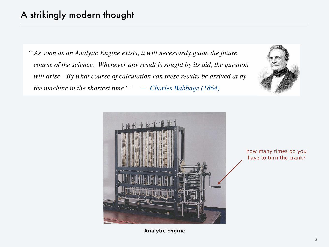
A strikingly modern thought

3

Analytic Engine

“ As soon as an Analytic Engine exists, it will necessarily guide the future course of the science. Whenever any result is sought by its aid, the question will arise—By what course of calculation can these results be arrived at by the machine in the shortest time? ” — Charles Babbage (1864)

how many times do you have to turn the crank?

Brute force

Brute force. For many nontrivial problems, there is a natural brute-force

search algorithm that checks every possible solution.

・Typically takes 2n time or worse for inputs of size n.

・Unacceptable in practice.

4

von Neumann(1953)

Gödel(1956)

Edmonds(1965)

Rabin(1966)

Cobham(1964)

Nash(1955)

Polynomial running time

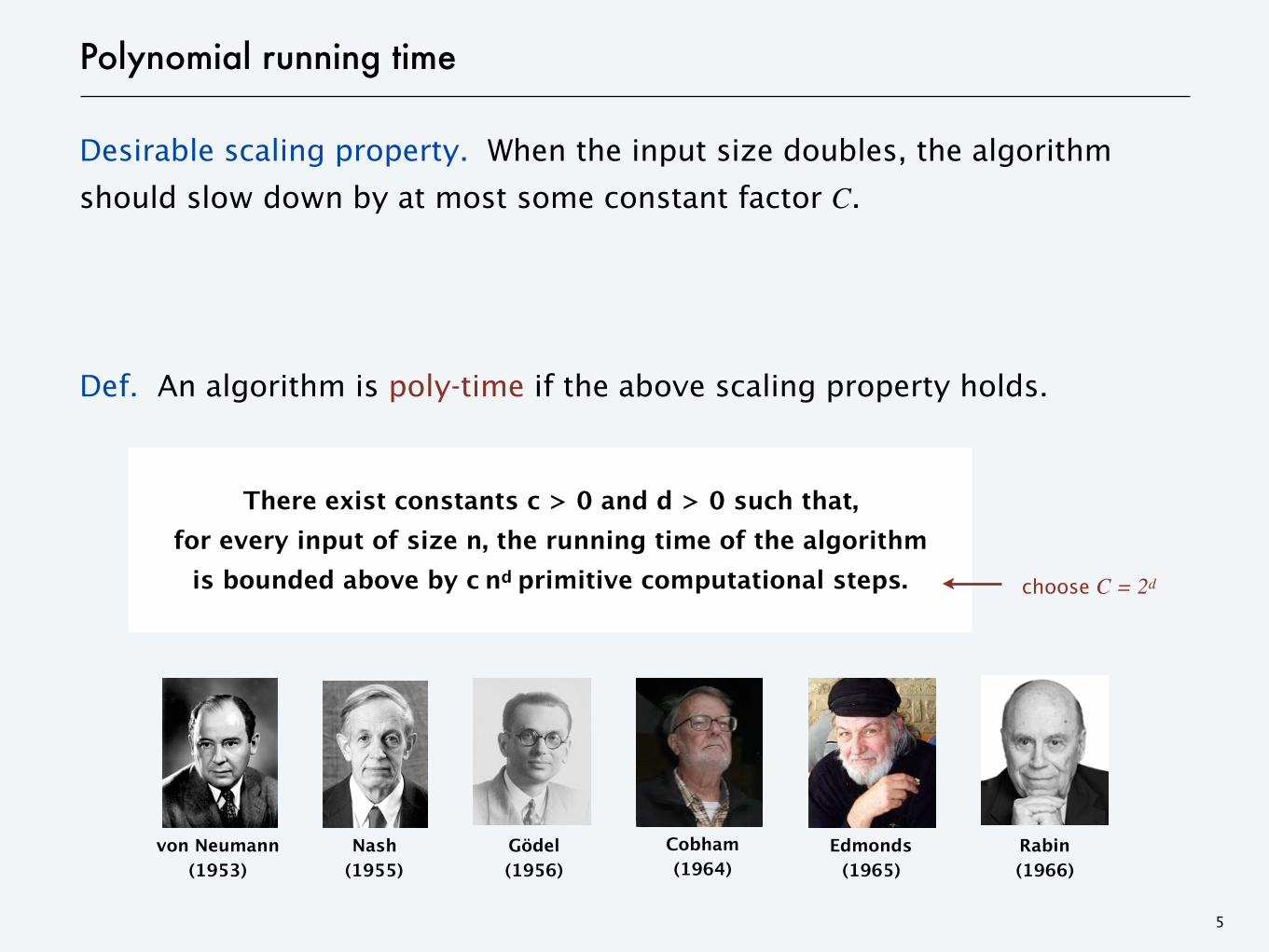
Desirable scaling property. When the input size doubles, the algorithm

should slow down by at most some constant factor C.

Def. An algorithm is poly-time if the above scaling property holds.

5

choose C = 2d

There exist constants c > 0 and d > 0 such that,for every input of size n, the running time of the algorithm

is bounded above by c nd primitive computational steps.

Polynomial running time

We say that an algorithm is efficient if it has a polynomial running time.

Justification. It really works in practice!

・In practice, the poly-time algorithms that people develop have low

constants and low exponents.

・Breaking through the exponential barrier of brute force typically

exposes some crucial structure of the problem.

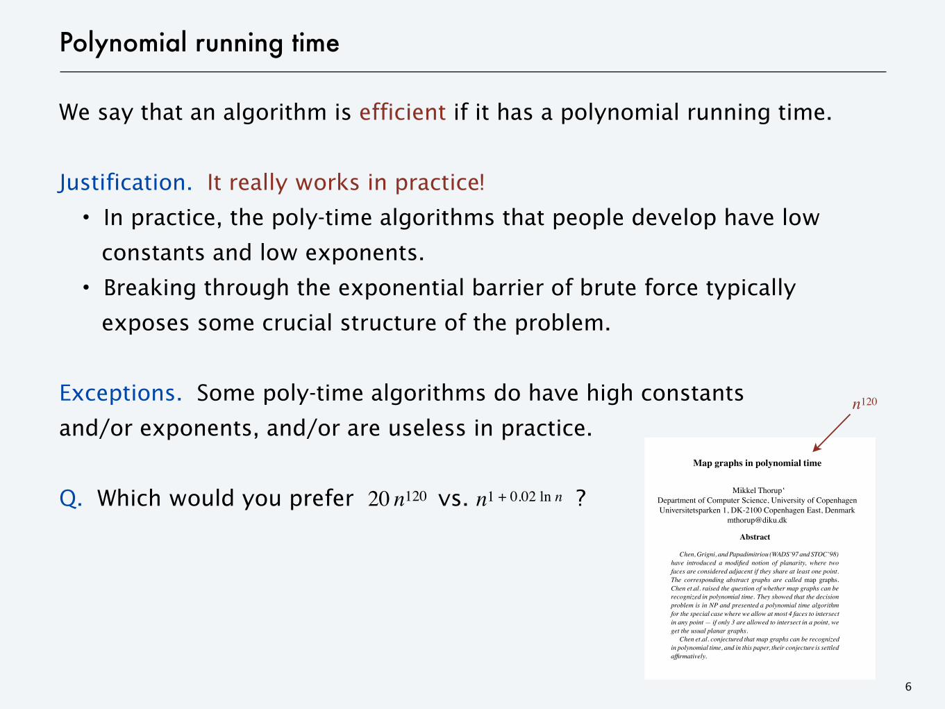
Exceptions. Some poly-time algorithms do have high constantsand/or exponents, and/or are useless in practice.

Q. Which would you prefer 20 n120 vs. n1 + 0.02 ln n ?

6

Map graphs in polynomial time

Mikkel ThorupDepartment of Computer Science, University of CopenhagenUniversitetsparken 1, DK-2100 Copenhagen East, Denmark

mthorup@diku.dk

Abstract

Chen,Grigni, andPapadimitriou (WADS’97 andSTOC’98)have introduced a modified notion of planarity, where twofaces are considered adjacent if they share at least one point.The corresponding abstract graphs are called map graphs.Chen et.al. raised the question of whether map graphs can berecognized in polynomial time. They showed that the decisionproblem is in NP and presented a polynomial time algorithmfor the special case where we allow at most 4 faces to intersectin any point — if only 3 are allowed to intersect in a point, weget the usual planar graphs.

Chen et.al. conjectured that map graphs can be recognizedin polynomial time, and in this paper, their conjecture is settledaffirmatively.

1. Introduction

Recently Chen, Grigni, and Papadimitriou [4, 5] suggestedthe study of a modified notion of planarity. The basic frame-work is the same as that of planar graphs. We are given a set ofnon-overlapping faces in the plane, each being a disc homeo-morphism. By non-overlapping, we mean that two faces mayonly intersect in their boundaries. The plane may or may notbe completely covered by the faces. A traditional planar graphis obtained as follows. The vertices are the faces, and twofaces are neighbors if their intersection contains a non-trivialcurve. Chen et.al. [4, 5] suggested simplifying the definition,by saying that two faces are neighbors if and only if they in-tersect in at least one point. They called the resulting graphs“planar map graphs”. Here we will just call themmap graphs.Note that there are non-planar map graphs, for as illustratedin Figure 1, map graphs can contain arbitrarily large cliques.We shall refer to the first type of clique as a flower with thepetals intersecting in a center. The second is a hamantashbased on three distinct corner points. Each of the three pairsof corner points is connected by a side of parallel faces. In

Most of this work was done while the author visited MIT.Chen et.al. called flowers for pizzas, but “flower” seems more natural.

Figure 1. Large cliques in maps

addition, the hamantach may have at most two triangle facestouching all three corners. In [5] there is a classification ofall the different types of large cliques in maps. Chen et.al. [5]showed that recognizing map graphs is in NP, hence that therecognition can be done in singly exponential time. However,they conjectured that, in fact, map graphs can be recognized inpolynomial time. They supported their conjecture by showingthat if we allow at most 4 faces to meet in any single point, theresultingmap graphs can be recognized in polynomial time. Inthis paper, we settle the general conjecture, showing that givena graph, we can decide in polynomial time if it is a map graph.The algorithm can easily be modified to draw a correspondingmap if it exists.

Map coloring It should be noted that coloring of map graphsdates back to Ore and Plummer in 1969 [8], that is, theywantedto color the faces so that any two intersecting facesgot differentcolors. For an account of colorful history, the reader is referredto [7, 2.5]. In particular, the history provides an answer to aproblem of Chen et.al. [5]: if at most 4 facesmeet in any singlepoint, canwe color themapwith 6 colors? It is straightforwardto see that the resulting graphs are 1-planar, meaning that theycan be drawn in the plane such that each edge is crossed by atmost one other edge. Already in 1965, Ringel [9] conjecturedthat all 1-planar graphs can be colored with 6 colors, and thisconjecture was settled in 1984 by Borodin [2], so the answerto Chen et.al.’s problem is: yes.

Map metrics The shortest path metrics of map graphs arecommonly used in prizing systems, where you pay for cross-

Map graphs in polynomial time

Mikkel ThorupDepartment of Computer Science, University of CopenhagenUniversitetsparken 1, DK-2100 Copenhagen East, Denmark

mthorup@diku.dk

Abstract

Chen,Grigni, andPapadimitriou (WADS’97 andSTOC’98)have introduced a modified notion of planarity, where twofaces are considered adjacent if they share at least one point.The corresponding abstract graphs are called map graphs.Chen et.al. raised the question of whether map graphs can berecognized in polynomial time. They showed that the decisionproblem is in NP and presented a polynomial time algorithmfor the special case where we allow at most 4 faces to intersectin any point — if only 3 are allowed to intersect in a point, weget the usual planar graphs.

Chen et.al. conjectured that map graphs can be recognizedin polynomial time, and in this paper, their conjecture is settledaffirmatively.

1. Introduction

Recently Chen, Grigni, and Papadimitriou [4, 5] suggestedthe study of a modified notion of planarity. The basic frame-work is the same as that of planar graphs. We are given a set ofnon-overlapping faces in the plane, each being a disc homeo-morphism. By non-overlapping, we mean that two faces mayonly intersect in their boundaries. The plane may or may notbe completely covered by the faces. A traditional planar graphis obtained as follows. The vertices are the faces, and twofaces are neighbors if their intersection contains a non-trivialcurve. Chen et.al. [4, 5] suggested simplifying the definition,by saying that two faces are neighbors if and only if they in-tersect in at least one point. They called the resulting graphs“planar map graphs”. Here we will just call themmap graphs.Note that there are non-planar map graphs, for as illustratedin Figure 1, map graphs can contain arbitrarily large cliques.We shall refer to the first type of clique as a flower with thepetals intersecting in a center. The second is a hamantashbased on three distinct corner points. Each of the three pairsof corner points is connected by a side of parallel faces. In

Most of this work was done while the author visited MIT.Chen et.al. called flowers for pizzas, but “flower” seems more natural.

Figure 1. Large cliques in maps

addition, the hamantach may have at most two triangle facestouching all three corners. In [5] there is a classification ofall the different types of large cliques in maps. Chen et.al. [5]showed that recognizing map graphs is in NP, hence that therecognition can be done in singly exponential time. However,they conjectured that, in fact, map graphs can be recognized inpolynomial time. They supported their conjecture by showingthat if we allow at most 4 faces to meet in any single point, theresultingmap graphs can be recognized in polynomial time. Inthis paper, we settle the general conjecture, showing that givena graph, we can decide in polynomial time if it is a map graph.The algorithm can easily be modified to draw a correspondingmap if it exists.

Map coloring It should be noted that coloring of map graphsdates back to Ore and Plummer in 1969 [8], that is, theywantedto color the faces so that any two intersecting facesgot differentcolors. For an account of colorful history, the reader is referredto [7, 2.5]. In particular, the history provides an answer to aproblem of Chen et.al. [5]: if at most 4 facesmeet in any singlepoint, canwe color themapwith 6 colors? It is straightforwardto see that the resulting graphs are 1-planar, meaning that theycan be drawn in the plane such that each edge is crossed by atmost one other edge. Already in 1965, Ringel [9] conjecturedthat all 1-planar graphs can be colored with 6 colors, and thisconjecture was settled in 1984 by Borodin [2], so the answerto Chen et.al.’s problem is: yes.

Map metrics The shortest path metrics of map graphs arecommonly used in prizing systems, where you pay for cross-

n120

Worst-case analysis

Worst case. Running time guarantee for any input of size n.

・Generally captures efficiency in practice.

・Draconian view, but hard to find effective alternative.

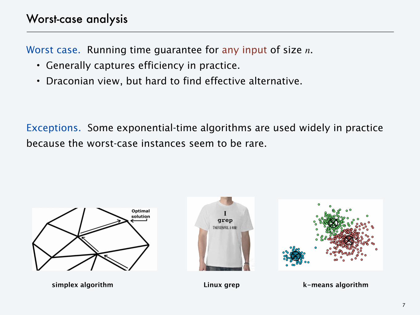
Exceptions. Some exponential-time algorithms are used widely in practice

because the worst-case instances seem to be rare.

7

simplex algorithm Linux grep k-means algorithm

Types of analyses

Worst case. Running time guarantee for any input of size n. Ex. Heapsort requires at most 2 n log2 n compares to sort n elements.

Probabilistic. Expected running time of a randomized algorithm. Ex. The expected number of compares to quicksort n elements is ~ 2n ln n.

Amortized. Worst-case running time for any sequence of n operations. Ex. Starting from an empty stack, any sequence of n push and pop

operations takes O(n) primitive computational steps using a resizing array.

Average-case. Expected running time for a random input of size n. Ex. The expected number of character compares performed by 3-way radix quicksort on n uniformly random strings is ~ 2n ln n.

Also. Smoothed analysis, competitive analysis, ...

8

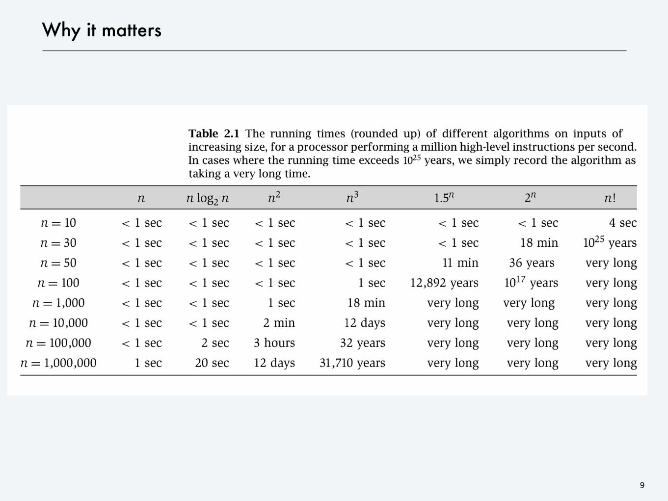
Why it matters

9

2. ALGORITHM ANALYSIS

‣ computational tractability

‣ asymptotic order of growth

‣ survey of common running times

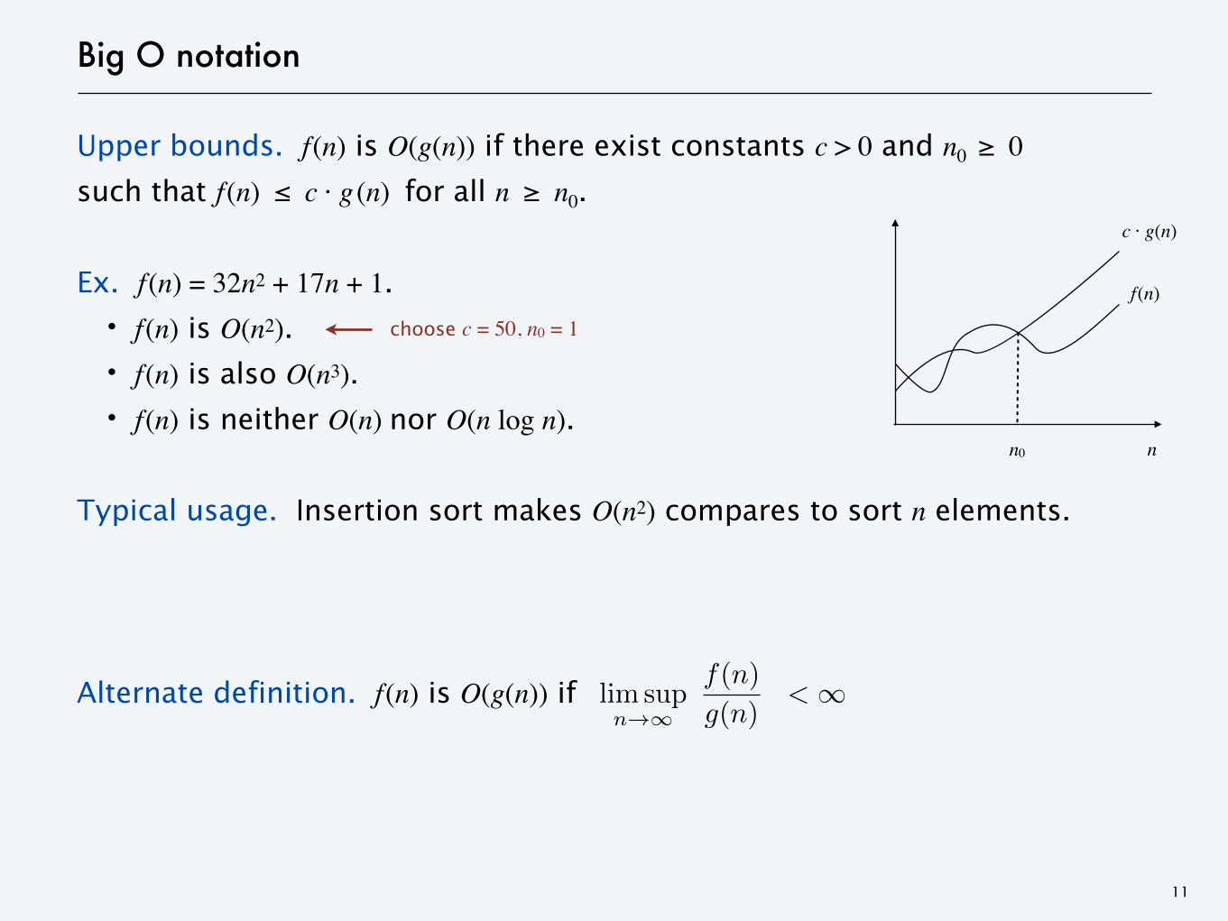
Big O notation

Upper bounds. f(n) is O(g(n)) if there exist constants c > 0 and n0 ≥ 0 such that f(n) ≤ c · g (n) for all n ≥ n0.

Ex. f(n) = 32n2 + 17n + 1.

・f(n) is O(n2).

・f(n) is also O(n3).

・f(n) is neither O(n) nor O(n log n).

Typical usage. Insertion sort makes O(n2) compares to sort n elements.

Alternate definition. f(n) is O(g(n)) if

11

choose c = 50, n0 = 1

c · g(n)

nn0

f(n)

lim supn��

f(n)

g(n)< �

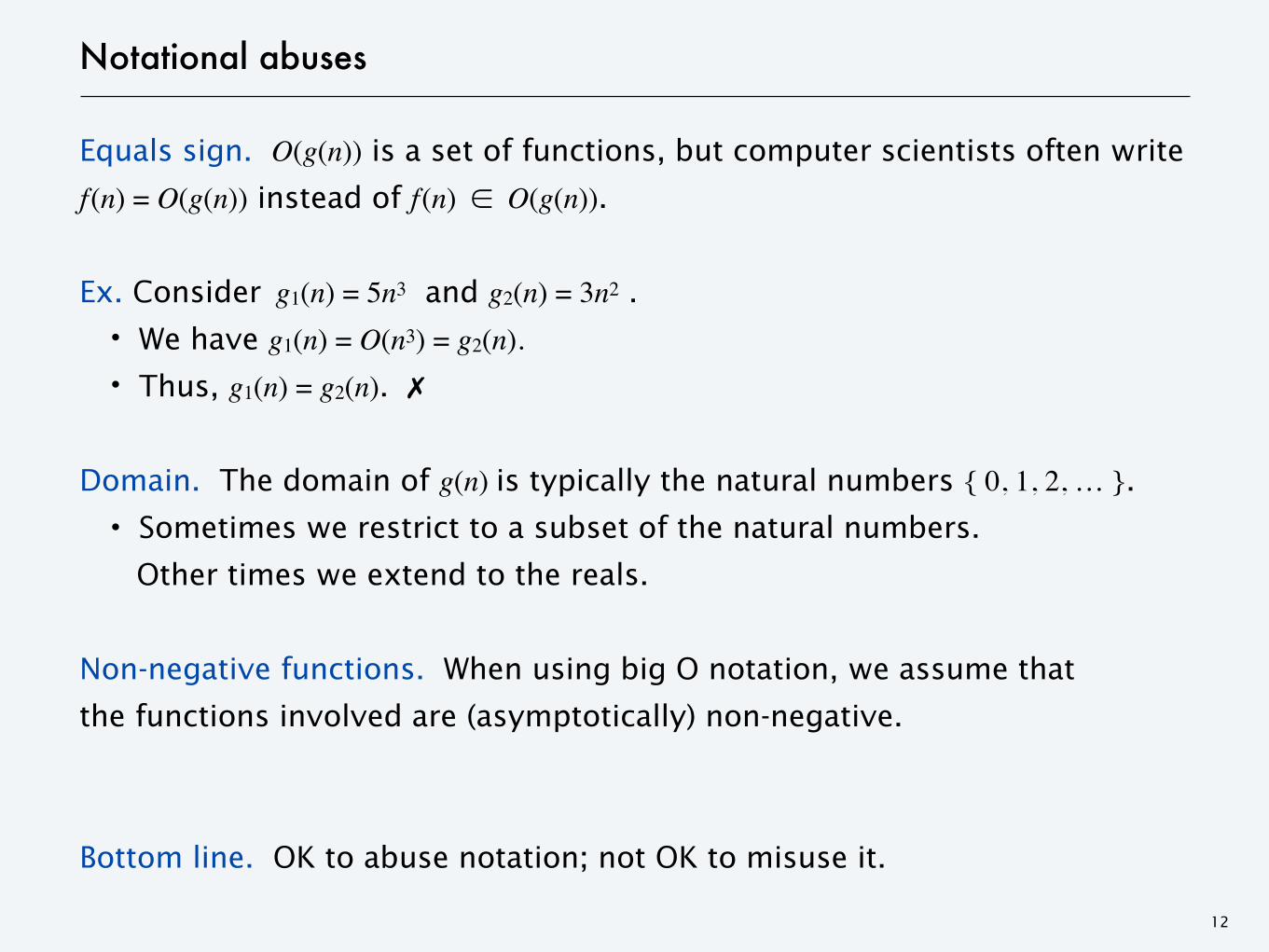
Notational abuses

Equals sign. O(g(n)) is a set of functions, but computer scientists often write f(n) = O(g(n)) instead of f(n) ∈ O(g(n)). Ex. Consider g1(n) = 5n3 and g2(n) = 3n2 .

・We have g1(n) = O(n3) = g2(n).

・Thus, g1(n) = g2(n). ✗

Domain. The domain of g(n) is typically the natural numbers { 0, 1, 2, … }.

・Sometimes we restrict to a subset of the natural numbers.Other times we extend to the reals.

Non-negative functions. When using big O notation, we assume thatthe functions involved are (asymptotically) non-negative.

Bottom line. OK to abuse notation; not OK to misuse it.

12

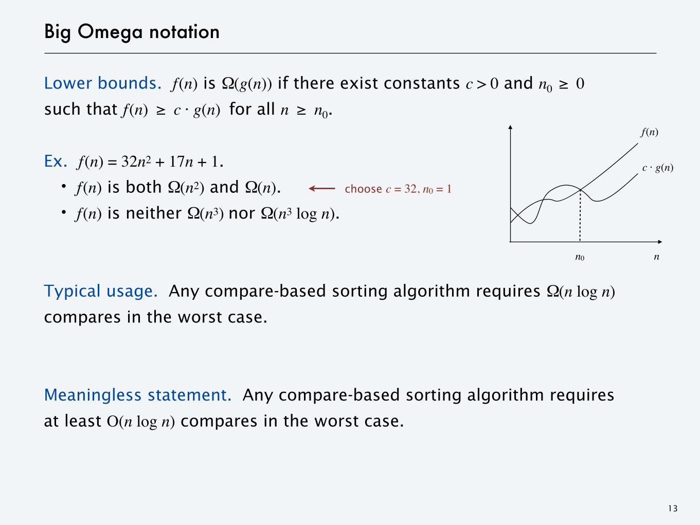
Big Omega notation

Lower bounds. f(n) is Ω(g(n)) if there exist constants c > 0 and n0 ≥ 0 such that f(n) ≥ c · g(n) for all n ≥ n0.

Ex. f(n) = 32n2 + 17n + 1.

・f(n) is both Ω(n2) and Ω(n).

・f(n) is neither Ω(n3) nor Ω(n3 log n). Typical usage. Any compare-based sorting algorithm requires Ω(n log n) compares in the worst case.

Meaningless statement. Any compare-based sorting algorithm requires at least O(n log n) compares in the worst case.

13

choose c = 32, n0 = 1

f(n)

nn0

c · g(n)

Big Theta notation

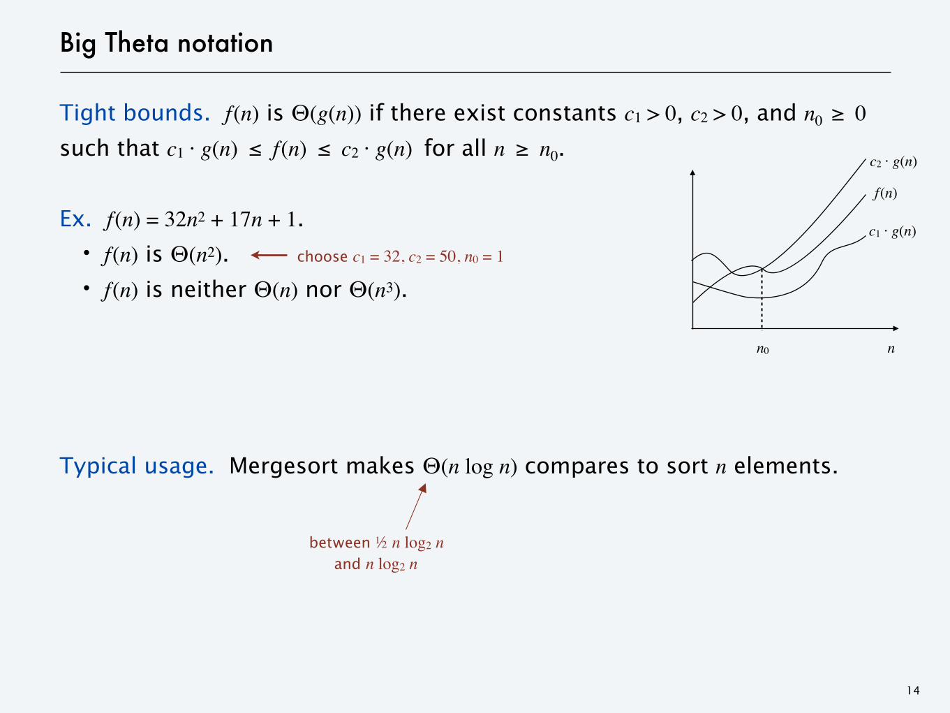
Tight bounds. f(n) is Θ(g(n)) if there exist constants c1 > 0, c2 > 0, and n0 ≥ 0 such that c1 · g(n) ≤ f(n) ≤ c2 · g(n) for all n ≥ n0.

Ex. f(n) = 32n2 + 17n + 1.

・f(n) is Θ(n2).

・f(n) is neither Θ(n) nor Θ(n3). Typical usage. Mergesort makes Θ(n log n) compares to sort n elements.

14

choose c1 = 32, c2 = 50, n0 = 1

f(n)

nn0

c1 · g(n)

c2 · g(n)

between ½ n log2 nand n log2 n

Useful facts

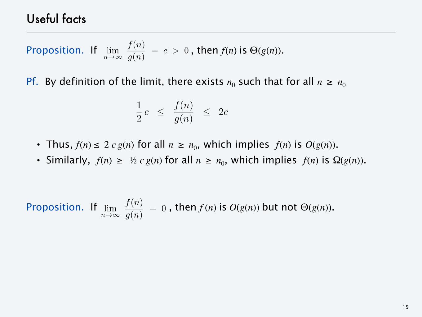
Proposition. If , then f(n) is Θ(g(n)). Pf. By definition of the limit, there exists n0 such that for all n ≥ n0

・Thus, f(n) ≤ 2 c g(n) for all n ≥ n0, which implies f(n) is O(g(n)).

・Similarly, f(n) ≥ ½ c g(n) for all n ≥ n0, which implies f(n) is Ω(g(n)). Proposition. If , then f (n) is O(g(n)) but not Θ(g(n)).

15

limn��

f(n)

g(n)= c > 0

limn��

f(n)

g(n)= 0

1

2c � f(n)

g(n)� 2c

Asymptotic bounds for some common functions

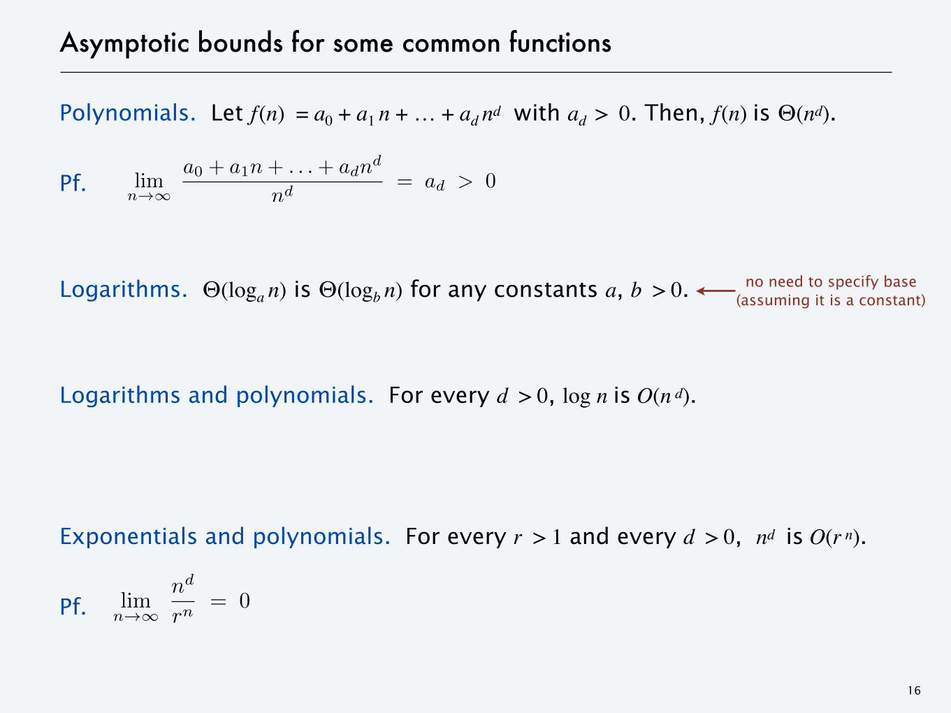
Polynomials. Let f(n) = a0 + a1 n + … + ad nd with ad > 0. Then, f(n) is Θ(nd). Pf.

Logarithms. Θ(loga n) is Θ(logb n) for any constants a, b > 0.

Logarithms and polynomials. For every d > 0, log n is O(n d). Exponentials and polynomials. For every r > 1 and every d > 0, nd is O(r n). Pf.

16

no need to specify base(assuming it is a constant)

limn��

a0 + a1n + . . . + adnd

nd= ad > 0

limn��

nd

rn= 0

Big O notation with multiple variables

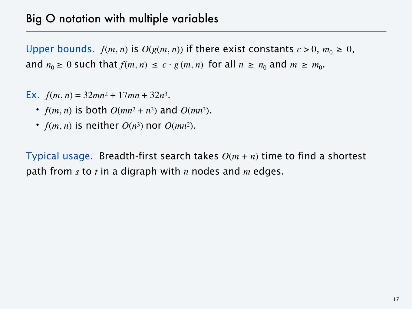
Upper bounds. f(m, n) is O(g(m, n)) if there exist constants c > 0, m0 ≥ 0,and n0 ≥ 0 such that f(m, n) ≤ c · g (m, n) for all n ≥ n0 and m ≥ m0.

Ex. f(m, n) = 32mn2 + 17mn + 32n3.

・f(m, n) is both O(mn2 + n3) and O(mn3).

・f(m, n) is neither O(n3) nor O(mn2).

Typical usage. Breadth-first search takes O(m + n) time to find a shortest

path from s to t in a digraph with n nodes and m edges.

17

2. ALGORITHM ANALYSIS

‣ computational tractability

‣ asymptotic order of growth

‣ survey of common running times

Linear time: O(n)

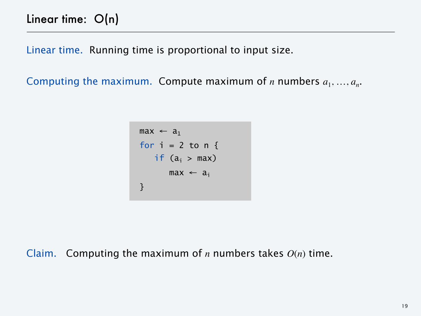
Linear time. Running time is proportional to input size.

Computing the maximum. Compute maximum of n numbers a1, …, an.

Claim. Computing the maximum of n numbers takes O(n) time.

19

max ← a1 for i = 2 to n { if (ai > max)

max ← ai }

Linear time: O(n)

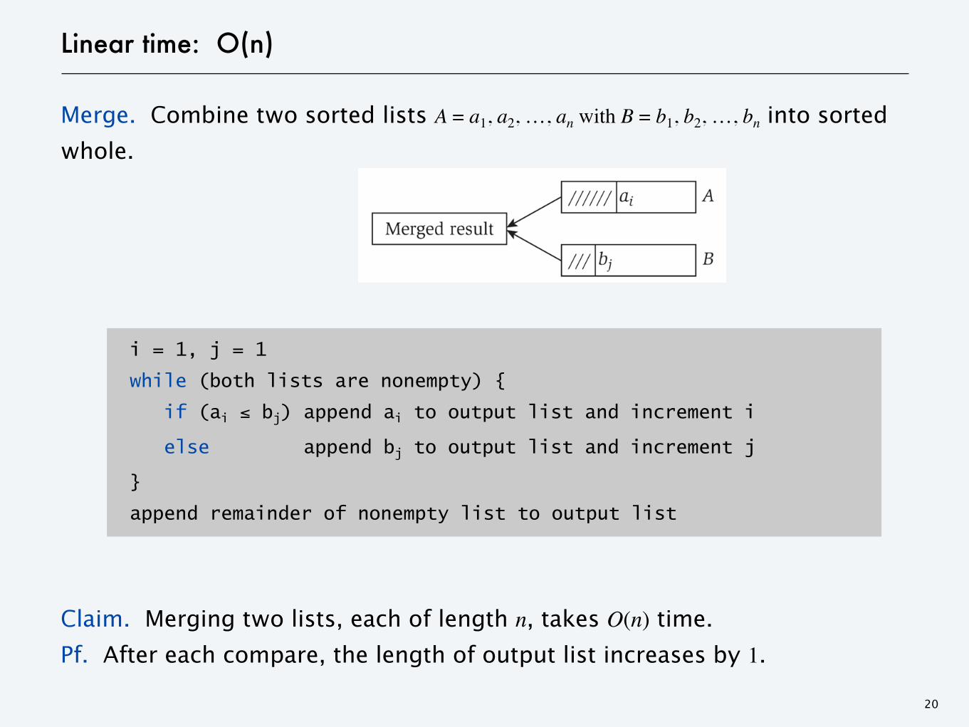
Merge. Combine two sorted lists A = a1, a2, …, an with B = b1, b2, …, bn into sorted

whole.

Claim. Merging two lists, each of length n, takes O(n) time.

Pf. After each compare, the length of output list increases by 1.

20

i = 1, j = 1

while (both lists are nonempty) {

if (ai ≤ bj) append ai to output list and increment i

else(ai ≤ bj)append bj to output list and increment j

}

append remainder of nonempty list to output list

Linearithmic time: O(n log n)

O(n log n) time. Arises in divide-and-conquer algorithms.

Sorting. Mergesort and heapsort are sorting algorithms that performO(n log n) compares.

Largest empty interval. Given n time stamps x1, …, xn on which copies of a

file arrive at a server, what is largest interval when no copies of file arrive?

O(n log n) solution. Sort the time stamps. Scan the sorted list in order,

identifying the maximum gap between successive time-stamps.

21

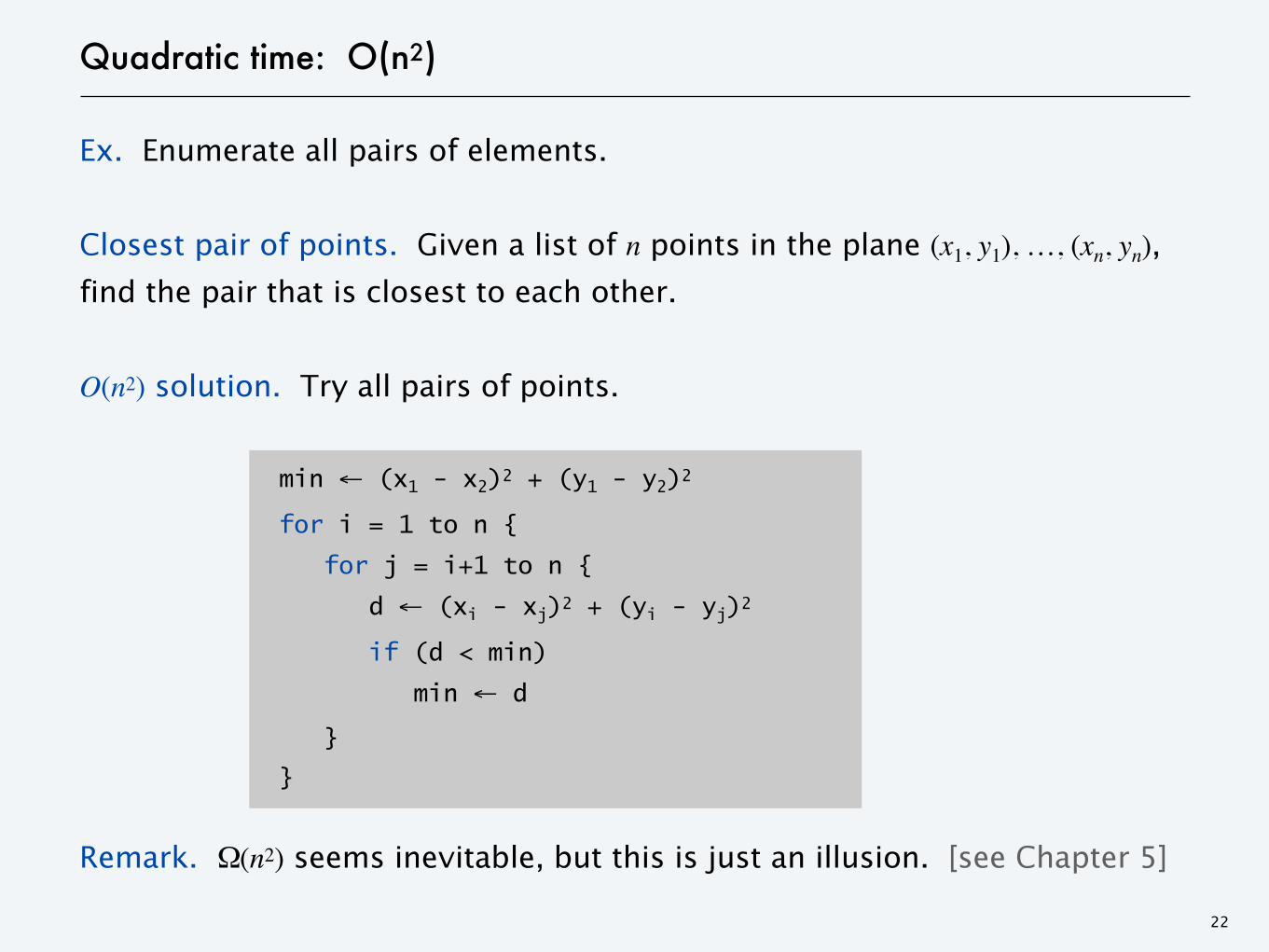
Quadratic time: O(n2)

Ex. Enumerate all pairs of elements.

Closest pair of points. Given a list of n points in the plane (x1, y1), …, (xn, yn), find the pair that is closest to each other.

O(n2) solution. Try all pairs of points.

Remark. Ω(n2) seems inevitable, but this is just an illusion. [see Chapter 5]

22

min ← (x1 - x2)2 + (y1 - y2)2

for i = 1 to n {

for j = i+1 to n {

d ← (xi - xj)2 + (yi - yj)2

if (d < min)

min ← d

}

}

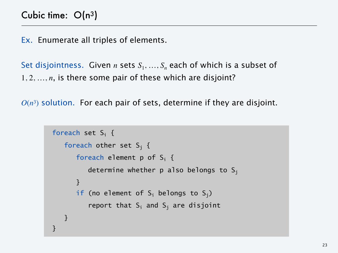
Cubic time: O(n3)

Ex. Enumerate all triples of elements.

Set disjointness. Given n sets S1, …, Sn each of which is a subset of 1, 2, …, n, is there some pair of these which are disjoint?

O(n3) solution. For each pair of sets, determine if they are disjoint.

23

foreach set Si {

foreach other set Sj {

foreach element p of Si {

determine whether p also belongs to Sj

}

if (no element of Si belongs to Sj)

report that Si and Sj are disjoint

}

}

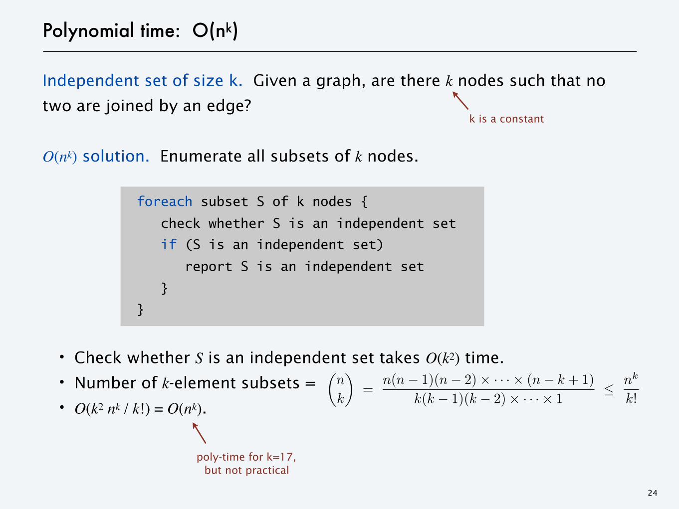
Polynomial time: O(nk)

Independent set of size k. Given a graph, are there k nodes such that no

two are joined by an edge?

O(nk) solution. Enumerate all subsets of k nodes.

・Check whether S is an independent set takes O(k2) time.

・Number of k-element subsets =

・O(k2 nk / k!) = O(nk).

24

foreach subset S of k nodes {

check whether S is an independent set

if (S is an independent set)

report S is an independent set

}

}

poly-time for k=17,but not practical

k is a constant

�n

k

�=

n(n � 1)(n � 2) � · · · � (n � k + 1)

k(k � 1)(k � 2) � · · · � 1� nk

k!

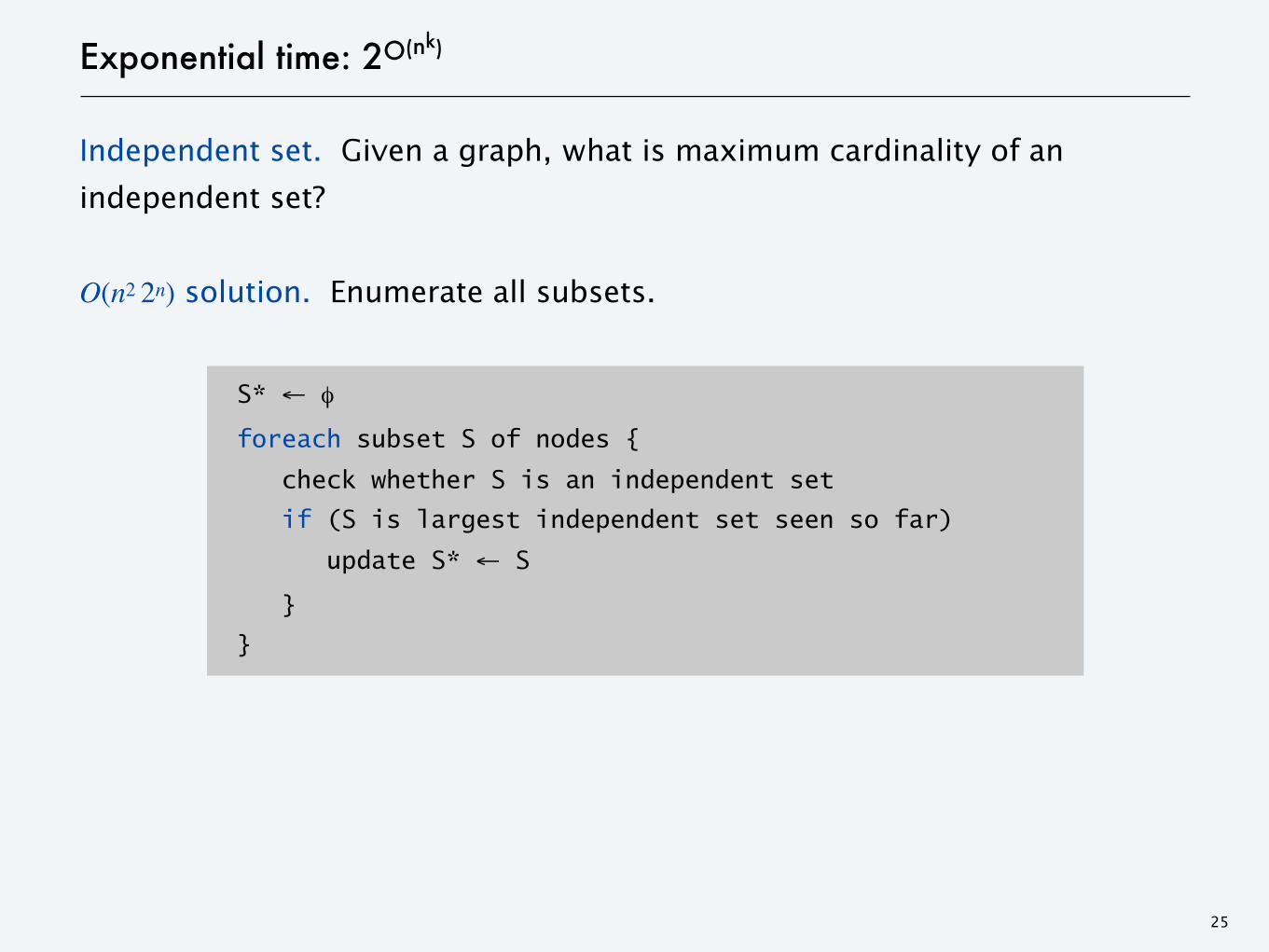
Exponential time: 2O(nk)

Independent set. Given a graph, what is maximum cardinality of an

independent set?

O(n2 2n) solution. Enumerate all subsets.

25

S* ← φ

foreach subset S of nodes {

check whether S is an independent set

if (S is largest independent set seen so far)

update S* ← S

}

}

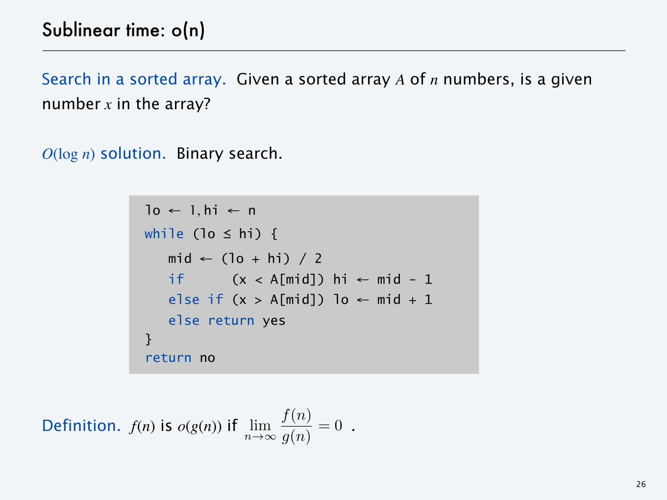
Sublinear time: o(n)

Search in a sorted array. Given a sorted array A of n numbers, is a given

number x in the array?

O(log n) solution. Binary search.

Definition. f(n) is o(g(n)) if .

26

lo ← 1, hi ← n

while (lo ≤ hi) { mid ← (lo + hi) / 2

if (x < A[mid]) hi ← mid - 1 else if (x > A[mid]) lo ← mid + 1

else return yes } return no

limn��

f(n)

g(n)= 0