2-10 Redes RLC

Ciclo I-2014 UES-FIA-EIE-AEL115

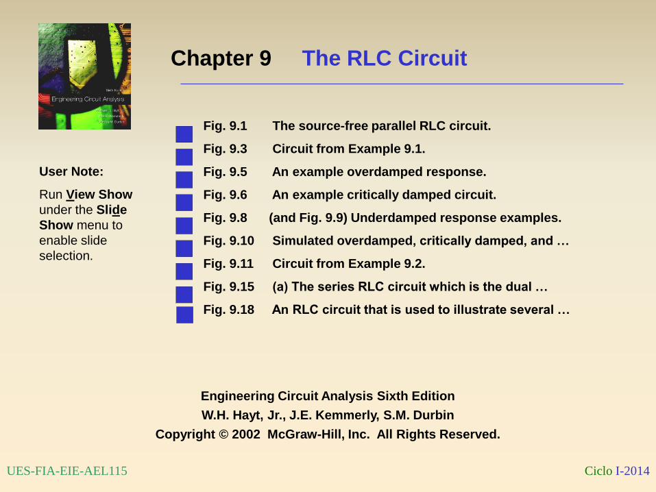
Chapter 9 The RLC Circuit

Engineering Circuit Analysis Sixth Edition

W.H. Hayt, Jr., J.E. Kemmerly, S.M. Durbin

Copyright © 2002 McGraw-Hill, Inc. All Rights Reserved.

User Note:

Run View Show

under the Slide

Show menu to

enable slide

selection.

Fig. 9.1 The source-free parallel RLC circuit.

Fig. 9.3 Circuit from Example 9.1.

Fig. 9.5 An example overdamped response.

Fig. 9.6 An example critically damped circuit.

Fig. 9.8 (and Fig. 9.9) Underdamped response examples.

Fig. 9.10 Simulated overdamped, critically damped, and …

Fig. 9.11 Circuit from Example 9.2.

Fig. 9.15 (a) The series RLC circuit which is the dual …

Fig. 9.18 An RLC circuit that is used to illustrate several …

http://www.mhhe.com/hayt6e


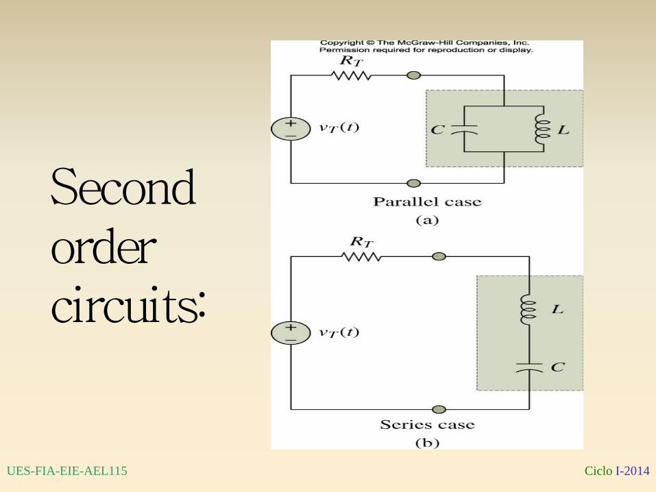
Figure 5.38 Second

order circuits:


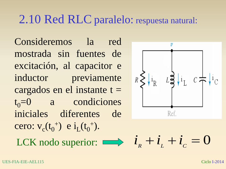
Consideremos la red

mostrada sin fuentes de

excitación, al capacitor e

inductor previamente

cargados en el instante t =

t0=0 a condiciones

iniciales diferentes de

cero: vc(t0+) e iL(t0

+).

LCK nodo superior: 0CLRiii

2.10 Red RLC paralelo: respuesta natural:


0)(1

0

0

dt

dvCtivdt

LR

v t

tL

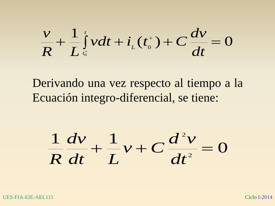
Derivando una vez respecto al tiempo a la

Ecuación integro-diferencial, se tiene:

011

2

2

dt

vdCv

Ldt

dv

R


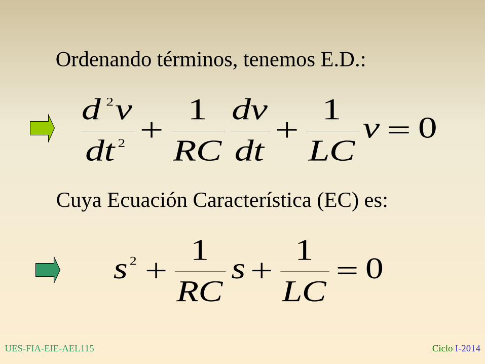
Ordenando términos, tenemos E.D.:

011

2

2

vLCdt

dv

RCdt

vd

Cuya Ecuación Característica (EC) es:

0112

LCs

RCs


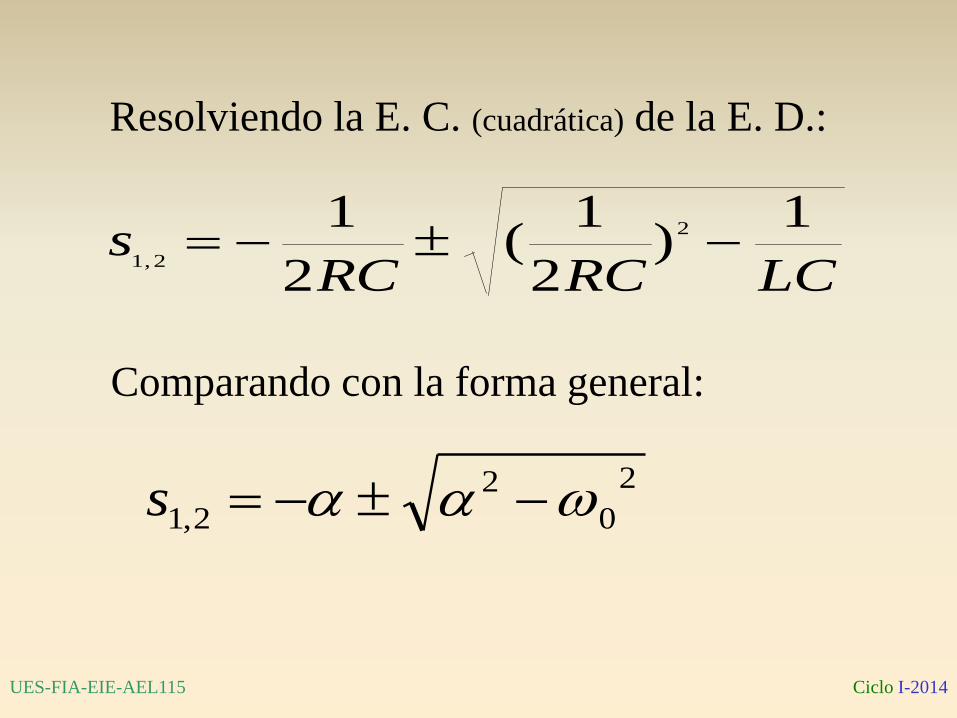
Resolviendo la E. C. (cuadrática) de la E. D.:

Comparando con la forma general:

LCRCRCs

1)

2

1(

2

1 2

2,1

2

0

2

2,1 s


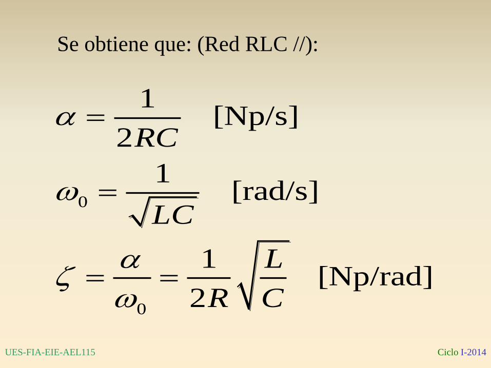
Se obtiene que: (Red RLC //):

0

0

1 [Np/s]

2

1 [rad/s]

1 [Np/rad]

2

RC

LC

L

R C


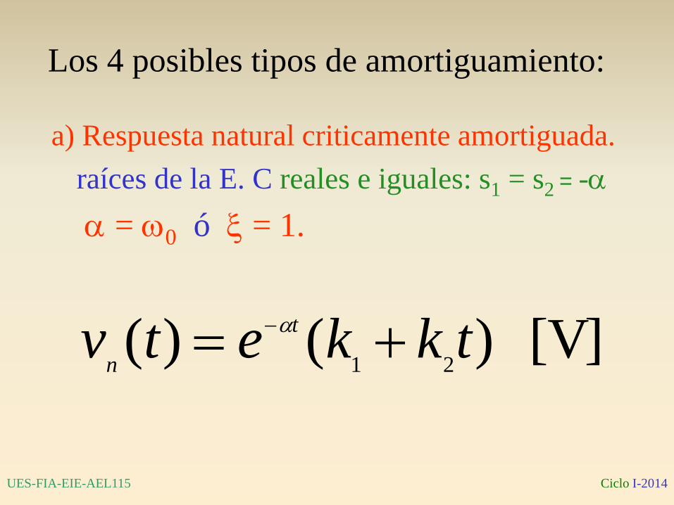
[V] )()(21tkketv t

n

a) Respuesta natural criticamente amortiguada.

raíces de la E. C reales e iguales: s1 = s2 = -

= 0 ó = 1.

Los 4 posibles tipos de amortiguamiento:


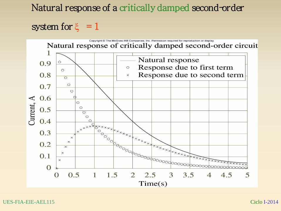
Figure 5.46

Natural response of a critically damped second-order

system for = 1


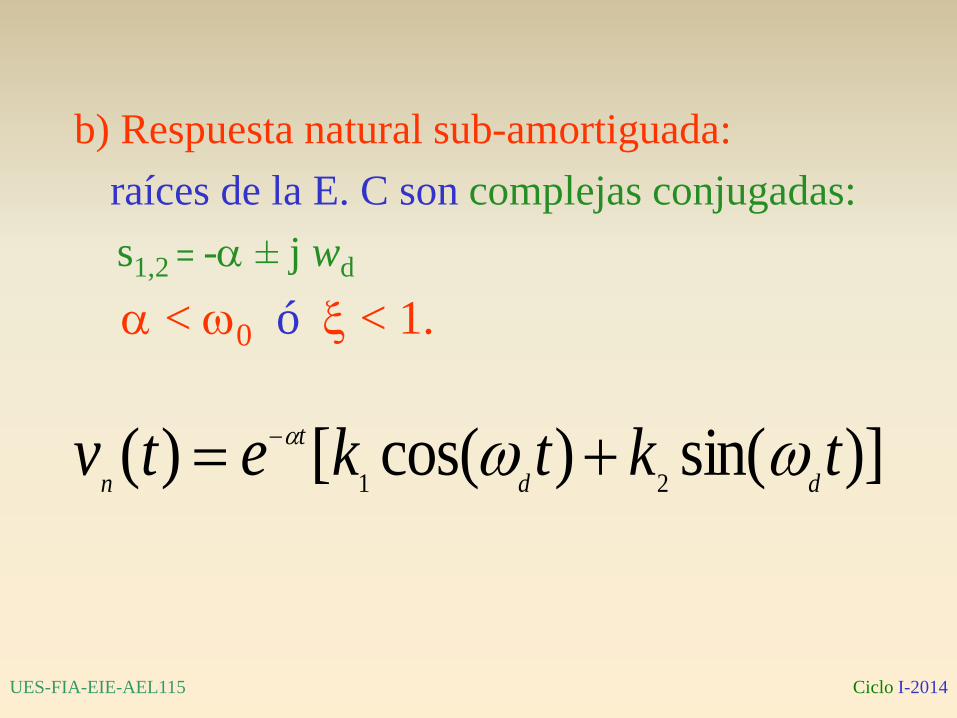
b) Respuesta natural sub-amortiguada:

raíces de la E. C son complejas conjugadas:

s1,2 = - ± j wd

< 0 ó < 1.

)]sin()cos([)(21

tktketvdd

t

n


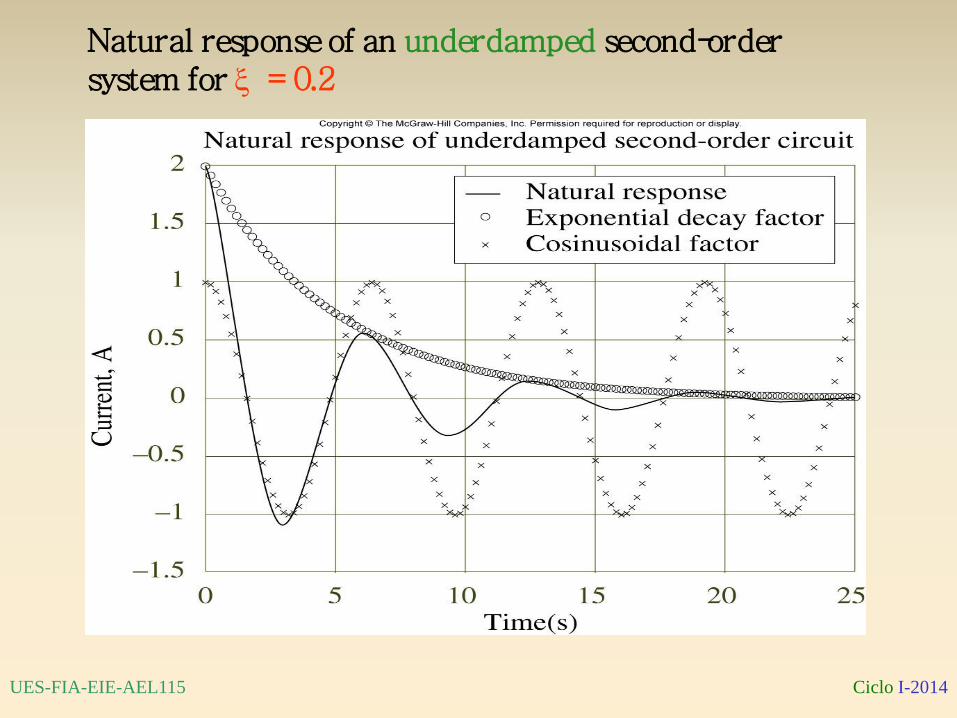
Figure 5.47

Natural response of an underdamped second-order system for = 0.2


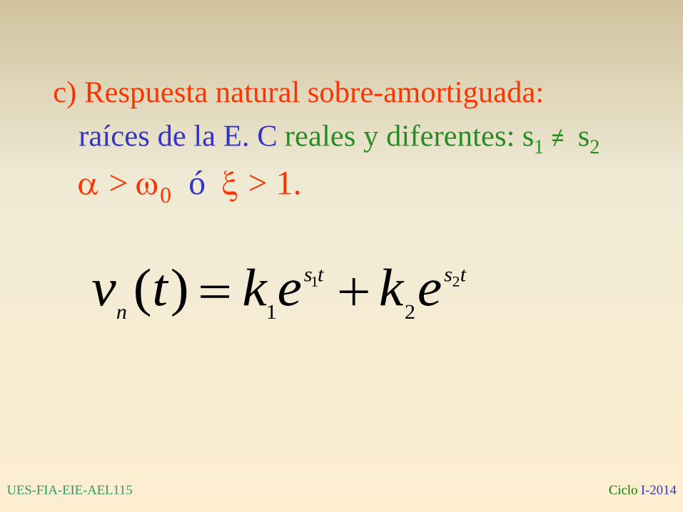
c) Respuesta natural sobre-amortiguada:

raíces de la E. C reales y diferentes: s1 ≠ s2

> 0 ó > 1.

tsts

nekektv 21

21)(


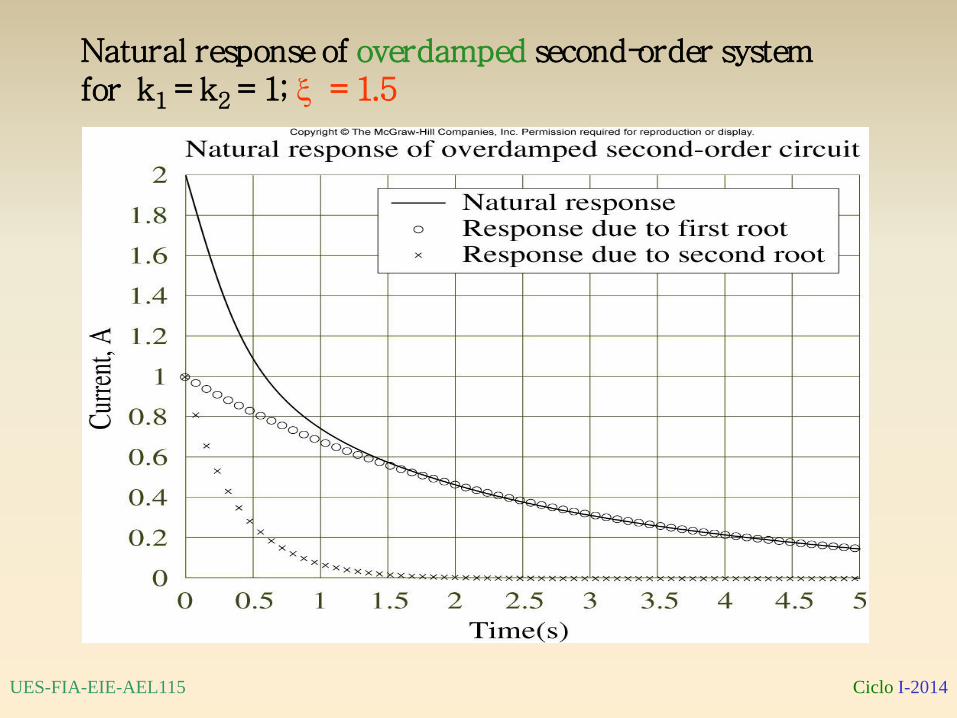
Figure 5.45

Natural response of overdamped second-order system for k1 = k2 = 1; = 1.5


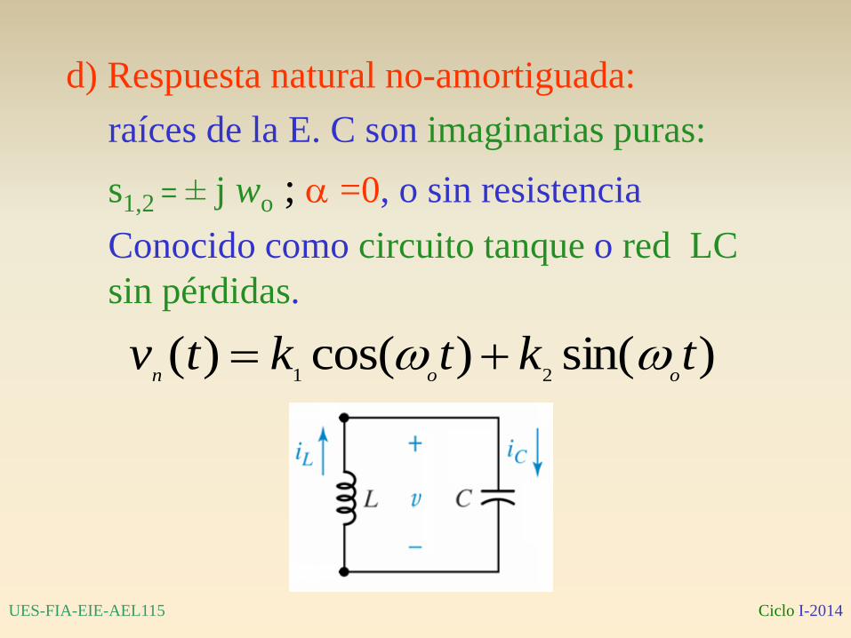
d) Respuesta natural no-amortiguada:

raíces de la E. C son imaginarias puras:

s1,2 = ± j wo ; =0, o sin resistencia

Conocido como circuito tanque o red LC

sin pérdidas.

)sin()cos()(21

tktktvoon


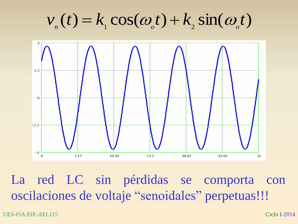
)sin()cos()(21

tktktvoon

La red LC sin pérdidas se comporta con

oscilaciones de voltaje “senoidales” perpetuas!!!


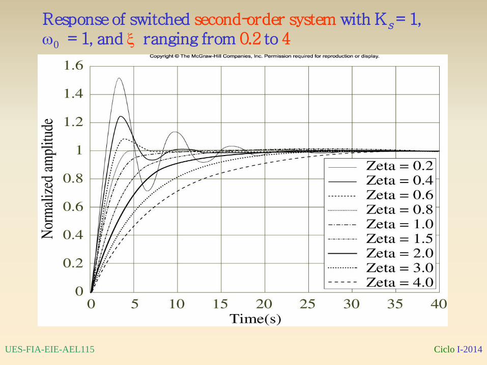
Figure 5.42

Response of switched second-order system with Ks = 1, 0 = 1, and ranging from 0.2 to 4


Conclusiones:

• El tipo de amortiguamiento depende de los

valores de R, L y C lo cual puede resultar en

cualquiera de los 4 casos posibles descritos.

• Las constantes k1 y k2 de la respuesta natural

se determinan evaluando la ec. de la solución

particular en el instante t = t0+: vn(t0+) y

dvn/dt en t0+ y comparando con las

condiciones iniciales o de frontera

determinadas en la red que están sujetas a la

carga inicial en C y L: vc(t0+) e iL(t0

+).


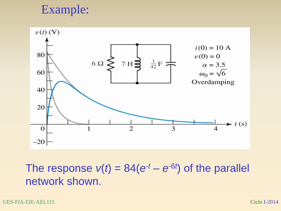
Fig. 9.5 An example

overdamped response.

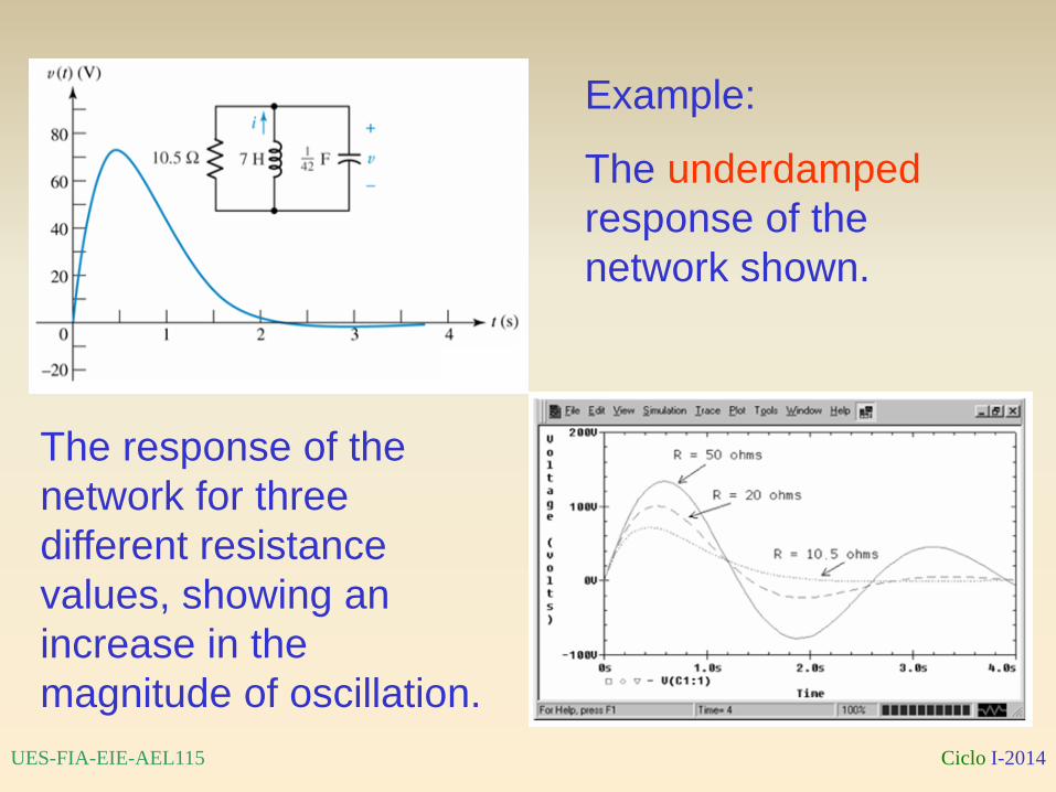
Example:

The response v(t) = 84(e-t – e-6t) of the parallel

network shown.


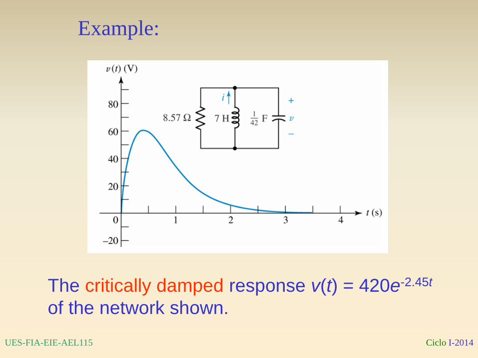
Fig. 9.6 An example critically

damped circuit.

Example:

The critically damped response v(t) = 420e-2.45t

of the network shown.


Fig. 9.8, 9.9 Underdamped

response examples.

Example:

The underdamped

response of the

network shown.

The response of the

network for three

different resistance

values, showing an

increase in the

magnitude of oscillation.


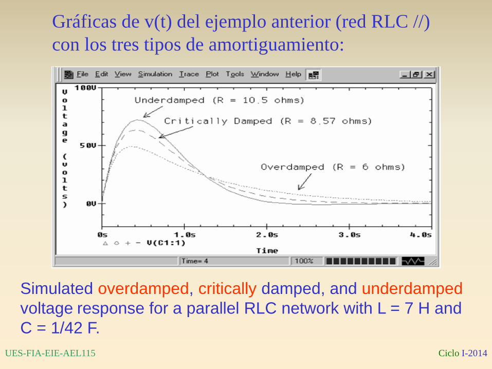
Fig. 9.10 Simulated

overdamped, critically

damped, and underdamped

voltage response for the

example network.

Gráficas de v(t) del ejemplo anterior (red RLC //)

con los tres tipos de amortiguamiento:

Simulated overdamped, critically damped, and underdamped

voltage response for a parallel RLC network with L = 7 H and

C = 1/42 F.


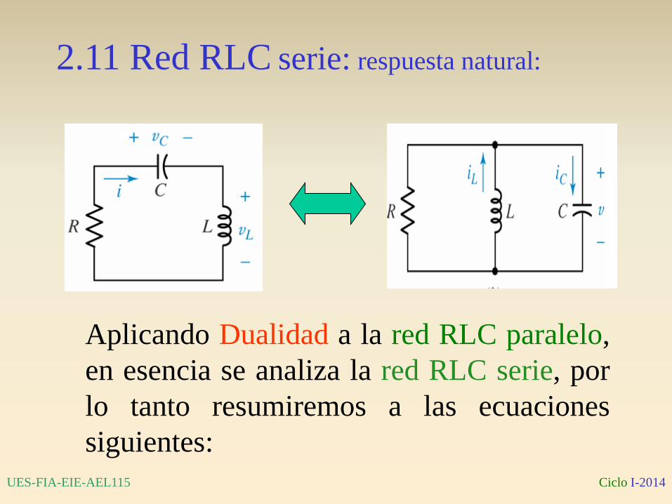
Fig. 9.15 (a) The series RLC

circuit which is the dual of

(b) a parallel RLC circuit.

2.11 Red RLC serie: respuesta natural:

Aplicando Dualidad a la red RLC paralelo,

en esencia se analiza la red RLC serie, por

lo tanto resumiremos a las ecuaciones

siguientes:


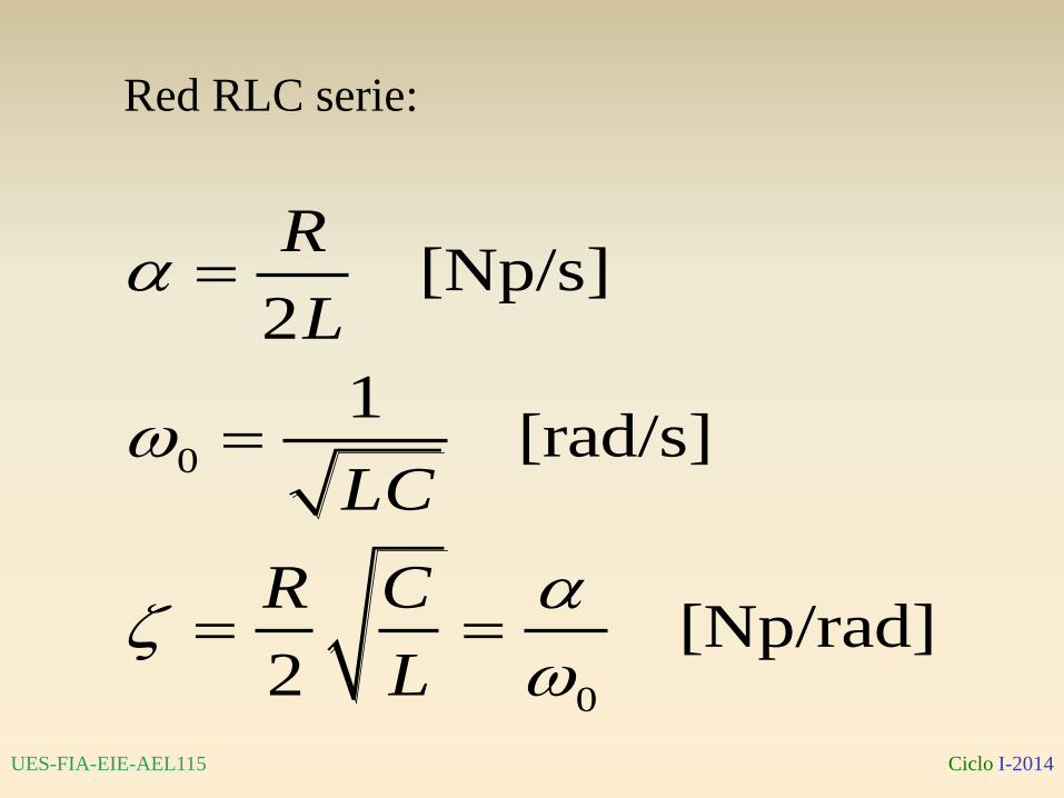
Red RLC serie:

0

0

[Np/s]2

1 [rad/s]

[Np/rad]2

R

L

LC

R C

L


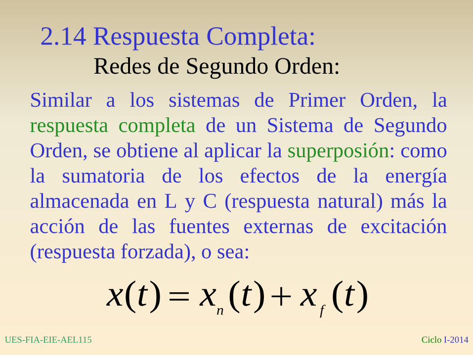
2.14 Respuesta Completa: Redes de Segundo Orden:

Similar a los sistemas de Primer Orden, la

respuesta completa de un Sistema de Segundo

Orden, se obtiene al aplicar la superposión: como

la sumatoria de los efectos de la energía

almacenada en L y C (respuesta natural) más la

acción de las fuentes externas de excitación

(respuesta forzada), o sea:

)()()( txtxtxfn


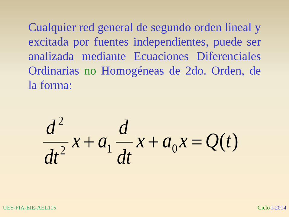
Cualquier red general de segundo orden lineal y

excitada por fuentes independientes, puede ser

analizada mediante Ecuaciones Diferenciales

Ordinarias no Homogéneas de 2do. Orden, de

la forma:

)(012

2

tQxaxdt

dax

dt

d


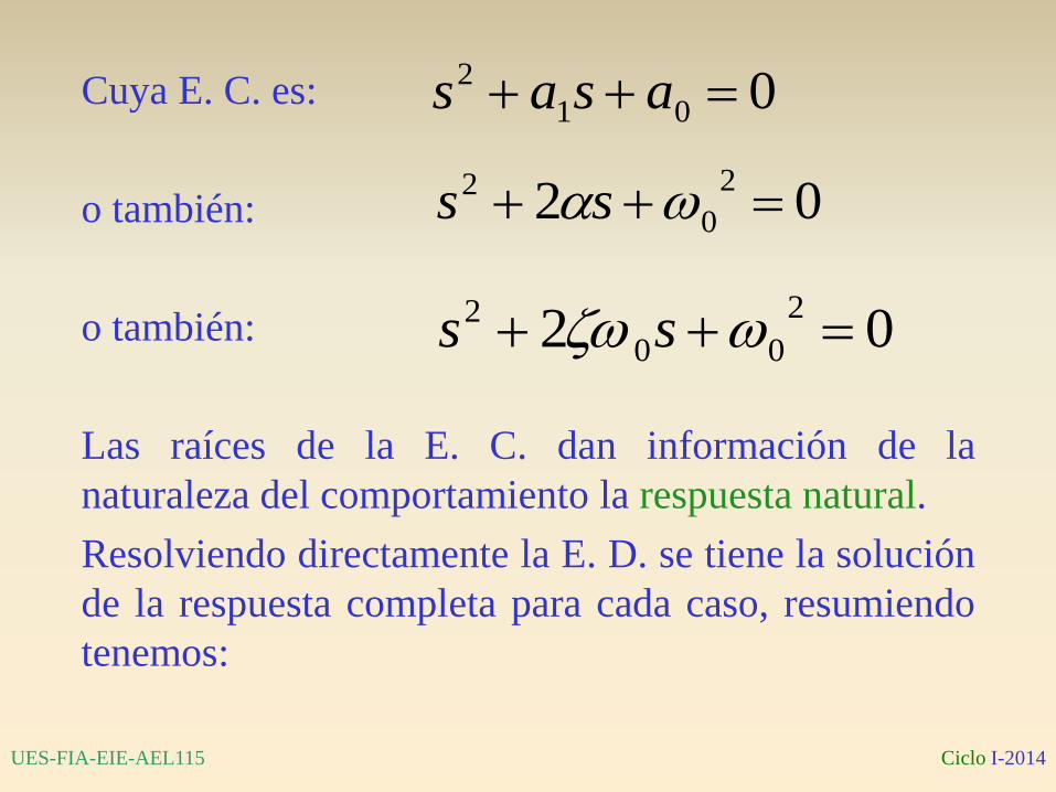
Cuya E. C. es:

o también:

o también:

Las raíces de la E. C. dan información de la

naturaleza del comportamiento la respuesta natural.

Resolviendo directamente la E. D. se tiene la solución

de la respuesta completa para cada caso, resumiendo

tenemos:

001

2 asas

022

0

2 ss

022

00

2 ss


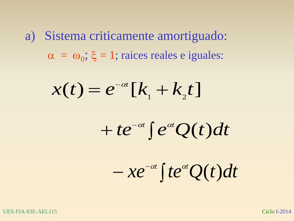
a) Sistema criticamente amortiguado:

= 0; = 1; raices reales e iguales:

][)(21tkketx t

dttQete tt )(

dttQtexe tt )(


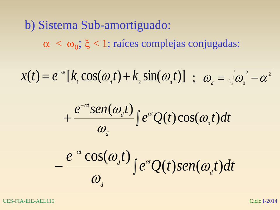
b) Sistema Sub-amortiguado:

< 0; < 1; raíces complejas conjugadas:

)]sin()cos([)(21

tktketxdd

t 22

0 ;

d

dtttQetsene

d

t

d

d

t

)cos()()(

dttsentQete

d

t

d

d

t

)()()cos(


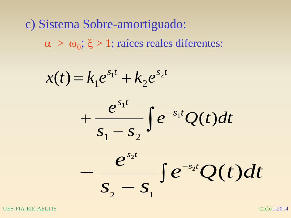
c) Sistema Sobre-amortiguado:

> 0; > 1; raíces reales diferentes:

tstsekektx 21

21)(

dttQess

e tsts

)(1

1

21

dttQess

e ts

ts

)(2

2

12


1) Evaluar la solución de la respuesta completa

en t = t0+ obteniendo una ecuación en

términos de k1 y k2

Similar a las redes RLC sin fuentes, para todos

los casos anteriores, en la solución de la

respuesta completa deben calcularse las

constantes k1 y k2 las cuales están sujeta a las

condiciones iniciales o de frontera de la red en

el instante de tiempo t = t0+, para lo cual se

hacen los pasos siguientes:


2) Derivar la solución de la respuesta completa

y evaluarla en t = t0+ obteniendo otra

ecuación en términos de k1 y k2

3) Encontrar las condiciones de frontera de la

red en t = t0+ para x(t0

+) y la primer derivada

x´(t0+) y sustituirlas en las ecuaciones de los

pasos anteriores para resolver la matriz de

2x2 y determinar las constantes k1 y k2.


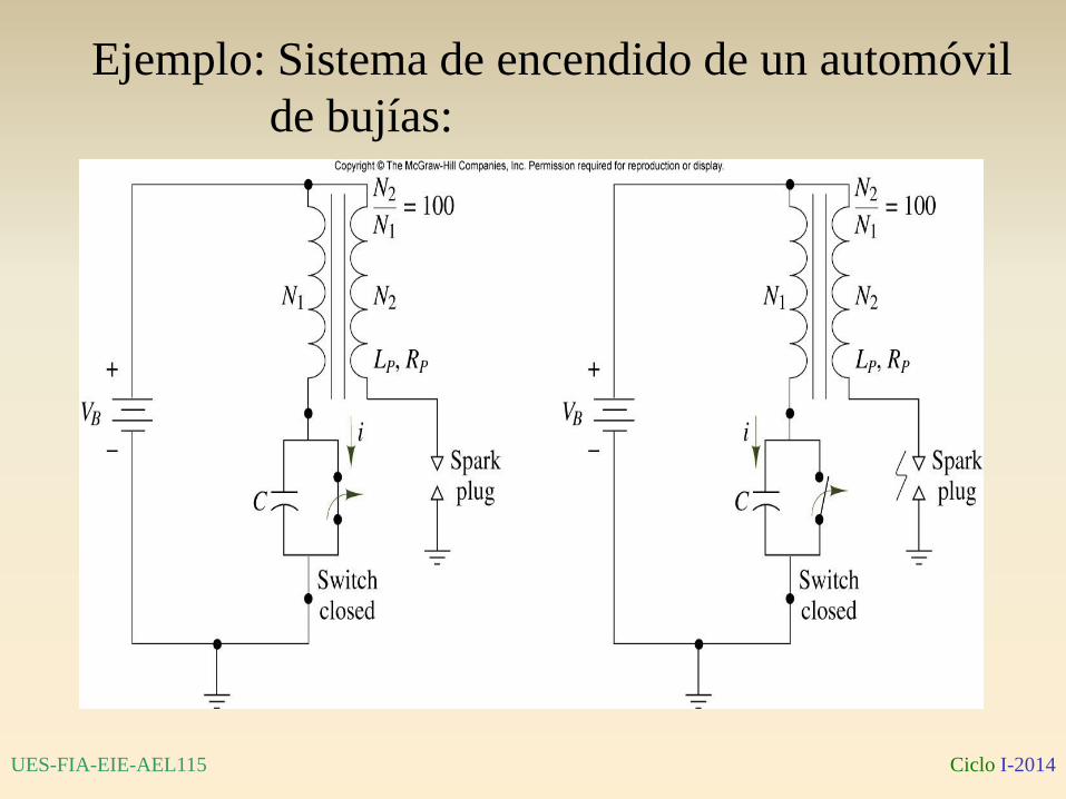
Figure 5.56

Ejemplo: Sistema de encendido de un automóvil

de bujías:


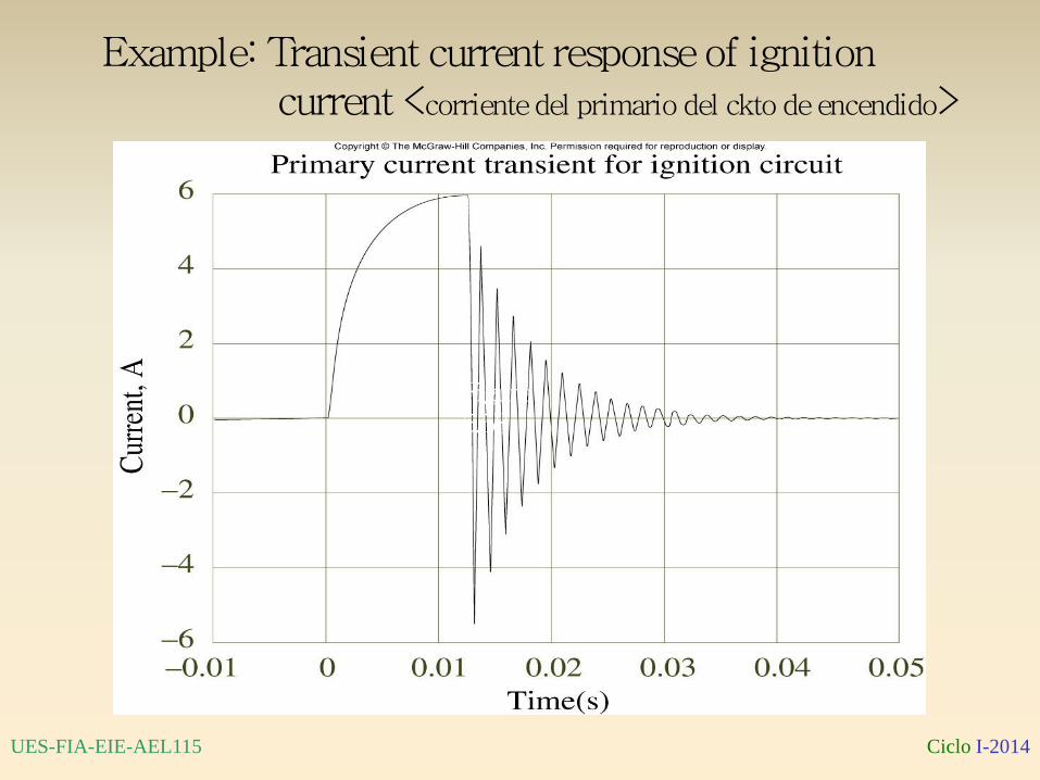
Figure 5.58

Example: Transient current response of ignition current <corriente del primario del ckto de encendido>


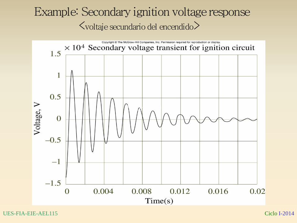
Figure 5.59

Example: Secondary ignition voltage response <voltaje secundario del encendido>


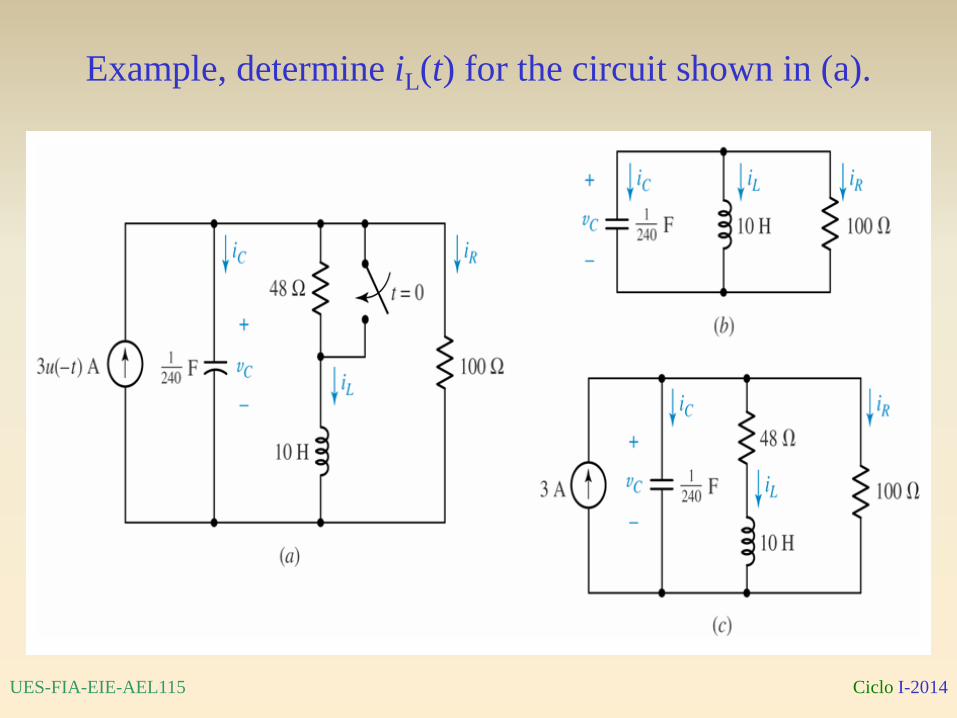
Fig. 9.11 Circuit from

Example 9.2.

Example, determine iL(t) for the circuit shown in (a).


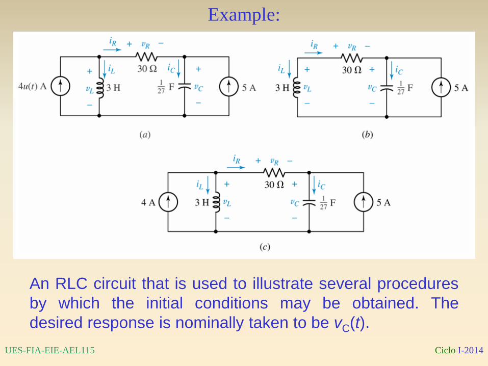
Fig. 9.18 An RLC circuit that

is used to illustrate several

procedures by which the

initial conditions may be

obtained. The desired

response is nominally taken

to be vC(t).

An RLC circuit that is used to illustrate several procedures

by which the initial conditions may be obtained. The

desired response is nominally taken to be vC(t).

Example:

Documents

2-10 Redes RLC