304 Chapter 4 Laplace Transform Methods

1 7. F(s) = --­s (s - 3)

1 9. F (s) = (S2 + 9)2

S2 11 . F(s) = (S2 + 4)2

S 13. F(s) = ------=--­(S - 3 ) (S2 + 1 )

1 8. F (s) = S (S2 + 4)

1 10. F (s) = S2 (S2 + k2)

1 12. F (s) = ----:-::----:-------::::­S (S2 + 4s + 5)

s 14. F (s) = -,-----::-­S4 + 5s2 + 4

In Problems 15 through 22, apply either Theorem 2 or Theo­rem 3 to find the Laplace transform of f(t) . 15. f(t) = t sin 3t 16. f (t) = t2 cos 2t 17. f (t) = te2I cos 3t 18. f (t) = te-l sin2 t

sin t f ) 1 - cos 2t 19. f(t) = - 20. (t = ---t t

e31 - 1 el - e-I 21. f(t) = -- 22. f (t) = --t t Find the inverse transforms of the functions in Problems 23 through 28.

s - 2 23. F(s) = In -­

s + 2 S2 + 1

25. F(s) = In ----­(s + 2) (s - 3)

27. F(s) = In ( 1 + s12 )

S2 + 1 24. F (s) = In -2--s + 4

3 26. F (s) = tan- I

-­

s + 2

28 F (s) _ s

• - (S2 + 1 )3

In Problems 29 through 34, transform the given differential equation to find a nontrivial solution such that x (0) = O. 29. tx" + (t - 2)x' + x = 0 30. tx" + (3t - l )x' + 3x = 0 31. tx" - (4t + l )x' + 2(2t + l )x = 0 32. tx" + 2(t - l )x' - 2x = 0 33. tx" - 2x' + tx = 0 34. tx" + (4t - 2)x' + ( l 3t - 4)x = 0 35. Apply the convolution theorem to show that

£- 1 { 1 yS } = 2� {.Ii e-u2 du = elerf.Jt. (s - l ) s y n Jo (Suggestion: Substitute u = v't .)

In Problems 36 through 38, apply the convolution theorem to derive the indicated solution x (t ) of the given differential equation with initial conditions x (0) = x ' (0) = o.

1 1 1 36. x" + 4x = f(t) ; x (t ) = - f(t - .) sin 2. d. 2 0

37. x" + 2x' + x = f(t) ; x (t) = 11 u-r f(t - .) d-c 38. x" + 4x' + 1 3x = f(t) ;

x (t ) = - f (t - .)e-2r sin 3. d. 1 1 1 3 0

Termwise Inverse Transformation of Series

In Chapter 2 of Churchill 's Operational Mathematics, thefol­lowing theorem is proved. Suppose that f (t ) is continuous for t ;?; 0, that f (t) is of exponential order as t � +00, and that

00 an F (s) = L sn+k+ 1 n=O

where 0 � k < 1 and the series converges absolutely for s > c. Then

00 an tn+k f (t ) = � r (n + k + 1 ) ' Apply this result in Problems 39 through 41. 39. In Example 5 it was shown that

C C ( 1 ) - 1 /2 £ { Jo (t ) } = .JS2+T = - 1 + 2" S2 + 1 s s

Expand with the aid of the binomial series and then com­pute the inverse transformation term by term to obtain

Finally, note that Jo (O) = 1 implies that C = 1 . 40. Expand the function F (s) = S- I /2e- l /s in powers of S- I

to show that

41. Show that

£- 1 { _I_e- l /s } = _1_ cos 2.Jt. yS .fiit

£- 1 { �e- I /s } = Jo (2.Jt) .

Mathematical models of mechanical or electrical systems often involve functions with discontinuities corresponding to external forces that are turned abruptly on or off. One such simple on-off function is the unit step function that we introduced in

x

a FIGURE 4.5.1. The graph of the unit step function at t = a .

a FIGURE 4.5.2. Translation of J (t) a units to the right.

4.5 Periodic and Piecewise Continuous I nput Functions 305

Section 4. 1 . Recall that the unit step Junction at t = a is defined by

1 0 if t < a, ua (t) = u (t - a) = ' f > l i t = a .

( 1 )

The notation Ua (t) indicates succinctly where the unit upward step in value takes place (Fig. 4.5 . 1 ) , whereas u (t - a) connotes the sometimes useful idea of a "time delay" a before the step is made.

In Example 8 of Section 4. 1 we saw that if a � 0, then

e-as "c {u (t - a) } = - .

s (2)

Because "c {u (t ) } = l is , Eg. (2) implies that multiplication of the transform of u (t) by e-as corresponds to the translation t --+ t -a in the original independent variable. Theorem 1 tells us that this fact, when properly interpreted, is a general property of the Laplace transformation.

TH EOREM 1 Translation on the '-Axis

If "cU(t ) } exists for s > c, then

"c{u (t - a)J(t - a) } = e-as F (s)

and

for s > c + a .

Note that

"c-l {e-as F(s) } = u (t - a)J(t - a)

u (t - a)J(t - a) = 1 ° J (t - a) if t < a, if t � a .

(3a)

(3b)

(4)

Thus Theorem 1 implies that "c-l {e-as F (s ) } is the function whose graph for t � a is the translation by a units to the right of the graph of J (t) for t � 0. Note that the part (if any) of the graph of J(t) to the left of t = ° is "cut off" and is not translated (Fig. 4.5 .2) . In some applications the function J(t) describes an incoming signal that starts arriving at time t = 0. Then u (t - a)J (t - a) denotes a signal of the same "shape" but with a time delay of a, so it does not start arriving until time t = a.

ProoJoJ Theorem 1: From the definition of "cU(t) } , we get

The substitution t = r + a then yields

e-as F (s) = 100 e-st J(t - a) dt .

306 Cha pter 4 Laplace Tra nsform Methods

Example 1

Exa mple 2

From Eg. (4) we see that this is the same as

e-as F(s) = 100 e-st u (t - a)f(t - a) dt = £(u (t - a)f(t - a ) } ,

because u (t - a )f(t - a) = ° for t < a . This completes the proof of Theorem 1 . ...

With f(t ) = 4 t2, Theorem 1 gives

£- 1 _ = u (t - a) - (t _ a)2 = { e-S } 1 1 0 s3 2 4 (t - a)2

if t < a , if t � a

Find £(g(t ) } if

if t < 3 ,

i f t � 3 (Fig. 4.5 .4).

(Fig. 4.5 .3) .

•

Solution Before applying Theorem 1 , we must first write g (t) in the form u (t - 3)f (t - 3) .

Example 3

a

The function f(t) whose translation 3 units to the right agrees (for t � 3) with g (t) = t2 is f(t ) = (t + 3)2 because f(t - 3) = t2 . But then

2 6 9 F(s) = £ {t2 + 6t + 9 } = 3" + 2" + - ,

s s s so now Theorem 1 yields

( 2 6 9) £ (g (t ) } = £ (u (t - 3)f (t - 3 ) } = e-3s F(s) = e-3s 3" + 2" + - . s s s

Find £(f (t ) } if

I (t ) = l�s 2t

x

20

1 5

\0

5

2 3

if O � t < 2rr ,

if t � 2rr

4

(Fig. 4 .5 .5) .

x

•

3n: t

FIGURE 4.5.3. The graph of the inverse transfonn of Example I .

FIGURE 4.5.4. The graph of the function g (t ) of Example 2.

FIGURE 4.5.5. The function f (t) of Examples 3 and 4

4.5 Periodic and Piecewise Continuous I nput Functions 307

Solution We note first that

Exa m ple 4

f (t ) = [ 1 - u (t - 2Jl') ] cos 2t = cos 2t - u (t - 2Jl') cos 2(t - 2rr)

because of the periodicity of the cosine function. Hence Theorem 1 gives

s ( 1 - e-2rrs ) £ { f (t ) } = £ {cos 2t } - e-2rrs £ {cos 2t } = 2 • •

s + 4

• • ___ _ __ � � _�� __ M __ � _ M ___ � ____ _ � _ _ _ N __ � " __ N � _ N _ __ N�_ _ _

A mass that weighs 32 lb (mass m = 1 slug) is attached to the free end of a long, light spring that is stretched 1 ft by a force of 4 lb (k = 4 Ib/ft). The mass is initially at rest in its equilibrium position. Beginning at time t = 0 (seconds), an external force f (t ) = cos 2t is applied to the mass, but at time t = 2rr this force is turned off (abruptly discontinued) and the mass is allowed to continue its motion unimpeded. Find the resulting position function x (t ) of the mass .

Solution We need to solve the initial value problem

xl! + 4x = f (t ) ; x (O) = x' (O) = 0,

where f(t ) is the function of Example 3. The transformed equation is

so

Because

s ( 1 - e-2rrS) (s2 + 4)X (s ) = F(s) = 2 ' s + 4

- 1 { S } 1 . 2 £ 2 2 = 4 t sm t

(s + 4)

by Eq. ( 1 6) of Section 4 .3 , it follows from Theorem 1 that

H ,------,---.------,-----, x (t ) = i t sin 2t - u (t - 2Jl') · i (t - 2Jl') sin 2(t - 2rr)

= i [t - u (t - 2Jl') . (t - 2Jl') ] sin 2t . x = H/2

X = -H/2

2H

FIGURE 4.5.6. The graph of the function x (t ) of Example 4.

If we separate the cases t < 2Jl' and t � 2Jl' , we find that the position function may be written in the form l i t sin 2t

x (t ) = !Jl' sin 2t

if t < 2Jl' ,

if t � 2Jl' .

As indicated by the graph of x (t ) shown in Fig. 4.5 .6, the mass oscillates with circular frequency w = 2 and with linearly increasing amplitude until the force is removed at time t = 2Jl' . Thereafter, the mass continues to oscillate with the same frequency but with constant amplitude Jl' /2. The force F (t) = cos 2t would produce pure resonance if continued indefinitely, but we see that its effect ceases immediately at the moment it is turned off. •

308 Cha pter 4 Laplace Transform Methods

Exa m ple 5

Solution

R

FIGURE 4.5.7. The series RLC circuit of Example 5 .

If we were to attack Example 4 with the methods of Chapter 2 , we would need to solve one problem for the interval 0 � t < 2n and then solve a new problem with different initial conditions for the interval t � 2n . In such a situation the Laplace transform method enjoys the distinct advantage of not requiring the solution of different problems on different intervals .

Consider the RLC circuit shown in Fig. 4.5 .7, with R = 1 1 0 n, L = 1 H, C = 0.001 F, and a battery supplying Eo = 90 V. Initially there is no current in the circuit and no charge on the capacitor. At time t = 0 the switch is closed and left closed for 1 second. At time t = 1 it is opened and left open thereafter. Find the resulting current in the circuit.

We recall from Section 2.7 the basic series circuit equation

di . 1 L - + Rl + -q = e (t) ;

dt C (5)

we use lowercase letters for current, charge, and voltage and reserve uppercase let­ters for their transforms. With the given circuit elements, Eq. (5) is

di . dt

+ l l Ol + 1 000q = e (t ) , (6)

where e (t) = 90[ 1 - u (t - 1 ) ] , corresponding to the opening and closing of the switch.

In Section 2.7 our strategy was to differentiate both sides of Eq. (5), then apply the relation

. dq l = -dt

to obtain the second-order equation

d2i di 1 . , L - + R - + -l = e (t ) .

dt2 dt C

(7)

Here we do not use that method, because e' (t ) = 0 except at t = 1 , whereas the jump from e (t) = 90 when t < 1 to e (t) = 0 when t > 1 would seem to require that e'( l ) = - 00 . Thus e'(t) appears to have an infinite discontinuity at t = 1 . This phenomenon will be discussed in Section 4.6. For now, we will simply note that it is an odd situation and circumvent it rather than attempt to deal with it here.

To avoid the possible problem at t = 1 , we observe that the initial value q (0) = 0 and Eq. (7) yield, upon integration,

q (t ) = 11 i (r: ) dr:.

We substitute Eq. (8) in Eq. (5) to obtain

di 1 11 L - + Ri + - i (r:) dr: = e (t) . dt C 0

(8)

(9)

This is the integrodifferential equation of a series RLC circuit; it involves both the integral and the derivative of the unknown function i (t ) . The Laplace transform method works well with such an equation.

4.5 Periodic and Piecewise Continuous I nput Functions 309

In the present example, Eq. (9) is

Because

di t dt +

1 10i + 1 000 10 i (r ) dr = 90 [ 1 - u (t - 1 ) ] .

{ t } / (s) £. 10

i (r ) dr = -s-

(10)

by Theorem 2 of Section 4.2 on transforms of integrals, the transformed equation is

/ (s) 90 s / (s) + 1 I 0/ (s) + 1 000- = - ( 1 - e-S ) . s s

We solve this equation for / (s) to obtain

But

so we have

90( 1 - e-S ) / (s ) =

s2 + l I Ds + 1 000 ·

90 1 1 -::------ = -- - ----:-s2 + 1 1 0s + 1 000 s + 1 0 s + 100 '

1 1 -s ( 1 1 ) / (s) = s + 1 0

-s + 1 00

- e s + 10

-s + 100

.

We now apply Theorem 1 with f(t) = e- 101 - e- 1OOI ; thus the inverse transform is

i (t ) = e- IOI - e- IOOI - u (t - 1 ) [e- IO(I- l ) _ e- IOO(I- l ) ] .

After we separate the cases t < 1 and t � 1 , we find that the current in the circuit is given by

e - e 1 - 101 - 1001 i (t ) = e- IOI _ e- IO(I- l ) _ e- IOOI + e- 100(I- l )

if t < 1 , if t � 1 .

The portion e- IOI - e- IOOI of the solution would describe the current if the switch were left closed for all t rather than being open for t � 1 . •

31 0 Chapter 4 Laplace Transform Methods

I I I I

�p� FIGURE 4.5.8. The graph of a function with period p .

Transforms of Periodic Functions

Periodic forcing functions in practical mechanical or electrical systems often are more complicated than pure sines or cosines. The nonconstant function f(t) defined for t � 0 is said to be periodic if there is a number p > 0 such that

f(t + p) = f(t) ( 1 1 )

for all t � O. The least positive value of p (if any) for which Eq. ( 1 1 ) holds is called the period of f. Such a function is shown in Fig. 4.5 .8 . Theorem 2 simplifies the computation of the Laplace transform of a periodic function.

TH EOREM 2 Transforms of Periodic Functions

Let f(t) be periodic with period p and piecewise continuous for t � O. Then the transform F(s) = £{f(t ) } exists for s > 0 and is given by

F(s) = e-st f(t) dt . 1 loP

1 - e-PS 0

Proof: The definition of the Laplace transform gives

100 00 l (n+ l )p F(s) = e-st f(t) dt = L e-st f(t) dt . o n=O np

( 1 2)

The substitution t = r + np in the nth integral following the summation sign yields

l (n+ l )p lP lP e-st f(t) dt = e-s (r+np) f(r + np) dr = e-nps e-sr f(r ) dr � 0 0

because f(r + np) = f(r) by periodicity. Thus

Consequently,

F(s) = f (e-nps lP e-sr f(r) dr) n=O 0

= ( 1 + e-Ps + e-2ps + . . . ) loP e-sr f(r ) dr .

F (s) = 1 ( P e-sr f(r ) dr .

1 - e-PS 10 We use the geometric series

1 2 3 -- = I + x + x + x + . . . , I - x

with x = e-Ps < 1 (for s > 0) to sum the series in the final step. Thus we have derived Eq. ( 1 2) . ...

The principal advantage of Theorem 2 is that it enables us to find the Laplace transform of a periodic function without the necessity of an explicit evaluation of an improper integral .

Exa mple 6

f(t ) e---o e---o .... . . .

a 2a 3a 4a 5a 6a - I e---o e---o e---o

FIGURE 4.5.9. The graph of the square-wave function of Example 6.

Exa m ple 7 g(t)

... a 2a 3a 4a 5a 6a

FIGURE 4.5.10. The graph of the triangular-wave function of Example 7.

Exa m ple 8

4.5 Periodic and Piecewise Continuous Input Functions 31 1

Fig�re 4.5 .9 shows ihe graph of the square-wave function f(t) = (_ i) [tj�D of period p = 2a ; [x] denotes the greatest integer not exceeding x . By Theorem 2 the Laplace transform of f(t ) is

Therefore,

1 12a F (s) = 2 e-st f(t) dt

1 - e- as 0

= 1 ( r e-st dt + 12a

(- l )e-st dt) 1 - e-2as Jo a

= 1 ( [_ !e-stJ a _ [_ !e-stJ 2a)

1 - e-2as s 0 S a

1 - e-as F(s ) = ---­

s ( 1 + e-as )

I -as - e

eas/2 - e-as/2 1 as = = - tanh - . s (eas/2 + e-as/2 ) S 2

( 1 3a)

( 1 3b)

•

Figure 4.5 . 1 0 shows the graph of a triangular-wave function g(t) of period p = 2a . Because the derivative g' (t) is the square wave function of Example 6, it follows from the formula in ( l 3b) and Theorem 2 of Section 4.2 that the transform of this triangular-wave function is

F (s ) 1 as G(s ) = -- = - tanh - .

s s2 2

._-- _ . . . _ . . . . . . _ . . _ . . _ _ . ---_ . . _ . . . _ . _ - - -_._- - - _ . . . _ . . _---_.

( 14)

•

Consider a mass-spring-dashpot system with m = 1 , c = 4, and k = 20 in ap­propriate units . Suppose that the system is initially at rest at equilibrium (x (O) = x' (0) = 0) and that the mass is acted on beginning at time t = 0 by the external force f(t) whose graph is shown in Fig. 4 .5 . 1 1 : the square wave with amplitude 20 and period 2rr . Find the position function f(t ) .

Solution The initial value problem is

x" + 4x' + 20x = f(t ) ; x (O) = x' (O) = O.

The transformed equation is

S2X (S) + 4s X (s ) + 20X (s) = F (s ) . ( 1 5)

31 2 Chapter 4 La place Transform Methods

.f(t) 20 ..---<? ..---<? .......-0

I I I I I

1t 21t 31t 41t S1t 61t I I I I I I I I I I I I I I I I I I I I I I I I -20 .........0 � � FIGURE 4.5.11 . The graph of the external-force function of Example 8.

From Example 6 with a = :rr we see that the transform of f (t) is

so that

20 1 - e-:n:s F(s) = - · --­

s 1 + e-:n:s

20 = - ( 1 - e-:n:S ) ( 1 _ e-:n:s + e-2:n:s _ e-3:n:s + . . . ) s

20 = - ( 1 - 2e-:n:s + 2e-2:n:s _ 2e-3:n:s + . . . ) , s

20 40 00 F(s ) = - + - L(- l )n e-n:n:s . s S n=1

Substitution of Eq. ( 1 6) in Eq. ( 1 5) yields

X (s) _ F(s) - s2 + 4s + 20

( 16)

20 00 20e-n:n:s = s [ (s + 2)2 + 1 6]

+ 2 � (_ l )n s [ (s + 2)2 + 1 6] " ( 17)

From the transform in Eq. (8) of Section 4.3 , we get

£- 1 { 20 } = 5e-2t sin 4t (s + 2)2 + 16 '

so by Theorem 2 of Section 4.2 we have

g (t ) = £- 1 { 202

} = r 5e-2, sin 4r dr . s [ (s + 2) + 1 6] 10

U sing a tabulated formula for J eat sin bt d t , we get

g (t) = 1 - e-2t (cos 4t + 4 sin 4t) = 1 - h (t) ,

where

h (t ) = e-2t (cos 4t + 4 sin 4t) .

( 1 8)

( 1 9)

Now we apply Theorem 1 to find the inverse transform of the right-hand term in Eq. ( 1 7) . The result is

00 x (t ) = g (t ) + 2 L(- ltu (t - n:rr )g (t - n:rr ) , (20)

n=1

and we note that for any fixed value of t the sum in Eq. (20) is finite. Moreover,

g (t - n:rr ) = 1 - e-2(t-n:n:) [cos 4(t - n:rr ) + 4 sin 4(t - n:rr ) ]

= 1 - e2n:n: e-2t (cos 4t + 4 sin 4t) .

4.5 Periodic and Piecewise Continuous I nput Functions 31 3

Therefore,

g (t - mr) = 1 - e2n:n: h (t ) .

Hence i f 0 < t < Jr, then x (t ) = 1 - h (t ) .

I f Jr < t < 2Jr , then

x (t ) = [ 1 - h (t) ] - 2 [ 1 - e2:n: h (t ) ] = - 1 + h (t) - 2h (t) [ 1 - e2:n:] .

If 2Jr < t < 3Jr, then

x (t) = [ 1 - h (t) ] - 2 [ 1 - e2:n:h (t)] + 2 [ 1 - e4:n:h (t)] = 1 + h (t ) - 2h (t) [ 1 - e2:n: + e4:n: ] .

The general expression fo( nJr < t < (n + 1 )Jr is

x (t ) = h (t) + (_ 1 )n - 2h (t ) [ 1 - e2:n: + . . . + (_ 1 )ne2n:n: ]

1 + (_ Ite2(n+ l ):n: = h (t) + (- It - 2h (t) 2 ' I + e :n:

(2 1 )

(22)

which we obtained with the aid of the familiar formula for the sum of a finite ge­ometric progression. A rearrangement of Eq. (22) finally gives, with the aid of Eq. ( 1 9),

e2:n: - 1 x (t ) = 2 e-2t (cos 4t + t sin 4t) + (_ I )n

e :n: + 1 2 . (_ 1 )ne2:n:

- e-2(t-n:n:) (cos 4t + ! sin 4t) e2:n: + 1 2

for nJr < t < (n + I )Jr . The first term in Eq. (23) is the transient solution

(23)

Xtr(t) � (0.9963)e-2t (cos 4t + t sin 4t) � ( 1 . 1 1 39)e-2t cos (4t - 0.4636) . (24)

The last two terms in Eq. (23) give the steady periodic solution xsp . To investigate it, we write r = t - nJr for t in the interval nJr < t < (n + I)Jr . Then

xsp (t) = (_ 1 )n [ 1 - 22e2:n:

e-2r (cos 4r + t sin 4r)] e :n: + 1 (25) � (_ I )n [ 1 - (2.23 I 9)e-2r cos (4r - 0.4636)] .

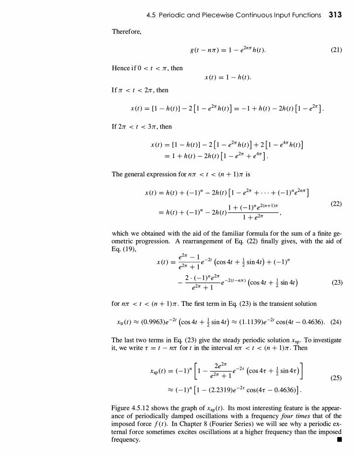
Figure 4.5 . 1 2 shows the graph of xsp (t) . Its most interesting feature is the appear­ance of periodically damped oscillations with a frequency four times that of the imposed force f(t) . In Chapter 8 (Fourier Series) we will see why a periodic ex­ternal force sometimes excites oscillations at a higher frequency than the imposed frequency. •

3 1 4 Chapter 4 Laplace Transform Methods

- I

- I + (2 .23)e -2(t - It) II

I V\

I I \

I I I I

I _ I - (2.23)e -2(t - It) I

/ /

FIGURE 4.5.12. The graph of the steady periodic solution for Example 8 ; note the "periodically damped" oscillations with frequency four times that of the imposed force.

IID,. Problems Find the inverse Laplace transform f (t) of each function given in Problems 1 through 10. Then sketch the graph of f.

e-3s 1. F(s) = -2 S

e-S 3. F(s) = --

2 s + e-1t"'

5. F(s) = S2 + 1 1 - e-21ts

7. F(s) = S2 + 1 s ( l + e-3s )

9. F(s) = 2 2 S + n

e-S _ e-3s 2. F(s) = 2 S

e-S _ e2-2s 4. F(s) = ---­s - 1

se-S 6. F(s) = -2--2 S + n

8. F(s) = sO - e-2s ) S2 + n2

2s (e-1tS _ e-21t"' ) 10. F(s) = S2 + 4

Find the Laplace transforms of the functions given in Problems 11 through 22. 11. J(t) = 2 if 0 � t < 3 ; f(t) = 0 if t � 3 12. J(t) = 1 if 1 � t � 4; f(t) = 0 if t < 1 or if t > 4 13. J(t) = sin t if 0 � t � 2n ; J(t) = O if t > 2n 14. J(t) = cos m if 0 � t � 2; J(t) = 0 if t > 2 15. J(t) = sin t if 0 � t � 3n ; J(t) = O if t > 3n 16. J(t) = sin 2t if n � t � 2n ; f (t) = 0 if t < n or if

t > 2n 17. J(t) = sin m if 2 � t � 3 ; J (t) = O if t < 2 0r if t > 3 18. f(t) = cos �m if 3 � t � 5 ; J(t) = O if t < 3 or if t > 5 19. f(t) = 0 if t < 1 ; f(t) = t if t � 1 20. f(t) = t if t � 1 ; J(t) = 1 if t > 1 21. J(t) = t if t � 1 ; J(t) = 2 - t if 1 � t � 2; f(t) = 0 if

t > 2 22. J(t) = t3 if 1 � t � 2; J(t) = 0 if t < I or if t > 2

23. Apply Theorem 2 with p = 1 to verify that el{ l } = lis . 24. Apply Theorem 2 to verify that el{cos kt } = sl(s2 + k2) . 25. Apply Theorem 2 to show that the Laplace transform of

the square-wave function of Fig. 4.5 . 1 3 is

1 elU(t) } = s ( l + e-aS )

-1 -1 -1 -1 -I -I I I I I

a 2a 3a 4a 5a 6a

FIGURE 4.5.13. The graph of the square-wave function of Problem 25 .

26. Apply Theorem 2 to show that the Laplace transform of the sawtooth function J(t) of Fig. 4.5 . 14 is

1 e-as F(s) = - - . as2 sO - e-as )

f(t )

a 2a 3a 4a 5a 6a

FIGURE 4.5.14. The graph of the sawtooth function of Problem 26.

4.5 Periodic and Piecewise Continuous I nput Functions 31 5

27. Let g (t) be the staircase function of Fig. 4.S . 1 S . Show that g (t) = (t / a) - f (t ) , where f is the sawtooth function of Fig. 4.S . 14 , and hence deduce that

e-as £ {g (t) } = s ( l _ e-aS )

g(t ) 4 , • • •

I I 3 r---' I I 2 r---' I I

r---'

a 2a 3a 4a t FIGURE 4.5.15. The graph of the staircase function of Problem 27.

28. Suppose that f (t) is a periodic function of period 2a with f (t) = t if 0 ;;:; t < a and f (t) = 0 if a ;;:; t < 2a . Find £ {f(t) } .

29. Suppose that f(t) is the half-wave rectification of sin kt , shown in Fig. 4.S . 1 6. Show that

k £ {f(t) } = (S2 + P) ( l _ e-"sfk )

f\ 2" 3" T T

FIGURE 4.5.16. The half-wave rectification of sin kt .

30. Let g (t) = u (t - n/k)f(t - n/k) , where f(t) is the function of Problem 29 and k > O. Note that h (t) = f(t) + g(t) is the full-wave rectification of sin kt shown in Fig. 4.S . 17 . Hence deduce from Problem 29 that

k ns £ {h (t ) } = S2 + k2 coth 2k ·

!! � � k k k

FIGURE 4.5.17. The full-wave rectification of sin kt .

In Problems 31 through 35, the values of mass m, spring con­stant k, dashpot resistance c, and force f (t) are given for a

mass-spring-dashpot system with external forcing function. Solve the initial value problem

mx" + cx' + kx = f(t ) , x (O) = x' (O) = 0

and construct the graph of the position function x (t) . 31. m = 1 , k = 4, c = 0; f(t) = 1 if 0 ;;:; t < n, f(t) = 0 if

t � n 32. m = 1 , k = 4, c = S ; f(t) = 1 if 0 ;;:; t < 2, f(t) = 0 if

t � 2 33. m = 1 , k = 9, c = 0; f(t) = sin t if 0 ;;:; t ;;:; 2n ,

f (t) = 0 if t > 2n 34. m = 1 , k = 1 , c = 0; f(t) = t if 0 ;;:; t < 1 , f(t) = 0 if

t � 1 35. m = 1 , k = 4, c = 4; f(t) = t if 0 ;;:; t ;;:; 2, f(t) = 0 if

t > 2

In Problems 36 through 40, the values of the elements of an RLC circuit are given. Solve the initial value problem

di 1 l' L- + Ri + - i (r) dr = e(t) ; dt C 0

with the given impressed voltage e(t).

i (O) = 0

36. L = 0, R = 100, C = 10-3 ; e(t) = 100 if 0 ;;:; t < 1 ; e(t) = 0 if t � 1

37. L = 1 , R = 0, C = 10-4 ; e(t) = 100 if 0 ;;:; t < 2n ; e(t) = 0 if t � 2n

38. L = 1 , R = 0, C = 10-4 ; e(t) = 100 sin lOt if 0 ;;:; t < n ; e(t) = 0 if t � n

39. L = 1 , R = lS0, C = 2 x 10-4 ; e(t) = lOOt if 0 ;;:; t < I ; e(t) = 0 i f t � 1

40. L = 1 , R = 100, C = 4 x 10-4 ; e(t) = SOt if 0 ;;:; t < 1 ; e(t) = 0 if t � 1

In Problems 41 and 42, a mass-spring-dashpot system with external force f(t) is described. Under the assumption that x (O) = x' (O) = 0, use the method of Example 8 to find the transient and steady periodic motions of the mass. Then con­struct the graph of the position function x (t) . If you would like to check your graph using a numerical DE solver, it may be useful to note that the function

f(t) = A [2u «t - n) (t - 2n) (t - 3n) . (t - 4n) (t - Sn) (t - 6n )) - 1]

has the value +A if 0 < t < n, the value -A ifn < t < 2n, and so forth, and hence agrees on the interval [0, 6n] with the square-wave function that has amplitude A and period 2n. (See also the definition of a square-wave function in terms of sawtooth and triangular-wave functions in the application ma­terialfor this section. ) 41. m = 1 , k = 4, c = 0; f(t) is a square-wave function with

amplitude 4 and period 2n . 42. m = 1 , k = 10, c = 2; f(t) is a square-wave function

with amplitude 1 0 and period 2n .

3 1 6 Chapter 4 Laplace Transform Methods

lID !1l1::pulses and Delta Functions

x I-- e -----j

r IT I I I I : Area = ! : � I I I I I I I I

a a + e FIGURE 4.6.1. The graph of the impulse function da ,< (t ) .

Consider a force f(t ) that acts only during a very short time interval a � t � b, with f(t) = 0 outside this interval . A typical example would be the impulsive force of a bat striking a ball-the impact is almost instantaneous. A quick surge of voltage (resulting from a lightning bolt, for instance) is an analogous electrical phenomenon. In such a situation it often happens that the principal effect of the force depends only on the value of the integral

p = lb f (t) dt ( 1 )

and does not depend otherwise on precisely how f (t) varies with time t . The num­ber p in Eq. ( 1 ) is called the impulse of the force f(t) over the interval [a , b] .

In the case of a force f (t) that acts on a particle of mass m in linear motion, integration of Newton's law

yields

d f(t) = mv' (t) = - [mv (t) ] dt

lb d p = - [mv (t ) ] dt = mv(b) - mv (a ) .

a dt (2)

Thus the impulse of the force is equal to the change in momentum of the particle. So if change in momentum is the only effect with which we are concerned, we need know only the impulse of the force; we need know neither the precise function f(t) nor even the precise time interval during which it acts . This is fortunate, because in a situation such as that of a batted ball, we are unlikely to have such detailed information about the impulsive force that acts on the ball.

Our strategy for handling such a situation is to set up a reasonable mathemat­ical model in which the unknown force f(t) is replaced with a simple and explicit force that has the same impulse. Suppose for simplicity that f(t ) has impulse 1 and acts during some brief time interval beginning at time t = a � O. Then we can select a fixed number E > 0 that approximates the length of this time interval and replace f(t) with the specific function

if a � t < a + E , (3)

otherwise.

This is a function of t , with a and E being parameters that specify the time interval [a , a + E ] . If b � a + E , then we see (Fig. 4.6. 1 ) that the impulse of da ,E over [a , b] is

p = lb da , E (t) dt = la+E

! dt = 1 . a a E

Thus da,E has a unit impulse, whatever the number E may be. Essentially the same computation gives

(4)

Function g (t) \

FIGURE 4.6.2. A diagram illustrating how the delta function "sifts out" the value g (a ) .

4.6 Impu lses and Delta Functions 31 7

Because the precise time interval during which the force acts seems unimpor­tant, it is tempting to think of an instantaneous impulse that occurs precisely at the instant t = a . We might try to model such an instantaneous unit impulse by taking the limit as E � 0, thereby defining

(5)

where a � O. If we could also take the limit under the integral sign in Eq. (4), then it would follow that

(6)

But the limit in Eq. (5) gives

if t = a , (7)

if t =1= a .

Obviously, no actual function can satisfy both (6) and (7)-if a function is zero except at a single point, then its integral is not I but zero. Nevertheless, the symbol Da (t) is very useful. However interpreted, it is called the Dirac delta function at a after the British theoretical physicist P. A. M. Dirac ( 1 902-1984), who in the early 1 930s introduced a "function" allegedly enjoying the properties in Eqs . (6) and (7).

Delta Functions as Operators

The following computation motivates the meaning that we will attach here to the symbol Da (t) . If g(t) is continuous function, then the mean value theorem for inte­grals implies that la+€

g(t ) dt = Eg (t ) for some point t in [a , a + E) . I t follows that 100 la+€ 1

lim g (t)da , € (t) dt = lim g (t) . - dt = lim g (t) = g(a) €---+ O 0 €---+ O a E €---+O (8)

by continuity of g at t = a . If Da (t) were a function in the strict sense of the definition, and if we could interchange the limit and the integral in Eq. (8), we therefore could conclude that 100 g(t)Da (t) dt = g(a ) . (9)

We take Eq. (9) as the definition ( ! ) of the symbol Da (t ) . Although we call it the delta function, it is not a genuine function; instead, it specifies the operation

which-when applied to a continuous function g (t)-sifts out or selects the value g (a) of this function at the point a � O. This idea is shown schematically in Fig. 4.6.2. Note that we will use the symbol Da (t) only in the context of integrals such as that in Eq. (9), or when it will appear subsequently in such an integral.

31 8 Chapter 4 Laplace Transform Methods

For instance, if we take g (t) = e-st in Eq. (9) , the result is

We therefore define the Laplace transform of the delta function to be

If we write

£ {8a (t) } = e-as (a � 0) .

8 (t ) = 80 (t) and 8 (t - a) = 8a (t) ,

then ( 1 1 ) with a = 0 gives

£ {8 (t) } = 1 .

( 10)

( 1 1 )

( 12)

( 1 3)

Note that if 8 (t ) were an actual function satisfying the usual conditions for existence of its Laplace transform, then Eq. ( 1 3) would contradict the corollary to Theorem 2 of Section 4. 1 . But there is no problem here; 8 (t ) is not a function, and Eq. ( 1 3) is our definition of £ {8 (t ) } .

Delta Function Inputs

,Now, finally, suppose that we are given a mechanical system whose response x (t) to the external force f(t) is determined by the differential equation

Ax" + Bx' + ex = f(t) . ( 14)

To investigate the response of this system to a unit impulse at the instant t = a, it seems reasonable to replace f(t) with 8a (t) and begin with the equation

Ax" + Bx' + ex = 8a (t) . ( 1 5)

But what is meant by the solution of such an equation? We will call x (t) a solution of Eq. ( 1 5) provided that

x (t) = lim x€ (t) , €-->o ( 1 6)

where x€ (t) is a solution of

Ax" + Bx' + ex = da , € (t) . ( 17)

Because

( 1 8)

is an ordinary function, Eq. ( 1 7) makes sense. For simplicity suppose the initial conditions to be x (O) = x' (O) = O. When we transform Eq. ( 1 7) , writing X€ = £ {x€ } , we get the equation

Exa m ple 1

4.6 Impu lses and Delta Functions 31 9

If we take the limit in the last equation as E ---+ 0, and note that

1 - e-SE lim = 1 E-+O SE

by I 'Hopital ' s rule, we get the equation

(AS2 + Bs + C)X (s) = e-as ,

if X (s) = lim XE (x) . E-+O

( 1 9)

Note that this is precisely the same result that we would obtain if we transformed Eq. ( 1 5) directly, using the fact that £{8a (t ) } = e-as .

On this basis it is reasonable to solve a differential equation involving a delta function by employing the Laplace transform method exactly as if 8a (t) were an ordinary function. It is important to verify that the solution so obtained agrees with the one defined in Eq. ( 1 6) , but this depends on a highly technical analysis of the limiting procedures involved; we consider it beyond the scope of the present discussion. The formal method is valid in all the examples of this section and will produce correct results in the subsequent problem set.

-�-- - --. - --.-- --�.---".� ... -,,- - .� ....

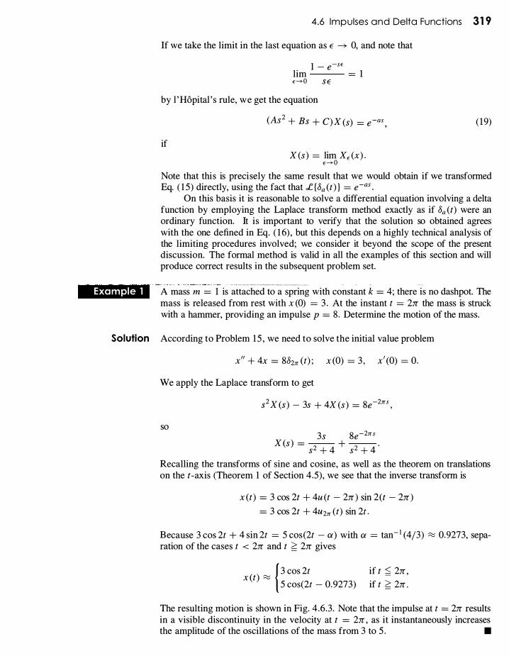
A mass m = 1 is attached to a spring with constant k = 4; there is no dashpot. The mass is released from rest with x (0) = 3 . At the instant t = 217: the mass is struck with a hammer, providing an impulse p = 8 . Determine the motion of the mass.

Solution According to Problem 1 5 , we need to solve the initial value problem

x" + 4x = 8823T (t) ; x (O) = 3 , x' (O) = O.

We apply the Laplace transform to get

so

S2 X (s) - 3s + 4X (s) = 8e-23TS ,

3s 8e-23TS X (s) =

s2 + 4 + s2 + 4 '

Recalling the transforms of sine and cosine, as well as the theorem on translations on the t-axis (Theorem 1 of Section 4.5), we see that the inverse transform is

x (t) = 3 cos 2t + 4u (t - 217:) sin 2(t - 217:) = 3 cos 2t + 4U23T (t) sin 2t .

Because 3 cos 2t + 4 sin 2t = 5 cos (2t - a) with a = tan- 1 (4/3) � 0.9273, sepa­ration of the cases t < 217: and t � 217: gives

( ) 1 3 cos 2t x t � 5 cos(2t - 0.9273)

if t � 217: , if t � 217: .

The resulting motion is shown in Fig. 4.6.3 . Note that the impulse at t = 217: results in a visible discontinuity in the velocity at t = 217: , as it instantaneously increases the amplitude of the oscillations of the mass from 3 to 5 . •

320 Cha pter 4 Laplace Transform Methods

x

a a + E

6

- 6

o

t = 2Jr

2n 4n t

6n

FIGURE 4.6.3. The motion of the mass of Example 1 .

Delta Functions and Step Functions

It is useful to regard the delta function 8a (t) as the derivative of the unit step function ua (t) . To see why this is reasonable, consider the continuous approximation Ua , f (t) to ua (t) shown in Fig. 4.6.4. We readily verify that

Because

FIGURE 4.6.4. Approximation of ua (t) by ua , . (t ) .

an interchange of limits and derivatives yields

Exa mple 2

and therefore

d -ua (t) = 8a (t) = 8 (t - a) . dt

(20)

We may regard this as theformal definition of the derivative of the unit step function, although Ua (t) is not differentiable in the ordinary sense at t = a .

- - - -

We return to the RLC circuit of Example 5 of Section 4.5, with R = 1 1 0 n, L = 1 H, C = 0.001 F, and a battery supplying eo = 90 V. Suppose that the circuit is initially passive-no current and no charge. At time t = 0 the switch is closed and at time t = 1 it is opened and left open. Find the resulting current i (t) in the circuit.

Solution In Section 4.5 we circumvented the discontinuity in the voltage by employing the in­tegrodifferential form of the circuit equation. Now that delta functions are available, we may begin with the ordinary circuit equation

Li" + Ri ' + .!.i = e' (t) . C

In this example we have

e(t) = 90 - 90u (t - 1 ) = 90 - 90u , (t) ,

Exa m ple 3

4.6 Impu lses and Delta Functions 321

so e' (t) = -908 (t - 1 ) by Eq. (20) . Hence we want to solve the initial value problem

i " + HOi ' + 1000i = -908 (t - 1 ) ; i (O) = 0, i ' (O) = 90. (2 1 )

The fact that i ' (0) = 90 comes from substitution of t = 0 in the equation

1 Li ' (t) + Ri (t) + C q (t) = e (t)

with the numerical values i (O) = q (O) = 0 and e (O) = 90. When we transform the problem in (2 1 ), we get the equation

s2 I (s) - 90 + HOsI (s) + 1 000/ (s) = -90e-s .

Hence 90( 1 - e-S ) I (s) =

S2 + HOs + 1 000 This is precisely the same transform I (s ) we found in Example 5 of Section 4.5, so inversion of I (s) yields the same solution i (t) recorded there. •

Consider a mass on a spring with m = k = 1 and x (0) = x' (0) = O. At each of the instants t = 0, :rr , 2:rr , 3:rr , . . . , n:rr , . . . , the mass is struck a hammer blow with a unit impulse. Determine the resulting motion.

Solution We need to solve the initial value problem

x(t )

00 x" + x = I )mr (t) ; x (O) = 0 = x' (O) .

n=O Because £ {8mr (t ) } = e-nrr s , the transformed equation is

so

00 S2X (s) + X (s) = L e-nrrs ,

n=O

00 e-nrrs X (s) = L -2-1 · n=O S +

We compute the inverse Laplace transform term by term; the result is

00 x (t) = L u (t - n:rr ) sin(t - n:rr ) .

n=O Because sin(t - n:rr ) = (_ 1 )n sin t and u (t - n:rr ) = 0 for t < n:rr , we see that if n:rr < t < (n + 1 ):rr , then

x (t) = sin t - sin t + sin t - . . . + (- It sin t ;

that is,

x (t) = losin t if n is even,

if n is odd.

Hence x (t) is the half-wave rectification of sin t shown in Fig. 4.6.5 . The physical explanation is that the first hammer blow (at time t = 0) starts the mass moving to

�I-----'---L-----'-----I.-t the right; just as it returns to the origin, the second hammer blow stops it dead; it rr 2n: 3n: 4n:

FIGURE 4.6.5. The half-wave rectification of sin t .

remains motionless until the third hammer blow starts i t moving again, and so on. Of course, if the hammer blows are not perfectly synchronized then the motion of the mass will be quite different. •

322 Chapter 4 Laplace Tra nsform Methods

Systems Analysis and Duhamel's Principle

Consider a physical system in which the output or response x (t) to the input func­tion f(t) is described by the differential equation

ax" + bx' + ex = f(t ) , (22)

where the constant coefficients a , b, and e are determined by the physical parameters of the system and are independent of f (t) . The mass-spring-dashpot system and the series RLC circuit are familiar examples of this general situation.

For simplicity we assume that the system is initially passive: x (O) = x' (O) = O. Then the transform of Eq. (22) is

so

The function

as2X (s) + bsX (s) + eX (s) = F (s ) ,

F (s) X (s) = 2 = W(s) F(s ) .

as + bs + e

1 W(s) = ---­

as2 + bs + e

(23)

(24)

is called the transfer function of the system. Thus the transform of the response to the input f(t) is the product of W(s) and the transform F(s) .

The function

w(t) = .,c- l rW (s ) } (25)

is called the weight function of the system. From Eq. (24) we see by convolution that

x (t) = lot w(r)f (t - r) dr . (26)

This formula is Duhamel's principle for the system. What is important is that the weight function w(t) is determined completely by the parameters of the system. Once w (t) has been determined, the integral in (26) gives the response of the system to an arbitrary input function f(t ) .

In principle-that i s , via the convolution integral-Duhamel's principle re­duces the problem of finding a system's outputs for all possible inputs to calculation of the single inverse Laplace transform in (25) that is needed to find its weight func­tion. Hence, a computational analogue for a physical mass-spring-dashpot system described by (22) can be constructed in the form of a "black box" that is hard-wired to calculate (and then tabulate or graph, for instance) the response x (t) given by (26) automatically whenever a desired force function f (t) is input. In engineering prac­tice, all manner of physical systems are "modeled" in this manner, so their behaviors can be studied without need for expensive or time-consuming experimentation.

Exa mple 4

4.6 Impu lses and Delta Functions 323

Consider a mass-spring-dashpot system (initially passive) that responds to the ex­ternal force f(t) in accord with the equation x" + 6x' + l Ox = f(t) . Then

1 1 W(s) - - ---=---- s2 + 6s + 10

- (s + 3)2 + l '

so the weight function is w(t) = e-31 sin t . Then Duhamel 's principle implies that the response x (t) to the force f(t) i s

Note that

x (t) = 1 1 e-3, (sin r )f (t - r) dr .

W(s) = 1 = £ {8 (t) } .

as2 + bs + c as2 + bs + c

•

Consequently, it follows from Eq. (23) that the weight function is simply the re­sponse of the system to the delta function input 8 (t ) . For this reason w(t) is some­times called the unit impulse response. A response that is usually easier to measure in practice is the response h (t) to the unit step function u (t ) ; h (t) is the unit step response. Because £{u (t ) } = lis , we see from Eq. (23) that the transform of h(t) is

H(s) = W(s).

s It follows from the formula for transforms of integrals that

h (t) = 1 1 w (r ) dr , so that w(t) = h' (t) . (27)

Thus the weight function, or unit impulse response, is the derivative of the unit step response. Substitution of (27) in Duhamel 's principle gives

x (t) = 1 1 h' (t)f (t - r) dr (28)

for the response of the system to the input f(t ) .

ApPLICATIONS : To describe a typical application of Eq. (28), suppose that we are given a complex series circuit containing many inductors, resistors, and capac­itors. Assume that its circuit equation is a linear equation of the form in (22), but with i in place of x . What if the coefficients a , b, and c are unknown, perhaps only because they are too difficult to compute? We would still want to know the current i (t) corresponding to any input f(t) = e' (t ) . We connect the circuit to a linearly increasing voltage e (t) = t, so that f(t) = e' (t) = 1 = u (t) , and measure the response h (t) with an ammeter. We then compute the derivative h'(t) , either numerically or graphically. Then according to Eq. (28), the output current i (t) cor­responding to the input voltage e (t) will be given by

i (t) = 1 1 h' (r )e' (t - r) dr

(using the fact that f(t) = e' (t» .

324 Chapter 4 Laplace Tra nsform Methods

HISTORICAL REMARK: In conclusion, we remark that around 1 950, after engi­neers and physicists had been using delta functions widely and fruitfully for about 20 years without rigorous justification, the French mathematician Laurent Schwartz developed a rigorous mathematical theory of generalized/unctions that supplied the missing logical foundation for delta function techniques . Every piecewise continu­ous ordinary function is a generalized function, but the delta function is an example of a generalized function that is not an ordinary function.

Solve the initial value problems in Problems 1 through 8, and graph each solution function x (t) .

1. x" + 4x = o Ct) ; x (O) = x' (O) = 0 2. x" + 4x = o (t ) + o (t - n) ; x (O) = x ' (O) = 0 3. x" + 4x' + 4x = 1 + o (t - 2) ; x (O) = x' (O) = 0 4. x" + 2x' + x = t + o (t ) ; x (O) = O, x ' (O) = 1 5. x" + 2x' + 2x = 20 (t - n) ; x (O) = x' (O) = 0 6. x" + 9x = o (t - 3n) + cos 3t ; x (O) = x' (O) = 0 7. x"+4x'+ 5x = 0 (t - n) + 0 (t - 2n) ; x (0) = 0, x' (O) = 2 8. x" + 2x' + x = o (t) - o (t - 2) ; x (O) = x' (O) = 2

Apply Duhamel 's principle to write an integral formula for the solution of each initial value problem in Problems 9 through 12.

9. x" + 4x = f(t) ; x (O) = x' (O) = 0 10. x" + 6x' + 9x = f(t) ; x (O) = x' (O) = 0 11. x" + 6x' + 8x = f(t) ; x (O) = x' (O) = 0 12. x" + 4x' + 8x = f(t) ; x (O) = x' (O) = 0 13. This problem deals with a mass m, initially at rest at the

origin, that receives an impulse p at time t = O. (a) Find the solution x< (t) of the problem

mx" = pdo,< (t) ; x (O) = x' (O) = O.

(b) Show that l im x< (t) agrees with the solution of the <-+0 problem

mx" = po et) ; x (O) = x' (O) = O.

(c) Show that mv = p for t > 0 (v = dx/dt) . 14. Verify that u'(t - a) = o (t - a) by solving the problem

x' = o (t - a) ; x (O) = 0

to obtain x (t) = u (t - a) . 15. This problem deals with a mass m on a spring (with con­

stant k) that receives an impulse Po = mvo at time t = O. Show that the initial value problems

and

mx" + kx = 0; x (O) = 0, x' (O) = vo

mx" + kx = Poo (t) ; x (O) = 0, x' (O) = 0

have the same solution. Thus the effect of Poo (t) is , in­deed, to impart to the particle an initial momentum PO .

16. This is a generalization of Problem 1 5 . Show that the problems

ax" + bx' + cx = f(t) ; x (O) = 0, x' (O) = vo

and

ax" + bx' + cx = f(t) + avoo (t) ; x (O) = x' (O) = 0

have the same solution for t > O. Thus the effect of the term avoo (t) is to supply the initial condition x' (O) = vo .

17. Consider an initially passive RC circuit (no inductance) with a battery supplying eo volts. (a) If the switch to the battery is closed at time t = a and opened at time t = b > a (and left open thereafter), show that the current in the circuit satisfies the initial value problem

1 Ri ' + C i = eoo (t - a) - eoo (t - b) ; i (O) = O.

(b) Solve this problem if R = 100 n, C = 10-4 F, eo = 100 V, a = 1 (s), and b = 2 (s). Show that i (t ) > 0 if 1 < t < 2 and that i (t) < 0 if t > 2.

18. Consider an initially passive LC circuit (no resistance) with a battery supplying eo volts. (a) If the switch is closed at time t = 0 and opened at time t = a > 0, show that the current in the circuit satisfies the initial value prob­lem

1 Li" + C i = eoo (t) - eoo (t - a) ;

i (O) = i ' (O) = O.

(b) If L = 1 H, C = 10-2 F, eo = 10 V, and a = n (s), show that

'(

{ Sin lOt I t) = o

if t < n , if t > n .

Thus the current oscillates through five cycles and then stops abruptly when the switch is opened (Fig. 4.6.6).

i(t)

� I\ I\ I\ �

-1 V V U V v

FIGURE 4.6.6. The current function of Problem 1 8 .

19. Consider the LC circuit of Problem 1 8(b), except suppose that the switch is alternately closed and opened at times t = 0, rr/lO, 2rr/1O, . . . . (a) Show that i (t ) satisfies the initial value problem

<Xl i "+ lOOi = 10 L (- I )n8 (t -

nrr ) ; i (O) = i ' (O) == O. n=O 10

(b) Solve this initial value problem to show that

i (t) = (n + 1) sin l Ot if nrr (n + l )rr - < t < . 10 10

Thus a resonance phenomenon occurs (see Fig. 4.6.7) . i(t)

10

- 10

FIGURE 4.6.7. The current function of Problem 19 .

20. Repeat Problem 19 , except suppose that the switch is al­ternately closed and opened at times t = 0, rr/5, 2rr/5, . . . , nrr/5, . . . . Now show that if

then

nrr (n + l )rr - < t < -'----=--'--5 5 '

i (t) = { �in l Ot if n is even;

if n is odd.

Thus the current in alternate cycles of length rr/5 first ex­ecutes a sine oscillation during one cycle, then is dormant during the next cycle, and so on (see Fig. 4.6.8) .

4.6 Impu lses a nd Delta Functions 325

i(t)

FIGURE 4.6.8. The current function of Problem 20.

21. Consider an RLC circuit in series with a battery, with L = 1 H, R = 60 Q, C = 10-3 F, and eo = 10 V. (a) Suppose that the switch is alternately closed and opened at times t = 0, rr/lO, 2rr/1O, . . . . Show that i (t) satisfies the initial value problem

<Xl ( nrr ) i " + 60i ' + 1000i = 10 L ( - l t 8 t - - ; n=O 10

i (O) = i ' (O) = O.

(b) Solve this problem to show that if

then

nrr (n + l )rr - < t < -'--...,....,..-'--10 10

e3mr+31r - 1 i (t) = e-30t sin lOt . e31r - 1

Construct a figure showing the graph of this current func­tion.

22. Consider a mass m = 1 on a spring with constant k = 1 , initially at rest, but struck with a hammer at each of the in­stants t = 0, 2rr , 4rr , . . . . Suppose that each hammer blow imparts an impulse of + 1 . Show that the position function x (t) of the mass satisfies the initial value problem

<Xl x " + X =

L 8 (t - 2nrr) ; x (O) = x ' (O) = O.

n=O Solve this problem to show that if 2nrr < t < 2(n + l )rr , then x (t) = (n + 1 ) sin t . Thus resonance occurs because the mass is struck each time it passes through the origin moving to the right-in contrast with Example 3, in which the mass was struck each time it returned to the origin. Fi­nally, construct a figure showing the graph of this position function.