2-1

Definitions

• Supply and Demand: the name of the most important model in all economics

• Price: the amount of money that must be paid for a unit of output

• Market: any mechanism by which buyers and sellers negotiate price

• Output: the good or service and/or the amount of it sold

2-2

Definitions (continued)• Consumers: those people in a market who are

wanting to exchange money for goods or services• Producers: those people in a market who are

wanting to exchange goods or services for money• Equilibrium Price: the price at which no

consumers wish they could have purchased more goods at that price; no producers wish that they could have sold more

• Equilibrium Quantity: the amount of output exchanged at the equilibrium price

2-3

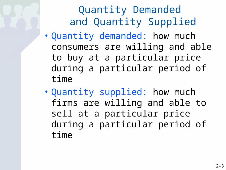
Quantity Demanded and Quantity Supplied

• Quantity demanded: how much consumers are willing and able to buy at a particular price during a particular period of time

• Quantity supplied: how much firms are willing and able to sell at a particular price during a particular period of time

2-4

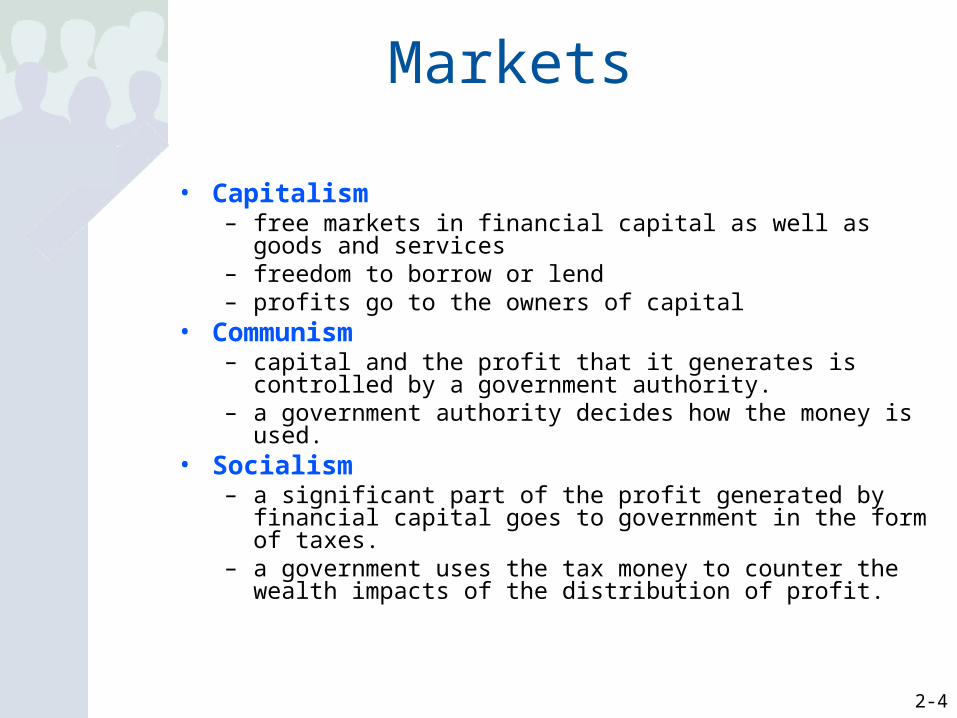
Markets

• Capitalism – free markets in financial capital as well as goods and services– freedom to borrow or lend– profits go to the owners of capital

• Communism– capital and the profit that it generates is controlled by a

government authority. – a government authority decides how the money is used.

• Socialism– a significant part of the profit generated by financial capital goes

to government in the form of taxes. – a government uses the tax money to counter the wealth impacts

of the distribution of profit.

 Hong Kong 1   [90.3]

 Singapore 2   [87.4]

 Ireland 3   [82.4]

 Australia 4   [82.0]

 United States 5   [80.6]

 New Zealand 6   [80.2]

 Canada 7   [80.2]

 Chile 8   [79.8]

 Switzerland 9   [79.7]

 United Kingdom 10   [79.5]

 Denmark 11   [79.2]

 Estonia 12   [77.8]

 Netherlands 13   [76.8]

 Iceland 14   [76.5]

 Luxembourg 15   [75.2]

 Finland 16   [74.8]

 Japan 17   [72.5]

 Mauritius 18   [72.3]

 Bahrain 19   [72.2]

 Belgium 20   [71.5]

Heritage Foundation Index of Economic Freedom (Most Free)

Heritage Foundation Index of Economic Freedom (Most Oppressed)

 Haiti 138   [48.9]

 Sierra Leone 139   [48.9]

 Togo 140   [48.8]

 Central African Republic 141   [48.2]

 Chad 142   [47.7]

 Angola 143   [47.1]

 Syria 144   [46.6]

 Burundi 145   [46.3]

 Congo, Republic of 146   [45.2]

 Guinea Bissau 147   [45.1]

 Venezuela 148   [45.0]

 Bangladesh 149   [44.9]

 Belarus 150   [44.7]

 Iran 151   [44.0]

 Turkmenistan 152   [43.4]

 Burma 153   [39.5]

 Libya 154   [38.7]

 Zimbabwe 155   [29.8]

 Cuba 156   [27.5]

 Korea, North 157   [3.0]

2-7

The Scientific Method and Ceteris Paribus

• Scientists – conduct experiments in laboratories.– use replication and verification to ensure the accuracy of

their conclusions.• Social Scientists

– cannot experiment on their subjects.– must use models and look at the effects of individual

variables within those models.• Economists

– hold variables constant within models to examine the effect of other variables.

– use the Latin phrase ceteris paribus which means “holding other things equal” to identify this is the case.

2-8

Demand and Supply

• Demand is the relationship between price and quantity demanded, ceteris paribus.

• Supply is the relationship between price and quantity supplied, ceteris paribus.

2-9

The Supply and Demand Model

2-10

The Demand Schedule• The Demand Schedule presents, in tabular

form, the price and quantity demanded for a good.

Price Individual QD QD for 10,000

$0.00 5 50,000

$0.50 4 40,000

$1.00 3 30,000

$1.50 2 20,000

$2.00 1 10,000

$2.50 0 0

2-11

Figure 1 The Demand Curve

0 10 20 30 40 50

P

Q/t

$2.50

$2.00

$1.50

$1.00

$0.50

0

Demand

2-12

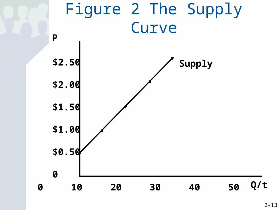
The Supply Schedule• The Supply Schedule presents, in tabular

form, the price and quantity supplied for a good.

Price Individual Qs QS for 10 firms

$0.00 0 0

$0.50 0 0

$1.00 1,000 10,000

$1.50 2,000 20,000

$2.00 3,000 30,000

$2.50 4,000 40,000

2-13

Figure 2 The Supply Curve

0 10 20 30 40 50

P

Q/t

$2.50

$2.00

$1.50

$1.00

$0.50

0

Supply

2-14

Equilibrium, Shortages, and Surpluses

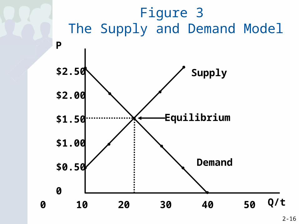
• Equilibrium is the point where the amount that consumers want to buy and the amount that firms want to sell are the same. This occurs where the supply curve and the demand curve cross.

• Shortage (Excess Demand): the condition where firms do not want to sell as many as consumers want to buy.

• Surplus (Excess Supply): the condition where firms want to sell more than consumers want to buy

2-15

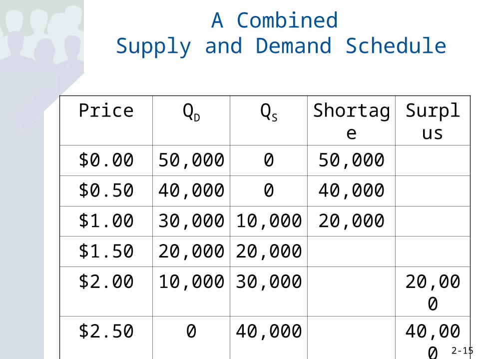
A Combined Supply and Demand Schedule

Price QD QS Shortage Surplus

$0.00 50,000 0 50,000

$0.50 40,000 0 40,000

$1.00 30,000 10,000 20,000

$1.50 20,000 20,000

$2.00 10,000 30,000 20,000

$2.50 0 40,000 40,000

2-16

Figure 3 The Supply and Demand Model

0 10 20 30 40 50

P

Q/t

$2.50

$2.00

$1.50

$1.00

$0.50

0

Supply

Demand

Equilibrium

2-17

All About Demand

• The Law of Demand– The relationship between price and quantity

demanded is a negative or inverse one.

2-18

Why Does the Law of Demand Make Sense?

• The Substitution Effect– moves people toward the good that is now cheaper

or away from the good that is now more expensive

• The Real Balances Effect– When a price increases it decreases your buying

power causing you to buy less.

• The Law of Diminishing Marginal Utility– The amount of additional happiness that you get

from an additional unit of consumption falls with each additional unit.

2-19

The Law of Supply

• The Law of Supply is the statement that there is a positive relationship between price and quantity supplied.

2-20

Why Does the Law of Supply Make Sense?

• Because of Increasing Marginal Costs firms require higher prices to produce more output.

2-21

Determinants of Demand

• Taste• Income

– Normal Goods– Inferior Goods

• Price of Other Goods– Complement– Substitute

• Population of Potential Buyers• Expected Price

2-22

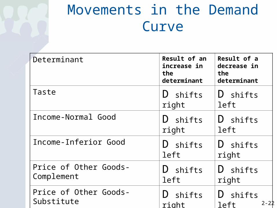
Movements in the Demand Curve

Determinant Result of an increase in the determinant

Result of a decrease in the determinant

Taste D shifts right D shifts left

Income-Normal Good D shifts right D shifts left

Income-Inferior Good D shifts left D shifts right

Price of Other Goods-Complement D shifts left D shifts right

Price of Other Goods-Substitute D shifts right D shifts left

Population of Potential Buyers D shifts right D shifts left

Expected Future Price D shifts right D shifts left

2-23

Figure 4 The Effect of an Increase in Demand

New Demand

New Equilibrium

0 10 20 30 40 50

P

Q/t

$2.50

$2.00

$1.50

$1.00

$0.50

0

Demand

Supply

Old Equilibrium

2-24

Figure 5 The Effect of a Decrease in Demand

0 10 20 30 40 50

P

Q/t

$2.50

$2.00

$1.50

$1.00

$0.50

0Demand

Supply

Old Equilibrium

New Demand

New Equilibrium

2-25

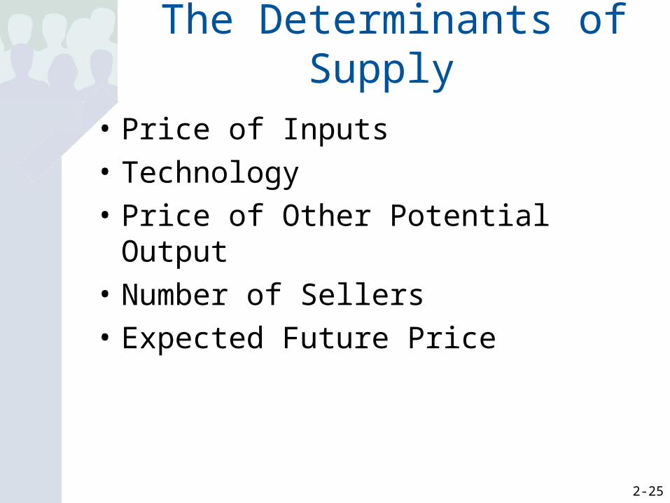
The Determinants of Supply

• Price of Inputs

• Technology

• Price of Other Potential Output

• Number of Sellers

• Expected Future Price

2-26

Movements in the Supply Curve

Determinant Result of an increase in the determinant

Result of a decrease in the determinant

Price of Inputs S shifts left S shifts right

Technology S shifts right S shifts left

Price of Other Potential Outputs

S shifts left S shifts right

Number of Sellers S shifts right S shifts left

Expected Future Price S shifts left S shifts right

2-27

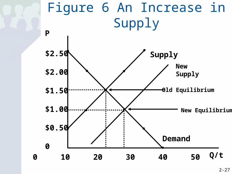
Figure 6 An Increase in Supply

0 10 20 30 40 50

P

Q/t

$2.50

$2.00

$1.50

$1.00

$0.50

0Demand

Supply

Old Equilibrium

New Equilibrium

New Supply

2-28

Figure 7 A Decrease in Supply

0 10 20 30 40 50

P

Q/t

$2.50

$2.00

$1.50

$1.00

$0.50

0Demand

Supply

Old Equilibrium

New SupplyNew

Equilibrium

2-29

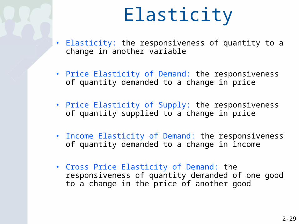
Elasticity• Elasticity: the responsiveness of quantity to a change in

another variable

• Price Elasticity of Demand: the responsiveness of quantity demanded to a change in price

• Price Elasticity of Supply: the responsiveness of quantity supplied to a change in price

• Income Elasticity of Demand: the responsiveness of quantity demanded to a change in income

• Cross Price Elasticity of Demand: the responsiveness of quantity demanded of one good to a change in the price of another good

2-30

The Mathematical Representation of Elasticity

Elasticity =%ΔQ

%ΔP=

ΔQ

ΔP

Q

P

Because the demand curve is downward sloping and the supply curve is upward sloping the elasticity of demand is negative and the elasticity of supply is positive. Often these signs are implicit and ignored.

2-31

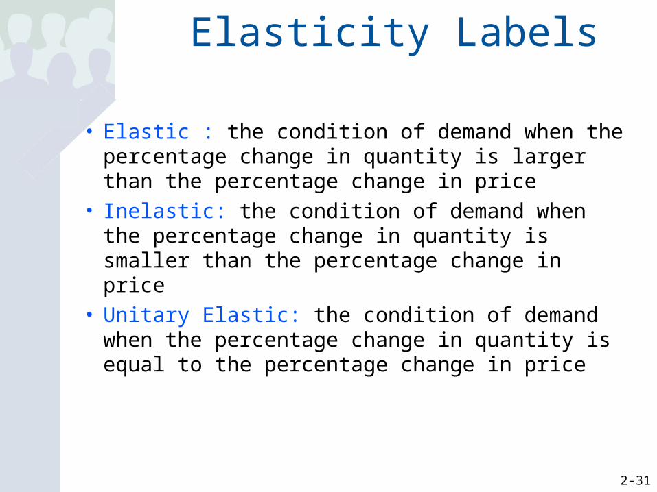
Elasticity Labels

• Elastic : the condition of demand when the percentage change in quantity is larger than the percentage change in price

• Inelastic: the condition of demand when the percentage change in quantity is smaller than the percentage change in price

• Unitary Elastic: the condition of demand when the percentage change in quantity is equal to the percentage change in price

2-32

Alternative Ways to Understand Elasticity

The Graphical Explanation

2-33

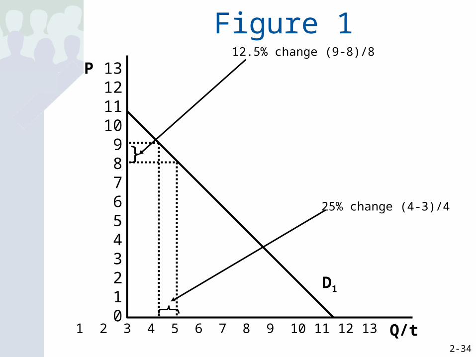
The Relationship Between Slope and Elasticity

• Elasticity and the slope of the demand curve are not the same but they are related.

• At a given price level, elasticity is greater with a flatter demand curve.

• With a linear demand curve (meaning a demand curve that has a single value for the slope) elasticity is greater at higher prices

2-34

Figure 1

D1

Q/t

P 13121110

9876543210

1 2 3 4 5 6 7 8 9 10 11 12 13

12.5% change (9-8)/8

25% change (4-3)/4

2-35

Figure 2

D2

Q/t

P 13121110

9876543210

1 2 3 4 5 6 7 8 9 10 11 12 13

50% change (12-8)/8

25% change (4-3)/4

2-36

Figure 3 Higher Prices Means Greater Elasticity

Demand

Q/t

P 13121110

9876543210

1 2 3 4 5 6 7 8 9 10 11 12 13

B

A

CD

12.5% change (9-8)/8

25% change (4-3)/4

50% change (3-2)/2

9.1% change (11-10)/11

2-37

Alternative Ways to Understand Elasticity

• A good for which there are no good substitutes is likely to be one for which you must pay whatever price is charged. It is also likely to be one for which a lower price will not induce substantially greater consumption. Thus, as price changes there is very little change in consumption, i.e. demand is inelastic and the demand curve is steep.

• Inexpensive goods that take up little of your income can change in price and your consumption will not change dramatically. Thus, at low prices, demand is inelastic.

The Verbal Explanation

2-38

Seeing Elasticity Through Total Expenditures

• Total Expenditure Rule: if the price and the amount you spend both go in the same direction then demand is inelastic while if they go in opposite directions demand is elastic.

2-39

Determinants of Elasticity

• Number of and Closeness of Substitutes– The more alternatives you have the less

likely you are to pay high prices for a good and the more likely you are to settle for something that will do.

• Time– The longer you have to come up with

alternatives to paying high prices the more likely it is you will shift to those alternatives.

2-40

Extremes of Elasticity

• Perfectly Inelastic: the condition of demand when price changes have no effect on quantity

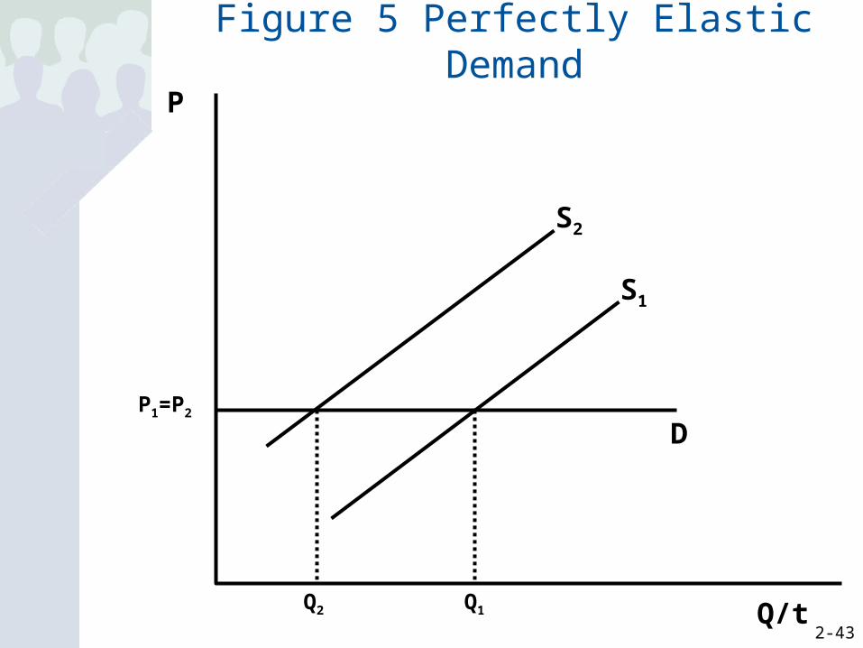
• Perfectly Elastic: the condition of demand when price cannot change

2-41

Elasticity and the Demand Curve

How the Elasticity of Demand Affects Reactions to Price

Changes

2-42

Figure 4 Perfectly Inelastic Demand

D

Q/t

P

S2

Q1=Q2

P2 S1

P1

2-43

Figure 5 Perfectly Elastic Demand

Q/t

P

D

S2

P1=P2

Q2

S1

Q1

2-44

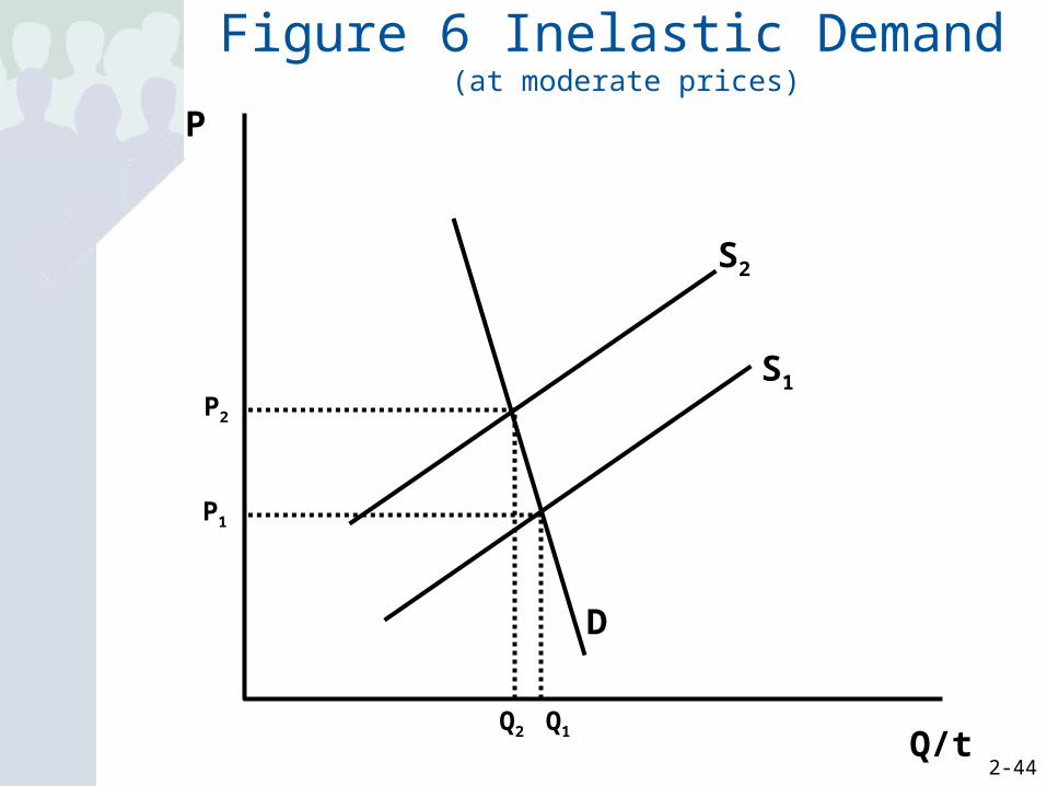
Figure 6 Inelastic Demand (at moderate prices)

P

Q/t

D

S1

P1

Q1Q2

S2

P2

2-45

Figure 7 Elastic Demand(at moderate prices)

Q/t

P

Q1

D

S1

P1

S2

P2

Q2

2-46

Elasticity ExamplesInelastic Goods Price Elasticity

Eggs 0.06

Food 0.21

Health Care Services 0.18

Gasoline (short-run) 0.08

Gasoline (long-run) 0.24

Highway and Bridge Tolls 0.10

Unit Elastic Good (or close to it)

Shellfish 0.89

Cars 1.14

Elastic Goods

Luxury Car 3.70

Foreign Air Travel 1.77

Restaurant Meals 2.27

2-47

Price Elasticity Supply

• Identical in concept to elasticity of demand.– Formula is the Same– It is also related to the slope of the supply

curve but is not simply the slope of the supply curve.

– Terminology is the same

2-48

S

Q/t

P

D2

Q1=Q2

P2

D1

P1

Perfectly Inelastic Supply

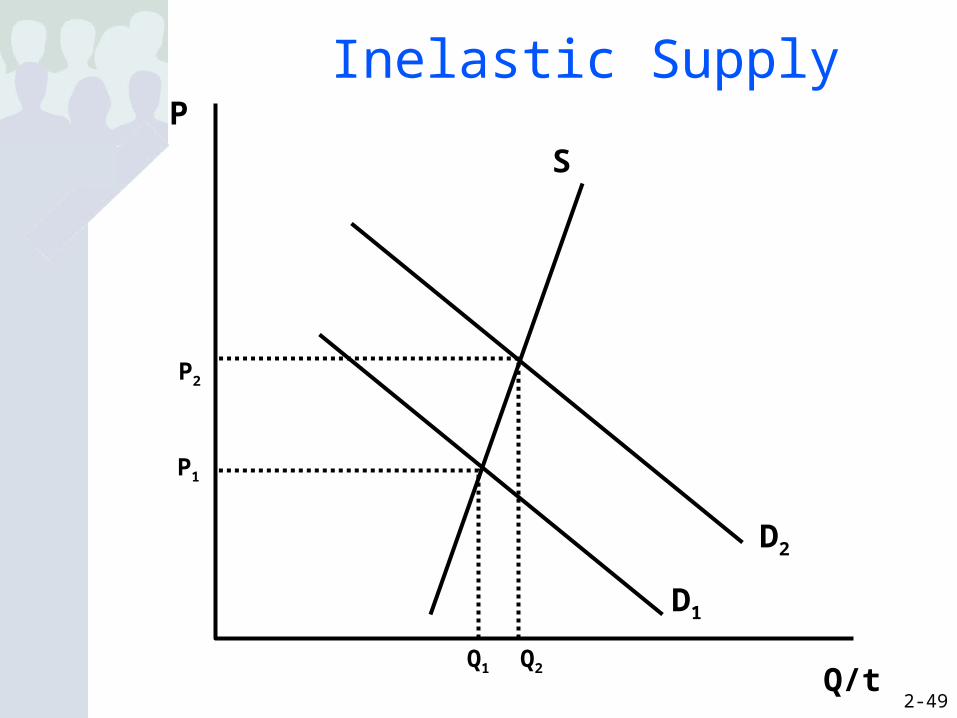
2-49

P

Q/t

P1

Q1 Q2

P2

S

D2

D1

Inelastic Supply

2-50Q/t

P

Q1

P1

P2

Q2

S

D2

D1

Elastic Supply

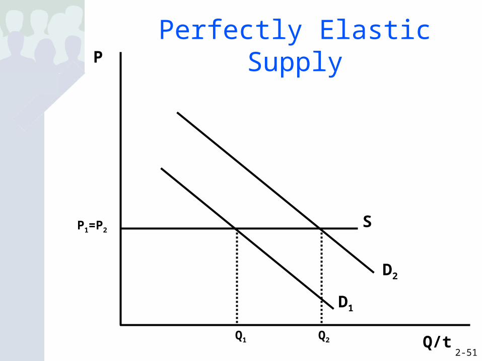
2-51Q/t

P

P1=P2

Q2Q1

S

D2

D1

Perfectly Elastic Supply

2-52

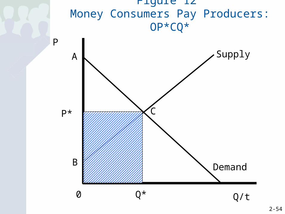
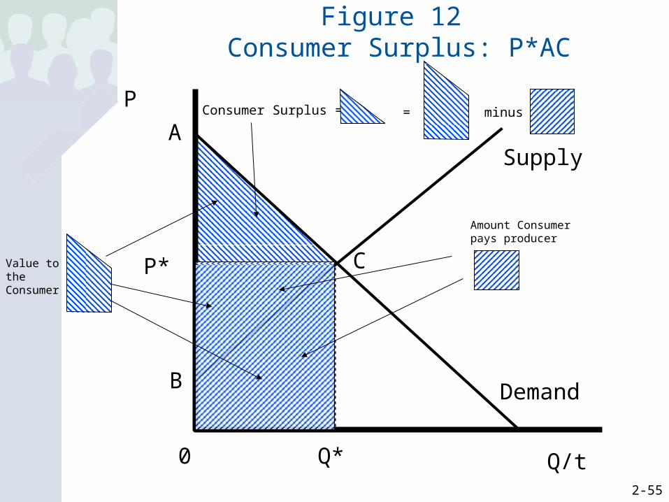
Consumer and Producer Surplus

• Consumer Surplus: the value you get that is in excess of what you pay to get it – On a graph, consumer surplus is the area

below the demand curve and above the price line.

• Producer Surplus: the money the firm gets that is in excess of its marginal costs– On a graph, producer surplus is the area

below the price line and above the supply curve.

2-53

Figure 12 Value to the Consumer: OACQ*

Q/t

P

0

Supply

Demand

P*

Q*

A

B

C

2-54

Figure 12 Money Consumers Pay Producers: OP*CQ*

P

Q/t0

Supply

Demand

P*

Q*

A

B

C

2-55

Figure 12 Consumer Surplus: P*AC

C

P

Q/t0

Supply

Demand

P*

Q*

A

B

Value tothe Consumer

Amount Consumerpays producer

Consumer Surplus = minus=

2-56

Figure 13 Variable Cost to the Producer: OBCQ*

P

0

Supply

Demand

P*

Q*

A

B

C

2-57

P

Q/t0

Supply

Demand

P*

Q*

A

B

C

Amount consumerpays producer

Variable cost toproducer

Producer Surplus = minus=

Figure 13 Producer Surplus: BP*C

2-58

P

Q/t0

Supply

Demand

P*

Q*

A

B

C

ConsumerSurplus

ProducerSurplus

Figure 14 Net Benefit to Society = CS+PS: BAC

2-59

Market Failure• Market Failure: the circumstance where the

market outcome is not the economically efficient outcome– Possible Sources:

• Consumption or production can harm an innocent third party.

• A good may not be one for which a company can profit from selling it though society profits from its existence.

• The buyer may not be able to make a well-informed choice.

• A buyer or seller may have too much power over the price.

2-60

Exclusivity and Rivalry• Exclusivity: the degree to which the

consumption of the good can be restricted by a seller to only those who pay for it

• Rivalry: the degree to which one person’s consumption reduces the value of the good for the next consumer

2-61

Private and Public Goods

• Purely private good: a good with the characteristics of both exclusivity and rivalry

• Purely public good: a good with the neither of the characteristics exclusivity and rivalry

• Excludable public good: a good with the characteristic of exclusivity but not of rivalry

• Congestible public good: a good with the characteristic of rivalry but not of exclusivity

2-62

Kick it Up a Notch

Consumer and Producer Surplus in a Supply and

Demand Model

2-63

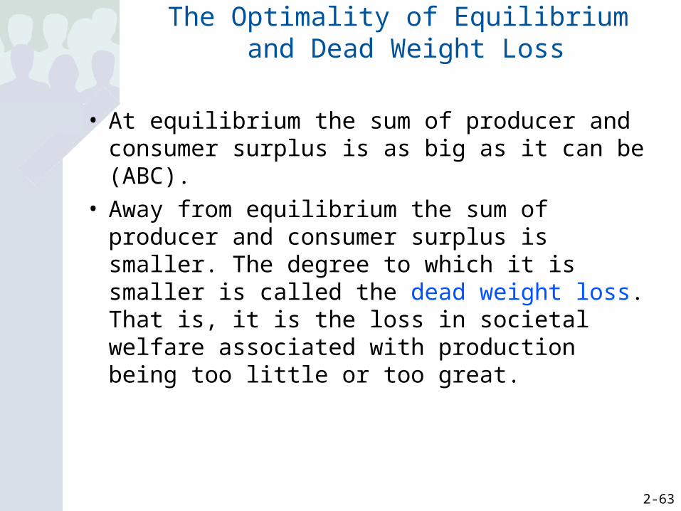
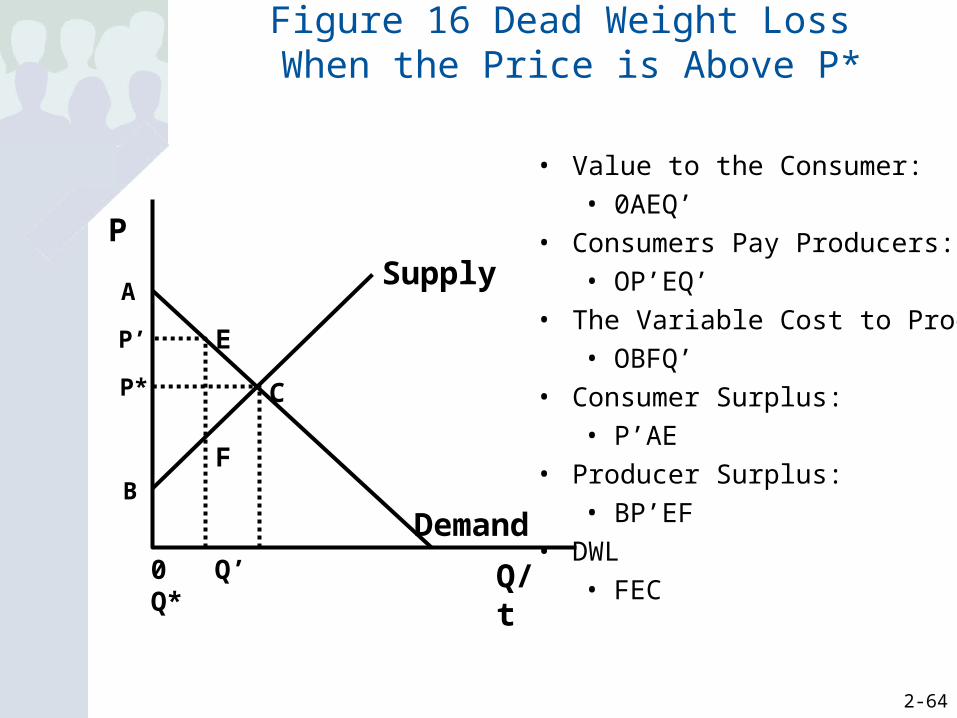
The Optimality of Equilibrium and Dead Weight Loss

• At equilibrium the sum of producer and consumer surplus is as big as it can be (ABC).

• Away from equilibrium the sum of producer and consumer surplus is smaller. The degree to which it is smaller is called the dead weight loss. That is, it is the loss in societal welfare associated with production being too little or too great.

2-64

Figure 16 Dead Weight Loss When the Price is Above P*

Q/t

P

Demand

SupplyA

C

0 Q’ Q*

E

F

P’

P*

B

• Value to the Consumer: • 0AEQ’

• Consumers Pay Producers: • OP’EQ’

• The Variable Cost to Producers: • OBFQ’

• Consumer Surplus: • P’AE

• Producer Surplus: • BP’EF

• DWL• FEC

2-65

Figure 17 Dead Weight Loss When the Price is Below P*

Q/t

P

Demand

SupplyA

P* C

0 Q’ Q*

E

FP’

B

• Value to the Consumer: • 0AEQ’

• Consumers Pay Producers: • OP’FQ’

• The Variable Cost to

Producers: • OBFQ’

• Consumer Surplus: • P’AEF

• Producer Surplus: • BP’F

• DWL• FEC

2-66

Basic Definitions

• Profit: The money that business makes: Revenue minus Cost

• Cost: the expense that must be incurred in order to produce goods for sale

• Revenue : the money that comes into the firm from the sale of their goods

2-67

Economic vs. Accounting Cost

• Economic Cost: All costs, both those that must be paid as well as those incurred in the form of forgone opportunities, of a business

• Accounting Cost: Only those costs that must be explicitly paid by the owner of a business

2-68

Production

• Production Function: a graph which shows how many resources we need to produce various amounts of output

• Cost Function: a graph which shows how much various amounts of production cost

2-69

Inputs to Production

• Fixed Inputs: resources that you cannot change

• Variable Inputs : resources that can be easily changed

2-70

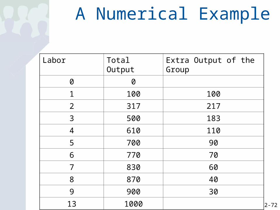
Concepts in Production

• Division of Labor: workers divide up the tasks in such a way that each can build up a momentum and not have to switch jobs

• Diminishing Returns: the notion that there exists a point where the addition of resources increases production but does so at a decreasing rate

2-71

Figure 1 The Production Function

Output

Workers

Production Function

AB

C

D

2-72

A Numerical Example

Labor Total Output Extra Output of the Group

0 0

1 100 100

2 317 217

3 500 183

4 610 110

5 700 90

6 770 70

7 830 60

8 870 40

9 900 30

13 1000

2-73

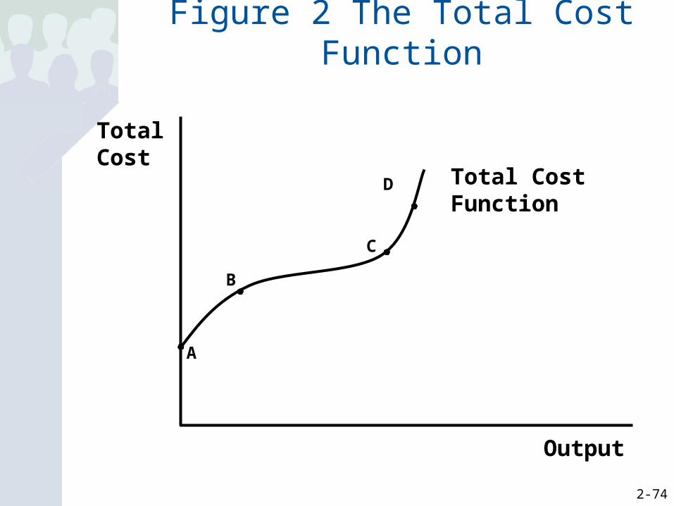
Costs

• Fixed Costs: costs of production that we cannot change

• Variable Costs: costs of production that we can change

2-74

Figure 2 The Total Cost Function

Output

Total Cost

Total Cost Function

A

B

C

D

2-75

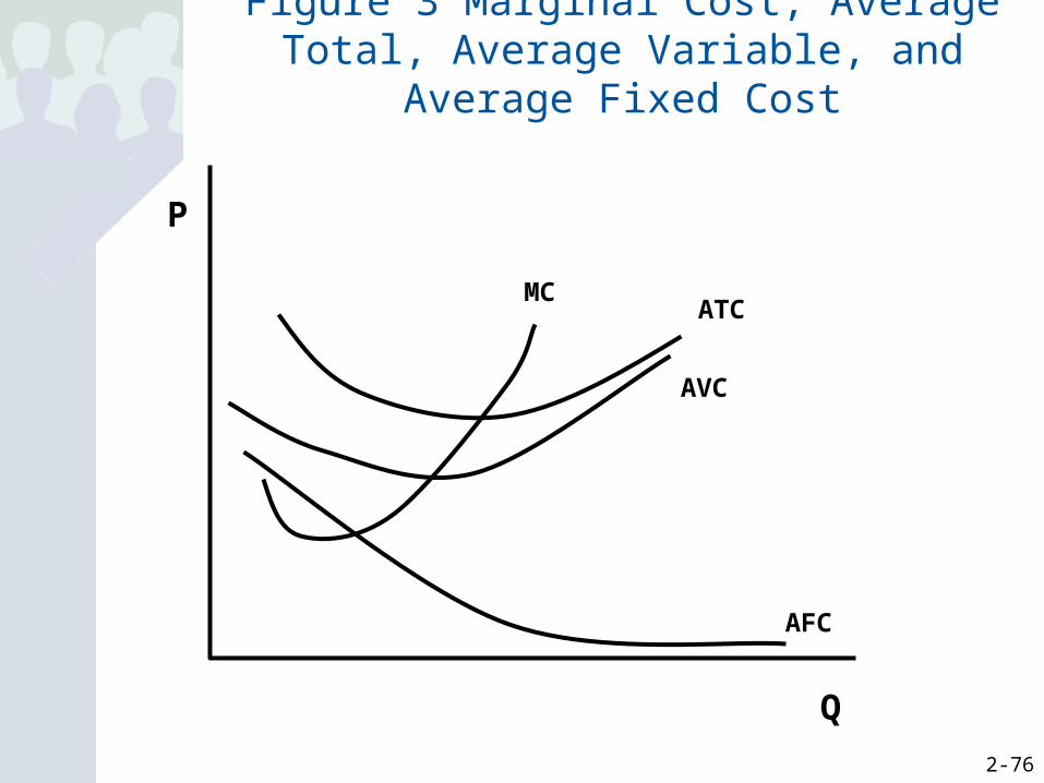
Cost Concepts

• Marginal Cost: the addition to cost associated with one additional unit of output

• Average Total Cost: Total Cost/Output, the cost per unit of production

• Average Variable Cost: Total Variable Cost/Output, the average variable cost per unit of production

• Average Fixed Cost: Total Fixed Cost/Output, the average fixed cost per unit of production

2-76

Figure 3 Marginal Cost, Average Total, Average Variable, and Average Fixed Cost

P

Q

MCATC

AVC

AFC

2-77

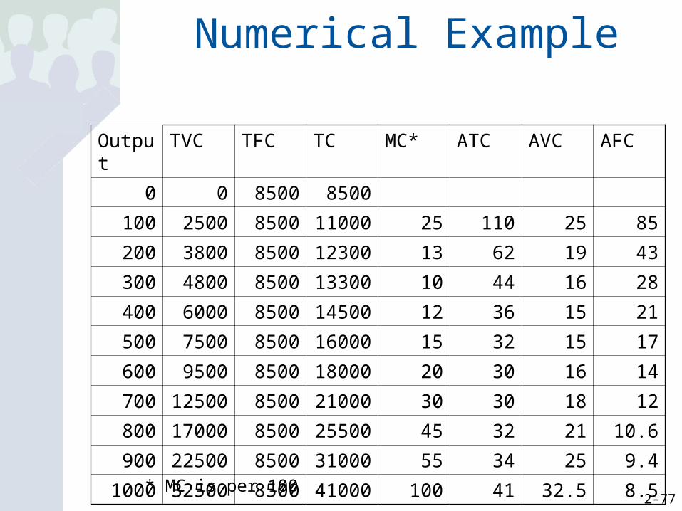
Numerical Example

Output TVC TFC TC MC* ATC AVC AFC

0 0 8500 8500

100 2500 8500 11000 25 110 25 85

200 3800 8500 12300 13 62 19 43

300 4800 8500 13300 10 44 16 28

400 6000 8500 14500 12 36 15 21

500 7500 8500 16000 15 32 15 17

600 9500 8500 18000 20 30 16 14

700 12500 8500 21000 30 30 18 12

800 17000 8500 25500 45 32 21 10.6

900 22500 8500 31000 55 34 25 9.4

1000 32500 8500 41000 100 41 32.5 8.5* MC is per 100

2-78

Revenue

• Marginal Revenue : additional revenue the firm receives from the sale of each unit

2-79

Figure 4 Setting the Price When There are Many Competitors

Our Firm

P

Market for Memory

P

D

S

P*P*=Marginal Revenue

2-80

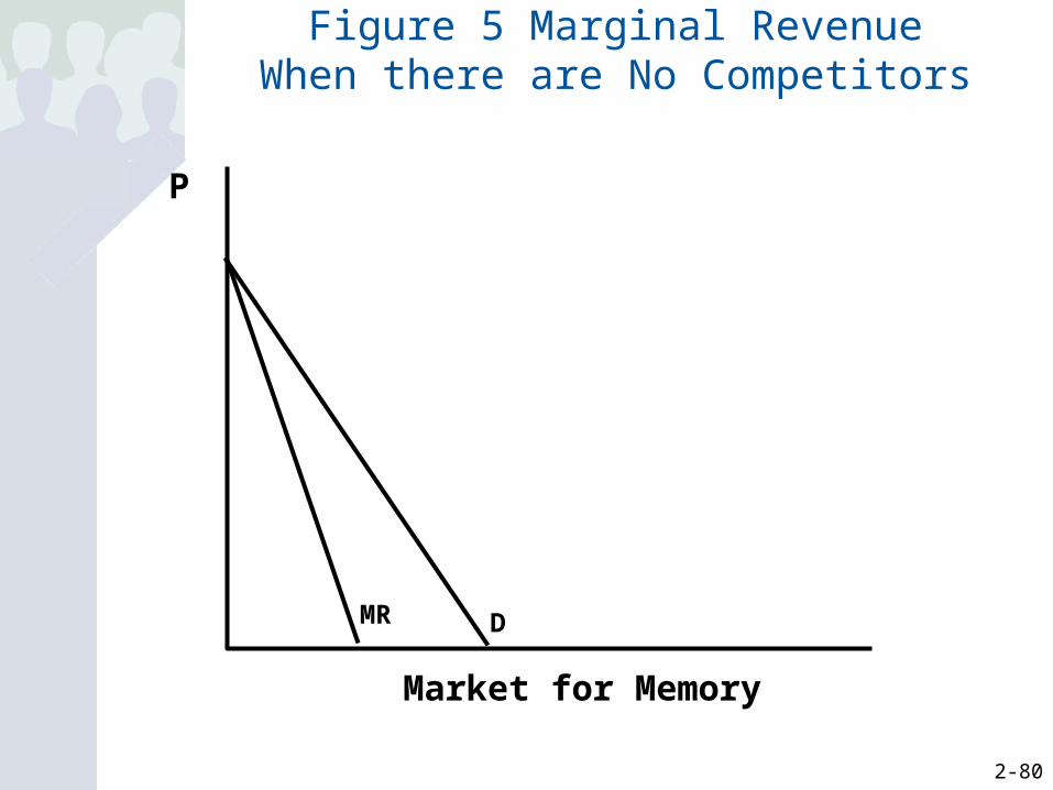
Figure 5 Marginal Revenue When there are No Competitors

MR

Market for Memory

P

D

2-81

Numerical Example For the Many Competitors Case

Q P TR MR*

0 45 0

100 45 4,500 45

200 45 9,000 45

300 45 13,500 45

400 45 18,000 45

500 45 22,500 45

600 45 27,000 45

700 45 31,500 45

800 45 36,000 45

900 45 40,500 45

1000 45 45,000 45* MR is per 100

2-82

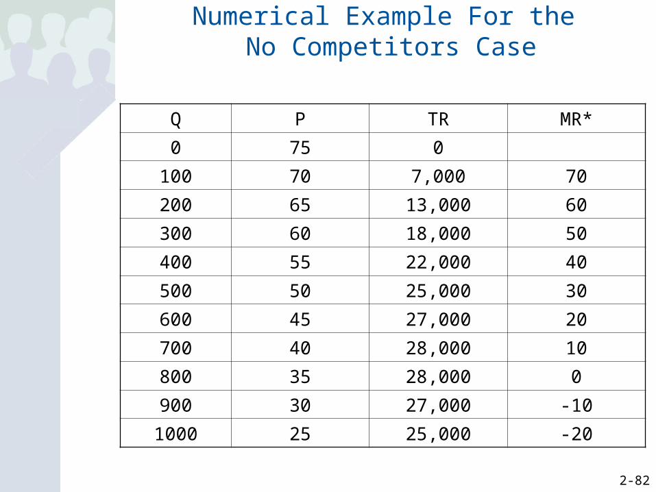
Numerical Example For the No Competitors Case

Q P TR MR*

0 75 0

100 70 7,000 70

200 65 13,000 60

300 60 18,000 50

400 55 22,000 40

500 50 25,000 30

600 45 27,000 20

700 40 28,000 10

800 35 28,000 0

900 30 27,000 -10

1000 25 25,000 -20

2-83

Maximizing Profit

• We assume that firms wish to maximize profits

2-84

Market Forms

• Perfect Competition: a situation in a market where there are many firms producing the same good

• Monopoly: a situation in a market where there is only one firm producing the good

2-85

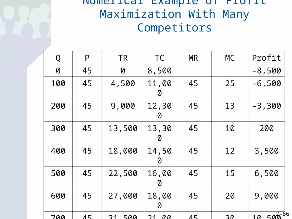
Rules of Production

• A firm should a) produce an amount such that Marginal

Revenue equals Marginal Cost (MR=MC),

unless

b) the price is less than the average variable cost (P<AVC).

2-86

Numerical Example of Profit Maximization With Many Competitors

Q P TR TC MR MC Profit

0 45 0 8,500 -8,500

100 45 4,500 11,000 45 25 -6,500

200 45 9,000 12,300 45 13 -3,300

300 45 13,500 13,300 45 10 200

400 45 18,000 14,500 45 12 3,500

500 45 22,500 16,000 45 15 6,500

600 45 27,000 18,000 45 20 9,000

700 45 31,500 21,000 45 30 10,500

800 45 36,000 25,500 45 45 10,500

900 45 40,500 31,000 45 55 9,500

1000 45 45,000 41,000 45 75 4,000

2-87

Numerical Example of Profit Maximization With No Competitors

Q P TR TC MR MC Profit

0 75 0 8,500 -8,500

100 70 7,000 11,000 70 25 -6,500

200 65 13,000 12,300 60 13 -3,300

300 60 18,000 13,300 50 10 200

400 55 22,000 14,500 40 12 3,500

500 50 25,000 16,000 30 15 6,500

600 45 27,000 18,000 20 20 9,000

700 40 28,000 21,000 10 30 7,000

800 35 28,000 25,500 0 45 2,500

900 30 27,000 31,000 -10 55 -4,000

1000 25 25,000 41,000 -20 75 -16,000