Technical report

Neutron Transmission StrainTomography for Non-ConstantStress-Free Lattice Spacing

J.N. Hendriks, C. Jidling, T.B. Schon, A. Wills, C.M. Wensrich, E.H. Kisi

• Please cite this version:

J.N. Hendriks, C. Jidling, T.B. Schon, A. Wills, C.M. Wensrich, E.H. Kisi. NeutronTransmission Strain Tomography for Non-Constant Stress-Free Lattice Spacing. Nuclearinstruments and methods in physics research section B, 456:64-73, 2019.

arX

iv:1

905.

0685

4v2

[ph

ysic

s.co

mp-

ph]

18

Jul 2

019

Neutron Transmission Strain Tomography for Non-Constant

Stress-Free Lattice Spacing

J.N. Hendriks1, C. Jidling2, T.B. Schon2, A. Wills1, C.M. Wensrich1, and E.H. Kisi1

1School of Engineering, The University of Newcastle, Callaghan NSW 2308, Australia2Department of Information Technology, Uppsala University, Sweden

July 19, 2019

Abstract

Recently, several algorithms for strain tomography from energy-resolved neutron transmission mea-surements have been proposed. These methods assume that the stress-free lattice spacing d0 is a knownconstant limiting their application to the study of stresses generated by manufacturing and loading meth-ods that do not alter this parameter. In this paper, we consider the more general problem of jointlyreconstructing the strain and d0 fields. A method for solving this inherently non-linear problem is pre-sented that ensures the estimated strain field satisfies equilibrium and can include knowledge of boundaryconditions. This method is tested on a simulated data set with realistic noise levels, demonstrating thatit is possible to jointly reconstruct d0 and the strain field.

1 Introduction

Energy-resolved neutron transmission methods can generate lower dimensional (one- or two-dimensional)images of strain from a higher dimensional (two- or three-dimensional) strain field within a polycrystallinematerial. The ‘tomographic’ reconstruction of an unknown strain field from these images can be used to studythe residual strain and stress within engineering components. Residual stresses are those which remain afterapplied loads are removed (e.g. due to heat treatment, plastic deformation, etc.), and may have significantand unintended impact on a component’s effective strength and service life — in particular its fatigue life.Measuring and quantifying these strains is important for the validation of predictive design tools, such asFinite Element Analysis, and to aid the development of novel manufacturing techniques — i.e. additivemanufacturing.

These strain images are generated by analysing features known as Bragg-edges in the relative transmission of aneutron pulse through a sample. Bragg-edges are sudden increases in the intensity as a function of wavelengthand occur when the scattering angle 2ϑ reaches 180◦, beyond which no further coherent scattering can occur.The wavelength λ at which these Bragg-edges occur can be related to the lattice spacing d within the samplethrough Bragg’s law: λ = 2d sinϑ. Assuming minimal texture, this can be used to provide a relative measureof strain;

〈ε〉 =d− d0d0

, (1)

where d0 is the stress-free lattice spacing and 〈ε〉 is a through thickness average of the normal, elastic strainin the direction of the beam.

The determination of d0 is a problem inherent to diffraction and transmission strain analysis. For specificcases where the loading mechanism does not result in changes to the stress-free lattice parameter, its valuecan be measured prior to loading and in the simplest case (e.g. for an annealed sample) a constant valuethroughout the sample can be assumed. Several algorithms for strain tomography assuming a known, constantstress-free lattice spacing have been developed. Reconstruction of axisymmetric strain fields is considered in

1

(Abbey et al., 2009, 2012; Kirkwood et al., 2015; Gregg et al., 2017) and more general two-dimensional strainfields in (Gregg et al., 2018; Jidling et al., 2018; Hendriks et al., 2018a).

Many manufacturing techniques (e.g. welding and additive manufacturing) can alter the lattice spacing; forexample, as a result of inhomogeneously distributed phase changes (such as the Martensite transformation),or due to gradients in composition as a result of differing chemical states in the starting materials. Sincethe lattice spacing (in this case d0) is sensitive to crystal structure and composition changes, the stress-freelattice parameter may vary throughout the sample. Ignoring variations in d0 would cause severe degradationin the quality of a reconstructed strain field. In such cases, measuring d0 is more challenging and has beenachieved in neutron diffraction measurements by measuring additional directions of strain (Luzin et al., 2011;Choi et al., 2007) and by destructive methods where the strain is relieved by wire cutting the sample into agrid allowing the stress-free lattice spacing to be measured throughout the sample (Paradowska et al., 2005).Although the latter of these two options could be applied to strain tomography it requires the destructionof the sample and creates an additional tomography problem, requiring another set of measurements to beacquired.

Here, we present a method capable of jointly reconstructing the strain field and the d0 field from a single setof neutron transmission images. To achieve this both the strain and d0 are modelled by a Gaussian process(see for example Rasmussen and Williams (2006)) and equilibrium and boundary conditions are built into thestrain model (Jidling et al., 2017). This extends the Gaussian process approach presented by Jidling et al.(2018); Hendriks et al. (2018a) to handle the inherently non-linear nature of this problem. A numericallytractable algorithm based on variational inference (see for example Blei et al. (2017); Jordan et al. (1999)) isprovided and the method is validated on a simulated data set.

2 Problem Statement

This paper focuses on the joint reconstruction of the strain field ε(x) and a non-constant stress-free latticeparameter d0(x) from a set of neutron transmission images. Restricting the problem to two dimensions, givesthe strain field as the symmetric tensor

ε(x) =

[εxx(x) εxy(x)εxy(x) εyy(x)

], (2)

where x =[x y

]T. For brevity, the unique components of strain will be written as ε =

[εxx εxy εyy

]Twith the coordinate x omitted where appropriate.

Here, we consider the lattice spacings d as the measurements rather than the standard approach whichconsiders the relative strain of the form form (1). This allows the measurements to be explicitly relatedto both the strain and the stress-free lattice parameter through the Longitudinal Ray Transform (LRT)(Lionheart and Withers, 2015):

y(η) = d(η) + e =1

L

L∫0

nε(p + ns)d0(p + ns) + d0(p + ns) ds+ e. (3)

where e ∼ N (0, σ2n) and the geometry of each measurement is given by the parameter set η = {n, L,p};

with n as the beam direction, L as the irradiation length, p =[x0 y0

]Tas the point of initial intersection

between the ray and the sample, and n =[n21 2n1n2 n22

]. See Figure 1 for the measurement geometry.

These measurements are a non-linear function of the two phenomena we wish to estimate; ε and d0.

For details on the analysis of neutron transmission data to determine these lattice spacings the reader isreferred to Santisteban et al. (2002b,a); Tremsin et al. (2011, 2012). It is also worth noting that the standarddeviation σn of these measurements is available.

Furthermore, the strain field inside a sample is a physical property and as such it is subject to equilibriumand boundary conditions (Sadd, 2009). Therefore, it is natural to constrain estimates of the strain field to

2

L

✏(x)

n, s<latexit sha1_base64="T0p+LpjylXATewHWonNd5WuWcZs=">AAAB/3icbVBPS8MwHP11/pvzX1Xw4iU4BA8yWhH0OPTicYKbg7WMNM22sDQtSSqM2oNfxYsHRbz6Nbz5bUy3HnTzQcjjvd+PvLwg4Uxpx/m2KkvLK6tr1fXaxubW9o69u9dRcSoJbZOYx7IbYEU5E7Stmea0m0iKo4DT+2B8Xfj3D1QqFos7PUmoH+GhYANGsDZS3z7wRlhnXhDzUE0ic2Uiz09V3647DWcKtEjcktShRKtvf3lhTNKICk04VqrnOon2Myw1I5zmNS9VNMFkjIe0Z6jAEVV+Ns2fo2OjhGgQS3OERlP190aGI1WkM5MR1iM17xXif14v1YNLP2MiSTUVZPbQIOVIx6goA4VMUqL5xBBMJDNZERlhiYk2ldVMCe78lxdJ56zhOg339rzevCrrqMIhHMEJuHABTbiBFrSBwCM8wyu8WU/Wi/VufcxGK1a5sw9/YH3+APQtlrA=</latexit><latexit sha1_base64="T0p+LpjylXATewHWonNd5WuWcZs=">AAAB/3icbVBPS8MwHP11/pvzX1Xw4iU4BA8yWhH0OPTicYKbg7WMNM22sDQtSSqM2oNfxYsHRbz6Nbz5bUy3HnTzQcjjvd+PvLwg4Uxpx/m2KkvLK6tr1fXaxubW9o69u9dRcSoJbZOYx7IbYEU5E7Stmea0m0iKo4DT+2B8Xfj3D1QqFos7PUmoH+GhYANGsDZS3z7wRlhnXhDzUE0ic2Uiz09V3647DWcKtEjcktShRKtvf3lhTNKICk04VqrnOon2Myw1I5zmNS9VNMFkjIe0Z6jAEVV+Ns2fo2OjhGgQS3OERlP190aGI1WkM5MR1iM17xXif14v1YNLP2MiSTUVZPbQIOVIx6goA4VMUqL5xBBMJDNZERlhiYk2ldVMCe78lxdJ56zhOg339rzevCrrqMIhHMEJuHABTbiBFrSBwCM8wyu8WU/Wi/VufcxGK1a5sw9/YH3+APQtlrA=</latexit><latexit sha1_base64="T0p+LpjylXATewHWonNd5WuWcZs=">AAAB/3icbVBPS8MwHP11/pvzX1Xw4iU4BA8yWhH0OPTicYKbg7WMNM22sDQtSSqM2oNfxYsHRbz6Nbz5bUy3HnTzQcjjvd+PvLwg4Uxpx/m2KkvLK6tr1fXaxubW9o69u9dRcSoJbZOYx7IbYEU5E7Stmea0m0iKo4DT+2B8Xfj3D1QqFos7PUmoH+GhYANGsDZS3z7wRlhnXhDzUE0ic2Uiz09V3647DWcKtEjcktShRKtvf3lhTNKICk04VqrnOon2Myw1I5zmNS9VNMFkjIe0Z6jAEVV+Ns2fo2OjhGgQS3OERlP190aGI1WkM5MR1iM17xXif14v1YNLP2MiSTUVZPbQIOVIx6goA4VMUqL5xBBMJDNZERlhiYk2ldVMCe78lxdJ56zhOg339rzevCrrqMIhHMEJuHABTbiBFrSBwCM8wyu8WU/Wi/VufcxGK1a5sw9/YH3+APQtlrA=</latexit><latexit sha1_base64="T0p+LpjylXATewHWonNd5WuWcZs=">AAAB/3icbVBPS8MwHP11/pvzX1Xw4iU4BA8yWhH0OPTicYKbg7WMNM22sDQtSSqM2oNfxYsHRbz6Nbz5bUy3HnTzQcjjvd+PvLwg4Uxpx/m2KkvLK6tr1fXaxubW9o69u9dRcSoJbZOYx7IbYEU5E7Stmea0m0iKo4DT+2B8Xfj3D1QqFos7PUmoH+GhYANGsDZS3z7wRlhnXhDzUE0ic2Uiz09V3647DWcKtEjcktShRKtvf3lhTNKICk04VqrnOon2Myw1I5zmNS9VNMFkjIe0Z6jAEVV+Ns2fo2OjhGgQS3OERlP190aGI1WkM5MR1iM17xXif14v1YNLP2MiSTUVZPbQIOVIx6goA4VMUqL5xBBMJDNZERlhiYk2ldVMCe78lxdJ56zhOg339rzevCrrqMIhHMEJuHABTbiBFrSBwCM8wyu8WU/Wi/VufcxGK1a5sw9/YH3+APQtlrA=</latexit>

y<latexit sha1_base64="l29WxoUb9DEbvmhLG7jHtZ0OU24=">AAAB6HicbVBNS8NAEJ34WetX1aOXxSJ4KokIeix68diC/YA2lM120q7dbMLuRgihv8CLB0W8+pO8+W/ctjlo64OBx3szzMwLEsG1cd1vZ219Y3Nru7RT3t3bPzisHB23dZwqhi0Wi1h1A6pRcIktw43AbqKQRoHATjC5m/mdJ1Sax/LBZAn6ER1JHnJGjZWa2aBSdWvuHGSVeAWpQoHGoPLVH8YsjVAaJqjWPc9NjJ9TZTgTOC33U40JZRM6wp6lkkao/Xx+6JScW2VIwljZkobM1d8TOY20zqLAdkbUjPWyNxP/83qpCW/8nMskNSjZYlGYCmJiMvuaDLlCZkRmCWWK21sJG1NFmbHZlG0I3vLLq6R9WfPcmte8qtZvizhKcApncAEeXEMd7qEBLWCA8Ayv8OY8Oi/Ou/OxaF1zipkT+APn8wfnvYz9</latexit><latexit sha1_base64="l29WxoUb9DEbvmhLG7jHtZ0OU24=">AAAB6HicbVBNS8NAEJ34WetX1aOXxSJ4KokIeix68diC/YA2lM120q7dbMLuRgihv8CLB0W8+pO8+W/ctjlo64OBx3szzMwLEsG1cd1vZ219Y3Nru7RT3t3bPzisHB23dZwqhi0Wi1h1A6pRcIktw43AbqKQRoHATjC5m/mdJ1Sax/LBZAn6ER1JHnJGjZWa2aBSdWvuHGSVeAWpQoHGoPLVH8YsjVAaJqjWPc9NjJ9TZTgTOC33U40JZRM6wp6lkkao/Xx+6JScW2VIwljZkobM1d8TOY20zqLAdkbUjPWyNxP/83qpCW/8nMskNSjZYlGYCmJiMvuaDLlCZkRmCWWK21sJG1NFmbHZlG0I3vLLq6R9WfPcmte8qtZvizhKcApncAEeXEMd7qEBLWCA8Ayv8OY8Oi/Ou/OxaF1zipkT+APn8wfnvYz9</latexit><latexit sha1_base64="l29WxoUb9DEbvmhLG7jHtZ0OU24=">AAAB6HicbVBNS8NAEJ34WetX1aOXxSJ4KokIeix68diC/YA2lM120q7dbMLuRgihv8CLB0W8+pO8+W/ctjlo64OBx3szzMwLEsG1cd1vZ219Y3Nru7RT3t3bPzisHB23dZwqhi0Wi1h1A6pRcIktw43AbqKQRoHATjC5m/mdJ1Sax/LBZAn6ER1JHnJGjZWa2aBSdWvuHGSVeAWpQoHGoPLVH8YsjVAaJqjWPc9NjJ9TZTgTOC33U40JZRM6wp6lkkao/Xx+6JScW2VIwljZkobM1d8TOY20zqLAdkbUjPWyNxP/83qpCW/8nMskNSjZYlGYCmJiMvuaDLlCZkRmCWWK21sJG1NFmbHZlG0I3vLLq6R9WfPcmte8qtZvizhKcApncAEeXEMd7qEBLWCA8Ayv8OY8Oi/Ou/OxaF1zipkT+APn8wfnvYz9</latexit><latexit sha1_base64="l29WxoUb9DEbvmhLG7jHtZ0OU24=">AAAB6HicbVBNS8NAEJ34WetX1aOXxSJ4KokIeix68diC/YA2lM120q7dbMLuRgihv8CLB0W8+pO8+W/ctjlo64OBx3szzMwLEsG1cd1vZ219Y3Nru7RT3t3bPzisHB23dZwqhi0Wi1h1A6pRcIktw43AbqKQRoHATjC5m/mdJ1Sax/LBZAn6ER1JHnJGjZWa2aBSdWvuHGSVeAWpQoHGoPLVH8YsjVAaJqjWPc9NjJ9TZTgTOC33U40JZRM6wp6lkkao/Xx+6JScW2VIwljZkobM1d8TOY20zqLAdkbUjPWyNxP/83qpCW/8nMskNSjZYlGYCmJiMvuaDLlCZkRmCWWK21sJG1NFmbHZlG0I3vLLq6R9WfPcmte8qtZvizhKcApncAEeXEMd7qEBLWCA8Ayv8OY8Oi/Ou/OxaF1zipkT+APn8wfnvYz9</latexit>

p<latexit sha1_base64="d9UYl+MIsz8lH836NZH6Fir/fh0=">AAAB8XicbVDLSsNAFL2pr1pfVZduBovgqiQi6LLoxmUF+8A2lMn0ph06mYSZiVBC/8KNC0Xc+jfu/BsnbRbaemDgcM69zLknSATXxnW/ndLa+sbmVnm7srO7t39QPTxq6zhVDFssFrHqBlSj4BJbhhuB3UQhjQKBnWBym/udJ1Sax/LBTBP0IzqSPOSMGis99iNqxkGYJbNBtebW3TnIKvEKUoMCzUH1qz+MWRqhNExQrXuemxg/o8pwJnBW6acaE8omdIQ9SyWNUPvZPPGMnFllSMJY2ScNmau/NzIaaT2NAjuZJ9TLXi7+5/VSE177GZdJalCyxUdhKoiJSX4+GXKFzIipJZQpbrMSNqaKMmNLqtgSvOWTV0n7ou65de/+sta4Keoowwmcwjl4cAUNuIMmtICBhGd4hTdHOy/Ou/OxGC05xc4x/IHz+QPxEZEU</latexit><latexit sha1_base64="d9UYl+MIsz8lH836NZH6Fir/fh0=">AAAB8XicbVDLSsNAFL2pr1pfVZduBovgqiQi6LLoxmUF+8A2lMn0ph06mYSZiVBC/8KNC0Xc+jfu/BsnbRbaemDgcM69zLknSATXxnW/ndLa+sbmVnm7srO7t39QPTxq6zhVDFssFrHqBlSj4BJbhhuB3UQhjQKBnWBym/udJ1Sax/LBTBP0IzqSPOSMGis99iNqxkGYJbNBtebW3TnIKvEKUoMCzUH1qz+MWRqhNExQrXuemxg/o8pwJnBW6acaE8omdIQ9SyWNUPvZPPGMnFllSMJY2ScNmau/NzIaaT2NAjuZJ9TLXi7+5/VSE177GZdJalCyxUdhKoiJSX4+GXKFzIipJZQpbrMSNqaKMmNLqtgSvOWTV0n7ou65de/+sta4Keoowwmcwjl4cAUNuIMmtICBhGd4hTdHOy/Ou/OxGC05xc4x/IHz+QPxEZEU</latexit><latexit sha1_base64="d9UYl+MIsz8lH836NZH6Fir/fh0=">AAAB8XicbVDLSsNAFL2pr1pfVZduBovgqiQi6LLoxmUF+8A2lMn0ph06mYSZiVBC/8KNC0Xc+jfu/BsnbRbaemDgcM69zLknSATXxnW/ndLa+sbmVnm7srO7t39QPTxq6zhVDFssFrHqBlSj4BJbhhuB3UQhjQKBnWBym/udJ1Sax/LBTBP0IzqSPOSMGis99iNqxkGYJbNBtebW3TnIKvEKUoMCzUH1qz+MWRqhNExQrXuemxg/o8pwJnBW6acaE8omdIQ9SyWNUPvZPPGMnFllSMJY2ScNmau/NzIaaT2NAjuZJ9TLXi7+5/VSE177GZdJalCyxUdhKoiJSX4+GXKFzIipJZQpbrMSNqaKMmNLqtgSvOWTV0n7ou65de/+sta4Keoowwmcwjl4cAUNuIMmtICBhGd4hTdHOy/Ou/OxGC05xc4x/IHz+QPxEZEU</latexit><latexit sha1_base64="d9UYl+MIsz8lH836NZH6Fir/fh0=">AAAB8XicbVDLSsNAFL2pr1pfVZduBovgqiQi6LLoxmUF+8A2lMn0ph06mYSZiVBC/8KNC0Xc+jfu/BsnbRbaemDgcM69zLknSATXxnW/ndLa+sbmVnm7srO7t39QPTxq6zhVDFssFrHqBlSj4BJbhhuB3UQhjQKBnWBym/udJ1Sax/LBTBP0IzqSPOSMGis99iNqxkGYJbNBtebW3TnIKvEKUoMCzUH1qz+MWRqhNExQrXuemxg/o8pwJnBW6acaE8omdIQ9SyWNUPvZPPGMnFllSMJY2ScNmau/NzIaaT2NAjuZJ9TLXi7+5/VSE177GZdJalCyxUdhKoiJSX4+GXKFzIipJZQpbrMSNqaKMmNLqtgSvOWTV0n7ou65de/+sta4Keoowwmcwjl4cAUNuIMmtICBhGd4hTdHOy/Ou/OxGC05xc4x/IHz+QPxEZEU</latexit>

Figure 1: LRT measurement geometry. Each measurement made by a detector pixel is associated with a rayof direction n that enters the sample at p and has a total irradiated length of L.

satisfy these conditions. Using Hooke’s law the equilibrium conditions can be written directly in terms ofstrain. In two dimensions, this relies on an assumption of plane strain or plane stress. Plane stress is assumedfor the remainder of this work, giving the equilibrium conditions as

∂

∂x(εxx + νεyy) +

∂

∂y(1− ν)εxy = 0,

∂

∂x(εyy + νεxx) +

∂

∂y(1− ν)εxy = 0,

(4)

where ν is Poisson’s ratio.

Boundary conditions, in particular the load free surfaces, may also be known. For an unloaded surface,the distribution of forces known as tractions will be zero. Through equilibrium this places additional linearconstraints on the strain field, which, assuming plane stress, can be written as

0 =

[n⊥1 n⊥2 0

0 n⊥1 n⊥2

] 1 0 −ν0 1 + ν 0−ν 0 1

ε(xb), (5)

where xb is a point on an unloaded surface and n⊥ is the normal to the surface at this point.

An approach to enforcing equilibrium in the estimated strain field is to define a Gaussian process for theAirys stress function from which strain can be derived (Jidling et al., 2018). This non-parametric approachwas demonstrated experimentally by Jidling et al. (2018) and compared to other parametric approaches byHendriks et al. (2018a) with promising results. Boundary conditions in the form of (5) can be included inthe estimation process as artificial measurements of zero traction (Hendriks et al., 2018a).

We wish to extend this approach so that both the strain field and the stress-free lattice spacing can be esti-mated. As the measurements are a non-linear function of the unknowns we cannot directly apply the standardGaussian process regression methods (Rasmussen and Williams, 2006). There exists several approaches to ap-proximate Gaussian processes for non-linear functions; the Laplace approximation (Rasmussen and Williams,2006; Bishop et al., 1995), GP variational inference (Steinberg and Bonilla, 2014), and Markov Chain MonteCarlo methods (such as Elliptical Slice Sampling (Murray and Adams, 2010)). For these methods, the mea-surements are modelled as non-linear functions of the GP sampled at the measurement locations (known aslatent function values). The latent function values that best1 match the data are determined by one of theabove methods. Then, Gaussian process regression is applied with the latent function values taking the placeof measurements to determine the function values at the new locations of interest.

The non-static nature of the integral measurement model (3) makes it unclear how to express the measure-ments as a function of a finite set of latent function values, and hence the above approaches to approximatingthe GP for non-linear measurements cannot be applied directly. In the following section, we utilise an finite

1For a given criterion of best fit, whether it be marginal log likelihood, cross-validation, etc.

3

basis function approximation to the GP, and by viewing the problem from an alternate perspective we showhow variational inference can be used to solve this non-linear problem.

3 Method

The method presented here is to define a Gaussian process model for the strain field and the stress-free latticespacing. This Gaussian process model is then approximated using a Hilbert space approximation (Solin andSarkka, 2014; Jidling et al., 2018). This has two benefits; firstly it removes the need for numerical integrationof the covariance function (as discussed by Jidling et al. (2018, 2017)), and secondly it allows us to reformulatethe problem as a set of basis functions with unknown coefficients. Variational inference can then be used tolearn the coefficients from the LRT measurements and artificial measurements of zero traction.

3.1 Gaussian Process model

The Gaussian process (GP) is a Gaussian distribution of spatially correlated functions;

f(x) ∼ GP (m(x), k(x,x′)) . (6)

The characteristics of the functions belonging to this distribution are governed by a mean function m(x) anda covariance function k(x,x′). The covariance function describes the correlation between the function valuesf(x) and f(x′) at any two points x and x′. Careful design of the covariance function can ensure that onlyfunctions satisfying desired characteristics belong to the distribution.

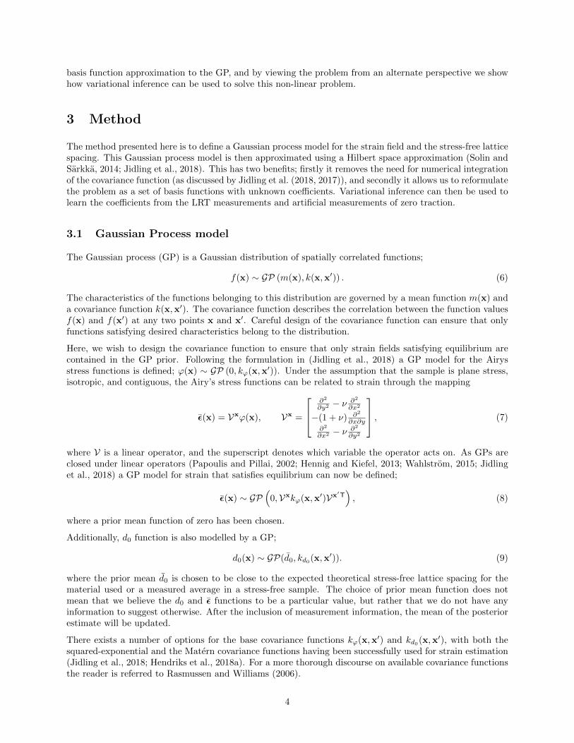
Here, we wish to design the covariance function to ensure that only strain fields satisfying equilibrium arecontained in the GP prior. Following the formulation in (Jidling et al., 2018) a GP model for the Airysstress functions is defined; ϕ(x) ∼ GP (0, kϕ(x,x′)). Under the assumption that the sample is plane stress,isotropic, and contiguous, the Airy’s stress functions can be related to strain through the mapping

ε(x) = Vxϕ(x), Vx =

∂2

∂y2 − ν∂2

∂x2

−(1 + ν) ∂2

∂x∂y∂2

∂x2 − ν ∂2

∂y2

, (7)

where V is a linear operator, and the superscript denotes which variable the operator acts on. As GPs areclosed under linear operators (Papoulis and Pillai, 2002; Hennig and Kiefel, 2013; Wahlstrom, 2015; Jidlinget al., 2018) a GP model for strain that satisfies equilibrium can now be defined;

ε(x) ∼ GP(

0,Vxkϕ(x,x′)Vx′T), (8)

where a prior mean function of zero has been chosen.

Additionally, d0 function is also modelled by a GP;

d0(x) ∼ GP(d0, kd0(x,x′)). (9)

where the prior mean d0 is chosen to be close to the expected theoretical stress-free lattice spacing for thematerial used or a measured average in a stress-free sample. The choice of prior mean function does notmean that we believe the d0 and ε functions to be a particular value, but rather that we do not have anyinformation to suggest otherwise. After the inclusion of measurement information, the mean of the posteriorestimate will be updated.

There exists a number of options for the base covariance functions kϕ(x,x′) and kd0(x,x′), with both thesquared-exponential and the Matern covariance functions having been successfully used for strain estimation(Jidling et al., 2018; Hendriks et al., 2018a). For a more thorough discourse on available covariance functionsthe reader is referred to Rasmussen and Williams (2006).

4

Having defined suitable GP models for the strain and d0 fields we now wish to estimate these fields from theLRT and traction measurements. However, the LRT is a non-linear function of these fields and consequentlya closed form solution does not exist. The following presents a method for obtaining these estimates thatapproximates the GP by a finite number of basis functions allowing variational inference to be applied.

3.2 Hilbert Space Approximation to the GP Prior

Here, we make use of the approximation method proposed by (Solin and Sarkka, 2014) and demonstratedto be suitable for the problem of strain tomography (Jidling et al., 2018). This method approximates ourcovariance function by a finite sum of m basis functions;

k(x,x′) =

m∑j=1

φi(x)S(λj)φj(x′), (10)

where S is the spectral density of the covariance function. For a stationary covariance function k = k(r),where r = x− x′, the spectral density and the basis functions are given by;

S(ω) =

∫k(r)e−iω

Tr dr, φj =1√LxLy

sin(λx,j(x+ Lx)) sin(λy,j(y + Ly)), (11)

where Lx and Ly control the domain size, and λ = [λx, λy]T encodes spatial frequencies of the basis functions.The basis functions are chosen as a solution to the Dirichlet boundary conditions on a rectangular domain,which is a natural choice for the Laplace eigenvalue problem that needs to be solved to approximate theGP (Jidling et al., 2018). The parameters θ = {lx, ly, σf} are commonly called ‘hyperparameters’ and canbe chosen by optimisation (as discussed in Section 5.2). For our application the domain size and spatialfrequencies are chosen such that the basis functions spanned a region where their spectral densities, weregreater than a minimum threshold. This helps to ensure that the dominant frequencies of the response arecaptured while maintaining numerical stability.

At this stage, the alternative view point of Bayesian linear regression can be taken. This approach modelsthe unknown function by a set of basis functions with Gaussian coefficients;

f(x) =

m∑j=1

φj(x)wj = φ(x)w, wj ∼ N (µj , S(λj)), (12)

where φ(x) and w have dimensions [1,m] and [m, 1], respectively. This gives the following model for thestrain field ε(x) and the stress-free lattice spacing d0(x);

ε∗(x) = φεwϕ, φε,j(x) = Vxφϕ,j(x), φϕ,j =1√

LϕxLϕysin(λϕx,j(x+ Lϕx)) sin(λϕy,j(y + Lϕy)),

d0∗(x) = φd0wd0 , φd0,k(x) =1√

Ld0xLd0ysin(λd0x,k(x+ Ld0x)) sin(λd0y,k(y + Ld0y)),

(13)

where the unknown coefficients are independently normally distributed to approximate our GP model; wϕ,j ∼N (0, Sϕ(λϕ,j)) and wd0,j ∼ N (µd0,j , Sd0(λd0,j)). Where the means µd0,j are chosen so that the prior has theconstant value d0. In this work, basis functions and parameters corresponding to the d0 field will be denotedby the subscript d0 and the subscript k will be used as an index. Likewise, basis functions and parameterscorresponding to the Airys stress function will be denoted by the subscript d0 and the subscript j will beused as an index. The expanded expressions for φε are given in Appendix A.

Using the LRT (3) we can write a model for a predicted measurement as a non-linear function of the unknowncoefficients;

y∗ =1

L

L∫0

n

∑j

∑k

φε,j(p + ns)wϕ,jφd0,k(p + ns)wd0,k

+

(∑k

φd0,k(p + ns)wd0,k

)ds

= gy(wϕ,wd0 ,η),

(14)

5

where we have restricted ourselves to a single measurement to simplify the notation. These integrals canbe analytically evaluated and the equations are given in Appendix A. Predictions of the boundary tractionsyt at a boundary location xb with surface normal n⊥ can be written as a linear function of the unknowncoefficients;

yt∗ =

[n⊥1 n⊥2 0

0 n⊥1 n⊥2

]︸ ︷︷ ︸

T

φϕ(x)wϕ = T(n⊥)φϕ(xb)wϕ

= gt(w,xb,n⊥).

(15)

The coefficients wϕ and wd0 are random variables; as such the predictions ε∗, y∗, and yt∗ are also randomvariables. The problem now is to determine the distribution of the coefficients given a set of LRT and tractionmeasurements. This problem is now in a form allowing variational inference to be used to approximate asolution to the non-linear problem.

3.3 Variational Inference

Variational inference (Blei et al., 2017; Jordan et al., 1999) provides an approximation to the posteriordistribution by assuming that it has a certain functional form that contain unknown parameters. Theseunknown parameters are found using optimization, where some distance measure is minimized. We will inthis section provide the details enabling the use of variational inference in solving our problem.

Given n transmission measurements and nt traction measurements, such that a vector of all measurementsis given by Y = [y1, . . . , yn, yt,1, . . . , yt,nt ]

T, the problem can be written as having prior and likelihood

p(w) ∼ N (µ,Σp) and p(Y|w) ∼ N (Y|g(w),Σn), (16)

where w =[wTd0

wTϕ

]T, µ is a vector of all the prior means, and Σp is a matrix with the coefficients prior

variance on the diagonals. Here, g(·) is the combined measurement model that expresses the measurementvector Y as a function of the coefficients. This function is constructed using both (14) and (15). Finally,Σn = diag(σ2

nIn×n, σ2t Int×nt), where σ2

t is a small variance placed on the artificial traction measurementsadded for numerical reasons.

The non-linear measurement function g(·) makes the likelihood intractable as the prior and likelihood areno longer conjugate. Consequently, the posterior p(w|Y) is also intractable and so we find an approximatesolution using variational inference (Jordan et al., 1999). The idea is to approximate the true posterior bythe Gaussian distribution q(w) ∼ N (w,C), and find the mean w and covariance C for this distribution thatmaximise the Free Energy F . The Free Energy places a lower bound on the log marginal likelihood andhence provides a measure of how well our posterior fits the data;

log p(Y) ≥ E [log p(Y|W)]−KL [q(w)||p(w|Y)] = F (17)

where, in this case, E[·] is the expected value with respect to the approximate posterior q(w) and KL[·] isthe Kullback Leibler divergence which provides a measure of difference between the approximate posteriorand the true posterior. These terms can be evaluated as (Steinberg and Bonilla, 2014);

E [log p(Y|W)] =1

2

[N log 2π + log |Σn|+ (Y − E [g(w)])TΣ−1n (Y − E [g(w)])

],

KL [q(w)||p(w|Y)] =1

2

[tr(Σ−1p C) + (µ− w)

TΣ−1p (µ− w)− log |C|+ log |Σp| −N

],

(18)

where N = n + nt. Here, the expectation of the non-linear function E [g(w)] is intractable (Steinberg and

Bonilla, 2014) and so the expected maximum is used Y = g(w);

F ≈ −1

2

[N log 2π + log |Σn| − log |C|+ log |Σp|+ (Y − g(w))TΣ−1

n (Y − g(w)) + (µ− w)T Σ−1p (µ− w)

](19)

6

The optimal posterior mean is chosen to maximise the Free Energy. To perform this optimisation a modifiedNewton’s method is used where the step direction is q = −H−1g and we can calculate the gradient, g, andHessian, H, of the cost as

g = JTΣ−1n (Y − g(w))−Σ−1p w

H = −JTΣ−1n J +∂JT

∂wΣ−1n (Y − g(w))−Σ−1p

(20)

where J =[∂Y∂w

T∂Yt

∂w

T]T

, and the derivatives and second derivatives are given in Appendix B. At each

iteration we update the coefficients according to

wk+1 = (1− α)wk + αq + αµ, (21)

A backwards line search is used to ensure that F is increased in each iteration. Once the optimal posteriormean is found, the covariance can be found by setting ∂F

∂C = 0 and linearising about w (Steinberg and Bonilla,2014), giving;

C =[Σ−1p + JTΣ−1n J

]−1. (22)

Pseudo-code for an algorithm to find approximate distribution of the coefficients q(w) ∼ N (w,C) is givenin Algorithm 1. Once the coefficients are found, estimates of the strain and d0 fields can be estimated. Theapproximate poster mean and variance for the strain field and stress-free lattice spacing can be computed as[

d0(x)ˆε

]=

[φε(x) 0

0 φε(x)

]w,

Σ =

[φε(x) 0

0 φε(x)

]C

[φε(x) 0

0 φε(x)

]T,

(23)

where Σ is the joint covariance of the strain and d0 estimates. Next, this method is demonstrated on a setof measurements simulated from a theoretical cantilever beam strain field and an artificial d0 field.

Algorithm 1 Variational inference algorithm for finding the coefficients q(w) ∼ N (w,C). Requires thehyperparameters θ, the specified number of basis functions mϕ and md0 , the LRT measurement information{yi,ηi|∀i = 1, . . . , n} and the boundary traction information {yt,i = 0,xb,i,n⊥,i|∀i = 1, . . . , nt}.

1: procedure Find Coefficients2: Compute the basis functions for the LRT measurements using Equation 143: Compute the basis functions for the traction measurements using Equation 154: Build prior variance Σp

5: Initialise the coefficients w1

6: set k = 17: while Stopping criteria not met do8: Compute the gradient g and Hessian H linearised about wk according to Equation 209: Calculate wk+1 using Equation 21 and a backward line search

10: k = k + 111: end while12: Calculate the covariance C according to Equation 2213: return wk and C14: end procedure

4 Simulation Results

The method’s ability to jointly reconstruct the strain field and a d0 field is demonstrated using simulatedmeasurements. Reconstructions from measurements simulated through two strain fields is shown; the Saint-Venant approximate strain field for a cantilver beam, and a Finite Element Analysis (FEA) strain field from

7

an in-situ loaded C-shape. Additionally, the consequences of ignoring the d0 variation on the reconstructionare shown by using the linear measurement model and Gaussian process regression method presented byJidling et al. (2018) with the addition of traction constraints as shown in Hendriks et al. (2018a). Matlabcode to run both examples can be found on Github (Hendriks, 2019).

4.1 Cantilever Beam Example

The method is first demonstrated for the theoretical Saint-Venant cantilever beam as studied. Assumingplane stress, the Saint-Venant approximation to the strain field is (Beer et al., 2010):

E(x) =

PEI (L− x)y

− (1+ν)P2EI

((h2

)2 − y2)−νPEI (L− x)y

, (24)

where the geometry is defined in Figure 2. A synthetic stress-free lattice spacing field is defined by

d0(x) = c0 exp

(−1

2(x− c1)2/c22 −

1

2(y − c3)2/c24

)+ c5, (25)

with the parameters given by {c0, c1, c2, c3, c4, c5} = {0.0168, 0, 7.5 × 10−3, 7 × 10−3, 6 × 10−3, 4.056}. Themaximum variation c0 from a constant base value, c5, was chosen to reflect the possible maximum relativevariation due to martensitic phase change in 0.8% carbon steel.

h<latexit sha1_base64="tznJ5l2ae4xkmpo8iX0nAmXub7k=">AAAB6HicbVBNS8NAEJ3Ur1q/qh69LBbBU0lEaI8FLx5bsB/QhrLZTtq1m03Y3Qgl9Bd48aCIV3+SN/+N2zYHbX0w8Hhvhpl5QSK4Nq777RS2tnd294r7pYPDo+OT8ulZR8epYthmsYhVL6AaBZfYNtwI7CUKaRQI7AbTu4XffUKleSwfzCxBP6JjyUPOqLFSazIsV9yquwTZJF5OKpCjOSx/DUYxSyOUhgmqdd9zE+NnVBnOBM5Lg1RjQtmUjrFvqaQRaj9bHjonV1YZkTBWtqQhS/X3REYjrWdRYDsjaiZ63VuI/3n91IR1P+MySQ1KtloUpoKYmCy+JiOukBkxs4Qyxe2thE2ooszYbEo2BG/95U3Sual6btVr3VYa9TyOIlzAJVyDBzVowD00oQ0MEJ7hFd6cR+fFeXc+Vq0FJ585hz9wPn8AyveM4g==</latexit><latexit sha1_base64="tznJ5l2ae4xkmpo8iX0nAmXub7k=">AAAB6HicbVBNS8NAEJ3Ur1q/qh69LBbBU0lEaI8FLx5bsB/QhrLZTtq1m03Y3Qgl9Bd48aCIV3+SN/+N2zYHbX0w8Hhvhpl5QSK4Nq777RS2tnd294r7pYPDo+OT8ulZR8epYthmsYhVL6AaBZfYNtwI7CUKaRQI7AbTu4XffUKleSwfzCxBP6JjyUPOqLFSazIsV9yquwTZJF5OKpCjOSx/DUYxSyOUhgmqdd9zE+NnVBnOBM5Lg1RjQtmUjrFvqaQRaj9bHjonV1YZkTBWtqQhS/X3REYjrWdRYDsjaiZ63VuI/3n91IR1P+MySQ1KtloUpoKYmCy+JiOukBkxs4Qyxe2thE2ooszYbEo2BG/95U3Sual6btVr3VYa9TyOIlzAJVyDBzVowD00oQ0MEJ7hFd6cR+fFeXc+Vq0FJ585hz9wPn8AyveM4g==</latexit><latexit sha1_base64="tznJ5l2ae4xkmpo8iX0nAmXub7k=">AAAB6HicbVBNS8NAEJ3Ur1q/qh69LBbBU0lEaI8FLx5bsB/QhrLZTtq1m03Y3Qgl9Bd48aCIV3+SN/+N2zYHbX0w8Hhvhpl5QSK4Nq777RS2tnd294r7pYPDo+OT8ulZR8epYthmsYhVL6AaBZfYNtwI7CUKaRQI7AbTu4XffUKleSwfzCxBP6JjyUPOqLFSazIsV9yquwTZJF5OKpCjOSx/DUYxSyOUhgmqdd9zE+NnVBnOBM5Lg1RjQtmUjrFvqaQRaj9bHjonV1YZkTBWtqQhS/X3REYjrWdRYDsjaiZ63VuI/3n91IR1P+MySQ1KtloUpoKYmCy+JiOukBkxs4Qyxe2thE2ooszYbEo2BG/95U3Sual6btVr3VYa9TyOIlzAJVyDBzVowD00oQ0MEJ7hFd6cR+fFeXc+Vq0FJ585hz9wPn8AyveM4g==</latexit><latexit sha1_base64="tznJ5l2ae4xkmpo8iX0nAmXub7k=">AAAB6HicbVBNS8NAEJ3Ur1q/qh69LBbBU0lEaI8FLx5bsB/QhrLZTtq1m03Y3Qgl9Bd48aCIV3+SN/+N2zYHbX0w8Hhvhpl5QSK4Nq777RS2tnd294r7pYPDo+OT8ulZR8epYthmsYhVL6AaBZfYNtwI7CUKaRQI7AbTu4XffUKleSwfzCxBP6JjyUPOqLFSazIsV9yquwTZJF5OKpCjOSx/DUYxSyOUhgmqdd9zE+NnVBnOBM5Lg1RjQtmUjrFvqaQRaj9bHjonV1YZkTBWtqQhS/X3REYjrWdRYDsjaiZ63VuI/3n91IR1P+MySQ1KtloUpoKYmCy+JiOukBkxs4Qyxe2thE2ooszYbEo2BG/95U3Sual6btVr3VYa9TyOIlzAJVyDBzVowD00oQ0MEJ7hFd6cR+fFeXc+Vq0FJ585hz9wPn8AyveM4g==</latexit>

l<latexit sha1_base64="wy0EiCbXlRZnjxe0JHZa2rKsBmI=">AAAB6HicbVBNS8NAEJ3Ur1q/qh69LBbBU0lEaI8FLx5bsB/QhrLZTtq1m03Y3Qgl9Bd48aCIV3+SN/+N2zYHbX0w8Hhvhpl5QSK4Nq777RS2tnd294r7pYPDo+OT8ulZR8epYthmsYhVL6AaBZfYNtwI7CUKaRQI7AbTu4XffUKleSwfzCxBP6JjyUPOqLFSSwzLFbfqLkE2iZeTCuRoDstfg1HM0gilYYJq3ffcxPgZVYYzgfPSINWYUDalY+xbKmmE2s+Wh87JlVVGJIyVLWnIUv09kdFI61kU2M6Imole9xbif14/NWHdz7hMUoOSrRaFqSAmJouvyYgrZEbMLKFMcXsrYROqKDM2m5INwVt/eZN0bqqeW/Vat5VGPY+jCBdwCdfgQQ0acA9NaAMDhGd4hTfn0Xlx3p2PVWvByWfO4Q+czx/RB4zm</latexit><latexit sha1_base64="wy0EiCbXlRZnjxe0JHZa2rKsBmI=">AAAB6HicbVBNS8NAEJ3Ur1q/qh69LBbBU0lEaI8FLx5bsB/QhrLZTtq1m03Y3Qgl9Bd48aCIV3+SN/+N2zYHbX0w8Hhvhpl5QSK4Nq777RS2tnd294r7pYPDo+OT8ulZR8epYthmsYhVL6AaBZfYNtwI7CUKaRQI7AbTu4XffUKleSwfzCxBP6JjyUPOqLFSSwzLFbfqLkE2iZeTCuRoDstfg1HM0gilYYJq3ffcxPgZVYYzgfPSINWYUDalY+xbKmmE2s+Wh87JlVVGJIyVLWnIUv09kdFI61kU2M6Imole9xbif14/NWHdz7hMUoOSrRaFqSAmJouvyYgrZEbMLKFMcXsrYROqKDM2m5INwVt/eZN0bqqeW/Vat5VGPY+jCBdwCdfgQQ0acA9NaAMDhGd4hTfn0Xlx3p2PVWvByWfO4Q+czx/RB4zm</latexit><latexit sha1_base64="wy0EiCbXlRZnjxe0JHZa2rKsBmI=">AAAB6HicbVBNS8NAEJ3Ur1q/qh69LBbBU0lEaI8FLx5bsB/QhrLZTtq1m03Y3Qgl9Bd48aCIV3+SN/+N2zYHbX0w8Hhvhpl5QSK4Nq777RS2tnd294r7pYPDo+OT8ulZR8epYthmsYhVL6AaBZfYNtwI7CUKaRQI7AbTu4XffUKleSwfzCxBP6JjyUPOqLFSSwzLFbfqLkE2iZeTCuRoDstfg1HM0gilYYJq3ffcxPgZVYYzgfPSINWYUDalY+xbKmmE2s+Wh87JlVVGJIyVLWnIUv09kdFI61kU2M6Imole9xbif14/NWHdz7hMUoOSrRaFqSAmJouvyYgrZEbMLKFMcXsrYROqKDM2m5INwVt/eZN0bqqeW/Vat5VGPY+jCBdwCdfgQQ0acA9NaAMDhGd4hTfn0Xlx3p2PVWvByWfO4Q+czx/RB4zm</latexit><latexit sha1_base64="wy0EiCbXlRZnjxe0JHZa2rKsBmI=">AAAB6HicbVBNS8NAEJ3Ur1q/qh69LBbBU0lEaI8FLx5bsB/QhrLZTtq1m03Y3Qgl9Bd48aCIV3+SN/+N2zYHbX0w8Hhvhpl5QSK4Nq777RS2tnd294r7pYPDo+OT8ulZR8epYthmsYhVL6AaBZfYNtwI7CUKaRQI7AbTu4XffUKleSwfzCxBP6JjyUPOqLFSSwzLFbfqLkE2iZeTCuRoDstfg1HM0gilYYJq3ffcxPgZVYYzgfPSINWYUDalY+xbKmmE2s+Wh87JlVVGJIyVLWnIUv09kdFI61kU2M6Imole9xbif14/NWHdz7hMUoOSrRaFqSAmJouvyYgrZEbMLKFMcXsrYROqKDM2m5INwVt/eZN0bqqeW/Vat5VGPY+jCBdwCdfgQQ0acA9NaAMDhGd4hTfn0Xlx3p2PVWvByWfO4Q+czx/RB4zm</latexit>

P<latexit sha1_base64="hKSgFSD7v8QS+Xn0xIkMciP3fvA=">AAAB6HicbVDLSsNAFL2pr1pfVZduBovgqiQi2GXBjcsW7APaIJPpTTt2MgkzE6GEfoEbF4q49ZPc+TdO2iy09cDA4ZxzmXtPkAiujet+O6WNza3tnfJuZW//4PCoenzS1XGqGHZYLGLVD6hGwSV2DDcC+4lCGgUCe8H0Nvd7T6g0j+W9mSXoR3QsecgZNVZqtx6qNbfuLkDWiVeQGhSw+a/hKGZphNIwQbUeeG5i/Iwqw5nAeWWYakwom9IxDiyVNELtZ4tF5+TCKiMSxso+achC/T2R0UjrWRTYZETNRK96ufifN0hN2PAzLpPUoGTLj8JUEBOT/Goy4gqZETNLKFPc7krYhCrKjO2mYkvwVk9eJ92ruufWvfZ1rdko6ijDGZzDJXhwA024gxZ0gAHCM7zCm/PovDjvzscyWnKKmVP4A+fzB6aXjMo=</latexit><latexit sha1_base64="hKSgFSD7v8QS+Xn0xIkMciP3fvA=">AAAB6HicbVDLSsNAFL2pr1pfVZduBovgqiQi2GXBjcsW7APaIJPpTTt2MgkzE6GEfoEbF4q49ZPc+TdO2iy09cDA4ZxzmXtPkAiujet+O6WNza3tnfJuZW//4PCoenzS1XGqGHZYLGLVD6hGwSV2DDcC+4lCGgUCe8H0Nvd7T6g0j+W9mSXoR3QsecgZNVZqtx6qNbfuLkDWiVeQGhSw+a/hKGZphNIwQbUeeG5i/Iwqw5nAeWWYakwom9IxDiyVNELtZ4tF5+TCKiMSxso+achC/T2R0UjrWRTYZETNRK96ufifN0hN2PAzLpPUoGTLj8JUEBOT/Goy4gqZETNLKFPc7krYhCrKjO2mYkvwVk9eJ92ruufWvfZ1rdko6ijDGZzDJXhwA024gxZ0gAHCM7zCm/PovDjvzscyWnKKmVP4A+fzB6aXjMo=</latexit><latexit sha1_base64="hKSgFSD7v8QS+Xn0xIkMciP3fvA=">AAAB6HicbVDLSsNAFL2pr1pfVZduBovgqiQi2GXBjcsW7APaIJPpTTt2MgkzE6GEfoEbF4q49ZPc+TdO2iy09cDA4ZxzmXtPkAiujet+O6WNza3tnfJuZW//4PCoenzS1XGqGHZYLGLVD6hGwSV2DDcC+4lCGgUCe8H0Nvd7T6g0j+W9mSXoR3QsecgZNVZqtx6qNbfuLkDWiVeQGhSw+a/hKGZphNIwQbUeeG5i/Iwqw5nAeWWYakwom9IxDiyVNELtZ4tF5+TCKiMSxso+achC/T2R0UjrWRTYZETNRK96ufifN0hN2PAzLpPUoGTLj8JUEBOT/Goy4gqZETNLKFPc7krYhCrKjO2mYkvwVk9eJ92ruufWvfZ1rdko6ijDGZzDJXhwA024gxZ0gAHCM7zCm/PovDjvzscyWnKKmVP4A+fzB6aXjMo=</latexit><latexit sha1_base64="hP+6LrUf2d3tZaldqaQQvEKMXyw=">AAAB2XicbZDNSgMxFIXv1L86Vq1rN8EiuCozbnQpuHFZwbZCO5RM5k4bmskMyR2hDH0BF25EfC93vo3pz0JbDwQ+zknIvSculLQUBN9ebWd3b/+gfugfNfzjk9Nmo2fz0gjsilzl5jnmFpXU2CVJCp8LgzyLFfbj6f0i77+gsTLXTzQrMMr4WMtUCk7O6oyaraAdLMW2IVxDC9YaNb+GSS7KDDUJxa0dhEFBUcUNSaFw7g9LiwUXUz7GgUPNM7RRtRxzzi6dk7A0N+5oYkv394uKZ9bOstjdzDhN7Ga2MP/LBiWlt1EldVESarH6KC0Vo5wtdmaJNChIzRxwYaSblYkJN1yQa8Z3HYSbG29D77odBu3wMYA6nMMFXEEIN3AHD9CBLghI4BXevYn35n2suqp569LO4I+8zx84xIo4</latexit><latexit sha1_base64="tnntUTxXcxOWd0f4qj9iCThv/j4=">AAAB3XicbVDLSgNBEOyNrxijRq9eBoPgKex60aPgxWMC5gHJIrOT3mTM7Owy0yuEJV/gxYMi/pY3/8bJ46CJBQ1FVTfdXVGmpCXf//ZKW9s7u3vl/cpB9fDouHZS7dg0NwLbIlWp6UXcopIa2yRJYS8zyJNIYTea3M397jMaK1P9QNMMw4SPtIyl4OSkVvOxVvcb/gJskwQrUocVXP/XYJiKPEFNQnFr+4GfUVhwQ1IonFUGucWMiwkfYd9RzRO0YbE4dMYunDJkcWpcaWIL9fdEwRNrp0nkOhNOY7vuzcX/vH5O8U1YSJ3lhFosF8W5YpSy+ddsKA0KUlNHuDDS3crEmBsuyGVTcSEE6y9vks5VI/AbQcuHMpzBOVxCANdwC/fQhDYIQHiBN3j3nrxX72MZV8lb5XYKf+B9/gCWq4uB</latexit><latexit sha1_base64="tnntUTxXcxOWd0f4qj9iCThv/j4=">AAAB3XicbVDLSgNBEOyNrxijRq9eBoPgKex60aPgxWMC5gHJIrOT3mTM7Owy0yuEJV/gxYMi/pY3/8bJ46CJBQ1FVTfdXVGmpCXf//ZKW9s7u3vl/cpB9fDouHZS7dg0NwLbIlWp6UXcopIa2yRJYS8zyJNIYTea3M397jMaK1P9QNMMw4SPtIyl4OSkVvOxVvcb/gJskwQrUocVXP/XYJiKPEFNQnFr+4GfUVhwQ1IonFUGucWMiwkfYd9RzRO0YbE4dMYunDJkcWpcaWIL9fdEwRNrp0nkOhNOY7vuzcX/vH5O8U1YSJ3lhFosF8W5YpSy+ddsKA0KUlNHuDDS3crEmBsuyGVTcSEE6y9vks5VI/AbQcuHMpzBOVxCANdwC/fQhDYIQHiBN3j3nrxX72MZV8lb5XYKf+B9/gCWq4uB</latexit><latexit sha1_base64="XnW/X7TDMpuoFcQG2IPMeXVcIkQ=">AAAB6HicbVDLSgMxFL3js9ZX1aWbYBFclYwbuyy4cdmCfUA7SCa908ZmMkOSEcrQL3DjQhG3fpI7/8a0nYW2HggczjmX3HvCVApjKf32Nja3tnd2S3vl/YPDo+PKyWnHJJnm2OaJTHQvZAalUNi2wkrspRpZHErshpPbud99Qm1Eou7tNMUgZiMlIsGZdVKr+VCp0hpdgKwTvyBVKODyX4NhwrMYleWSGdP3aWqDnGkruMRZeZAZTBmfsBH2HVUsRhPki0Vn5NIpQxIl2j1lyUL9PZGz2JhpHLpkzOzYrHpz8T+vn9moHuRCpZlFxZcfRZkkNiHzq8lQaORWTh1hXAu3K+Fjphm3rpuyK8FfPXmddK5rPq35LVpt1Is6SnAOF3AFPtxAA+6gCW3ggPAMr/DmPXov3rv3sYxueMXMGfyB9/kDpVeMxg==</latexit><latexit sha1_base64="hKSgFSD7v8QS+Xn0xIkMciP3fvA=">AAAB6HicbVDLSsNAFL2pr1pfVZduBovgqiQi2GXBjcsW7APaIJPpTTt2MgkzE6GEfoEbF4q49ZPc+TdO2iy09cDA4ZxzmXtPkAiujet+O6WNza3tnfJuZW//4PCoenzS1XGqGHZYLGLVD6hGwSV2DDcC+4lCGgUCe8H0Nvd7T6g0j+W9mSXoR3QsecgZNVZqtx6qNbfuLkDWiVeQGhSw+a/hKGZphNIwQbUeeG5i/Iwqw5nAeWWYakwom9IxDiyVNELtZ4tF5+TCKiMSxso+achC/T2R0UjrWRTYZETNRK96ufifN0hN2PAzLpPUoGTLj8JUEBOT/Goy4gqZETNLKFPc7krYhCrKjO2mYkvwVk9eJ92ruufWvfZ1rdko6ijDGZzDJXhwA024gxZ0gAHCM7zCm/PovDjvzscyWnKKmVP4A+fzB6aXjMo=</latexit><latexit sha1_base64="hKSgFSD7v8QS+Xn0xIkMciP3fvA=">AAAB6HicbVDLSsNAFL2pr1pfVZduBovgqiQi2GXBjcsW7APaIJPpTTt2MgkzE6GEfoEbF4q49ZPc+TdO2iy09cDA4ZxzmXtPkAiujet+O6WNza3tnfJuZW//4PCoenzS1XGqGHZYLGLVD6hGwSV2DDcC+4lCGgUCe8H0Nvd7T6g0j+W9mSXoR3QsecgZNVZqtx6qNbfuLkDWiVeQGhSw+a/hKGZphNIwQbUeeG5i/Iwqw5nAeWWYakwom9IxDiyVNELtZ4tF5+TCKiMSxso+achC/T2R0UjrWRTYZETNRK96ufifN0hN2PAzLpPUoGTLj8JUEBOT/Goy4gqZETNLKFPc7krYhCrKjO2mYkvwVk9eJ92ruufWvfZ1rdko6ijDGZzDJXhwA024gxZ0gAHCM7zCm/PovDjvzscyWnKKmVP4A+fzB6aXjMo=</latexit><latexit sha1_base64="hKSgFSD7v8QS+Xn0xIkMciP3fvA=">AAAB6HicbVDLSsNAFL2pr1pfVZduBovgqiQi2GXBjcsW7APaIJPpTTt2MgkzE6GEfoEbF4q49ZPc+TdO2iy09cDA4ZxzmXtPkAiujet+O6WNza3tnfJuZW//4PCoenzS1XGqGHZYLGLVD6hGwSV2DDcC+4lCGgUCe8H0Nvd7T6g0j+W9mSXoR3QsecgZNVZqtx6qNbfuLkDWiVeQGhSw+a/hKGZphNIwQbUeeG5i/Iwqw5nAeWWYakwom9IxDiyVNELtZ4tF5+TCKiMSxso+achC/T2R0UjrWRTYZETNRK96ufifN0hN2PAzLpPUoGTLj8JUEBOT/Goy4gqZETNLKFPc7krYhCrKjO2mYkvwVk9eJ92ruufWvfZ1rdko6ijDGZzDJXhwA024gxZ0gAHCM7zCm/PovDjvzscyWnKKmVP4A+fzB6aXjMo=</latexit><latexit sha1_base64="hKSgFSD7v8QS+Xn0xIkMciP3fvA=">AAAB6HicbVDLSsNAFL2pr1pfVZduBovgqiQi2GXBjcsW7APaIJPpTTt2MgkzE6GEfoEbF4q49ZPc+TdO2iy09cDA4ZxzmXtPkAiujet+O6WNza3tnfJuZW//4PCoenzS1XGqGHZYLGLVD6hGwSV2DDcC+4lCGgUCe8H0Nvd7T6g0j+W9mSXoR3QsecgZNVZqtx6qNbfuLkDWiVeQGhSw+a/hKGZphNIwQbUeeG5i/Iwqw5nAeWWYakwom9IxDiyVNELtZ4tF5+TCKiMSxso+achC/T2R0UjrWRTYZETNRK96ufifN0hN2PAzLpPUoGTLj8JUEBOT/Goy4gqZETNLKFPc7krYhCrKjO2mYkvwVk9eJ92ruufWvfZ1rdko6ijDGZzDJXhwA024gxZ0gAHCM7zCm/PovDjvzscyWnKKmVP4A+fzB6aXjMo=</latexit><latexit sha1_base64="hKSgFSD7v8QS+Xn0xIkMciP3fvA=">AAAB6HicbVDLSsNAFL2pr1pfVZduBovgqiQi2GXBjcsW7APaIJPpTTt2MgkzE6GEfoEbF4q49ZPc+TdO2iy09cDA4ZxzmXtPkAiujet+O6WNza3tnfJuZW//4PCoenzS1XGqGHZYLGLVD6hGwSV2DDcC+4lCGgUCe8H0Nvd7T6g0j+W9mSXoR3QsecgZNVZqtx6qNbfuLkDWiVeQGhSw+a/hKGZphNIwQbUeeG5i/Iwqw5nAeWWYakwom9IxDiyVNELtZ4tF5+TCKiMSxso+achC/T2R0UjrWRTYZETNRK96ufifN0hN2PAzLpPUoGTLj8JUEBOT/Goy4gqZETNLKFPc7krYhCrKjO2mYkvwVk9eJ92ruufWvfZ1rdko6ijDGZzDJXhwA024gxZ0gAHCM7zCm/PovDjvzscyWnKKmVP4A+fzB6aXjMo=</latexit><latexit sha1_base64="hKSgFSD7v8QS+Xn0xIkMciP3fvA=">AAAB6HicbVDLSsNAFL2pr1pfVZduBovgqiQi2GXBjcsW7APaIJPpTTt2MgkzE6GEfoEbF4q49ZPc+TdO2iy09cDA4ZxzmXtPkAiujet+O6WNza3tnfJuZW//4PCoenzS1XGqGHZYLGLVD6hGwSV2DDcC+4lCGgUCe8H0Nvd7T6g0j+W9mSXoR3QsecgZNVZqtx6qNbfuLkDWiVeQGhSw+a/hKGZphNIwQbUeeG5i/Iwqw5nAeWWYakwom9IxDiyVNELtZ4tF5+TCKiMSxso+achC/T2R0UjrWRTYZETNRK96ufifN0hN2PAzLpPUoGTLj8JUEBOT/Goy4gqZETNLKFPc7krYhCrKjO2mYkvwVk9eJ92ruufWvfZ1rdko6ijDGZzDJXhwA024gxZ0gAHCM7zCm/PovDjvzscyWnKKmVP4A+fzB6aXjMo=</latexit>

x<latexit sha1_base64="sS/1Y4RUFRdYgUjEZXi7AEhWI1A=">AAAB6HicbVBNS8NAEJ3Ur1q/qh69LBbBU0lEsMeCF48t2A9oQ9lsJ+3azSbsbsQS+gu8eFDEqz/Jm//GbZuDtj4YeLw3w8y8IBFcG9f9dgobm1vbO8Xd0t7+weFR+fikreNUMWyxWMSqG1CNgktsGW4EdhOFNAoEdoLJ7dzvPKLSPJb3ZpqgH9GR5CFn1Fip+TQoV9yquwBZJ15OKpCjMSh/9YcxSyOUhgmqdc9zE+NnVBnOBM5K/VRjQtmEjrBnqaQRaj9bHDojF1YZkjBWtqQhC/X3REYjradRYDsjasZ61ZuL/3m91IQ1P+MySQ1KtlwUpoKYmMy/JkOukBkxtYQyxe2thI2poszYbEo2BG/15XXSvqp6btVrXlfqtTyOIpzBOVyCBzdQhztoQAsYIDzDK7w5D86L8+58LFsLTj5zCn/gfP4A4zeM8g==</latexit><latexit sha1_base64="sS/1Y4RUFRdYgUjEZXi7AEhWI1A=">AAAB6HicbVBNS8NAEJ3Ur1q/qh69LBbBU0lEsMeCF48t2A9oQ9lsJ+3azSbsbsQS+gu8eFDEqz/Jm//GbZuDtj4YeLw3w8y8IBFcG9f9dgobm1vbO8Xd0t7+weFR+fikreNUMWyxWMSqG1CNgktsGW4EdhOFNAoEdoLJ7dzvPKLSPJb3ZpqgH9GR5CFn1Fip+TQoV9yquwBZJ15OKpCjMSh/9YcxSyOUhgmqdc9zE+NnVBnOBM5K/VRjQtmEjrBnqaQRaj9bHDojF1YZkjBWtqQhC/X3REYjradRYDsjasZ61ZuL/3m91IQ1P+MySQ1KtlwUpoKYmMy/JkOukBkxtYQyxe2thI2poszYbEo2BG/15XXSvqp6btVrXlfqtTyOIpzBOVyCBzdQhztoQAsYIDzDK7w5D86L8+58LFsLTj5zCn/gfP4A4zeM8g==</latexit><latexit sha1_base64="sS/1Y4RUFRdYgUjEZXi7AEhWI1A=">AAAB6HicbVBNS8NAEJ3Ur1q/qh69LBbBU0lEsMeCF48t2A9oQ9lsJ+3azSbsbsQS+gu8eFDEqz/Jm//GbZuDtj4YeLw3w8y8IBFcG9f9dgobm1vbO8Xd0t7+weFR+fikreNUMWyxWMSqG1CNgktsGW4EdhOFNAoEdoLJ7dzvPKLSPJb3ZpqgH9GR5CFn1Fip+TQoV9yquwBZJ15OKpCjMSh/9YcxSyOUhgmqdc9zE+NnVBnOBM5K/VRjQtmEjrBnqaQRaj9bHDojF1YZkjBWtqQhC/X3REYjradRYDsjasZ61ZuL/3m91IQ1P+MySQ1KtlwUpoKYmMy/JkOukBkxtYQyxe2thI2poszYbEo2BG/15XXSvqp6btVrXlfqtTyOIpzBOVyCBzdQhztoQAsYIDzDK7w5D86L8+58LFsLTj5zCn/gfP4A4zeM8g==</latexit><latexit sha1_base64="hP+6LrUf2d3tZaldqaQQvEKMXyw=">AAAB2XicbZDNSgMxFIXv1L86Vq1rN8EiuCozbnQpuHFZwbZCO5RM5k4bmskMyR2hDH0BF25EfC93vo3pz0JbDwQ+zknIvSculLQUBN9ebWd3b/+gfugfNfzjk9Nmo2fz0gjsilzl5jnmFpXU2CVJCp8LgzyLFfbj6f0i77+gsTLXTzQrMMr4WMtUCk7O6oyaraAdLMW2IVxDC9YaNb+GSS7KDDUJxa0dhEFBUcUNSaFw7g9LiwUXUz7GgUPNM7RRtRxzzi6dk7A0N+5oYkv394uKZ9bOstjdzDhN7Ga2MP/LBiWlt1EldVESarH6KC0Vo5wtdmaJNChIzRxwYaSblYkJN1yQa8Z3HYSbG29D77odBu3wMYA6nMMFXEEIN3AHD9CBLghI4BXevYn35n2suqp569LO4I+8zx84xIo4</latexit><latexit sha1_base64="u83j/XzZ2ZMt9PzkJ56wspYVcvA=">AAAB3XicbZBLSwMxFIXv1FetVatbN8EiuCozbnQpuHHZgn1AW0omvdPGZjJDckcsQ3+BGxeK+Lfc+W9MHwttPRD4OCch954wVdKS7397ha3tnd294n7poHx4dFw5KbdskhmBTZGoxHRCblFJjU2SpLCTGuRxqLAdTu7mefsJjZWJfqBpiv2Yj7SMpODkrMbzoFL1a/5CbBOCFVRhpfqg8tUbJiKLUZNQ3Npu4KfUz7khKRTOSr3MYsrFhI+w61DzGG0/Xww6YxfOGbIoMe5oYgv394ucx9ZO49DdjDmN7Xo2N//LuhlFN/1c6jQj1GL5UZQpRgmbb82G0qAgNXXAhZFuVibG3HBBrpuSKyFYX3kTWle1wK8FDR+KcAbncAkBXMMt3EMdmiAA4QXe4N179F69j2VdBW/V2yn8kff5A9GTi6k=</latexit><latexit sha1_base64="u83j/XzZ2ZMt9PzkJ56wspYVcvA=">AAAB3XicbZBLSwMxFIXv1FetVatbN8EiuCozbnQpuHHZgn1AW0omvdPGZjJDckcsQ3+BGxeK+Lfc+W9MHwttPRD4OCch954wVdKS7397ha3tnd294n7poHx4dFw5KbdskhmBTZGoxHRCblFJjU2SpLCTGuRxqLAdTu7mefsJjZWJfqBpiv2Yj7SMpODkrMbzoFL1a/5CbBOCFVRhpfqg8tUbJiKLUZNQ3Npu4KfUz7khKRTOSr3MYsrFhI+w61DzGG0/Xww6YxfOGbIoMe5oYgv394ucx9ZO49DdjDmN7Xo2N//LuhlFN/1c6jQj1GL5UZQpRgmbb82G0qAgNXXAhZFuVibG3HBBrpuSKyFYX3kTWle1wK8FDR+KcAbncAkBXMMt3EMdmiAA4QXe4N179F69j2VdBW/V2yn8kff5A9GTi6k=</latexit><latexit sha1_base64="RTDtzoR9XGydJ+5WR4uE3AJC7Cw=">AAAB6HicbVA9TwJBEJ3DL8Qv1NJmIzGxInc2UpLYWEIiHwlcyN4yByt7e5fdPSK58AtsLDTG1p9k579xgSsUfMkkL+/NZGZekAiujet+O4Wt7Z3dveJ+6eDw6PikfHrW1nGqGLZYLGLVDahGwSW2DDcCu4lCGgUCO8HkbuF3pqg0j+WDmSXoR3QkecgZNVZqPg3KFbfqLkE2iZeTCuRoDMpf/WHM0gilYYJq3fPcxPgZVYYzgfNSP9WYUDahI+xZKmmE2s+Wh87JlVWGJIyVLWnIUv09kdFI61kU2M6ImrFe9xbif14vNWHNz7hMUoOSrRaFqSAmJouvyZArZEbMLKFMcXsrYWOqKDM2m5INwVt/eZO0b6qeW/WabqVey+MowgVcwjV4cAt1uIcGtIABwjO8wpvz6Lw4787HqrXg5DPn8AfO5w/h94zu</latexit><latexit sha1_base64="sS/1Y4RUFRdYgUjEZXi7AEhWI1A=">AAAB6HicbVBNS8NAEJ3Ur1q/qh69LBbBU0lEsMeCF48t2A9oQ9lsJ+3azSbsbsQS+gu8eFDEqz/Jm//GbZuDtj4YeLw3w8y8IBFcG9f9dgobm1vbO8Xd0t7+weFR+fikreNUMWyxWMSqG1CNgktsGW4EdhOFNAoEdoLJ7dzvPKLSPJb3ZpqgH9GR5CFn1Fip+TQoV9yquwBZJ15OKpCjMSh/9YcxSyOUhgmqdc9zE+NnVBnOBM5K/VRjQtmEjrBnqaQRaj9bHDojF1YZkjBWtqQhC/X3REYjradRYDsjasZ61ZuL/3m91IQ1P+MySQ1KtlwUpoKYmMy/JkOukBkxtYQyxe2thI2poszYbEo2BG/15XXSvqp6btVrXlfqtTyOIpzBOVyCBzdQhztoQAsYIDzDK7w5D86L8+58LFsLTj5zCn/gfP4A4zeM8g==</latexit><latexit sha1_base64="sS/1Y4RUFRdYgUjEZXi7AEhWI1A=">AAAB6HicbVBNS8NAEJ3Ur1q/qh69LBbBU0lEsMeCF48t2A9oQ9lsJ+3azSbsbsQS+gu8eFDEqz/Jm//GbZuDtj4YeLw3w8y8IBFcG9f9dgobm1vbO8Xd0t7+weFR+fikreNUMWyxWMSqG1CNgktsGW4EdhOFNAoEdoLJ7dzvPKLSPJb3ZpqgH9GR5CFn1Fip+TQoV9yquwBZJ15OKpCjMSh/9YcxSyOUhgmqdc9zE+NnVBnOBM5K/VRjQtmEjrBnqaQRaj9bHDojF1YZkjBWtqQhC/X3REYjradRYDsjasZ61ZuL/3m91IQ1P+MySQ1KtlwUpoKYmMy/JkOukBkxtYQyxe2thI2poszYbEo2BG/15XXSvqp6btVrXlfqtTyOIpzBOVyCBzdQhztoQAsYIDzDK7w5D86L8+58LFsLTj5zCn/gfP4A4zeM8g==</latexit><latexit sha1_base64="sS/1Y4RUFRdYgUjEZXi7AEhWI1A=">AAAB6HicbVBNS8NAEJ3Ur1q/qh69LBbBU0lEsMeCF48t2A9oQ9lsJ+3azSbsbsQS+gu8eFDEqz/Jm//GbZuDtj4YeLw3w8y8IBFcG9f9dgobm1vbO8Xd0t7+weFR+fikreNUMWyxWMSqG1CNgktsGW4EdhOFNAoEdoLJ7dzvPKLSPJb3ZpqgH9GR5CFn1Fip+TQoV9yquwBZJ15OKpCjMSh/9YcxSyOUhgmqdc9zE+NnVBnOBM5K/VRjQtmEjrBnqaQRaj9bHDojF1YZkjBWtqQhC/X3REYjradRYDsjasZ61ZuL/3m91IQ1P+MySQ1KtlwUpoKYmMy/JkOukBkxtYQyxe2thI2poszYbEo2BG/15XXSvqp6btVrXlfqtTyOIpzBOVyCBzdQhztoQAsYIDzDK7w5D86L8+58LFsLTj5zCn/gfP4A4zeM8g==</latexit><latexit sha1_base64="sS/1Y4RUFRdYgUjEZXi7AEhWI1A=">AAAB6HicbVBNS8NAEJ3Ur1q/qh69LBbBU0lEsMeCF48t2A9oQ9lsJ+3azSbsbsQS+gu8eFDEqz/Jm//GbZuDtj4YeLw3w8y8IBFcG9f9dgobm1vbO8Xd0t7+weFR+fikreNUMWyxWMSqG1CNgktsGW4EdhOFNAoEdoLJ7dzvPKLSPJb3ZpqgH9GR5CFn1Fip+TQoV9yquwBZJ15OKpCjMSh/9YcxSyOUhgmqdc9zE+NnVBnOBM5K/VRjQtmEjrBnqaQRaj9bHDojF1YZkjBWtqQhC/X3REYjradRYDsjasZ61ZuL/3m91IQ1P+MySQ1KtlwUpoKYmMy/JkOukBkxtYQyxe2thI2poszYbEo2BG/15XXSvqp6btVrXlfqtTyOIpzBOVyCBzdQhztoQAsYIDzDK7w5D86L8+58LFsLTj5zCn/gfP4A4zeM8g==</latexit><latexit sha1_base64="sS/1Y4RUFRdYgUjEZXi7AEhWI1A=">AAAB6HicbVBNS8NAEJ3Ur1q/qh69LBbBU0lEsMeCF48t2A9oQ9lsJ+3azSbsbsQS+gu8eFDEqz/Jm//GbZuDtj4YeLw3w8y8IBFcG9f9dgobm1vbO8Xd0t7+weFR+fikreNUMWyxWMSqG1CNgktsGW4EdhOFNAoEdoLJ7dzvPKLSPJb3ZpqgH9GR5CFn1Fip+TQoV9yquwBZJ15OKpCjMSh/9YcxSyOUhgmqdc9zE+NnVBnOBM5K/VRjQtmEjrBnqaQRaj9bHDojF1YZkjBWtqQhC/X3REYjradRYDsjasZ61ZuL/3m91IQ1P+MySQ1KtlwUpoKYmMy/JkOukBkxtYQyxe2thI2poszYbEo2BG/15XXSvqp6btVrXlfqtTyOIpzBOVyCBzdQhztoQAsYIDzDK7w5D86L8+58LFsLTj5zCn/gfP4A4zeM8g==</latexit><latexit sha1_base64="hP+6LrUf2d3tZaldqaQQvEKMXyw=">AAAB2XicbZDNSgMxFIXv1L86Vq1rN8EiuCozbnQpuHFZwbZCO5RM5k4bmskMyR2hDH0BF25EfC93vo3pz0JbDwQ+zknIvSculLQUBN9ebWd3b/+gfugfNfzjk9Nmo2fz0gjsilzl5jnmFpXU2CVJCp8LgzyLFfbj6f0i77+gsTLXTzQrMMr4WMtUCk7O6oyaraAdLMW2IVxDC9YaNb+GSS7KDDUJxa0dhEFBUcUNSaFw7g9LiwUXUz7GgUPNM7RRtRxzzi6dk7A0N+5oYkv394uKZ9bOstjdzDhN7Ga2MP/LBiWlt1EldVESarH6KC0Vo5wtdmaJNChIzRxwYaSblYkJN1yQa8Z3HYSbG29D77odBu3wMYA6nMMFXEEIN3AHD9CBLghI4BXevYn35n2suqp569LO4I+8zx84xIo4</latexit><latexit sha1_base64="u83j/XzZ2ZMt9PzkJ56wspYVcvA=">AAAB3XicbZBLSwMxFIXv1FetVatbN8EiuCozbnQpuHHZgn1AW0omvdPGZjJDckcsQ3+BGxeK+Lfc+W9MHwttPRD4OCch954wVdKS7397ha3tnd294n7poHx4dFw5KbdskhmBTZGoxHRCblFJjU2SpLCTGuRxqLAdTu7mefsJjZWJfqBpiv2Yj7SMpODkrMbzoFL1a/5CbBOCFVRhpfqg8tUbJiKLUZNQ3Npu4KfUz7khKRTOSr3MYsrFhI+w61DzGG0/Xww6YxfOGbIoMe5oYgv394ucx9ZO49DdjDmN7Xo2N//LuhlFN/1c6jQj1GL5UZQpRgmbb82G0qAgNXXAhZFuVibG3HBBrpuSKyFYX3kTWle1wK8FDR+KcAbncAkBXMMt3EMdmiAA4QXe4N179F69j2VdBW/V2yn8kff5A9GTi6k=</latexit><latexit sha1_base64="u83j/XzZ2ZMt9PzkJ56wspYVcvA=">AAAB3XicbZBLSwMxFIXv1FetVatbN8EiuCozbnQpuHHZgn1AW0omvdPGZjJDckcsQ3+BGxeK+Lfc+W9MHwttPRD4OCch954wVdKS7397ha3tnd294n7poHx4dFw5KbdskhmBTZGoxHRCblFJjU2SpLCTGuRxqLAdTu7mefsJjZWJfqBpiv2Yj7SMpODkrMbzoFL1a/5CbBOCFVRhpfqg8tUbJiKLUZNQ3Npu4KfUz7khKRTOSr3MYsrFhI+w61DzGG0/Xww6YxfOGbIoMe5oYgv394ucx9ZO49DdjDmN7Xo2N//LuhlFN/1c6jQj1GL5UZQpRgmbb82G0qAgNXXAhZFuVibG3HBBrpuSKyFYX3kTWle1wK8FDR+KcAbncAkBXMMt3EMdmiAA4QXe4N179F69j2VdBW/V2yn8kff5A9GTi6k=</latexit><latexit sha1_base64="RTDtzoR9XGydJ+5WR4uE3AJC7Cw=">AAAB6HicbVA9TwJBEJ3DL8Qv1NJmIzGxInc2UpLYWEIiHwlcyN4yByt7e5fdPSK58AtsLDTG1p9k579xgSsUfMkkL+/NZGZekAiujet+O4Wt7Z3dveJ+6eDw6PikfHrW1nGqGLZYLGLVDahGwSW2DDcCu4lCGgUCO8HkbuF3pqg0j+WDmSXoR3QkecgZNVZqPg3KFbfqLkE2iZeTCuRoDMpf/WHM0gilYYJq3fPcxPgZVYYzgfNSP9WYUDahI+xZKmmE2s+Wh87JlVWGJIyVLWnIUv09kdFI61kU2M6ImrFe9xbif14vNWHNz7hMUoOSrRaFqSAmJouvyZArZEbMLKFMcXsrYWOqKDM2m5INwVt/eZO0b6qeW/WabqVey+MowgVcwjV4cAt1uIcGtIABwjO8wpvz6Lw4787HqrXg5DPn8AfO5w/h94zu</latexit><latexit sha1_base64="sS/1Y4RUFRdYgUjEZXi7AEhWI1A=">AAAB6HicbVBNS8NAEJ3Ur1q/qh69LBbBU0lEsMeCF48t2A9oQ9lsJ+3azSbsbsQS+gu8eFDEqz/Jm//GbZuDtj4YeLw3w8y8IBFcG9f9dgobm1vbO8Xd0t7+weFR+fikreNUMWyxWMSqG1CNgktsGW4EdhOFNAoEdoLJ7dzvPKLSPJb3ZpqgH9GR5CFn1Fip+TQoV9yquwBZJ15OKpCjMSh/9YcxSyOUhgmqdc9zE+NnVBnOBM5K/VRjQtmEjrBnqaQRaj9bHDojF1YZkjBWtqQhC/X3REYjradRYDsjasZ61ZuL/3m91IQ1P+MySQ1KtlwUpoKYmMy/JkOukBkxtYQyxe2thI2poszYbEo2BG/15XXSvqp6btVrXlfqtTyOIpzBOVyCBzdQhztoQAsYIDzDK7w5D86L8+58LFsLTj5zCn/gfP4A4zeM8g==</latexit><latexit sha1_base64="sS/1Y4RUFRdYgUjEZXi7AEhWI1A=">AAAB6HicbVBNS8NAEJ3Ur1q/qh69LBbBU0lEsMeCF48t2A9oQ9lsJ+3azSbsbsQS+gu8eFDEqz/Jm//GbZuDtj4YeLw3w8y8IBFcG9f9dgobm1vbO8Xd0t7+weFR+fikreNUMWyxWMSqG1CNgktsGW4EdhOFNAoEdoLJ7dzvPKLSPJb3ZpqgH9GR5CFn1Fip+TQoV9yquwBZJ15OKpCjMSh/9YcxSyOUhgmqdc9zE+NnVBnOBM5K/VRjQtmEjrBnqaQRaj9bHDojF1YZkjBWtqQhC/X3REYjradRYDsjasZ61ZuL/3m91IQ1P+MySQ1KtlwUpoKYmMy/JkOukBkxtYQyxe2thI2poszYbEo2BG/15XXSvqp6btVrXlfqtTyOIpzBOVyCBzdQhztoQAsYIDzDK7w5D86L8+58LFsLTj5zCn/gfP4A4zeM8g==</latexit><latexit sha1_base64="sS/1Y4RUFRdYgUjEZXi7AEhWI1A=">AAAB6HicbVBNS8NAEJ3Ur1q/qh69LBbBU0lEsMeCF48t2A9oQ9lsJ+3azSbsbsQS+gu8eFDEqz/Jm//GbZuDtj4YeLw3w8y8IBFcG9f9dgobm1vbO8Xd0t7+weFR+fikreNUMWyxWMSqG1CNgktsGW4EdhOFNAoEdoLJ7dzvPKLSPJb3ZpqgH9GR5CFn1Fip+TQoV9yquwBZJ15OKpCjMSh/9YcxSyOUhgmqdc9zE+NnVBnOBM5K/VRjQtmEjrBnqaQRaj9bHDojF1YZkjBWtqQhC/X3REYjradRYDsjasZ61ZuL/3m91IQ1P+MySQ1KtlwUpoKYmMy/JkOukBkxtYQyxe2thI2poszYbEo2BG/15XXSvqp6btVrXlfqtTyOIpzBOVyCBzdQhztoQAsYIDzDK7w5D86L8+58LFsLTj5zCn/gfP4A4zeM8g==</latexit><latexit sha1_base64="sS/1Y4RUFRdYgUjEZXi7AEhWI1A=">AAAB6HicbVBNS8NAEJ3Ur1q/qh69LBbBU0lEsMeCF48t2A9oQ9lsJ+3azSbsbsQS+gu8eFDEqz/Jm//GbZuDtj4YeLw3w8y8IBFcG9f9dgobm1vbO8Xd0t7+weFR+fikreNUMWyxWMSqG1CNgktsGW4EdhOFNAoEdoLJ7dzvPKLSPJb3ZpqgH9GR5CFn1Fip+TQoV9yquwBZJ15OKpCjMSh/9YcxSyOUhgmqdc9zE+NnVBnOBM5K/VRjQtmEjrBnqaQRaj9bHDojF1YZkjBWtqQhC/X3REYjradRYDsjasZ61ZuL/3m91IQ1P+MySQ1KtlwUpoKYmMy/JkOukBkxtYQyxe2thI2poszYbEo2BG/15XXSvqp6btVrXlfqtTyOIpzBOVyCBzdQhztoQAsYIDzDK7w5D86L8+58LFsLTj5zCn/gfP4A4zeM8g==</latexit><latexit sha1_base64="sS/1Y4RUFRdYgUjEZXi7AEhWI1A=">AAAB6HicbVBNS8NAEJ3Ur1q/qh69LBbBU0lEsMeCF48t2A9oQ9lsJ+3azSbsbsQS+gu8eFDEqz/Jm//GbZuDtj4YeLw3w8y8IBFcG9f9dgobm1vbO8Xd0t7+weFR+fikreNUMWyxWMSqG1CNgktsGW4EdhOFNAoEdoLJ7dzvPKLSPJb3ZpqgH9GR5CFn1Fip+TQoV9yquwBZJ15OKpCjMSh/9YcxSyOUhgmqdc9zE+NnVBnOBM5K/VRjQtmEjrBnqaQRaj9bHDojF1YZkjBWtqQhC/X3REYjradRYDsjasZ61ZuL/3m91IQ1P+MySQ1KtlwUpoKYmMy/JkOukBkxtYQyxe2thI2poszYbEo2BG/15XXSvqp6btVrXlfqtTyOIpzBOVyCBzdQhztoQAsYIDzDK7w5D86L8+58LFsLTj5zCn/gfP4A4zeM8g==</latexit><latexit sha1_base64="sS/1Y4RUFRdYgUjEZXi7AEhWI1A=">AAAB6HicbVBNS8NAEJ3Ur1q/qh69LBbBU0lEsMeCF48t2A9oQ9lsJ+3azSbsbsQS+gu8eFDEqz/Jm//GbZuDtj4YeLw3w8y8IBFcG9f9dgobm1vbO8Xd0t7+weFR+fikreNUMWyxWMSqG1CNgktsGW4EdhOFNAoEdoLJ7dzvPKLSPJb3ZpqgH9GR5CFn1Fip+TQoV9yquwBZJ15OKpCjMSh/9YcxSyOUhgmqdc9zE+NnVBnOBM5K/VRjQtmEjrBnqaQRaj9bHDojF1YZkjBWtqQhC/X3REYjradRYDsjasZ61ZuL/3m91IQ1P+MySQ1KtlwUpoKYmMy/JkOukBkxtYQyxe2thI2poszYbEo2BG/15XXSvqp6btVrXlfqtTyOIpzBOVyCBzdQhztoQAsYIDzDK7w5D86L8+58LFsLTj5zCn/gfP4A4zeM8g==</latexit>

y<latexit sha1_base64="fHd3Ofo39OCZ6T6IuApaHtVI2Os=">AAAB6HicbVBNS8NAEJ34WetX1aOXxSJ4KokI9ljw4rEF+wFtKJvtpF272YTdjRBCf4EXD4p49Sd589+4bXPQ1gcDj/dmmJkXJIJr47rfzsbm1vbObmmvvH9weHRcOTnt6DhVDNssFrHqBVSj4BLbhhuBvUQhjQKB3WB6N/e7T6g0j+WDyRL0IzqWPOSMGiu1smGl6tbcBcg68QpShQLNYeVrMIpZGqE0TFCt+56bGD+nynAmcFYepBoTyqZ0jH1LJY1Q+/ni0Bm5tMqIhLGyJQ1ZqL8nchppnUWB7YyomehVby7+5/VTE9b9nMskNSjZclGYCmJiMv+ajLhCZkRmCWWK21sJm1BFmbHZlG0I3urL66RzXfPcmte6qTbqRRwlOIcLuAIPbqEB99CENjBAeIZXeHMenRfn3flYtm44xcwZ/IHz+QPku4zz</latexit><latexit sha1_base64="fHd3Ofo39OCZ6T6IuApaHtVI2Os=">AAAB6HicbVBNS8NAEJ34WetX1aOXxSJ4KokI9ljw4rEF+wFtKJvtpF272YTdjRBCf4EXD4p49Sd589+4bXPQ1gcDj/dmmJkXJIJr47rfzsbm1vbObmmvvH9weHRcOTnt6DhVDNssFrHqBVSj4BLbhhuBvUQhjQKB3WB6N/e7T6g0j+WDyRL0IzqWPOSMGiu1smGl6tbcBcg68QpShQLNYeVrMIpZGqE0TFCt+56bGD+nynAmcFYepBoTyqZ0jH1LJY1Q+/ni0Bm5tMqIhLGyJQ1ZqL8nchppnUWB7YyomehVby7+5/VTE9b9nMskNSjZclGYCmJiMv+ajLhCZkRmCWWK21sJm1BFmbHZlG0I3urL66RzXfPcmte6qTbqRRwlOIcLuAIPbqEB99CENjBAeIZXeHMenRfn3flYtm44xcwZ/IHz+QPku4zz</latexit><latexit sha1_base64="fHd3Ofo39OCZ6T6IuApaHtVI2Os=">AAAB6HicbVBNS8NAEJ34WetX1aOXxSJ4KokI9ljw4rEF+wFtKJvtpF272YTdjRBCf4EXD4p49Sd589+4bXPQ1gcDj/dmmJkXJIJr47rfzsbm1vbObmmvvH9weHRcOTnt6DhVDNssFrHqBVSj4BLbhhuBvUQhjQKB3WB6N/e7T6g0j+WDyRL0IzqWPOSMGiu1smGl6tbcBcg68QpShQLNYeVrMIpZGqE0TFCt+56bGD+nynAmcFYepBoTyqZ0jH1LJY1Q+/ni0Bm5tMqIhLGyJQ1ZqL8nchppnUWB7YyomehVby7+5/VTE9b9nMskNSjZclGYCmJiMv+ajLhCZkRmCWWK21sJm1BFmbHZlG0I3urL66RzXfPcmte6qTbqRRwlOIcLuAIPbqEB99CENjBAeIZXeHMenRfn3flYtm44xcwZ/IHz+QPku4zz</latexit><latexit sha1_base64="fHd3Ofo39OCZ6T6IuApaHtVI2Os=">AAAB6HicbVBNS8NAEJ34WetX1aOXxSJ4KokI9ljw4rEF+wFtKJvtpF272YTdjRBCf4EXD4p49Sd589+4bXPQ1gcDj/dmmJkXJIJr47rfzsbm1vbObmmvvH9weHRcOTnt6DhVDNssFrHqBVSj4BLbhhuBvUQhjQKB3WB6N/e7T6g0j+WDyRL0IzqWPOSMGiu1smGl6tbcBcg68QpShQLNYeVrMIpZGqE0TFCt+56bGD+nynAmcFYepBoTyqZ0jH1LJY1Q+/ni0Bm5tMqIhLGyJQ1ZqL8nchppnUWB7YyomehVby7+5/VTE9b9nMskNSjZclGYCmJiMv+ajLhCZkRmCWWK21sJm1BFmbHZlG0I3urL66RzXfPcmte6qTbqRRwlOIcLuAIPbqEB99CENjBAeIZXeHMenRfn3flYtm44xcwZ/IHz+QPku4zz</latexit>

t<latexit sha1_base64="zes3vBFXxjNR5abVqS2GqVmU2R0=">AAAB6HicbVDLSgNBEOz1GeMr6tHLYBA8hV0RzDHgxWMC5gHJEmYnvcmY2QczvUII+QIvHhTx6id582+cJHvQxIKGoqqb7q4gVdKQ6347G5tb2zu7hb3i/sHh0XHp5LRlkkwLbIpEJboTcINKxtgkSQo7qUYeBQrbwfhu7refUBuZxA80SdGP+DCWoRScrNSgfqnsVtwF2DrxclKGHPV+6as3SEQWYUxCcWO6npuSP+WapFA4K/YygykXYz7ErqUxj9D408WhM3ZplQELE20rJrZQf09MeWTMJApsZ8RpZFa9ufif180orPpTGacZYSyWi8JMMUrY/Gs2kBoFqYklXGhpb2VixDUXZLMp2hC81ZfXSeu64rkVr3FTrlXzOApwDhdwBR7cQg3uoQ5NEIDwDK/w5jw6L86787Fs3XDymTP4A+fzB90njO4=</latexit><latexit sha1_base64="zes3vBFXxjNR5abVqS2GqVmU2R0=">AAAB6HicbVDLSgNBEOz1GeMr6tHLYBA8hV0RzDHgxWMC5gHJEmYnvcmY2QczvUII+QIvHhTx6id582+cJHvQxIKGoqqb7q4gVdKQ6347G5tb2zu7hb3i/sHh0XHp5LRlkkwLbIpEJboTcINKxtgkSQo7qUYeBQrbwfhu7refUBuZxA80SdGP+DCWoRScrNSgfqnsVtwF2DrxclKGHPV+6as3SEQWYUxCcWO6npuSP+WapFA4K/YygykXYz7ErqUxj9D408WhM3ZplQELE20rJrZQf09MeWTMJApsZ8RpZFa9ufif180orPpTGacZYSyWi8JMMUrY/Gs2kBoFqYklXGhpb2VixDUXZLMp2hC81ZfXSeu64rkVr3FTrlXzOApwDhdwBR7cQg3uoQ5NEIDwDK/w5jw6L86787Fs3XDymTP4A+fzB90njO4=</latexit><latexit sha1_base64="zes3vBFXxjNR5abVqS2GqVmU2R0=">AAAB6HicbVDLSgNBEOz1GeMr6tHLYBA8hV0RzDHgxWMC5gHJEmYnvcmY2QczvUII+QIvHhTx6id582+cJHvQxIKGoqqb7q4gVdKQ6347G5tb2zu7hb3i/sHh0XHp5LRlkkwLbIpEJboTcINKxtgkSQo7qUYeBQrbwfhu7refUBuZxA80SdGP+DCWoRScrNSgfqnsVtwF2DrxclKGHPV+6as3SEQWYUxCcWO6npuSP+WapFA4K/YygykXYz7ErqUxj9D408WhM3ZplQELE20rJrZQf09MeWTMJApsZ8RpZFa9ufif180orPpTGacZYSyWi8JMMUrY/Gs2kBoFqYklXGhpb2VixDUXZLMp2hC81ZfXSeu64rkVr3FTrlXzOApwDhdwBR7cQg3uoQ5NEIDwDK/w5jw6L86787Fs3XDymTP4A+fzB90njO4=</latexit><latexit sha1_base64="zes3vBFXxjNR5abVqS2GqVmU2R0=">AAAB6HicbVDLSgNBEOz1GeMr6tHLYBA8hV0RzDHgxWMC5gHJEmYnvcmY2QczvUII+QIvHhTx6id582+cJHvQxIKGoqqb7q4gVdKQ6347G5tb2zu7hb3i/sHh0XHp5LRlkkwLbIpEJboTcINKxtgkSQo7qUYeBQrbwfhu7refUBuZxA80SdGP+DCWoRScrNSgfqnsVtwF2DrxclKGHPV+6as3SEQWYUxCcWO6npuSP+WapFA4K/YygykXYz7ErqUxj9D408WhM3ZplQELE20rJrZQf09MeWTMJApsZ8RpZFa9ufif180orPpTGacZYSyWi8JMMUrY/Gs2kBoFqYklXGhpb2VixDUXZLMp2hC81ZfXSeu64rkVr3FTrlXzOApwDhdwBR7cQg3uoQ5NEIDwDK/w5jw6L86787Fs3XDymTP4A+fzB90njO4=</latexit>

y<latexit sha1_base64="fHd3Ofo39OCZ6T6IuApaHtVI2Os=">AAAB6HicbVBNS8NAEJ34WetX1aOXxSJ4KokI9ljw4rEF+wFtKJvtpF272YTdjRBCf4EXD4p49Sd589+4bXPQ1gcDj/dmmJkXJIJr47rfzsbm1vbObmmvvH9weHRcOTnt6DhVDNssFrHqBVSj4BLbhhuBvUQhjQKB3WB6N/e7T6g0j+WDyRL0IzqWPOSMGiu1smGl6tbcBcg68QpShQLNYeVrMIpZGqE0TFCt+56bGD+nynAmcFYepBoTyqZ0jH1LJY1Q+/ni0Bm5tMqIhLGyJQ1ZqL8nchppnUWB7YyomehVby7+5/VTE9b9nMskNSjZclGYCmJiMv+ajLhCZkRmCWWK21sJm1BFmbHZlG0I3urL66RzXfPcmte6qTbqRRwlOIcLuAIPbqEB99CENjBAeIZXeHMenRfn3flYtm44xcwZ/IHz+QPku4zz</latexit><latexit sha1_base64="fHd3Ofo39OCZ6T6IuApaHtVI2Os=">AAAB6HicbVBNS8NAEJ34WetX1aOXxSJ4KokI9ljw4rEF+wFtKJvtpF272YTdjRBCf4EXD4p49Sd589+4bXPQ1gcDj/dmmJkXJIJr47rfzsbm1vbObmmvvH9weHRcOTnt6DhVDNssFrHqBVSj4BLbhhuBvUQhjQKB3WB6N/e7T6g0j+WDyRL0IzqWPOSMGiu1smGl6tbcBcg68QpShQLNYeVrMIpZGqE0TFCt+56bGD+nynAmcFYepBoTyqZ0jH1LJY1Q+/ni0Bm5tMqIhLGyJQ1ZqL8nchppnUWB7YyomehVby7+5/VTE9b9nMskNSjZclGYCmJiMv+ajLhCZkRmCWWK21sJm1BFmbHZlG0I3urL66RzXfPcmte6qTbqRRwlOIcLuAIPbqEB99CENjBAeIZXeHMenRfn3flYtm44xcwZ/IHz+QPku4zz</latexit><latexit sha1_base64="fHd3Ofo39OCZ6T6IuApaHtVI2Os=">AAAB6HicbVBNS8NAEJ34WetX1aOXxSJ4KokI9ljw4rEF+wFtKJvtpF272YTdjRBCf4EXD4p49Sd589+4bXPQ1gcDj/dmmJkXJIJr47rfzsbm1vbObmmvvH9weHRcOTnt6DhVDNssFrHqBVSj4BLbhhuBvUQhjQKB3WB6N/e7T6g0j+WDyRL0IzqWPOSMGiu1smGl6tbcBcg68QpShQLNYeVrMIpZGqE0TFCt+56bGD+nynAmcFYepBoTyqZ0jH1LJY1Q+/ni0Bm5tMqIhLGyJQ1ZqL8nchppnUWB7YyomehVby7+5/VTE9b9nMskNSjZclGYCmJiMv+ajLhCZkRmCWWK21sJm1BFmbHZlG0I3urL66RzXfPcmte6qTbqRRwlOIcLuAIPbqEB99CENjBAeIZXeHMenRfn3flYtm44xcwZ/IHz+QPku4zz</latexit><latexit sha1_base64="fHd3Ofo39OCZ6T6IuApaHtVI2Os=">AAAB6HicbVBNS8NAEJ34WetX1aOXxSJ4KokI9ljw4rEF+wFtKJvtpF272YTdjRBCf4EXD4p49Sd589+4bXPQ1gcDj/dmmJkXJIJr47rfzsbm1vbObmmvvH9weHRcOTnt6DhVDNssFrHqBVSj4BLbhhuBvUQhjQKB3WB6N/e7T6g0j+WDyRL0IzqWPOSMGiu1smGl6tbcBcg68QpShQLNYeVrMIpZGqE0TFCt+56bGD+nynAmcFYepBoTyqZ0jH1LJY1Q+/ni0Bm5tMqIhLGyJQ1ZqL8nchppnUWB7YyomehVby7+5/VTE9b9nMskNSjZclGYCmJiMv+ajLhCZkRmCWWK21sJm1BFmbHZlG0I3urL66RzXfPcmte6qTbqRRwlOIcLuAIPbqEB99CENjBAeIZXeHMenRfn3flYtm44xcwZ/IHz+QPku4zz</latexit>

z<latexit sha1_base64="J9JDdHFBs2k0q4nHKrk08ded1lg=">AAAB6HicbVBNS8NAEJ3Ur1q/qh69LBbBU0lEsMeCF48t2A9oQ9lsJ+3azSbsboQa+gu8eFDEqz/Jm//GbZuDtj4YeLw3w8y8IBFcG9f9dgobm1vbO8Xd0t7+weFR+fikreNUMWyxWMSqG1CNgktsGW4EdhOFNAoEdoLJ7dzvPKLSPJb3ZpqgH9GR5CFn1Fip+TQoV9yquwBZJ15OKpCjMSh/9YcxSyOUhgmqdc9zE+NnVBnOBM5K/VRjQtmEjrBnqaQRaj9bHDojF1YZkjBWtqQhC/X3REYjradRYDsjasZ61ZuL/3m91IQ1P+MySQ1KtlwUpoKYmMy/JkOukBkxtYQyxe2thI2poszYbEo2BG/15XXSvqp6btVrXlfqtTyOIpzBOVyCBzdQhztoQAsYIDzDK7w5D86L8+58LFsLTj5zCn/gfP4A5j+M9A==</latexit><latexit sha1_base64="J9JDdHFBs2k0q4nHKrk08ded1lg=">AAAB6HicbVBNS8NAEJ3Ur1q/qh69LBbBU0lEsMeCF48t2A9oQ9lsJ+3azSbsboQa+gu8eFDEqz/Jm//GbZuDtj4YeLw3w8y8IBFcG9f9dgobm1vbO8Xd0t7+weFR+fikreNUMWyxWMSqG1CNgktsGW4EdhOFNAoEdoLJ7dzvPKLSPJb3ZpqgH9GR5CFn1Fip+TQoV9yquwBZJ15OKpCjMSh/9YcxSyOUhgmqdc9zE+NnVBnOBM5K/VRjQtmEjrBnqaQRaj9bHDojF1YZkjBWtqQhC/X3REYjradRYDsjasZ61ZuL/3m91IQ1P+MySQ1KtlwUpoKYmMy/JkOukBkxtYQyxe2thI2poszYbEo2BG/15XXSvqp6btVrXlfqtTyOIpzBOVyCBzdQhztoQAsYIDzDK7w5D86L8+58LFsLTj5zCn/gfP4A5j+M9A==</latexit><latexit sha1_base64="J9JDdHFBs2k0q4nHKrk08ded1lg=">AAAB6HicbVBNS8NAEJ3Ur1q/qh69LBbBU0lEsMeCF48t2A9oQ9lsJ+3azSbsboQa+gu8eFDEqz/Jm//GbZuDtj4YeLw3w8y8IBFcG9f9dgobm1vbO8Xd0t7+weFR+fikreNUMWyxWMSqG1CNgktsGW4EdhOFNAoEdoLJ7dzvPKLSPJb3ZpqgH9GR5CFn1Fip+TQoV9yquwBZJ15OKpCjMSh/9YcxSyOUhgmqdc9zE+NnVBnOBM5K/VRjQtmEjrBnqaQRaj9bHDojF1YZkjBWtqQhC/X3REYjradRYDsjasZ61ZuL/3m91IQ1P+MySQ1KtlwUpoKYmMy/JkOukBkxtYQyxe2thI2poszYbEo2BG/15XXSvqp6btVrXlfqtTyOIpzBOVyCBzdQhztoQAsYIDzDK7w5D86L8+58LFsLTj5zCn/gfP4A5j+M9A==</latexit><latexit sha1_base64="J9JDdHFBs2k0q4nHKrk08ded1lg=">AAAB6HicbVBNS8NAEJ3Ur1q/qh69LBbBU0lEsMeCF48t2A9oQ9lsJ+3azSbsboQa+gu8eFDEqz/Jm//GbZuDtj4YeLw3w8y8IBFcG9f9dgobm1vbO8Xd0t7+weFR+fikreNUMWyxWMSqG1CNgktsGW4EdhOFNAoEdoLJ7dzvPKLSPJb3ZpqgH9GR5CFn1Fip+TQoV9yquwBZJ15OKpCjMSh/9YcxSyOUhgmqdc9zE+NnVBnOBM5K/VRjQtmEjrBnqaQRaj9bHDojF1YZkjBWtqQhC/X3REYjradRYDsjasZ61ZuL/3m91IQ1P+MySQ1KtlwUpoKYmMy/JkOukBkxtYQyxe2thI2poszYbEo2BG/15XXSvqp6btVrXlfqtTyOIpzBOVyCBzdQhztoQAsYIDzDK7w5D86L8+58LFsLTj5zCn/gfP4A5j+M9A==</latexit>

Figure 2: Cantilever beam geometry and coordinate system with l = 20mm, h = 10mm, t = 5mm, E =

200GPa, P = 2kN, ν = 0.28, and I = th3

12 .

Measurements of the form (3) were simulated for 30 angles evenly spaced between 0◦ and 180◦, with 100measurements per angle, which is on the conservative side based on past experiments (Gregg et al., 2018;Hendriks et al., 2017). The simulated measurements were corrupted with zero-mean noise of standard devi-ation σn = c5 × 10−4 which is equilvalent to 1× 10−4 standard deviation in strain representing the typicalexperimental noise (Hendriks et al., 2017; Gregg et al., 2018)

Fifty zero-traction measurements were added along the top and bottom of the cantilever beam for both thepresented method and the linear GP regression method. Results are shown in Figure 3. These results showthat the presented method successfully reconstructs both the strain field and the d0 field with a relativeerror2 of 0.0057. By contrast ignoring the presence of a d0 variation and using a linear GP regression methodyields a drastically degraded strain reconstruction with a relative error of 0.3067.

4.2 In-situ Loaded C-shape Sample

The method is now demonstrated on a more complex strain field given by FEA of a mild steel C-shape samplewith geometry defined in Figure 4. The sample was subjected to a 7 kN compressive load distributed over5◦ arcs and plane stress was assumed for the analysis. The resulting FEA strain field is shown in Figure 5.This sample and loading conditions correspond to the experimental setup used by Hendriks et al. (2017).

2relative error =mean(|true−estimated|)

max(|true|)

8

Figure 3: Simulation results for the cantilever beam strain field. The estimated strain field using the presentedmethod is shown as well as the results of assuming a constant d0 and applying standard GP regression. Inthe case of the presented method, the estimated d0 field is also shown. Strain values are given in µStrain.

Measurements of the form (3) were simulated through the this strain and a synthetic, smoothly changing d0field is again defined by Equation (25) with parameters given by {c0, c1, c2, c3, c4, c5} = {0.01, 5× 10−3, 7.5×10−3, 7×10−3, 6×10−3, 4.056}. A total of 60 strain images were simulated with angles evenly spaced between0◦ and 180◦, and 180 measurements per image. The simulated measurements were corrupted with zero-meannoise of standard deviation σn = c5 × 10−4 which is equivalent to 1× 10−4 standard deviation in strainrepresenting the typical experimental noise. A total of 131 zero-traction measurements were added aroundthe boundary of the C-shape excluding the regions within 10◦ of the loading points. Reconstruction fromthe LRT and traction measurements was performed using both the presented method and the linear GPregression method, and the results are shown in Figure 5.

The presented method achieves a mean relative error of 0.023 and it can be seen that the reconstructionhas achieved the correct shape. Whereas assuming a constant d0 value gives a mean relative error of 0.137and the resulting strain fields show incorrect concentrated peaks in the strain field and areas of tensionand compression that are reversed. Despite this improvement there is still some observable difference. Inparticular, the presented method has a concentrated tensile region on the top left boundary of the C, and

P<latexit sha1_base64="Rr2yO4G/Kkzy+gZEhKVkHNdw3Do=">AAAB8XicbVDLSgMxFL1TX7W+qi7dBIvgqsxUQZdFNy4r2Ae2Q8mkd9rQTGZIMkIZ+hduXCji1r9x59+YtrPQ1gOBwzn3knNPkAiujet+O4W19Y3NreJ2aWd3b/+gfHjU0nGqGDZZLGLVCahGwSU2DTcCO4lCGgUC28H4dua3n1BpHssHM0nQj+hQ8pAzaqz02IuoGQVh1pj2yxW36s5BVomXkwrkaPTLX71BzNIIpWGCat313MT4GVWGM4HTUi/VmFA2pkPsWipphNrP5omn5MwqAxLGyj5pyFz9vZHRSOtJFNjJWUK97M3E/7xuasJrP+MySQ1KtvgoTAUxMZmdTwZcITNiYgllitushI2ooszYkkq2BG/55FXSqlW9i2rt/rJSv8nrKMIJnMI5eHAFdbiDBjSBgYRneIU3RzsvzrvzsRgtOPnOMfyB8/kDwb+Q+A==</latexit>

P<latexit sha1_base64="Rr2yO4G/Kkzy+gZEhKVkHNdw3Do=">AAAB8XicbVDLSgMxFL1TX7W+qi7dBIvgqsxUQZdFNy4r2Ae2Q8mkd9rQTGZIMkIZ+hduXCji1r9x59+YtrPQ1gOBwzn3knNPkAiujet+O4W19Y3NreJ2aWd3b/+gfHjU0nGqGDZZLGLVCahGwSU2DTcCO4lCGgUC28H4dua3n1BpHssHM0nQj+hQ8pAzaqz02IuoGQVh1pj2yxW36s5BVomXkwrkaPTLX71BzNIIpWGCat313MT4GVWGM4HTUi/VmFA2pkPsWipphNrP5omn5MwqAxLGyj5pyFz9vZHRSOtJFNjJWUK97M3E/7xuasJrP+MySQ1KtvgoTAUxMZmdTwZcITNiYgllitushI2ooszYkkq2BG/55FXSqlW9i2rt/rJSv8nrKMIJnMI5eHAFdbiDBjSBgYRneIU3RzsvzrvzsRgtOPnOMfyB8/kDwb+Q+A==</latexit>

?20mm<latexit sha1_base64="MLFheDvH3vH6iTrVkxiiUtTE0lk=">AAACAHicbVC7SgNBFJ31GeMramFhMxgEq7AbBS2DNpYRzAOSJcxOZpMh81hm7gbDksZfsbFQxNbPsPNvnDwKTTxw4XDOvdx7T5QIbsH3v72V1bX1jc3cVn57Z3dvv3BwWLc6NZTVqBbaNCNimeCK1YCDYM3EMCIjwRrR4HbiN4bMWK7VA4wSFkrSUzzmlICTOoXj9pAYpaHPVQ+X/TawR8ikHHcKRb/kT4GXSTAnRTRHtVP4anc1TSVTQAWxthX4CYQZMcCpYON8O7UsIXRAeqzlqCKS2TCbPjDGZ07p4lgbVwrwVP09kRFp7UhGrlMS6NtFbyL+57VSiK/DjKskBabobFGcCgwaT9LAXW4YBTFyhFDD3a2Y9okhFFxmeRdCsPjyMqmXS8FFqXx/WazczOPIoRN0is5RgK5QBd2hKqohisboGb2iN+/Je/HevY9Z64o3nzlCf+B9/gD5Bpam</latexit>

?10mm<latexit sha1_base64="yf8GMoIvbqVZCxK+2G1u2oslVJI=">AAACAHicbVC7SgNBFJ31GeMramFhMxgEq7AbBS2DNpYRzAOSJcxOZpMh81hm7gbDksZfsbFQxNbPsPNvnDwKTTxw4XDOvdx7T5QIbsH3v72V1bX1jc3cVn57Z3dvv3BwWLc6NZTVqBbaNCNimeCK1YCDYM3EMCIjwRrR4HbiN4bMWK7VA4wSFkrSUzzmlICTOoXj9pAYpaHPVQ8HfhvYI2RSjjuFol/yp8DLJJiTIpqj2il8tbuappIpoIJY2wr8BMKMGOBUsHG+nVqWEDogPdZyVBHJbJhNHxjjM6d0cayNKwV4qv6eyIi0diQj1ykJ9O2iNxH/81opxNdhxlWSAlN0tihOBQaNJ2ngLjeMghg5Qqjh7lZM+8QQCi6zvAshWHx5mdTLpeCiVL6/LFZu5nHk0Ak6RecoQFeogu5QFdUQRWP0jF7Rm/fkvXjv3sesdcWbzxyhP/A+fwD3eJal</latexit>

45�<latexit sha1_base64="r9sOhQ+q4Hq52tfCdfwjJndKiCE=">AAAB73icbVDLTgJBEOz1ifhCPXqZSEw8kV3E6JHoxSMm8khgJbPNLEyYnV1nZk0I4Se8eNAYr/6ON//GAfagYCWdVKq6090VJIJr47rfzsrq2vrGZm4rv72zu7dfODhs6DhVyOoYi1i1AqqZ4JLVDTeCtRLFaBQI1gyGN1O/+cSU5rG8N6OE+RHtSx5ypMZKrcrFQwe5wm6h6JbcGcgy8TJShAy1buGr04sxjZg0KKjWbc9NjD+mynAUbJLvpJolFIe0z9qWShox7Y9n907IqVV6JIyVLWnITP09MaaR1qMosJ0RNQO96E3F/7x2asIrf8xlkhomcb4oTAUxMZk+T3pcMTRiZAlFxe2tBAdUUTQ2orwNwVt8eZk0yiXvvFS+qxSr11kcOTiGEzgDDy6hCrdQgzogCHiGV3hzHp0X5935mLeuONnMEfyB8/kDbcWPkg==</latexit>

Figure 4: Geometry of the C-shape sample and in-situ loading P. The sample has an outer diameter of 20 mmand an inner diameter of 10 mm with a 45◦ segment removed. The sample was defined to have E = 200 GPaand ν = 0.28.

9

does not capture the very concentrated peaks in magnitude on the inside of the C. These peak strains onthe boundary are the hardest for the algorithm to reconstruct as they are poorly sampled by the LRT; i.e.they make up only a very small part of each line integral. Additionally, some of this remaining error is dueto systematic error in the simulation of the measurements. Which are generated by numerically performinga line integral with each function evaluation being given by an interpolation of the FEA results.

Figure 5: Simulation results for the FEA C-shape sample strain field. Strain values are given as µStrain.The estimated strain field using the presented method is shown as well as the results of assuming a constantd0 and applying standard GP regression. In the case of the presented method, the estimated d0 field is alsoshown.

5 Additional Remarks

5.1 Sensitivity to the Traction Measurement Variance

Boundary conditions given by unloaded surfaces are a natural inclusion as they are an artefact of the physicalworld. This information is included in the form of artificial measurements of zero traction, however it wasfound that a small variance needed to be placed on these measurements and the rate of convergence wasimpacted by the size of this variance. Conceptually, this variance is analogous to a constraint tolerance foroptimisation procedures. Too large a variance (or not enough traction measurements) and the algorithm mayfail to converge to the correct strain field. This indicates that the traction measurements are ensuring thatthe problem is observable, which is supported by the findings of Hendriks et al. (2018b) where the inclusion oftraction measurements allowed a constant d0 value to be found as a hyperparameter. Conversely, too small avariance and the algorithm is unable to take optimisation steps of significant size, resulting in a large numberof iterations to converge. Methods for optimally choosing this variance is an avenue for future research.

10

Despite this, it was found that the algorithm worked well over a reasonable range of traction variances.Typically the standard deviation of the traction measurements could be set two orders of magnitude smallerthan the measurement standard deviation or in the range of 1× 10−5 to 1× 10−7.

5.2 Hyperparameter Optimisation

The hyperparameters θ = {lx, ly, σf} can be found by performing an optimisation using F as the objectivefunction. However, the gradients of F with respect to the GP hyperparameters are not trivial and so Steinbergand Bonilla (2014) suggests that gradient free optimisation approaches could be used. In this work, bothBayesian optimisation (Mockus, 2012) and the Nelda-Mead method (Nelder and Mead, 1965) were found towork; with the Nelda-Mead method requiring less computation time.

5.3 Computational cost

The majority of the computational burden comes from building the building the forward model of the LRTmeasurements. In particular, all the combinations of the basis function of the stress-free lattice spacing andthe strain field need to be computed for each measurement. The resulting matrix has nmd0mϕ elements.However, as this matrix only needs to be computed once, it is still feasible to solve even with a large numberof basis functions.

6 Conclusion

This paper considers an extension of the strain tomography problem where the stress-free lattice parameteris a known constant, to the more general case where it is unknown and varies throughout the sample. Amethod for the joint reconstruction of a strain field and a varying stress-free lattice parameter from a set ofneutron transmission strain images has been presented. This method extends the Gaussian process basedapproach previously used for strain tomography to the subsequently non-linear problem, and ensures thatthe estimated strain fields satisfy equilibrium and can include knowledge of boundary conditions. This wasachieved by reformulating the problem in terms of basis functions and unknown coefficients. Variationalinference was then employed to find estimates of the coefficients.

The method was tested on a set of simulated data, and importantly, these results demonstrate that it ispossible to perform this joint reconstruction. Further, the results obtained by ignoring variations in d0 andapplying the linear GP regression method are provided and show that this assumption, if incorrect, severelydegrades the accuracy of reconstruction.

Future work will involve planning an experiment to acquire a data set on which to further evaluate themethods performance.

Acknowledgements

This work is supported by the Australian Research Council through the Discovery Project scheme (AR-CDP170102324), as well as the Swedish Foundation for Strategic Research (SSF) via the project ASSEM-BLE (contract number: RIT15-0012), and by the Swedish Research Council via the projects Learning flexiblemodels for nonlinear dynamics (contract number: 2017-03807) and NewLEADS - New Directions in LearningDynamical Systems (contract number: 621-2016-06079).

11

A Basis Functions

The basis functions for the strain field were defined in (13) as

φε,j =

∂2

∂y2 − ν∂2

∂x2

−(1 + ν) ∂2

∂x∂y∂2

∂x2 − ν ∂2

∂y2

φϕ,j . (26)

As such, the components of φε,j can be built from

∂2

∂x2φϕ,j =

−λ2ϕx,j√LϕxLϕy

sin(λϕx,j(x+ Lϕx)) sin(λϕy,j(y + Lϕy)),

∂2

∂y2φϕ,j =

−λ2ϕy,j√LϕxLϕy

sin(λϕx,j(x+ Lϕx)) sin(λϕy,j(y + Lϕy)),

∂2

∂x∂yφϕ,j =

λϕx,jλϕy,j√LϕxLϕy

cos(λϕx,j(x+ Lϕx)) cos(λϕy,j(y + Lϕy)).

(27)

A predicted LRT measurement was defined by (14) as

y∗ =1

L

L∫0

n

∑j

∑k

φε,j(p + ns)wϕ,jφd0,k(p + ns)wd0,k

+

(∑k

φd0,k(p + ns)wd0,k

)ds (28)

where for clarity we restrict ourselves to a single measurement. Therefore, we need the components

L∫0

φd0,k(p + ns) ds,

L∫0

φd0,k(p + ns)

(∂2

∂x2φϕ,j(p + ns)

)ds,

L∫0

φd0,k(p + ns)

(∂2

∂y2φϕ,j(p + ns)

)ds,

L∫0

φd0,k(p + ns)

(∂2

∂x∂xφϕ,j(p + ns)

)ds,

(29)

To make the expressions briefer, we introduce the notation

αϕx = λϕx,j(x0 + n1s+ Lϕx), αϕy = λϕy,j(y0 + n2s+ Lϕy),

αd0x = λd0x,k(x0 + n1s+ Ld0x), αd0y = λd0y,k(y0 + n2s+ Ld0y).(30)

12

Giving

ζk =

L∫0

φd0,k(p + ns) ds

=1√

Ld0xLd0y

(sin(αd0x − αd0y)

2(n1λd0x,k − n2λd0y,k)− sin(αd0x + αd0y)

2(n1λd0x,k + n2λd0y,k)

) ∣∣∣∣∣s=L

s=0

,

ψ1,kj =

L∫0

φd0,k(p + ns)

(∂2

∂x2φϕ,j(p + ns)

)ds

=−λ2ϕx,j√

LϕxLϕyLd0xLd0y(−Γ1 − Γ2 + Γ3 + Γ4 − Γ5 + Γ6 − Γ7 + Γ8)

∣∣∣∣∣s=L

s=0

,

ψ2,kj =

L∫0

φd0,k(p + ns)

(∂2

∂y2φϕ,j(p + ns)

)ds

=−λ2ϕy,j√

LϕxLϕyLd0xLd0y(−Γ1 − Γ2 + Γ3 + Γ4 − Γ5 + Γ6 − Γ7 + Γ8)

∣∣∣∣∣s=L

s=0

,

ψ3,kj =

L∫0

φd0,k(p + ns)

(∂2

∂x∂yφϕ,j(p + ns)

)ds

=λϕx,jλϕx,j√

LϕxLϕyLd0xLd0y(−Γ1 + Γ2 − Γ3 + Γ4 − Γ5 + Γ6 + Γ7 − Γ8)

∣∣∣∣∣s=L

s=0

,

(31a)

where

Γ1 =sin(αd0x − αϕx + αd0y + αϕy)

8(n1λd0x,k − n1λϕx,j + n2λd0y,k + n2λϕy,j),

Γ2 =sin(αd0x − αϕx − αd0y − αϕy)

8(n1λd0x,k − n1λϕx,j − n2λd0y,k − n2λϕy,j),

Γ3 =sin(αd0x − αϕx + αd0y − αϕy)

8(n1λd0x,k − n1λϕx,j + n2λd0y,k − n2λϕy,j),

Γ4 =sin(αd0x + αϕx − αd0y − αϕy)

8(n1λd0x,k + n1λϕx,j − n2λd0y,k − n2λϕy,j),

Γ5 =sin(αd0x + αϕx + αd0y − αϕy)

8(n1λd0x,k + n1λϕx,j + n2λd0y,k − n2λϕy,j),

Γ6 =sin(αd0x − αϕx − αd0y + αϕy)

8(n1λd0x,k − n1λϕx,j − n2λd0y,k + n2λϕy,j),

Γ7 =sin(αd0x + αϕx − αd0y + αϕy)

8(n1λd0x,k + n1λϕx,j − n2λd0y,k + n2λϕy,j),

Γ8 =sin(αd0x + αϕx + αd0y + αϕy)

8(n1λd0x,k + n1λϕx,j + n2λd0y,k + n2λϕy,j).

(31b)

Returning to the measurement model in (14), we can now write

y∗ =1

L

∑k

∑j

nwd0,kwϕj

ψ2,kj − νψ1,kj

−(1 + ν)ψ3,kj

ψ1,kj − νψ2,kj

s=Ls=0

+∑k

wd0,kζk∣∣s=Ls=0

. (31c)

13

B Measurement Model Derivatives

Here we give the derivates of the measurement model g(·) about the current w. The measurement model is aconcatenation of equations (14) and (15), and so we require the derivatives of the predicted LRT measurement,y, and the predicted traction yt. For clarity we restrict the following to a single y and yt. The first derivativesare given by

∂y

∂wd0,k=

1

L

∑j

nwϕ∗,j

ψ2,kj − νψ1,kj

−(1 + ν)ψ3,kj

ψ1,kj − νψ2,kj

s=Ls=0

+ ζk∣∣s=Ls=0

,

∂y

∂wϕ,k=

1

L

∑k

nwd0∗,k

ψ2,kj − νψ1,kj

−(1 + ν)ψ3,kj

ψ1,kj − νψ2,kj

s=Ls=0

,

∂yt∂wd0

= 0,

∂yt∂wϕ

= Tφϕ(x).

(32)

The second derivates are

∂2yt∂w2

= 0,

∂2y

∂w2=

0 ∂2y∂wd0

∂wϕ(∂2y

∂wd0∂wϕ

)T0

, (33)

where [∂2y

∂wd0∂wϕ

]kj

= n

ψ2,kj − νψ1,kj

−(1 + ν)ψ3,kj

ψ1,kj − νψ2,kj

s=Ls=0

. (34)

Explicit formulation of the second derivatives allows the cost functions curvature to be taken into account inthe optimisation procedure, greatly improving the rate of convergence.

References

B Abbey, SY Zhang, W Vorster, and AM Korsunsky. Feasibility study of neutron strain tomography. ProcediaEngineering, 1(1):185–188, 2009.

B Abbey, SY Zhang, W Vorster, and AM Korsunsky. Reconstruction of axisymmetric strain distributionsvia neutron strain tomography. Nuclear Instruments and Methods in Physics Research Section B: BeamInteractions with Materials and Atoms, 270:28–35, 2012.

FP Beer, ER Johnston Jr, JT Dewolf, and DF Mazurek. Mechanics of materials, sixth edit edition, 2010.

CM Bishop et al. Neural networks for pattern recognition. Oxford university press, 1995.

D Blei, A Kucukelbir, and J McAuliffe. Variational inference: A review for statisticians. Journal of theAmerican Statistical Association, 112(518):859–877, 2017.

WB Choi, L Li, V Luzin, R Neiser, T Gnaupel-Herold, HJ Prask, S Sampath, and A Gouldstone. Integratedcharacterization of cold sprayed aluminum coatings. Acta Materialia, 55(3):857–866, 2007.

AWT Gregg, JN Hendriks, CM Wensrich, and MH Meylan. Tomographic reconstruction of residual strain inaxisymmetric systems from bragg-edge neutron imaging. Mechanics Research Communications, 85:96–103,2017.

14

AWT Gregg, JN Hendriks, CM Wensrich, Adrian Wills, AS Tremsin, Vladimir Luzin, Takenao Shinohara,Oliver Kirstein, MH Meylan, and EH Kisi. Tomographic reconstruction of two-dimensional residual strainfields from bragg-edge neutron imaging. Physical Review Applied, 10(6):064034, 2018.

J Hendriks. Joint tomography of strain and the strain-free lattice spacing from neutron transmission strainimages. https://github.com/jnh277/Joint_strain_d0_tomography.git, 2019. URL https://github.

com/jnh277/Joint_strain_d0_tomography.git.

JN Hendriks, AWT Gregg, CM Wensrich, AS Tremsin, T Shinohara, M Meylan, EH Kisi, V Luzin, andO Kirsten. Bragg-edge elastic strain tomography for in situ systems from energy-resolved neutron trans-mission imaging. Physical Review Materials, 1(5):053802, 2017.

JN Hendriks, AWT Gregg, CM Wensrich, and A Wills. Implementation of traction constraints in bragg-edgeneutron transmission strain tomography. arXiv preprint arXiv:1805.09760, 2018a.

JN Hendriks, CM Wensrich, A Wills, V Luzin, and AW T Gregg. Robust inference of two-dimensional strainfields from diffraction-based. arXiv preprint arXiv:1808.06282, 2018b.

P Hennig and M Kiefel. Quasi-newton method: A new direction. Journal of Machine Learning Research, 14(Mar):843–865, 2013.

C Jidling, N Wahlstrom, A Wills, and TB Schon. Linearly constrained Gaussian processes. In Advances inNeural Information Processing Systems (NIPS), Long Beach, CA, USA, December 2017.

C Jidling, J Hendriks, N Wahlstrom, A Gregg, TB Schon, C Wensrich, and A Wills. Probabilistic modellingand reconstruction of strain. Nuclear Instruments and Methods in Physics Research Section B: BeamInteractions with Materials and Atoms, 436:141–155, 2018.

MI Jordan, Z Ghahramani, TS Jaakkola, and LK Saul. An introduction to variational methods for graphicalmodels. Machine learning, 37(2):183–233, 1999.

HJ Kirkwood, SY Zhang, AS Tremsin, AM Korsunsky, N Baimpas, and B Abbey. Neutron strain tomographyusing the radon transform. Materials Today: Proceedings, 2:S414–S423, 2015.

WRB Lionheart and PJ Withers. Diffraction tomography of strain. Inverse Problems, 31(4):045005, 2015.

V Luzin, K Spencer, and M-X Zhang. Residual stress and thermo-mechanical properties of cold spray metalcoatings. Acta Materialia, 59(3):1259–1270, 2011.

J Mockus. Bayesian approach to global optimization: theory and applications, volume 37. Springer Science& Business Media, 2012.

I Murray and RP Adams. Slice sampling covariance hyperparameters of latent gaussian models. In Advancesin neural information processing systems, pages 1732–1740, 2010.

JA Nelder and R Mead. A simplex method for function minimization. The computer journal, 7(4):308–313,1965.

A Papoulis and S Pillai. Probability, random variables, and stochastic processes. Tata McGraw-Hill Education,2002.

A Paradowska, JWH Price, R Ibrahim, and T Finlayson. A neutron diffraction study of residual stress dueto welding. Journal of materials processing technology, 164:1099–1105, 2005.

CE Rasmussen and CKI Williams. Gaussian processes for machine learning, volume 1. MIT press Cambridge,2006.

MH Sadd. Elasticity: theory, applications, and numerics. Academic Press, 2009.

JR Santisteban, L Edwards, ME Fitzpatrick, A Steuwer, PJ Withers, MR Daymond, MW Johnson, N Rhodes,and EM Schooneveld. Strain imaging by bragg edge neutron transmission. Nuclear Instruments andMethods in Physics Research Section A: Accelerators, Spectrometers, Detectors and Associated Equipment,481(1):765–768, 2002a.

15

JR Santisteban, L Edwards, ME Fizpatrick, A Steuwer, and PJ Withers. Engineering applications of Bragg-edge neutron transmission. Applied Physics A, 74(1):s1433–s1436, 2002b.

A Solin and S Sarkka. Hilbert space methods for reduced-rank gaussian process regression. arXiv preprintarXiv:1401.5508, 2014.

DM Steinberg and EV Bonilla. Extended and unscented gaussian processes. In Advances in Neural Infor-mation Processing Systems, pages 1251–1259, 2014.

AS Tremsin, JB McPhate, W Kockelmann, JV Vallerga, OHW Siegmund, and WB Feller. High resolutionBragg edge transmission spectroscopy at pulsed neutron sources: Proof of principle experiments witha neutron counting MCP detector. Nuclear Instruments and Methods in Physics Research Section A:Accelerators, Spectrometers, Detectors and Associated Equipment, 633:S235–S238, 2011.

AS Tremsin, JB McPhate, A Steuwer, W Kockelmann, A M Paradowska, JF Kelleher, JV Vallerga, OHWSiegmund, and WB Feller. High-resolution strain mapping through time-of-flight neutron transmissiondiffraction with a microchannel plate neutron counting detector. Strain, 48(4):296–305, 2012.

N Wahlstrom. Modeling of Magnetic Fields and Extended Objects for Localization Applications. PhD thesis,Linkoping University Electronic Press, 2015.

16