Embed Size (px)
Citation preview


1. Warm
2. Yes, A = 10 km/s, B = 5 km/s
3. List at least two of the problems associated with seismic tomography• Poor source/receiver arrangement, errors in time picks, errors in earthquake
locations, can’t resolve sharp contrasts
4. Rayleigh number:• Viscosity, • Coefficient of thermal expansion, • Thermal diffusivity, • Temperature contrast, T: E


Convection and the mantle
• Last time– Phase changes and their
dependence on pressure/temperature
• Claudius-Clapeyron equation
– How are phase transitions affected by lateral temperature changes?
– How do phase transitions affect convection?


Mg2 SiO4: Forsterite (Olivine), ~60% of mantle
-> -> -> perovskite660410 520?
Olivine spinel

Depth One chemical
composition,
Pressure-dependentchange in structure
Graphite&diamondsconsistent withwhole mantle
convection
Velocity jump

dP/dT > 0
dP/dT < 0
(exothermic)
(endothermic)

Subducting slabs Plumes
From plumes.org

Tetzlaff et al, 2000

Tetzlaff et al, 2000

Back to tomography• Neat results
– First- order:• Ocean slabs cold
• Problems– Source/receiver spacing
• Particularly bad in oceanic islands (smearing)
– “Kernel”• Banana-doughnut
Van Der Hilst, 2002

Back to tomography• Neat results
– First- order:• Ocean slabs cold
• Problems– Source/receiver spacing
• Particularly bad in oceanic islands (smearing)
– “Kernel”• Banana-doughnut
Van Der Hilst, 2002

Earthquake location: High frequency

• More impulsive signals -> larger range of sines and cosines required
• Noisy data, instrument response often mean only long-wavelength parts of seismogram are useful
Fourier transforms: Any signal = sines, cosines

• With ray paths, we only consider the first arrival (requiring infinite frequencies)
• Energy that goes off the main path and takes longer is not considered, even if it alters the shape of the wave
+ =

Brian Amberg, wiki commons

Brian Amberg, wiki commons

• With waveform cross-correlation, the whole waveform is used, including effects from signal that arrives a bit later.
• Waveform cross-correlation allows comparison of onset times using more than just the first arrival
• Called “finite frequency” since we don’t necessarily have the infinite range of frequencies that are needed to reproduce sharp pulses
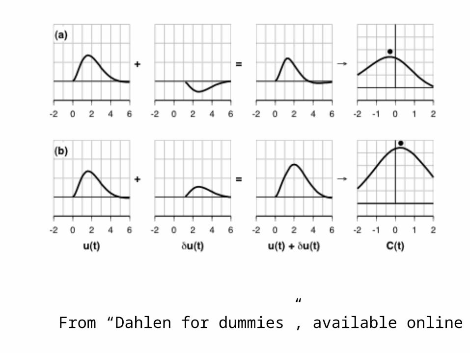
From “Dahlen for dummies”, available online

Banana-Donut kernels

• Requires:– Good first guess at
model
– Good constraints on source size, location
– Big computers
• Results in:– More accurate models of
mantle structure
– More precise models, including better resolution of potential plumes/slabs (Montelli found many more plumes!)
P
PP

D’’
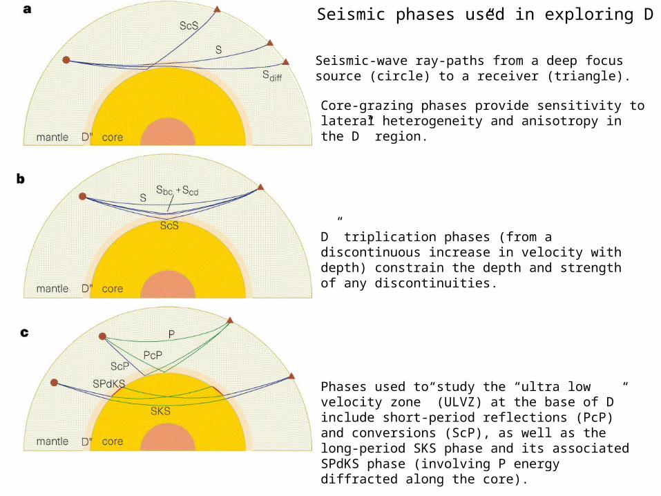
Seismic phases used in exploring D”
Seismic-wave ray-paths from a deep focus source (circle) to a receiver (triangle).
Core-grazing phases provide sensitivity to lateral heterogeneity and anisotropy in the D” region.
D” triplication phases (from a discontinuous increase in velocity with depth) constrain the depth and strength of any discontinuities.
Phases used to study the “ultra low velocity zone” (ULVZ) at the base of D” include short-period reflections (PcP) and conversions (ScP), as well as the long-period SKS phase and its associated SPdKS phase (involving P energy diffracted along the core).

Alaska and the Caribbean
•Abrupt increase in Vs
•Negative gradients in D’’
•Relatively cold in D’’
•Shear wave splitting at top of discontinuity (shown as fluctuations, may be caused by melt)
•No ultra low velocity zone (ULVZ)
Central Pacific region
•No strong discontinuity, but neg. gradient
•Relatively hot in D’’
•Thick, pronounced ULVZ (5-30% decrease)
•Laterally variable anisotropy close to base (fluctuations)
The main classes of D" shear-wave velocity structures.
Schematic shear-wave velocity structures, shown as per cent deviations (VS)

Spatial patterns of seismological characteristics of the CMB boundary layer
a, Regions with detectable ultra-low-velocity zone (ULVZ) in red, and sampled regions that lack evidence of any ULVZ are shown in blue.
b, Regions with shear-wave anisotropy in D” are shown.

The chemical heterogeneities schematically shown here could be due to:Partial meltingcore–mantle reaction products, slab-associated geochemical heterogeneities

Attenuation of seismic waves
From: Myers et al.
•Some materials (e.g., hot and/or with lots of fluids) dampen seismic waves more than others
• Seismic waves from South America felt more strongly in Canada than in Salt Lake City
• Example from South America
Key: Independent evidence, complementary to observed P and S wave travel times

Global maps of attenuation
•At shallow depths, similar to velocity maps: low velocities and attenuation beneath ridges; high values below continents
•Evidence for super plume beneath south Pacific
• Very difficult to resolve small scale structures like individual plumes
Depends on many things, including heat flow…..
From:Romanowicz and Gung, 2002

Global Heat Flow
From: Pollack et al., 1993
•Highs at Mid-ocean ridges
•Lows mostly over continentsThink: convection heat vs. radiogenic heat?
• Compare with solar radiation:~1400 W/m^2, top of atmosphere
• Total terrestrial heat fluxaverage: 0.087 W/m^2
• Total Power ~40 TW

Measuring heat flow
• Simple equation, hard to measure
• Need: T/x
– T at two depths– But…
• Hole disturbs T• May have to wait a
long time• Local effects,
advection?• Topography?
K = thermal conductivityA=areaT/x = temp gradient
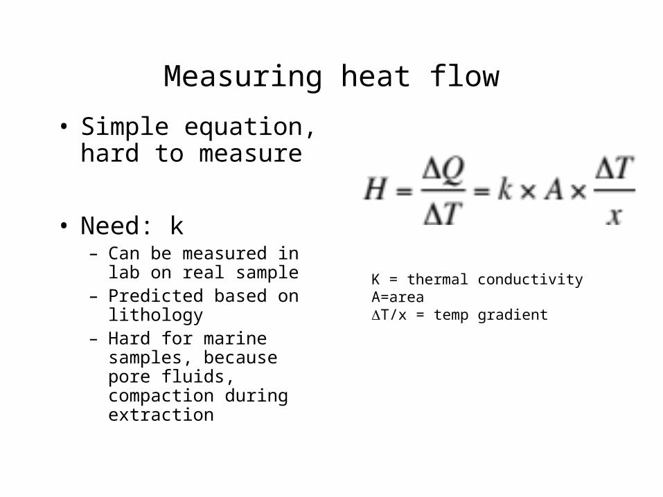
Measuring heat flow
• Simple equation, hard to measure
• Need: k– Can be measured in lab
on real sample– Predicted based on
lithology– Hard for marine samples,
because pore fluids, compaction during extraction
K = thermal conductivityA=areaT/x = temp gradient

• Goal: steady-state heat flow• Problems:
– Seasonal/daily• T gradient depends on surface temperature too• T cycles penetrate to various depths, w/ various
magnitudes• (take geodynamics)
– Rapid sedimentation or erosion• If dT/dz is perturbed completely within the region
sampled, estimates of heat flow will be biased
Measuring heat flow
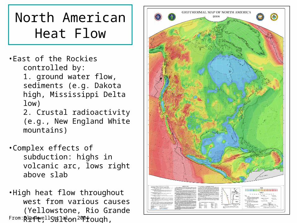
North American Heat Flow
From:Blackwell et al., 2004
•East of the Rockies controlled by:1. ground water flow, sediments (e.g. Dakota high, Mississippi Delta low)2. Crustal radioactivity (e.g., New England White mountains)
•Complex effects of subduction: highs in volcanic arc, lows right above slab
•High heat flow throughout west from various causes (Yellowstone, Rio Grande Rift, Salton Trough, Basin and Range)