Steffen HölldoblerYanchun Liang(Eds.)

1st International Workshop onSemantic Technologies(IWOST)

Proceedings

March 9–12 2015

Jilin University, Changchun, China

Volume Editors

Steffen HölldoblerInternational Center for Computational LogicTechnische Universität Dresden01062 Dresden, Germanyemail: sh@iccl.tu-dresden.de

Yanchun LiangJilin UniversityChangchun, ChinaEmail: ycliang@jlu.edu.cn

Copyright c© 2015 for the individual papers by the papers’ authors. Copyingpermitted only for private and academic purposes. This volume is published andcopyrighted by its editors.

3

Preface

This volume contains the papers presented at the First International Workshopon Semantic Technologies (IWOST) held on March 09-12, 2015 at the Jilin Uni-versity in Changchun, China. The workshop is an activity of the cluster SemanticTechnologies with the project Swap and Transfer. This project is funded by theEU within the Erasmus Mundus programme and aims at fostering sustainabledevelopment, innovation and technology transfer.

There were 14 submissions. Each submission was reviewed by at least 2 programcommittee members. The committee decided to accept 11 papers. The programalso includes invited talks by Fausto Guinchiglia from the University of Trento onOpen Data Integration, Cleaning and Reuse and by Chagnaa Altangerel from theNational University of Mongolia on Language Resources in the Semantic Web.

The editors would like to thank Peter Steinke for his help in setting up the webpage and compiling this proceedings as well as the local organizers at Jilin Uni-versity without which the workshop would not have been possible. We thank theSwap and Transfer project as well as Jilin University for supporting the workshopfinancially. Finally, we are indepted to Easy Chair which made the organizationof the workshop easy for the chairs.

March 6, 2015Dresden and Changchun

Steffen HölldoblerYanchun Liang

4

Program Committee

Idilia Bachkova Chimikotehnologitchen I Metalurgitchen UniversitetKhang Tran Dinh Hanoi University of Science and TechnologyAnna Fensel University of InnsbruckSteffen Hölldobler Technische Universitaet DresdenYanchun Liang University of JilinMaurizio Marchese University of TrentoThai Ha Phi Hanoi University of Transport and CommunicationSrun Sovila Royal University of Phnom PhenHao Xu University of Jilin

Additional Reviewers

Norbert MantheyTobias Philipp

5

Contents

Minglinag Cui, Yanchun Liang, Yuping Li and Renchu GuanExploring Trends of Cancer Research Based on Topic Model . . . . . . . . . . . 7

Emmanuelle Anna Dietz, Steffen Hölldobler and Luís MonizPereiraOn Indicative Conditionals . . . . . . . . . . . . . . . . . . . . . . . . . . . . . . . . . . . . . . . . . . . . 19

Shasha Feng, Michel Ludwig and Dirk WaltherThe Logical Difference for EL: from Terminologies towards TBoxes . . . . 31

Anna Fensel, Elias Kärle and Ioan TomaTourPack: Packaging and Disseminating Touristic Services withLinked Data and Semantics . . . . . . . . . . . . . . . . . . . . . . . . . . . . . . . . . . . . . . . . . . . . 43

Lei Liu, Quanzhu Tao, Fausto Giunchiglia and Rui ZhangA Practical Framework for RelBAC Implementation . . . . . . . . . . . . . . . . . . . 55

Ji Qingge and Han YugangNovel Integrated Framework for Crowd Simulation . . . . . . . . . . . . . . . . . . . . . 67

Adriano Tavares, Fausto Giunchiglia, Hao Xu and Yanchun LiangPosition on Interoperability Everywhere under IoT-ARM . . . . . . . . . . . . . . 79

Hai Van Pham and Khang Dinh TranA Proposal of Model using Kansei Evaluation Integrated withFuzzy Rules and Self-Organizing Map for Evaluation ofBio-Food Products . . . . . . . . . . . . . . . . . . . . . . . . . . . . . . . . . . . . . . . . . . . . . . . . . . . . . 85

Yiyuan Wang, Dantong Ouyang and Liming ZhangImproved algorithm of unsatisfiability-based Maximum Satisfiability . . . . 93

Yuxin Ye and Dantong OuyangEntailment-based Axiom Pinpointing in Debugging IncoherentTerminologies . . . . . . . . . . . . . . . . . . . . . . . . . . . . . . . . . . . . . . . . . . . . . . . . . . . . . . . . . 105

Yu Zhang, Dantong Ouyang and Yuxin YeAn Automatic Way of Generating Incoherent Terminologies withParameters . . . . . . . . . . . . . . . . . . . . . . . . . . . . . . . . . . . . . . . . . . . . . . . . . . . . . . . . . . . . 117

Exploring Trends of Cancer Research Based on Topic Model

Mingliang Cui, Yanchun Liang*, Yuping Li, Renchu Guan* College of Computer Science and Technology, Jilin University,

Changchun, 130012, China {Yanchun Liang ycliang@jlu.edu.cn; Renchu Guan guanrenchu@jlu.edu.cn}

Abstract. Cancer research is of great importance in life science and medicine and attracts research funds of thousands of millions dollars each year. With the explosion of biomedical research papers, it becomes more and more necessary to show the research trend in this spotlight area. In this paper, to provide a straightforward research atlas for the top killer cancers, Latent Dirichlet Allocation (LDA) is performed on the massive quantities of biomedical literatures. Moreover, Gibbs Sampling is used to make assessment on the parameters of the LDA model. The proposed evaluation carried out under multiple conditions with different Ks (the number of topics) for the top five cancers in recent five years. Additionally, a biomedical topic model was generated with the LDA model and delicate analysis was performed on the basis of that in order to explore the trending topic in cancer research. It can help the biology and medicine doctors quickly catch the frontiers of the cancer study, improve and expand their research programme, especially in today’s era of “big data”. Key words: Topic Model, LDA, Gibbs Sampling, Topic Analysis, Cancer Research Trend

1 Introduction

1.1 Significance

Cancer is of great threat to human health, scientists and Medicians have been continuously looking for effective treatment to conquer it, however, cancer research is a very challenging field in today's life science. Over the past 5 years cancer research has diverged enormously, partly based on the quickly development of biotechnology and bioinformatics. It is not easy to summarize recent trends for different cancers’ study, and identify where the new findings are and therapies might come from [1]. Under this circumstance, we choose an appropriate machine learning method―topic model―to explore the trend in cancer research, specifically, the topics in cancer research papers.

The topic model is a probabilistic model of text mining appeared in recent years [2]. It is an algorithm that can discover the topic structure hidden in large-scale data. In topic model, the vocabulary items is visible while the topic structure hidden. In order

to reduce the dimensions of the feature vector space, texts are usually mapped into the topic space via the topic model. It is different from the traditional vector space model, which just simply considers each document as a sample and each word as a feature. Instead, it maps a high dimensional frequency space to a lower dimensional topic space. Moreover, the topic model can capture the semantic information, which can reveal that the latent relations among documents. It also can effectively solve the polysemy, synonym and other problems, which has the vital significance in document feature extraction and content analysis. However, using a topic model (i.e. Latent Dirichlet Allocation) to analyze the trends of cancers has not been reported.

The rest of the article is organized as follows: we start in section 2 with a brief review of a topic model named as Latent Dirichlet Allocation and its related work. In section 3, the algorithm of Gibbs Sampling is introduced, and the framework of our exploration is described in detail. It presents the experimental methodology and results on Medline dataset in Section 4. At last, conclusions and future work are depicted in Section 5.

2 Background

In 1998, Professor Papadimitriou proposes LSI (Latent Semantic Indexing) model [3], which can be seen as the origin of the Topic model. In 1999, Professor Hofmann put it forward to pLSI (Probabilistic Latent Semantic Indexing) model [4] and LDA (Latent Dirichlet Allocation) is a generalization of pLSI, which adds Dirichlet Bias generating prior distribution model, proposed by Blei in 2003[5].

LDA has been widely applied in information retrieval, text mining, Natural Language Processing fields and has become a research hotspots recently [6-8]. In this paper, LDA model is introduced to analyze the Medline data especially on cancer research. In the LDA model, a document is generated as follows [9]:

1. First, generate the topic distribution of the document i by sampling from the dirichlet distribution .

2. Second, generate the topic of the word j in the document i by sampling from the topic distribution.

3. Then generate the word distribution of the topic by sampling from the Dirichlet distribution .

4. Finally generate the word j in the document i by sampling from the word distribution.

Which is similar to the binomial distribution Beta distribution [10] is the conjugate prior probability distribution [11], while the Dirichlet distribution is a polynomial distributed conjugate prior probability distribution.

The structure diagram of LDA model is shown in the Figure.1 (similar to the Bayesian network structure [12]):

8

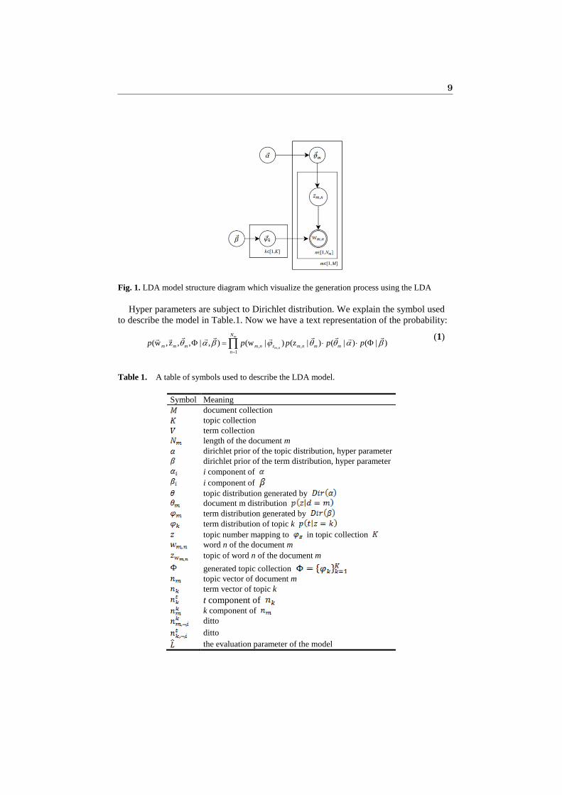
Fig. 1. LDA model structure diagram which visualize the generation process using the LDA

Hyper parameters are subject to Dirichlet distribution. We explain the symbol used to describe the model in Table.1. Now we have a text representation of the probability:

,, ,1

(w , z , , ) (w | ) (z || , ) ( ( )|| )m

m n

N

m m m m n z m n m mn

p p p p pθ ϕ θα β θ βα=

Φ Φ= ⋅ ⋅∏ (1)

Table 1. A table of symbols used to describe the LDA model.

Symbol Meaning document collection topic collection

term collection length of the document m

dirichlet prior of the topic distribution, hyper parameter dirichlet prior of the term distribution, hyper parameter i component of i component of

topic distribution generated by document m distribution term distribution generated by term distribution of topic k

topic number mapping to in topic collection word n of the document m

topic of word n of the document m

generated topic collection topic vector of document m

term vector of topic k t component of k component of

ditto

ditto the evaluation parameter of the model

9

The convergence of LDA is a more critical issue. We use the convergence function to solve it. Under the given model conditions, we choose the appearance probability of samples as the evaluation criterion of the model. The performance of the LDA model:

1

(w | M) (w | , )M

m mm

p p θ=

Φ=∏ (2)

11 1

1 1

( )m t kNM K

k t m kV Kt k

km n k t m kt k

n nn nβ αβ α== =

= =

+ += ⋅

+ +∑∏∏∑ ∑

. (3)

For the convenience of the calculation, we use log transform to the equation (1), denoted as . Along with the iterative constantly, is used to determine the model convergence [13].

21

1 11 1

ˆ= - (l ( ))ogm t k

k t m kV Kt k

NM K

m k t m kt kn k

n nLn nβ αβ α= =

= ==

+ +⋅

+ +∑

∑∑

∑∑ (4)

3 Main Work

3.1 Core Method

In fact, LDA is one of the probabilistic. Data are generally divided into two parts, visible variables and latent variables. It is believed in the topic model that the data is produced by the generation process, which defines the joint probability distribution of visible random variables and latent random variables. For many modern probabilistic models, including Bayesian statistics, the priori probability calculation is extremely difficult. So the core research objective of modern probability modelling is to do everything possible to obtain an approximate solution. Random sampling is a kind of methods for solving the approximate solution with good performance. This article describes a method commonly used sampling MCMC (Markov Chain Monte Carlo) [14] and Gibbs Sampling algorithm [15], Gibbs Sampling algorithm has been widely used in modern Bayesian analysis.

MCMC methods have Gibbs Sampling algorithm and Metropolis-Hastings (MH) [16] algorithm commonly used sampling methods. Gibbs Sampling algorithm is a special case of MH algorithm, Gibbs Sampling from a high-dimensional space are sampled separately for each dimension, and gradually get higher dimensional sampling points, making sampling difficult to reduce.

N-dimensional Gibbs Sampling: 1. Random initialization { : 1, 2, ,ix i n= ⋅⋅⋅ }

2. For 0,1,2,t = ⋅⋅⋅ loop in sampling )1(

1+tx ～ 1 2 3(x | x , x , , x )t t t

np ⋅ ⋅ ⋅

10

… )1( +t

jx ～ (t 1) (t 1)1 1 1(x | x , , x , x , , x )t t

j j j np + +− +⋅⋅ ⋅ ⋅ ⋅ ⋅

… )1( +t

nx ～ ),,,|( 11

12

11

+−

++ ⋅⋅⋅ tn

ttn xxxxp

3.2 Complete Process

We choose the top 5 cancer from the top 10 deadliest cancer published by the LiveScience [17], which are Breast Cancer, Lung Cancer, Pancreatic Cancer, Prostate Cancer and Colon Cancer. We search and download the research paper related to these cancers from NCBI PubMed from 2010 to 2014 separately [18].

Then we make a pre-process to extract the title and abstract for each paper and make some hyphens for the entity name for a better segmentation. After that we use WordNet [19] to stem the text in order to get an exact description for the topic. Before the document input into model, we will do the pre-processing for the document, thereby obtaining the document term matrix. It can be seen by term matrix that how many documents in corpus, how many word terms and how frequently each term appears in a document. The inputs of the model are the document collection , the number of topics , and the hyper parameters .The topic of a number K we need to specify its value according to the experience, we want to take advantages of K solution, the need for repeated experiments, and then to carry on the value according to the different K value under the situation of convergence. After repeated experiments of LDA convergence on the data, we get a reasonable value of K=100. The hyper parameter is the Dirichlet of the prior distribution. In fact they have smooth effect on data. Because there is no supervision information too much, we assign the hyper parameters an empirical value , , tending to take symmetry value [20].

Take the dataset of Pancreatic Cancer in 2010 as an example, the number of the abstract is 2088, includes 54004 words. The number of topic K is set to 100, 200, 300, 400, 500, considered for model convergence condition.

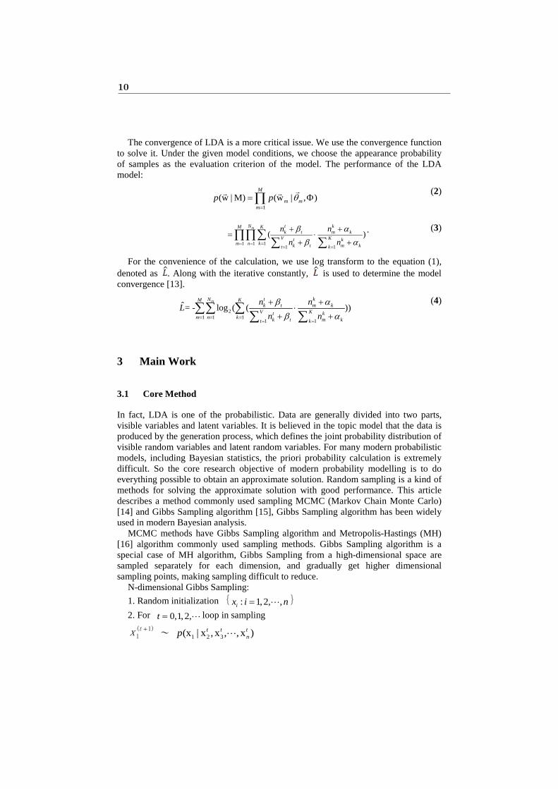
According to the evaluation function of the convergence mentioned in Section 2, which shows the cost of compression of the text using the model, the smaller the better. Figure.2 below respectively under different K values for the iterative convergence condition of iteration times of 400 and 1000.

11

Fig. 2. The 400 iteration convergence condition of the LDA Gibbs Sampling model. X-axis is iterations, Y-axis is results of convergence function.

We further analysis the output of the LDA Gibbs Sampling, particularly in the topic words file (this file contains topic words most likely words of each topic). We first transform the topic-word matrix to a topic word vector representing the selection and the frequency of topic words to describe one cancer research. Then we use feature scaling normalization [21] (formula 5) to deal with the word vector, in order to compare them between different years and different cancers.

(5)

We measure the similarity and differences between the 5 cancer research by their word vector cosine coefficients similarity [22] (formula 6).

(6)

Unlike the cosine coefficients which give a numerical description on the trend and topic of the 5 cancers, the common words are easier for readers to have an intuition on the 5 cancers topics. We do the both analysis of the results so that we may get a comprehensive answer.

4 Experiments and Discussion

To examine the behavior and the performance of LDA, the experiments are illustrated on the widely used Medline dataset. In order to straightforwardly compare the trend and topic resulted from the LDA model, the visual results to get the entire recognition of the topic words of different cancers are shown, which uses the Word Cloud tool supported by Tagul.com [24]. And we also draw the trend of cancer research in different years, supported by Plot.ly [25].

12

4.1 Experimental Setup

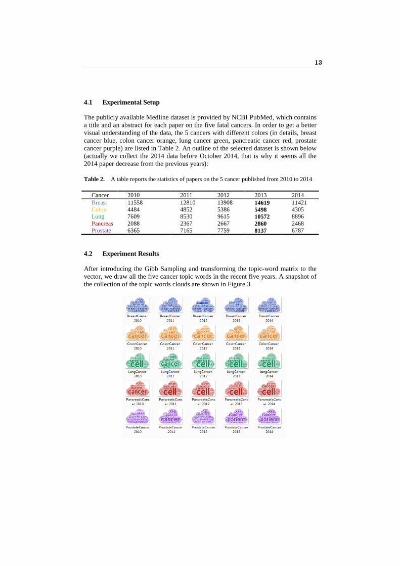
The publicly available Medline dataset is provided by NCBI PubMed, which contains a title and an abstract for each paper on the five fatal cancers. In order to get a better visual understanding of the data, the 5 cancers with different colors (in details, breast cancer blue, colon cancer orange, lung cancer green, pancreatic cancer red, prostate cancer purple) are listed in Table 2. An outline of the selected dataset is shown below (actually we collect the 2014 data before October 2014, that is why it seems all the 2014 paper decrease from the previous years):

Table 2. A table reports the statistics of papers on the 5 cancer published from 2010 to 2014

Cancer 2010 2011 2012 2013 2014 Breast 11558 12810 13908 14619 11421 Colon 4484 4852 5386 5498 4305 Lung 7609 8530 9615 10572 8896 Pancreas 2088 2367 2667 2860 2468 Prostate 6365 7165 7759 8137 6787

4.2 Experiment Results

After introducing the Gibb Sampling and transforming the topic-word matrix to the vector, we draw all the five cancer topic words in the recent five years. A snapshot of the collection of the topic words clouds are shown in Figure.3.

13

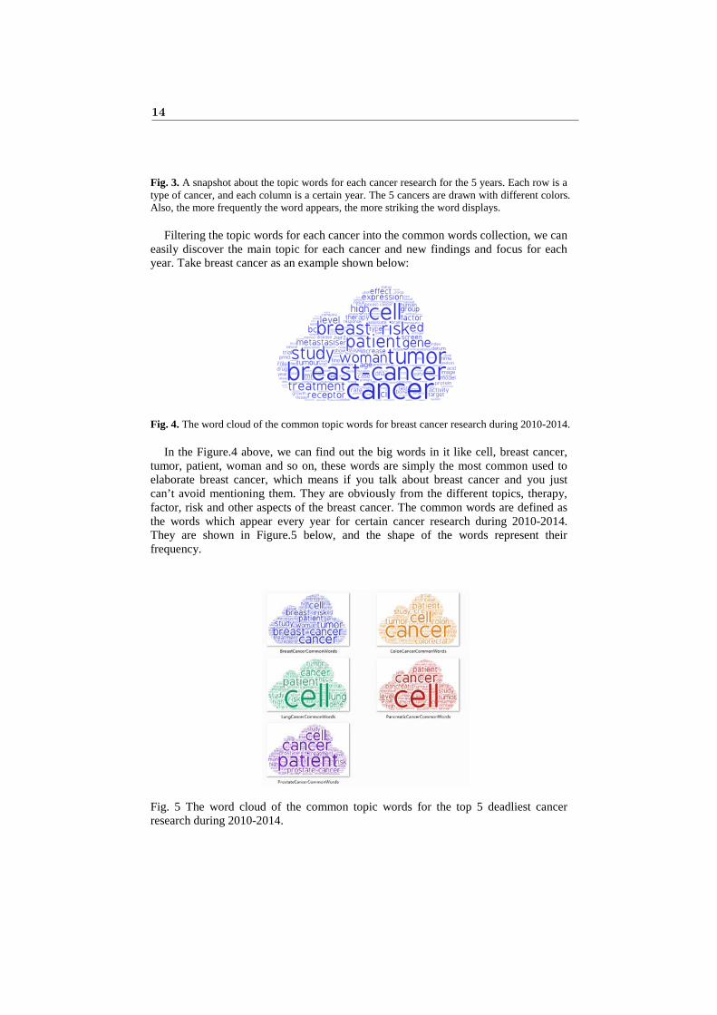
Fig. 3. A snapshot about the topic words for each cancer research for the 5 years. Each row is a type of cancer, and each column is a certain year. The 5 cancers are drawn with different colors. Also, the more frequently the word appears, the more striking the word displays.

Filtering the topic words for each cancer into the common words collection, we can easily discover the main topic for each cancer and new findings and focus for each year. Take breast cancer as an example shown below:

Fig. 4. The word cloud of the common topic words for breast cancer research during 2010-2014.

In the Figure.4 above, we can find out the big words in it like cell, breast cancer, tumor, patient, woman and so on, these words are simply the most common used to elaborate breast cancer, which means if you talk about breast cancer and you just can’t avoid mentioning them. They are obviously from the different topics, therapy, factor, risk and other aspects of the breast cancer. The common words are defined as the words which appear every year for certain cancer research during 2010-2014. They are shown in Figure.5 below, and the shape of the words represent their frequency.

Fig. 5 The word cloud of the common topic words for the top 5 deadliest cancer research during 2010-2014.

14

4.3 General Comparison and Discussions

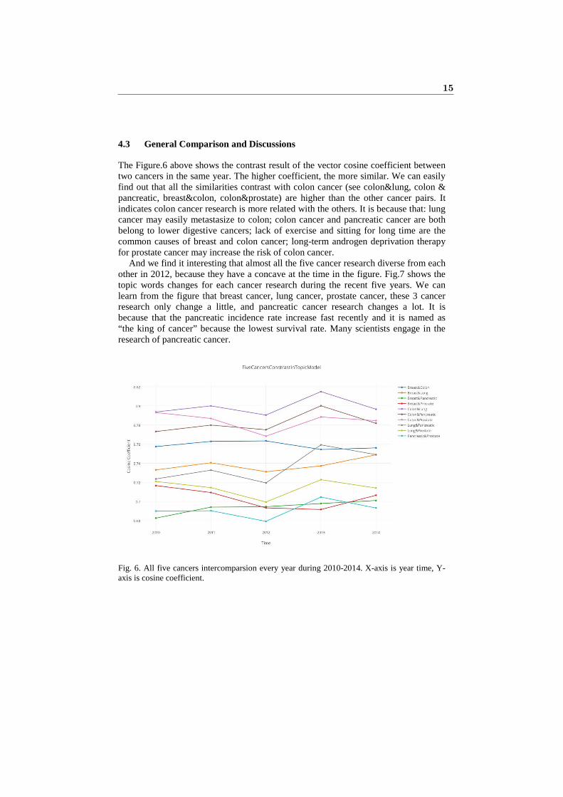
The Figure.6 above shows the contrast result of the vector cosine coefficient between two cancers in the same year. The higher coefficient, the more similar. We can easily find out that all the similarities contrast with colon cancer (see colon&lung, colon & pancreatic, breast&colon, colon&prostate) are higher than the other cancer pairs. It indicates colon cancer research is more related with the others. It is because that: lung cancer may easily metastasize to colon; colon cancer and pancreatic cancer are both belong to lower digestive cancers; lack of exercise and sitting for long time are the common causes of breast and colon cancer; long-term androgen deprivation therapy for prostate cancer may increase the risk of colon cancer.

And we find it interesting that almost all the five cancer research diverse from each other in 2012, because they have a concave at the time in the figure. Fig.7 shows the topic words changes for each cancer research during the recent five years. We can learn from the figure that breast cancer, lung cancer, prostate cancer, these 3 cancer research only change a little, and pancreatic cancer research changes a lot. It is because that the pancreatic incidence rate increase fast recently and it is named as “the king of cancer” because the lowest survival rate. Many scientists engage in the research of pancreatic cancer.

Fig. 6. All five cancers intercomparsion every year during 2010-2014. X-axis is year time, Y-axis is cosine coefficient.

15

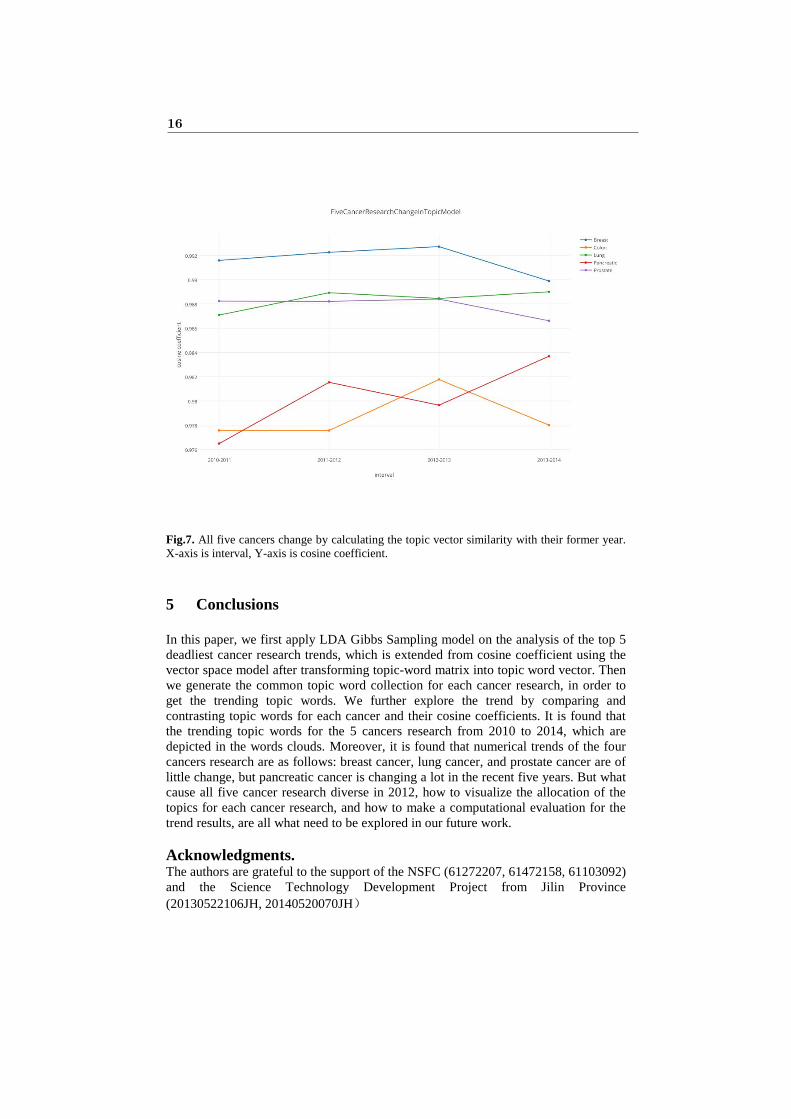
Fig.7. All five cancers change by calculating the topic vector similarity with their former year. X-axis is interval, Y-axis is cosine coefficient.

5 Conclusions

In this paper, we first apply LDA Gibbs Sampling model on the analysis of the top 5 deadliest cancer research trends, which is extended from cosine coefficient using the vector space model after transforming topic-word matrix into topic word vector. Then we generate the common topic word collection for each cancer research, in order to get the trending topic words. We further explore the trend by comparing and contrasting topic words for each cancer and their cosine coefficients. It is found that the trending topic words for the 5 cancers research from 2010 to 2014, which are depicted in the words clouds. Moreover, it is found that numerical trends of the four cancers research are as follows: breast cancer, lung cancer, and prostate cancer are of little change, but pancreatic cancer is changing a lot in the recent five years. But what cause all five cancer research diverse in 2012, how to visualize the allocation of the topics for each cancer research, and how to make a computational evaluation for the trend results, are all what need to be explored in our future work.

Acknowledgments. The authors are grateful to the support of the NSFC (61272207, 61472158, 61103092) and the Science Technology Development Project from Jilin Province (20130522106JH, 20140520070JH）

16

References

1. Cao, Y., DePinho, R., Ernst, M., Vousden, K.: Cancer research: past, present and future. Nature Reviews Cancer. 11, 749–754 (2011).

2. Rosen-Zvi, M., Griffiths, T., Steyvers, M., & Smyth, P.: The author-topic model for authors and documents. Proceedings of the 20th conference on Uncertainty in artificial intelligence. 487-494 (2004).

3. Papadimitriou, C. H., Tamaki, H., Raghavan, P., & Vempala, S.: Latent semantic indexing: A probabilistic analysis. Proceedings of the seventeenth ACM SIGACT-SIGMOD-SIGART symposium on Principles of database systems. 159-168 (1998).

4. Hofmann, T.: Probabilistic latent semantic indexing. Proceedings of the 22nd annual international ACM SIGIR conference on Research and development in information retrieval. 50-57 (1999).

5. Blei, D. M., Ng, A. Y., & Jordan, M. I.: Latent dirichlet allocation. the Journal of machine Learning research, 3, 993-1022 (2003).

6. Teh, Y. W., Jordan, M. I., Beal, M. J., & Blei, D. M.: Hierarchical dirichlet processes. Journal of the american statistical association 101.476 (2006).

7. Mcauliffe, Jon D., David M. Blei.: Supervised topic models. Advances in neural information processing systems. 121-128 (2008).

8. Petinot, Yves, Kathleen McKeown, and Kapil Thadani.: A hierarchical model of web summaries. In: Proceedings of the 49th Annual Meeting of the Association for Computational Linguistics: Human Language Technologies: short papers-Volume 2. 670-675. Association for Computational Linguistics (2011).

9. Diebolt, Jean, Christian P. Robert.: Estimation of finite mixture distributions through Bayesian sampling. Journal of the Royal Statistical Society. Series B (Methodological). 363-375 (1994).

10. S. Kotz, N. Balakrishnan, N. L. Johnson: Dirichlet and Inverted Dirichlet Distributions. Continuous Multivariate Distributions, Models and Applications. New York: Wiley, 2000., United States (2004).

11. Lindley, Dennis V.: The use of prior probability distributions in statistical inference and decision. Proc. 4th Berkeley Symp. on Math. Stat. and Prob. 453-468 (1961).

12. Beal, Matthew James.: Variational algorithms for approximate Bayesian inference. PhD diss. University of London (2003).

13. Heinrich, Gregor.: Parameter estimation for text analysis. Technical report. (2005). 14. Gilks, Walter R.: Markov chain monte carlo. John Wiley & Sons, Ltd. (2005). 15. Porteous, Ian, David Newman, Alexander Ihler, Arthur Asuncion, Padhraic Smyth, Max

Welling.: Fast collapsed gibbs sampling for latent dirichlet allocation. Proceedings of the 14th ACM SIGKDD international conference on Knowledge discovery and data mining. 569-577 (2008).

16. Chib S., Greenberg E.: Understanding the metropolis-hastings algorithm. The american statistician. 49(4): 327-335 (1995).

17

17. Chan, A.: The 10 Deadliest Cancers and Why There’s No Cure, http://www.livescience.com/11041-10-deadliest-cancers-cure.html.

18. Ncbi.nlm.nih.gov,: Home - PubMed - NCBI, http://www.ncbi.nlm.nih.gov/pubmed. 19. University, P.: About WordNet - WordNet - About WordNet, http://wordnet.princeton.edu/. 20. Griffiths, T., Steyvers: Finding scientific topics. Proceedings of the National Academy of

Sciences. 101, 5228–5235 (2004). 21. Wikipedia,: Normalization, http://en.wikipedia.org/wiki/Normalization. 22. Wikipedia,: Cosine similarity, http://en.wikipedia.org/wiki/Cosine_similarity. 23. O'Rourke, Norm, R. Psych, Larry Hatcher.: A step-by-step approach to using SAS for

factor analysis and structural equation modeling. Sas Institute. (2013). 24. Tagul.com,: Tagul - Gorgeous word clouds, http://tagul.com. 25. Plot.ly,: Plotly, https://plot.ly/.

18

On Indicative Conditionals

Emmanuelle Anna Dietz1, Steffen Holldobler1, and Luıs Moniz Pereira2?

1International Center for Computational Logic, TU Dresden, Germany,{dietz,sh}@iccl.tu-dresden.de

2NOVA Laboratory for Computer Science and Informatics, Caparica, Portugal,lmp@fct.unl.pt

Abstract. In this paper we present a new approach to evaluate indica-tive conditionals with respect to some background information specifiedby a logic program. Because the weak completion of a logic program ad-mits a least model under the three-valued Lukasiewicz semantics and thissemantics has been successfully applied to other human reasoning tasks,conditionals are evaluated under these least L-models. If such a modelmaps the condition of a conditional to unknown, then abduction andrevision are applied in order to satisfy the condition. Different strategiesin applying abduction and revision might lead to different evaluations ofa given conditional. Based on these findings we outline an experiment tobetter understand how humans handle those cases.

1 Indicative Conditionals

Conditionals are statements of the form if condition then consequence. In theliterature the condition is also called if part, if clause or protasis, whereas theconsequence is called then part, then clause or apodosis. Conditions as well asconsequences are assumed to be finite sets (or conjunctions) of ground literals.

Indicative conditionals are conditionals whose condition may or may not betrue and, consequently, whose consequence also may or may not be true; however,the consequence is asserted to be true if the condition is true. Examples forindicative conditionals are the following:

If it is raining, then he is inside. (1)

If Kennedy is dead and Oswald did not shoot him, then someone else did. (2)

If rifleman A did not shoot, then the prisoner is alive. (3)

If the prisoner is alive, then the captain did not signal. (4)

If rifleman A shot, then rifleman B shot as well. (5)

If the captain gave no signal and rifleman A decides to shoot,

then the prisoner will die and rifleman B will not shoot. (6)

Conditionals may or may not be true in a given scenario. For example, if weare told that a particular person is living in a prison cell, then most people are

? The authors are mentioned in alphabetical order.

expected to consider (1) to be true, whereas if we are told that he is living inthe forest, then most people are expected to consider (1) to be false. Likewise,most people consider (2) to be true.

The question which we shall be discussing in this paper is how to automatereasoning such that conditionals are evaluated by an automated deduction sys-tem like humans do. This will be done in a context of logic programming (cf.[11]), abduction [9], Stenning and van Lambalgen’s representation of condition-als as well as their semantic operator [19] and three-valued Lukasiewicz logic[12], which has been put together in [6,7,5,8,3] and has been applied to the sup-pression [2] and the selection task [1], as well as to model the belief-bias effect[15] and contextual abductive reasoning with side-effects [16].

The methodology of the approach presented in this paper differs significantlyfrom methods and techniques applied in well-known approaches to evaluate(mostly subjunctive) conditionals like Ramsey’s belief-retention approach [17],Lewis’s maximal world-similarity one [10], Rescher’s systematic reconstructionof the belief system using principles of saliency and prioritization [18], Ginsberg’spossible worlds approach [4] and Pereira and Aparıco’s improvements thereof byrequiring relevancy [14]. Our approach is inspired by Pearl’s do-calculus [13] inthat it allows revisions to satisfy conditions whose truth-value is unknown andwhich cannot be explained by abduction, but which are amenable to hypotheticalintervention instead.

2 Preliminaries

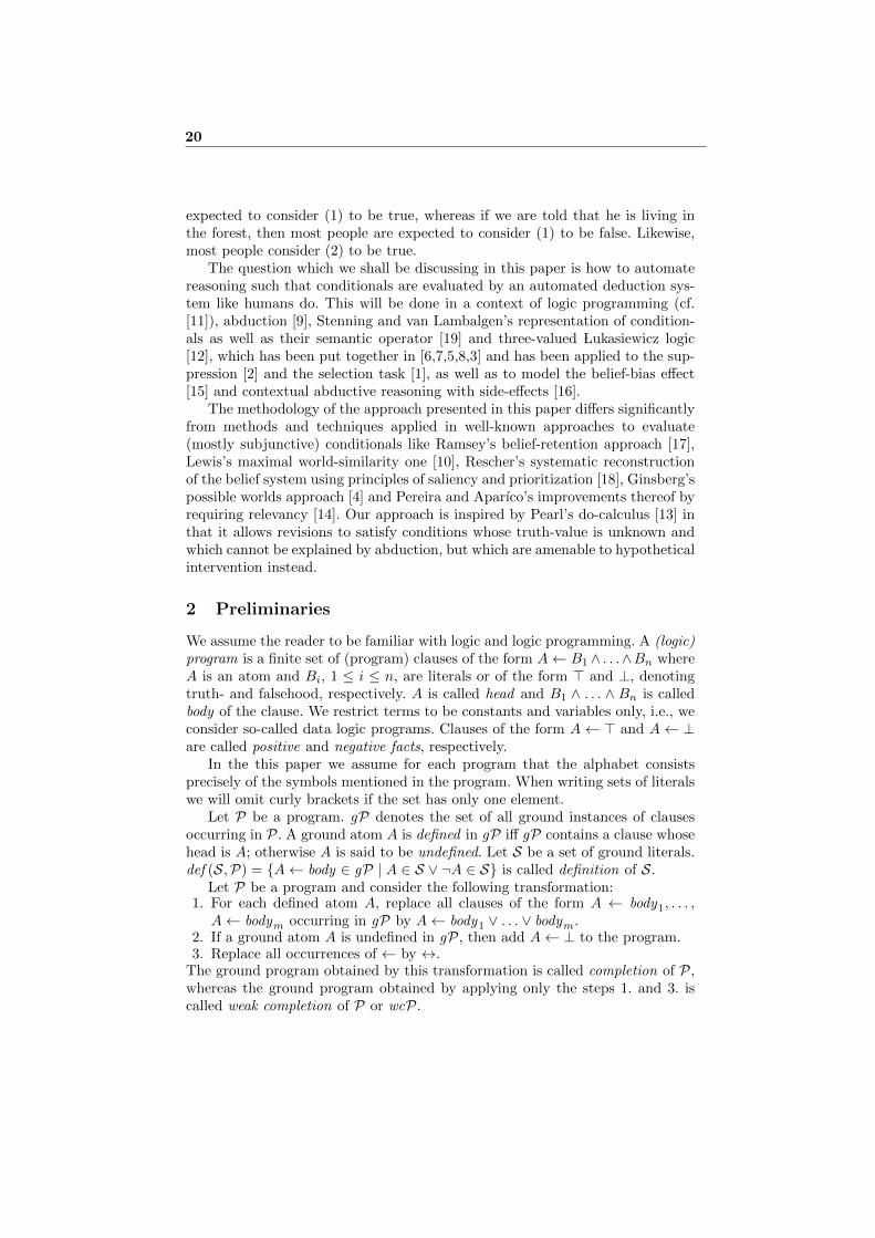
We assume the reader to be familiar with logic and logic programming. A (logic)program is a finite set of (program) clauses of the form A← B1∧ . . .∧Bn whereA is an atom and Bi, 1 ≤ i ≤ n, are literals or of the form > and ⊥, denotingtruth- and falsehood, respectively. A is called head and B1 ∧ . . . ∧ Bn is calledbody of the clause. We restrict terms to be constants and variables only, i.e., weconsider so-called data logic programs. Clauses of the form A← > and A← ⊥are called positive and negative facts, respectively.

In the this paper we assume for each program that the alphabet consistsprecisely of the symbols mentioned in the program. When writing sets of literalswe will omit curly brackets if the set has only one element.

Let P be a program. gP denotes the set of all ground instances of clausesoccurring in P. A ground atom A is defined in gP iff gP contains a clause whosehead is A; otherwise A is said to be undefined. Let S be a set of ground literals.def (S,P) = {A← body ∈ gP | A ∈ S ∨ ¬A ∈ S} is called definition of S.

Let P be a program and consider the following transformation:1. For each defined atom A, replace all clauses of the form A ← body1, . . . ,A← bodym occurring in gP by A← body1 ∨ . . . ∨ bodym.

2. If a ground atom A is undefined in gP, then add A← ⊥ to the program.3. Replace all occurrences of ← by ↔.

The ground program obtained by this transformation is called completion of P,whereas the ground program obtained by applying only the steps 1. and 3. iscalled weak completion of P or wcP.

20

We consider the three-valued Lukasiewicz (or L-) semantics [12] and representeach interpretation I by a pair 〈I>, I⊥〉, where I> contains all atoms which aremapped to true by I, I⊥ contains all atoms which are mapped to false by I, andI> ∩ I⊥ = ∅. Atoms occurring neither in I> not in I⊥ are mapped to unknown.Let 〈I>, I⊥〉 and 〈J>, J⊥〉 be two interpretations. We define

〈I>, I⊥〉 ⊆ 〈J>, J⊥〉 iff I> ⊆ J> and I⊥ ⊆ J⊥.

Under L-semantics we find F ∧ > ≡ F ∨ ⊥ ≡ F for each formula F , where ≡denotes logical equivalence. Hence, occurrences of the symbols > and ⊥ in thebodies of clauses can be restricted to those occurring in facts.

It has been shown in [6] that logic programs as well as their weak completionsadmit a least model under L-semantics. Moreover, the least L-model of the weakcompletion of P can be obtained as least fixed point of the following semanticoperator, which was introduced in [19]: ΦP(〈I>, I⊥〉) = 〈J>, J⊥〉, where

J> = {A | A← body ∈ gP and body is true under 〈I>, I⊥〉},J⊥ = {A | def (A,P) 6= ∅ and

body is false under 〈I>, I⊥〉 for all A← body ∈ def (A,P)}.

We define P |=lmwc L F iff formula F holds in the least L-model of wcP.

As shown in [2], the L-semantics is related to the well-founded semanticsas follows: Let P be a program which does not contain a positive loop and letP+ = P \ {A ← ⊥ | A ← ⊥ ∈ P}. Let u be a new nullary relation symbol notoccurring in P and B be a ground atom in

P∗ = P+ ∪ {B ← u | def (B,P) = ∅} ∪ {u← ¬u}.

Then, the least L-model of wcP and the well-founded model for P∗ coincide.An abductive framework consists of a logic program P, a set of abducibles

AP = {A← > | A is undefined in gP} ∪ {A← ⊥ | A is undefined in gP}, a setof integrity constraints IC, i.e., expressions of the form ⊥ ← B1 ∧ . . . ∧Bn, andthe entailment relation |=lmwc

L , and is denoted by 〈P,AP , IC, |=lmwc L 〉.

One should observe that each finite set of positive and negative ground factshas an L-model. It can be obtained by mapping all heads occurring in this setto true. Thus, in the following definition, explanations are always satisfiable.

An observation O is a set of ground literals; it is explainable in the abductiveframework 〈P,AP , IC, |=lmwc

L 〉 iff there exists an E ⊆ AP called explanationsuch that P ∪E is satisfiable, the least L-model of the weak completion of P ∪Esatisfies IC, and P ∪ E |=lmwc

L L for each L ∈ O.

3 A Reduction System for Indicative Conditionals

When parsing conditionals we assume that information concerning the mood ofthe conditionals has been extracted. In this paper we restrict our attention toindicative mood. In the sequel let cond(T ,A) be a conditional with condition T

21

and consequence A, both of which are assumed to be finite sets of literals notcontaining a complementary pair of literals, i.e., a pair B and ¬B.

Conditionals are evaluated wrt background information specified as a logicprogram and a set of integrity constraints. More specifically, as the weak com-pletion of each logic program always admits a least L-model, the conditionalsare evaluated under these least L-models. In the reminder of this section let Pbe a program, IC be a finite set of integrity constraints, and MP be the least L-model of wcP such that MP satisfies IC. A state is either an expression ofthe form ic(P, IC, T ,A) or true, false, unknown, or vacuous.

3.1 A Revision Operator

Let S be a finite set of ground literals not containing a complementary pair ofliterals and let B be a ground atom in

rev(P,S) = (P \ def (S,P)) ∪ {B ← > | B ∈ S} ∪ {B ← ⊥ | ¬B ∈ S}.

The revision operator ensures that all literals occurring in S are mapped to trueunder the least L-model of wc rev(P,S).

3.2 The Abstract Reduction System

Let cond(T ,A) be an indicative conditional which is to be evaluated in thecontext of a logic program P and integrity constraints IC such that the least L-model MP of wcP satisfies IC. The initial state is ic(P, IC, T ,A).

If the condition of the conditional is true, then the conditional holds if itsconsequent is true as well; otherwise it is either false or unknown.

ic(P, IC, T ,A) −→it true iff MP(T ) = true and MP(A) = trueic(P, IC, T ,A) −→if false iff MP(T ) = true and MP(A) = falseic(P, IC, T ,A) −→iu unknown iff MP(T ) = true and MP(A) = unknown

If the condition of the conditional is false, then the conditional is true under L-semantics. However, we believe that humans might make a difference betweena conditional whose condition and consequence is true and a conditional whosecondition is false. Hence, for the time being we consider a conditional whosecondition is false as vacuous.

ic(P, IC, T ,A) −→iv vacuous iff MP(T ) = false

If the condition of the conditional is unknown, then we could assign a truth-value to the conditional in accordance with the L-semantics. However, we suggestthat in this case abduction and revision shall be applied in order to satisfy thecondition. We start with the abduction rule:

ic(P, IC, T ,A) −→ia ic(P ∪ E , IC, T \ O,A)

22

iff MP(T ) = unknown and E explains O ⊆ T in the abductive framework〈P,AP , IC, |=lmwc

L 〉 and O 6= ∅. Please note that T may contain literals whichare mapped to true by MP . These literals can be removed from T by the rule−→ia because the empty set explains them.

Now we turn to the revision rule:

ic(P, IC, T ,A) −→ir ic(rev(P,S), IC, T \ S,A)

iff MP(T ) = unknown, S ⊆ T , S 6= ∅, for each L ∈ S we find MP(L) =unknown, and the least L-model of wc rev(P,S) satisfies IC.

Altogether we obtain the reduction system RIC operating on states andconsisting of the rules {−→it ,−→if ,−→iu,−→iv ,−→ia ,−→ir}.

4 Examples

4.1 Al in the Jailhouse

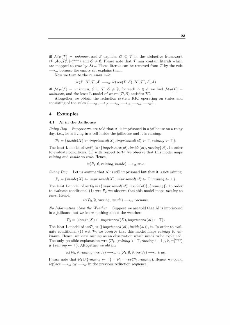
Rainy Day Suppose we are told that Al is imprisoned in a jailhouse on a rainyday, i.e.., he is living in a cell inside the jailhouse and it is raining:

P1 = {inside(X)← imprisoned(X), imprisoned(al)← >, raining ← >}.The least L-model of wcP1 is 〈{imprisoned(al), inside(al), raining}, ∅〉. In orderto evaluate conditional (1) with respect to P1 we observe that this model mapsraining and inside to true. Hence,

ic(P1, ∅, raining , inside) −→it true.

Sunny Day Let us assume that Al is still imprisoned but that it is not raining:

P2 = {inside(X)← imprisoned(X), imprisoned(al)← >, raining ← ⊥}.The least L-model of wcP2 is 〈{imprisoned(al), inside(al)}, {raining}〉. In orderto evaluate conditional (1) wrt P2 we observe that this model maps raining tofalse. Hence,

ic(P2, ∅, raining , inside) −→iv vacuous.

No Information about the Weather Suppose we are told that Al is imprisonedin a jailhouse but we know nothing about the weather:

P3 = {inside(X)← imprisoned(X), imprisoned(al)← >}.The least L-model of wcP1 is 〈{imprisoned(al), inside(al)}, ∅〉. In order to eval-uate conditional (1) wrt P3 we observe that this model maps raining to un-known. Hence, we view raining as an observation which needs to be explained.The only possible explanation wrt 〈P3, {raining ← >, raining ← ⊥}, ∅, |=lmwc

L 〉is {raining ← >}. Altogether we obtain

ic(P3, ∅, raining , inside) −→ia ic(P1, ∅, ∅, inside) −→it true.

Please note that P3 ∪ {raining ← >} = P1 = rev(P3, raining). Hence, we couldreplace −→ia by −→ir in the previous reduction sequence.

23

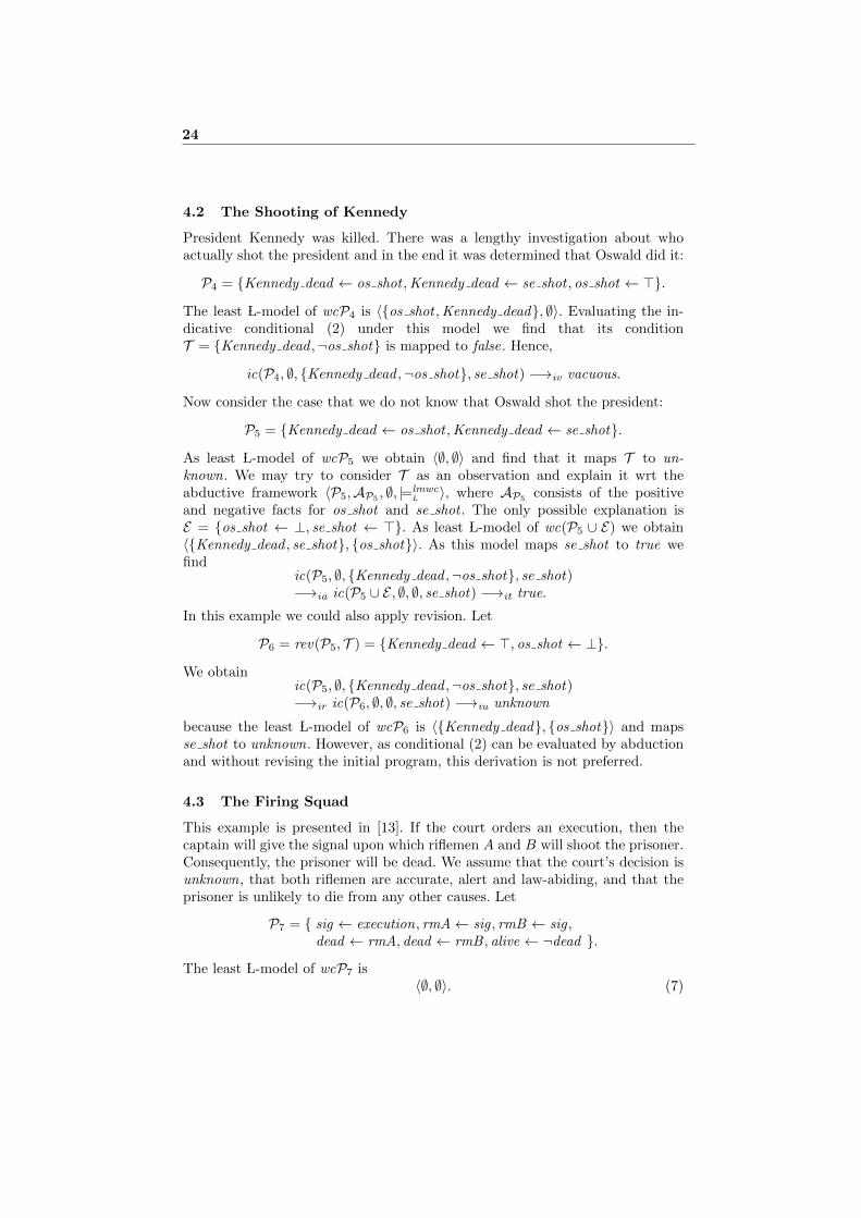
4.2 The Shooting of Kennedy

President Kennedy was killed. There was a lengthy investigation about whoactually shot the president and in the end it was determined that Oswald did it:

P4 = {Kennedy dead ← os shot ,Kennedy dead ← se shot , os shot ← >}.

The least L-model of wcP4 is 〈{os shot ,Kennedy dead}, ∅〉. Evaluating the in-dicative conditional (2) under this model we find that its conditionT = {Kennedy dead ,¬os shot} is mapped to false. Hence,

ic(P4, ∅, {Kennedy dead ,¬os shot}, se shot) −→iv vacuous.

Now consider the case that we do not know that Oswald shot the president:

P5 = {Kennedy dead ← os shot ,Kennedy dead ← se shot}.

As least L-model of wcP5 we obtain 〈∅, ∅〉 and find that it maps T to un-known. We may try to consider T as an observation and explain it wrt theabductive framework 〈P5,AP5 , ∅, |=lmwc

L 〉, where AP5 consists of the positiveand negative facts for os shot and se shot . The only possible explanation isE = {os shot ← ⊥, se shot ← >}. As least L-model of wc(P5 ∪ E) we obtain〈{Kennedy dead , se shot}, {os shot}〉. As this model maps se shot to true wefind

ic(P5, ∅, {Kennedy dead ,¬os shot}, se shot)−→ia ic(P5 ∪ E , ∅, ∅, se shot) −→it true.

In this example we could also apply revision. Let

P6 = rev(P5, T ) = {Kennedy dead ← >, os shot ← ⊥}.

We obtainic(P5, ∅, {Kennedy dead ,¬os shot}, se shot)−→ir ic(P6, ∅, ∅, se shot) −→iu unknown

because the least L-model of wcP6 is 〈{Kennedy dead}, {os shot}〉 and mapsse shot to unknown. However, as conditional (2) can be evaluated by abductionand without revising the initial program, this derivation is not preferred.

4.3 The Firing Squad

This example is presented in [13]. If the court orders an execution, then thecaptain will give the signal upon which riflemen A and B will shoot the prisoner.Consequently, the prisoner will be dead. We assume that the court’s decision isunknown, that both riflemen are accurate, alert and law-abiding, and that theprisoner is unlikely to die from any other causes. Let

P7 = { sig ← execution, rmA← sig , rmB ← sig ,dead ← rmA, dead ← rmB , alive ← ¬dead }.

The least L-model of wcP7 is〈∅, ∅〉. (7)

24

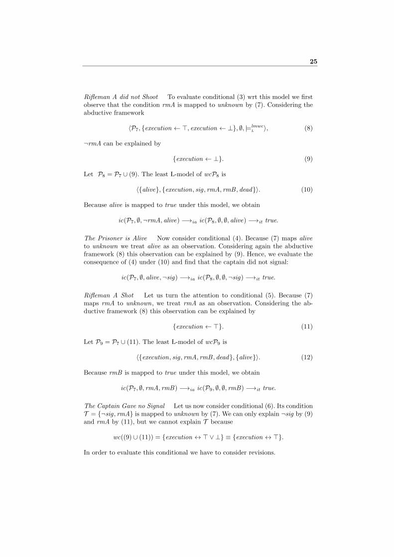
Rifleman A did not Shoot To evaluate conditional (3) wrt this model we firstobserve that the condition rmA is mapped to unknown by (7). Considering theabductive framework

〈P7, {execution ← >, execution ← ⊥}, ∅, |=lmwc L 〉, (8)

¬rmA can be explained by

{execution ← ⊥}. (9)

Let P8 = P7 ∪ (9). The least L-model of wcP8 is

〈{alive}, {execution, sig , rmA, rmB , dead}〉. (10)

Because alive is mapped to true under this model, we obtain

ic(P7, ∅,¬rmA, alive) −→ia ic(P8, ∅, ∅, alive) −→it true.

The Prisoner is Alive Now consider conditional (4). Because (7) maps aliveto unknown we treat alive as an observation. Considering again the abductiveframework (8) this observation can be explained by (9). Hence, we evaluate theconsequence of (4) under (10) and find that the captain did not signal:

ic(P7, ∅, alive,¬sig) −→ia ic(P8, ∅, ∅,¬sig) −→it true.

Rifleman A Shot Let us turn the attention to conditional (5). Because (7)maps rmA to unknown, we treat rmA as an observation. Considering the ab-ductive framework (8) this observation can be explained by

{execution ← >}. (11)

Let P9 = P7 ∪ (11). The least L-model of wcP9 is

〈{execution, sig , rmA, rmB , dead}, {alive}〉. (12)

Because rmB is mapped to true under this model, we obtain

ic(P7, ∅, rmA, rmB) −→ia ic(P9, ∅, ∅, rmB) −→it true.

The Captain Gave no Signal Let us now consider conditional (6). Its conditionT = {¬sig , rmA} is mapped to unknown by (7). We can only explain ¬sig by (9)and rmA by (11), but we cannot explain T because

wc((9) ∪ (11)) = {execution ↔ >∨⊥} ≡ {execution ↔ >}.

In order to evaluate this conditional we have to consider revisions.

25

1. A brute force method is to revise the program wrt all conditions. Let

P10 = rev(P7, {¬sig , rmA})= (P7 \ def ({¬sig , rmA},P7)) ∪ {sig ← ⊥, rmA← >}.

The least L-model of wcP10 is

〈{rmA, dead}, {sig , rmB , alive}〉. (13)

This model maps dead to true and rmB to false and we obtain

ic(P7, ∅, {¬sig , rmA}, {dead ,¬rmB})−→ir ic(P10, ∅, ∅, {dead ,¬rmB}) −→it true.

2. As we prefer minimal revisions let us consider

P11 = rev(P7, rmA) = (P7 \ def (rmA,P7)) ∪ {rmA← >}.The least L-model of wcP11 is 〈{dead , rmA}, {alive}〉. Unfortunately, ¬sigis still mapped to unknown by this model, but it can be explained in the ab-ductive framework 〈P11, {execution ← >, execution ← ⊥}, ∅, |=lmwc

L 〉 by (9).Let P12 = P11 ∪ (9). Because the least L-model of wcP12 is

〈{dead , rmA}, {alive, execution, sig , rmB}〉 (14)

we obtain

ic(P7, ∅, {¬sig , rmA}, {dead ,¬rmB})−→ir ic(P11, ∅,¬sig , {dead ,¬rmB})−→ia ic(P12, ∅, ∅, {dead ,¬rmB} −→it true.

The revision leading to P11 is minimal in the sense that only the definitionof rmA is revised and without this revision the condition of (6) cannot beexplained. This is the only minimal revision as we will show in the sequel.

3. An alternative minimal revision could be the revision of P7 wrt to ¬sig :

P13 = rev(P7,¬sig) = (P7 \ def (¬sig ,P7)) ∪ {sig ← ⊥}.The least L-model of wcP13 is

〈{alive}, {sig , dead , rmA, rmB}〉. (15)

Because this model maps rmA to false we obtain:

ic(P7, ∅, {¬sig , rmA}, {dead ,¬rmB})−→ir ic(P13, ∅, rmA, {dead ,¬rmB}) −→iv vacuous.

4. So far the first step in evaluating the conditional was a revision step. Alter-natively, we could start with an abduction step. ¬sig can be explained inthe abductive framework (8) by (9) leading to the program P8 and the least L-model (10). Because this model maps rmA to false we obtain:

ic(P7, ∅, {¬sig , rmA}, {dead ,¬rmB})−→ia ic(P8, ∅, rmA, {dead ,¬rmB}) −→iv vacuous.

26

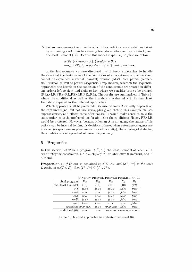
5. Let us now reverse the order in which the conditions are treated and startby explaining rmA. This has already been done before and we obtain P9 andthe least L-model (12). Because this model maps ¬sig to false we obtain:

ic(P7, ∅, {¬sig , rmA}, {dead ,¬rmB})−→ia ic(P9, ∅,¬sig , {dead ,¬rmB}) −→iv vacuous.

In the last example we have discussed five different approaches to handlethe case that the truth value of the conditions of a conditional is unknown andcannot be explained: maximal (parallel) revision (MaxRev), partial (sequen-tial) revision as well as partial (sequential) explanation, where in the sequentialapproaches the literals in the condition of the conditionals are treated in differ-ent orders: left-to-right and right-to-left, where we consider sets to be ordered(PRevLR,PRevRL,PExLR,PExRL). The results are summarized in Table 1,where the conditional as well as the literals are evaluated wrt the final least L-model computed in the different approaches.

Which approach shall be preferred? Because rifleman A causally depends onthe captain’s signal but not vice-versa, plus given that in this example clausesexpress causes, and effects come after causes, it would make sense to take thecause ordering as the preferred one for abducing the conditions. Hence, PExLRwould be preferred. However, because rifleman A is an agent, the causes of hisactions can be internal to him, his decisions. Hence, when autonomous agents areinvolved (or spontaneous phenomena like radioactivity), the ordering of abducingthe conditions is independent of causal dependency.

5 Properties

In this section, let P be a program, 〈I>, I⊥〉 the least L-model of wcP, IC aset of integrity constraints, 〈P,AP , IC, |=lmwc

L 〉 an abductive framework, and La literal.

Proposition 1. If O can be explained by E ⊆ AP and 〈J>, J⊥〉 is the least L-model of wc(P ∪ E), then 〈I>, I⊥〉 ⊆ 〈J>, J⊥〉.

MaxRev PRevRL PRevLR PExLR PExRL

final program P10 P12 P13 P8 P9

final least L-model (13) (14) (15) (10) (12)

sig false false false false truermA true true false false true

dead true true false false truermB false false false false true

alive false false true true falseexecution unknown false unknown false true

conditional (6) true true vacuous vacuous vacuous

Table 1. Different approaches to evaluate conditional (6).

27

Proof. The least L-models 〈I>, I⊥〉 and 〈J>, J⊥〉 are the least fixed points ofthe semantic operators ΦP and ΦP∪E , respectively. Let 〈I>n , I⊥n 〉 and 〈J>n , J⊥n 〉be the interpretations obtained after applying ΦP and ΦP∪E n-times to 〈∅, ∅〉,respectively. We can show by induction on n that 〈I>n , I⊥n 〉 ⊆ 〈J>n , J⊥n 〉. Theproposition follows immediately.

Proposition 1 guarantees that whenever −→ia is applied, previously checkedconditions of a conditional need not to be re-checked. The following Proposition 3gives the same guarantee whenever −→ir is applied.

Proposition 2. If the least L-model of wcP maps L to unknown and 〈J>, J⊥〉is the least L-model of wc rev(P, L), then 〈I>, I⊥〉 ⊂ 〈J>, J⊥〉.Proof. By induction on the number of applications of ΦP and Φrev(P,L).

Proposition 3. RIC is terminating.

Proof. Each application of −→it , −→if , −→iu or −→iv leads to an irreducibleexpression. Let cond(T ,A) be the conditional to which RIC is applied. When-ever −→ir is applied then the definition of at least one literal L occurring in T isrevised such that the least L-model of the weak completion of revised programmaps L to true. Because T does not contain a complementary pair of literalsthis revised definition of L is never revised again. Hence, there cannot exist arewriting sequence with infinitely many occurrences of −→ir . Likewise, therecannot exist a rewriting sequence with infinitely many occurrences of −→ia be-cause each application of −→ia to a state ic(P, IC, T ,A) reduces the number ofliterals occurring in the T .

Proposition 4. RIC is not confluent.

Proof. This follows immediately from the examples presented in Section 4.

6 Open Questions and the Proposal of an Experiment

Open Questions The new approach gives rise to a number of questions. Whichof the approaches is preferable? This may be a question of pragmatics imputableto the user. The default, because no pragmatic information has been added, ismaximals revision for skepticism and minimal revisions for credulity. Do humansevaluate multiple conditions sequentially or in parallel? If multiple conditionsare evaluated sequentially, are they evaluated by some preferred order? Shallexplanations be computed skeptically or credulously? How can the approach beextended to handle subjunctive conditionals?

The Proposal of an Experiment Subjects are given the background informa-tion specified in the program P9. They are confronted with the conditionalslike (6) as well as variants with different consequences (e.g., execution insteadof {dead ,¬rmB} or conditionals where the order of two conditions are reversed.We then ask the subjects to answer questions like: Does the conditional hold?or Did the court order an execution? Depending on the answers we may learnwhich approaches are preferred by humans.

28

Acknowledgements We thank Bob Kowalski for valuable comments on an ear-lier draft of the paper.

References

1. E.-A. Dietz, S. Holldobler, and M. Ragni. A computational logic approach tothe abstract and the social case of the selection task. In Proceedings EleventhInternational Symposium on Logical Formalizations of Commonsense Reasoning,2013.

2. E.-A. Dietz, S. Holldobler, and M. Ragni. A computational logic approach to thesuppression task. In N. Miyake, D. Peebles, and R. P. Cooper, editors, Proceedingsof the 34th Annual Conference of the Cognitive Science Society, pages 1500–1505.Cognitive Science Society, 2012.

3. E.-A. Dietz, S. Holldobler, and C. Wernhard. Modelling the suppression task underweak completion and well-founded semantics. Journal of Applied Non-ClassicalLogics, 24:61–85, 2014.

4. M. L. Ginsberg. Counterfactuals. Artificial Intelligence, 30(1):35–79, 1986.5. S. Holldobler and C. D. P. Kencana Ramli. Contraction properties of a semantic

operator for human reasoning. In Lei Li and K. K. Yen, editors, Proceedings ofthe Fifth International Conference on Information, pages 228–231. InternationalInformation Institute, 2009.

6. S. Holldobler and C. D. P. Kencana Ramli. Logic programs under three-valued Lukasiewicz’s semantics. In P. M. Hill and D. S. Warren, editors, Logic Pro-gramming, volume 5649 of Lecture Notes in Computer Science, pages 464–478.Springer-Verlag Berlin Heidelberg, 2009.

7. S. Holldobler and C. D. P. Kencana Ramli. Logics and networks for human rea-soning. In C. Alippi, Marios M. Polycarpou, Christos G. Panayiotou, and GeorgiosEllinasetal, editors, Artificial Neural Networks – ICANN, volume 5769 of LectureNotes in Computer Science, pages 85–94. Springer-Verlag Berlin Heidelberg, 2009.

8. S. Holldobler, T. Philipp, and C. Wernhard. An abductive model for hu-man reasoning. In Proceedings Tenth International Symposium on Logi-cal Formalizations of Commonsense Reasoning, 2011. commonsensereason-ing.org/2011/proceedings.html.

9. A. C. Kakas, R. A. Kowalski, and F. Toni. Abductive Logic Programming. Journalof Logic and Computation, 2(6):719–770, 1993.

10. D. Lewis. Counterfactuals. Blackwell Publishers, Oxford, 1973.11. J. W. Lloyd. Foundations of Logic Programming. Springer, Berlin, Heidelberg,

1987.12. J. Lukasiewicz. O logice trojwartosciowej. Ruch Filozoficzny, 5:169–171, 1920.

English translation: On Three-Valued Logic. In: Jan Lukasiewicz Selected Works.(L. Borkowski, ed.), North Holland, 87-88, 1990.

13. J. Pearl. Causality: Models, Reasoning, and Inference. Cambridge University Press,New York, USA, 2000.

14. L. M. Pereira and J. N. Aparıcio. Relevant counterfactuals. In Proceedings 4thPortuguese Conference on Artificial Intelligence (EPIA), volume 390 of LectureNotes in Computer Science, pages 107–118. Springer, 1989.

15. L. M. Pereira, E.-A. Dietz, and S. Holldobler. An abductive reasoning approach tothe belief-bias effect. In C. Baral, G. De Giacomo, and T. Eiter, editors, Principlesof Knowledge Representation and Reasoning: Proceedings of the 14th InternationalConference, pages 653–656, Cambridge, MA, 2014. AAAI Press.

29

16. L. M. Pereira, E.-A. Dietz, and S. Holldobler. Contextual abductive reasoningwith side-effects. In I. Niemela, editor, Theory and Practice of Logic Programming(TPLP), volume 14, pages 633–648, Cambridge, UK, 2014. Cambridge UniversityPress.

17. F. Ramsey. The Foundations of Mathematics and Other Logical Essays. Harcourt,Brace and Company, 1931.

18. N. Rescher. Conditionals. MIT Press, Cambridge, MA, 2007.19. K. Stenning and M. van Lambalgen. Human Reasoning and Cognitive Science.

MIT Press, 2008.

30

The Logical Difference for EL:from Terminologies towards TBoxes?

Shasha Feng1, Michel Ludwig2, and Dirk Walther2

1 Jilin University, Chinafengss@jlu.edu.cn

2 Theoretical Computer ScienceTU Dresden, Germany

{michel,dirk}@tcs.inf.tu-dresden.de

Abstract. In this paper we are concerned with the logical differenceproblem between ontologies. The logical difference is the set of subsump-tion queries that follow from a first ontology but not from a second one.We revisit our solution to logical difference problem for EL-terminologiesbased on finding simulations between hypergraph representations of theterminologies, and we investigate a possible extension of the method togeneral EL-TBoxes.

1 Introduction

Ontologies are widely used to represent domain knowledge. They contain spec-ifications of objects, concepts and relationships that are often formalised usinga logic-based language over a vocabulary that is particular to an applicationdomain. Ontology languages based on description logics [2] have been widelyadopted, e.g., description logics are underlying the Web Ontology Language(OWL) and its profiles.3 Numerous ontologies have already been developed, inparticular, in knowledge intensive areas such as the biomedical domain, and theyare made available in dedicated repositories such as the NCBO bioportal.4

Ontologies constantly evolve, they are regularly extended, corrected and re-fined. As the size of ontologies increases, their continued development and main-tenance becomes more challenging as well. In particular, the need to have auto-mated tool support for detecting and representing differences between versionsof an ontology is growing in importance for ontology engineering.

The logical difference is taken to be the set of queries that produce differ-ent answers when evaluated over distinct versions of an ontology. The languageand vocabulary of the queries can be adapted in such a way that exactly thedifferences of interest become visible, which can be independent of the syntac-tic representation of the ontologies. We consider ontologies formulated in the

? The second and third authors were supported by the German Research Foundation(DFG) within the Cluster of Excellence ‘Center for Advancing Electronics Dresden’.

3 http://www.w3.org/TR/owl2-overview/4 http://bioportal.bioontology.org

lightweight description logic EL [1, 3] and queries that are EL-concept inclu-sions. The relevance of EL for ontologies is emphasised by the fact that manyontologies are largely formulated in EL. For instance, the dataset of the ORE2014 reasoner evaluation comprises 8 805 OWL-EL ontologies.5

The logical difference problem was introduced in [7] and investigated forEL-terminologies [6]. A hypergraph-based approach for EL-terminologies waspresented in [4], which was subsequently extended to EL-terminologies with ad-ditional role inclusions, domain and range restrictions of roles in [8]. In thispaper we investigate a possible extension of the method to general EL-TBoxes.Clearly, such an extension needs to account for the additional expressivity ofgeneral TBoxes w.r.t. terminologies. After normalisation, a terminology maycontain at most one axiom of the form ∃r.A v X or A1 u . . . u An v X for anyconcept name X, whereas a general TBox does not impose such a restriction.

We first show that for every concept inclusion C v D that follows from aTBox T , there exists a concept name X in T that acts as an interpolant betweenthe concepts C and D, i.e., we have that T |= C v X and T |= X v D. Then wedescribe the set of all subsumees C of X in T using a concept of EL extendedwith disjunction and a least fixpoint operator, and the set of all subsumers D ofX in T using a concept of EL extended with greatest fixpoint operators. Finally,we reduce the problem of deciding the logical difference between two EL-TBoxesto fixpoint reasoning w.r.t. TBoxes in a hybrid µ-calculus [10].

The paper is organised as follows. We start by recalling some notions re-garding the description logic EL and its extensions with disjunction and fix-point operators. In Section 3, we discuss how the logical difference problem forEL-terminologies could be extended to general EL-TBoxes, and we establish awitness theorem for general EL-TBoxes. In Section 4, we show how fixpointreasoning can be used to decide whether two general EL-TBoxes are logicallydifferent, and how witnesses to the logical difference can be computed. Finallywe conclude the paper.

2 Preliminaries

We start by briefly reviewing the lightweight description logic EL and somenotions related to the logical difference, together with some basic results.

Let NC, NR, and NV be mutually disjoint sets of concept names, role names,and variable names, respectively. We assume these sets to be countably infinite.We typically use A,B to denote concept names and r to denote role names.

The sets of EL-concepts C, ELUµ-concepts D, and ELν-concepts E are builtaccording to the following grammar rules:

C ::= > | A | C u C | ∃r.CD ::= > | A | D uD | D tD | ∃r.D | x | µx.DE ::= > | A | E u E | ∃r.E | x | νx.E

5 http://dl.kr.org/ore2014/

32

where A ∈ NC, r, s ∈ NR, and x ∈ NV. For an ELUµ-concept C, the set of freevariables in C, denoted by FV(C) is defined inductively as follows: FV(>) = ∅,FV(A) = ∅, FV(D1 u D2) = FV(D1) ∪ FV(D2), FV(D1 t D2) = FV(D1) ∪FV(D2), FV(∃r.D′) = FV(D′), FV(x) = {x}, FV(µx.D′) = FV(D′) \ {x}.The set FV(E) of free variables occurring in an ELν-concept E can be definedanalogously. An ELUµ-concept C (an ELν-concept D) is closed if C (D) doesnot contain free occurrences of variables, i.e. FV(C) = ∅ (FV(D) = ∅). In thefollowing we assume that every ELUµ-concept C and every ELν-concept D isclosed.

An EL-TBox T is a finite set of axioms, where an axiom can be a conceptinclusion C v C ′, or a concept equation C ≡ C ′, where C,C ′ range over EL-concepts. An EL-terminology T is an EL-TBox consisting of axioms α of theform A v C and A ≡ C, where A is a concept name, C an EL-concept and noconcept name A occurs more than once on the left-hand side of an axiom.

The semantics of EL, ELUµ, and ELν is defined using interpretations I =(∆I , ·I), where the domain ∆I is a non-empty set, and ·I is a function mappingeach concept name A to a subset AI of ∆I and every role name r to a binaryrelation rI ⊆ ∆I×∆I . Interpretations are extended to concepts using a function·I,ξ that is parameterised by an assignment function that maps variables x ∈ NV

to sets ξ(x) ⊆ ∆I . Given an assignment ξ, the extension of an EL, ELUµ, orELν-concept is defined inductively as follows: >I,ξ := ∆I , xI,ξ := ξ(x) forx ∈ NV, (C1 u C2)I,ξ := CI

1 ∩ CI2 , (∃r.C)I,ξ := {x ∈ ∆I | ∃y ∈ CI,ξ : (x, y) ∈

rI }, (µx.C)I,ξ =⋂{W ⊆ ∆I | CI,ξ[x 7→W ] ⊆ W }, and (νx.C)I,ξ =

⋃{W ⊆∆I | W ⊆ CI,ξ[x 7→W ] }, where ξ[x 7→ W ] denotes the assignment ξ modified bymapping x to W .

An interpretation I satisfies a concept C, an axiom C v D or C ≡ D if,respectively, CI,∅ 6= ∅, CI,∅ ⊆ DI , or CI,∅ = DI,∅. We write I |= α iff Isatisfies the axiom α. An interpretation I satisfies a TBox T iff I satisfies allaxioms in T ; in this case, we say that I is a model of T . An axiom α followsfrom a TBox T , written T |= α, iff for all models I of T , we have that I |= α.Deciding whether T |= C v C ′, for two EL-concepts C and C ′, can be done inpolynomial time in the size of T and C,C ′ [1, 3]. For an ELUµ-concept D andan ELν-concept E, it is known that T |= D v E can be decided in exponentialtime in the size of T , D and E [10].

A signature Σ is a finite set of symbols from NC and NR. The signaturesig(C), sig(α) or sig(T ) of the concept C, axiom α or TBox T is the set ofconcept and role names occurring in C, α or T , respectively. An ELΣ-concept Cis an EL-concept such that sig(C) ⊆ Σ.

An EL-TBox T is normalised if it only contains EL-concept inclusions of theforms > v B, A1 u . . . uAn v B, A v ∃r.B, or ∃r.A v B, where A,Ai, B ∈ NC,r ∈ NR, and n ≥ 1. Every EL-TBox T can be normalised in polynomial time inthe size of T with a linear increase in the size of the normalised TBox w.r.t. Tsuch that the resulting TBox is a conservative extension of T [6]. Note that ina normalised terminology T , we have that for every axiom of the form ∃r.A vB ∈ T , there exists an axiom of the form B v ∃r.A ∈ T ; similarly for axioms of

33

the form A1 u . . . u An v B with n ≥ 2. When convenient, we will abbreviatetwo axioms A v ∃r.B and ∃r.B v A by the single axiom A ≡ ∃r.B; similarly forA ≡ B1 u . . . uBn.

3 Towards Logical Difference between GeneralEL-TBoxes

The logical difference between two TBoxes witnessed by concept inclusions overa signature Σ is defined as follows.

Definition 1. The Σ-concept difference between two EL-TBoxes T1 and T2 fora signature Σ is the set cDiffΣ(T1, T2) of all EL-concept inclusions α such thatsig(α) ⊆ Σ, T1 |= α, and T2 6|= α.

EL-TBoxes can be translated into directed hypergraphs by taking the sig-nature symbols as nodes and treating the axioms as hyperedges connectingthe nodes. For normalised EL-TBoxes, the axiom > v B is translated intothe hyperedge ({x>}, {xB}), the axiom A1 u . . . u An v B into the hyperedge({xB1 , . . . , xBn}, {xA}), the axiomA v ∃r.B into the hyperedge ({xA}, {xr, xB}),and the axiom ∃r.A v B into the hyperedge ({xr, xB}, {xA}), where each nodexY corresponds to the signature symbol Y , respectively. A feature of the trans-lation of axioms into hyperedges is that all information about the axiom andthe logical operators in it is preserved. In fact we can treat the ontology and itshypergraph representation interchangeably. The existence of certain simulationsbetween hypergraphs for EL-terminologies characterises the fact that the corre-sponding terminologies are logically equivalent and, thus, no logical differenceexists [4, 8].

As the set cDiffΣ(T1, T2) is infinite in general, we make use of the following“primitive witnesses” theorem from [6] that states that we only have to con-sider two specific types of concept differences. If there is an inclusion C v D ∈cDiffΣ(T1, T2) for two terminologies T1 and T2, then we know that there is a con-cept name A ∈ Σ such that A occurs either on the left-hand or the right-handside of an inclusion in the set C v D ∈ cDiffΣ(T1, T2). For checking whethercDiffΣ(T1, T2) = ∅, we only have to consider such simple inclusions. However, ifT1 and T2 are general EL-TBoxes, the situation is different.

Example 1. Let T1 = {X ≡ A1 u A2, X v ∃r.>}, T2 = ∅, and let Σ ={A1, A2, r}. Note that T1 is not a terminology as the concept name X occurstwice on the left-hand side of an axiom. Then every difference α ∈ cDiffΣ(T1, T2)is equivalent to the inclusion A1 uA2 v ∃r.>. In particular, there does not exista difference of the form ψ v θ, where ψ or θ is a concept name from Σ.

As illustrated by the example, we need to account for a new kind of differencesC v C ′ ∈ cDiffΣ(T1, T2) which are induced by a concept name X ∈ sig(T1)such that X 6∈ Σ, T1 |= C v X, and T1 |= X v C ′. We obtain the followingwitness theorem for EL-TBoxes as an extension of the witness theorem for EL-terminologies.

34

Theorem 1 (Witness Theorem). Let T1, T2 be two normalised EL-TBoxesand let Σ be a signature. Then, cDiffΣ(T1, T2) 6= ∅ iff there exists an ELΣ-inclusion α = ϕ v ψ such that T1 |= α and T2 6|= α, where

(i) ϕ is an ELΣ-concept and ψ = A ∈ Σ,(ii) ϕ = A ∈ Σ and ψ is an ELΣ-concept, or

(iii) there exists X ∈ sig(T1) \Σ such that T1 |= ϕ v X and T1 |= X v ψ.

The proof of the witness theorem for terminologies [6] is based on analysingthe subsumption T1 |= ϕ v ψ syntactically, using a sequent calculus [5]. A similartechnique can be used for the proof of Theorem 2.

For deciding whether cDiffΣ(T1, T2) = ∅ in the case of general TBoxes, we nowhave to additionally consider differences of Type (iii). Differences of types (i)or (ii) can be checked by using forward or backward simulations adapted tonormalised EL-TBoxes, respectively, whereas Type (iii) differences require acombination of both techniques.

Before we illustrate how Type (iii) differences can be dealt with, we firstintroduce some auxiliary notions. We define cWtnlhs

Σ (T1, T2) as the set of allconcept names A from Σ such that there exists an ELΣ-concept C with A vC ∈ cDiffΣ(T1, T2). Similarly, cWtnrhs

Σ (T1, T2) is the set of all concept namesA ∈ Σ such that there exists an ELΣ-concept C with C v A ∈ cDiffΣ(T1, T2).The concept names in cWtnlhs

Σ (T1, T2) are called left-hand side witnesses andthe concept names in cWtnrhs

Σ (T1, T2) right-hand side witnesses. Additionally, wedefine cWtnmid

Σ (T1, T2) as the set of all concept names X from sig(T1) but notfrom Σ such that there exists C v C ′ ∈ cDiffΣ(T1, T2) and T1 |= C v X andT1 |= X v C ′. The concept names in cWtnmid

Σ (T1, T2) are called interpolatingwitnesses. To summarise, we have the following sets:

cWtnlhsΣ (T1, T2) = {A ∈ Σ | ∃C ∈ ELΣ : A v C ∈ cDiffΣ(T1, T2) }

cWtnrhsΣ (T1, T2) = {A ∈ Σ | ∃C ∈ ELΣ : C v A ∈ cDiffΣ(T1, T2) }

cWtnmidΣ (T1, T2) = {X ∈ sig(T1) \Σ | ∃C,C ′ ∈ ELΣ : T1 |= C v X,

T1 |= X v C ′, T2 6|= C v C ′ }

We illustrate the witness sets with the following example.

Example 2. Let T1 = {X ≡ A1 u A2, X v ∃r.>, A3 v A2, A3 v ∃r.A2}, T2 ={A2 v ∃r.>}, and let Σ = {A1, A2, r}. Then it holds that cWtnlhs

Σ (T1, T2) = {A3}(e.g. {A3 v A2, A3 v ∃r.A2} ⊆ cDiffΣ(T1, T2)), cWtnrhs

Σ (T1, T2) = {A2} (e.g.A3 v A2 ∈ cDiffΣ(T1, T2)), and cWtnmid

Σ (T1, T2) = {X} (e.g. T1 |= A1 uA3 v X,T1 |= X v ∃r.> and T2 6|= A1 uA3 v ∃r.>).

We obtain as a corollary of Theorem 2 that, to decide the logical differencebetween two EL-TBoxes, it is sufficient to check the emptiness of the witnesssets.

Corollary 1. Let T1, T2 be two normalised EL-TBoxes and let Σ be a signature.Then it holds that cDiffΣ(T1, T2) = ∅ iff cWtnlhs

Σ (T1, T2) = cWtnrhsΣ (T1, T2) =

cWtnmidΣ (T1, T2) = ∅.

35

To characterise an interpolating witness of a Type-(iii) difference, we usethe sets of its of subsumees and subsumers formulated using certain signaturesymbols only. A similar approach was used for the construction of uniform in-terpolants of EL-TBoxes in [9].

Definition 2. Let T be an EL-TBox, let Σ be a signature and let C be anEL-concept. We define PremisesΣT (C) := {E ∈ ELΣ | T |= E v C } andConclusionsΣT (C) := {E ∈ ELΣ | T |= C v E }.The set PremisesΣT (C) contains all EL-concepts formulated using Σ-symbols onlythat entail C w.r.t. T ; or are entailed by C in the case of ConclusionsΣT (C). Theelements of PremisesΣT (C) are also called Σ-implicants or Σ-subsumees of Cw.r.t. T , and the elements of ConclusionsΣT (C) are also named Σ-implicates orΣ-subsumers of C w.r.t. T .

In [4], it was established that a concept name X is forward simulated by aconcept name Y in an EL-terminology T iff it holds that ConclusionsΣT (X) ⊆ConclusionsΣT (Y ); and similary,X is backward simulated by Y iff PremisesΣT (X) ⊆PremisesΣT (Y ). We aim now at lifting this result to general EL-TBoxes.

Example 3. Let T1 = {A v X, ∃r.X v X, X v B1, X v B2} and T2 = {A vY, ∃r.Y v Y ′, ∃r.Y ′ v Y, ∃r.Y v Z1, ∃r.Y v Z2, Y v B1, Y v B2, Z1 vB1, Z2 v B2} be two EL-TBoxes. Let Σ = {A,B1, B2, r} be a signature. Notethat X in T1 is cyclic and intuitively, the interpretation of X in a model I of T1contains all finite r-chains “ending in A”. In T2 the concept name Y is cyclicand its interpretation contains all r-chains ending in A that are of even length,whereas the interpretations of the concept names Z1 and Z2 contain all r-chainsending in A that are of odd length. Formally, we have that:

{A,∃r.A, ∃r.∃r.A, . . . } ⊆ PremisesΣT1(X)

{A, ∃r.∃r.A, ∃r.∃r.∃r.∃r.A, . . . } ⊆ PremisesΣT2(Y )

{∃r.A, ∃r.∃r.∃r.A, . . . } ⊆ PremisesΣT2(Zi) for i ∈ {1, 2}

In particular, for i ∈ {1, 2}, we have

PremisesΣT1(X) = PremisesΣT2

(Y ) ∪ PremisesΣT2(Zi).

Intuitively, the set of Σ-implicants of X in T1 are distributed over the conceptnames Y and Zi in T2. Moreover it holds that

ConclusionsΣT1(X) = ConclusionsΣT2

(Y ) = ConclusionsΣT2(Z1 u Z2).

The concept name X in T1 could be forward simulated either by Y or Z1 u Z2

in T2. Note that Z1 or Z2 individually are not sufficient. Analogously, X could bebackward simulated by Y tZ1 or Y tZ2. None of the concept names X, Z1, orZ2 are sufficient individually for the backward simulation. Combining backwardand forward simulation, X could be simulated by Y t (Z1 u Z2).

In general, we hypothesise that non-Σ-concept names X in T1 need to be“simulated” by concepts of the form

⊔ni=1 Ci, where Ci are EL-concepts.

36

4 Finding Logical Differences via Fixpoint Reasoning

We now show how fixpoint reasoning can be used to find difference witnessesbetween general EL-TBoxes.

Given Theorem 2, we know that any difference C v C ′ ∈ cDiffΣ(T1, T2), fortwo ELΣ-concepts C and C ′, is connected to some concept name X occurringin T1 for which either T1 |= C v X, or T1 |= X v C ′ (or both) holds. To checkwhether X is indeed a difference witness, we construct concepts BΣT1

(X) and

FΣT1(X) formulated in ELUΣµ and in ELΣν , respectively, to describe the (poten-

tially infinite) disjunction of Σ-concepts that are subsumed by X w.r.t. T1, andthe conjunction of all the Σ-concepts that subsume X w.r.t. T1, respectively.Note that the use of fixpoint allows for a finite description of infinite disjunc-tions or conjunctions. The ELUΣµ -concept BΣT1

(X) hence is a finite representation

of the set PremisesΣT1(X), whereas the ELΣν -concept FΣT1

(X) represents the set

PremisesΣT1(X) in a finite way. Using the fixpoint descriptions of the premises

and conclusions of X w.r.t. T1, we can verify whether X is a difference witnessby checking T2 |= BΣT1

(X) v FΣT1(X).

We first turn our attention to the set PremisesΣT1(X). Before we can give a

formal definition for the concept BΣT1(X), we have to introduce the following

auxiliary notion to handle concept names X in the definition of BΣT1(X) for

which there exist axioms of the form Z1 u . . .uZn v Z in a normalised TBox Tsuch that T |= Z v X. Intuitively, given a concept name X, we construct aset ConjT (X) containing sets of concept names which has the property that forevery EL-concept D with T |= D v X, there exists a set S = {Y1, . . . , Ym} ∈ConjT (X) such that T |= D v Yi follows without involving any axioms of theform Z1 u . . . u Zn v Z. Nested implications between such axioms also have tobe taken into account.

Definition 3. Let T be a normalised EL-TBox and let X ∈ NC. We define theset ConjT (X) ⊆ 2sig(T )∩NC to be smallest set inductively defined as follows:

– {X} ∈ ConjT (X);– if S ∈ ConjT (X), Y ∈ S, and Z1 u . . . u Zn v Z ∈ T such that n ≥ 2 andT |= Z v Y , then S \ {Y } ∪ {Z1, . . . , Zn} ∈ ConjT (X).

Note that for every concept name X the set ConjT (X) is finite as sig(T )∩NC

is finite.

Example 4. Let T1 = {A v X,∃r.X v X}. Then ConjT1(X) = {{X}}. For

T2 = {X1 uX2 v X, X3 uX4 v X1, Y1 u Y2 v X}, we have that

ConjT2(X) = {{X}, {X1, X2}, {X3, X4, X2}, {Y1, Y2}}.

We can now give a formal definition of the concept BΣT (X).

Definition 4. Let T be a normalised EL-TBox, let Σ be a signature, and letX ∈ sig(T ). For a mapping η : NC → NV, we define a closed ELUµΣ-concept

BΣT (X, η) as follows. We set BΣT (X, η) = > if T |= > v X; otherwise BΣT (X, η)is defined recursively in the following way:

37

– If X ∈ dom(η), thenBΣT (X, η) = η(X)

– If X 6∈ dom(η), we set

BΣT (X, η) = µx.⊔

S∈ConjT (X)S={Y1,...,Ym}

(Y ′1 u . . . u Y ′

m)

where x is a fresh variable, and Y ′i (1 ≤ i ≤ n) is defined as follows for

η′ := η ∪ {X 7→ x}:

Y ′i =

⊔

T |=BvYi

B∈Σ

B t⊔

∃r.ZvY ∈Tr∈Σ

T |=YvYi

∃r.BΣT (Z, η′)

Finally, we set BΣT (X) = BΣT (X, ∅).Intuitively, the construction of BΣT (X) starts from X and recursively collects

all the concept names contained in Σ and all the left-hand sides of axioms in Tthat could be relevant for X to be entailed by a concept w.r.t. T . By takinginto account all possible axioms that could lead to a logical entailment, it isguaranteed that we capture every Σ-concept from which X follows w.r.t. T .Reasoning involving axioms of the form Z1 u . . .uZn v Z is handled by the setConjT (X). Infinite recursion over concepts of the form ∃r.C is avoided by keepingtrack of the concept names that been visited already using the mapping η.

We note that for a normalised EL-terminology T , the concept BΣT (X) is of asimpler form than for normalised EL-TBoxes. This is because the concept nameX can occur on the right-hand side of at most one axiom of the form ∃r.A v Xor A1 u . . . u An v X with n ≥ 2 in T , whereas in a TBox several such axiomsmay occur.

We illustrate the concept BΣT (X) with the following examples.

Example 5. Let T1 = {A1 u A2 v X, A3 v A2,∃r.A2 v A1,∃r.A2 v X}, T2 =T1 ∪ {∃r.X v A2}, and let Σ = {A1, A2, A3, r}. We obtain the following ELUµΣ-concepts. We write ϕ instead of µx.ϕ if x does not occur freely in ϕ.

BΣT1(A1) = A1 t ∃r.(A2 tA3) BΣT1

(A2) = A2 tA3

BΣT1(X) = ((A1 t ∃r.(A2 tA3)) u (A2 tA3)) t ∃r.(A2 tA3)

BΣT2(X) = µx.(((A1 t ∃r.(A2 tA3 t ∃r.x)) u (A2 tA3 t ∃r.x))

t ∃r.(A2 tA3 t ∃r.x))

Example 6. Let T1, T2 be defined as in Example 3, and let Σ = {A,B1, B2, r}.We have that for i ∈ {1, 2}:

BΣT1(X) = µx.(A t ∃r.x) BΣT1

(Bi) = Bi tA t ∃r.µx.(A t ∃r.x)

BΣT2(Y ) = µy.(A t ∃r.∃r.y) BΣT2

(Zi) = ∃r.µy.(A t ∃r.∃r.y)

BΣT2(Bi) = Bi tA t ∃r.µy1.(∃r.(A t ∃r.y1)) t ∃r.µy2.(A t ∃r.∃r.y2)

38

By inspecting Definition 4 it is easy to see that |= BΣT (X) ≡ ⊥ if there doesnot an ELΣ-concept C with T |= C v X. Overall, one can establish the followingcorrectness and completeness properties.

Lemma 1. Let T be a normalised EL-TBox, let Σ be a signature, and let X ∈sig(T ). Then the ELUΣµ -concept BΣT (X) satisfies the following properties:

(i) T |= BΣT (X) v X, and(ii) for every D ∈ PremisesΣT (X),

T |= D v X iff |= D v BΣT (X).

The following lemma states that the ELUµ-concept BΣT (X) exactly captures

the infinite set PremisesΣT (X). More formally, the concept BΣT (X) is equivalent tothe infinite disjunction over all the concepts contained in the set PremisesΣT (X).

Lemma 2. Let T be a normalised EL-TBox, let Σ be a signature, and let X ∈sig(T ). Then for every interpretation I it holds that

(BΣT (X))I,∅ =⋃{CI,∅ | C ∈ PremisesΣT (X) }.

Analogously to the concept BΣT (X), it is possible to construct an ELΣν -concept FΣT (X) which exactly captures the set ConclusionsΣT (X) for a conceptname X and an EL-TBox T . Due to lack of space, we cannot give a full definitionof the concept FΣT (X). Instead, we state its existence and its essential propertyin the following lemma.

Lemma 3. Let T be a normalised EL-TBox, let Σ be a signature, and letX ∈ sig(T ). Then there exists an ELν-concept FΣT (X) such that for every inter-pretation I it holds that

(FΣT (X))I,∅ =⋃{CI,∅ | C ∈ ConclusionsΣT (X) }.

We can now state the following theorem, which establishes how the conceptsBΣT (X) and FΣT (X) can be used to search for difference witnesses.

Theorem 2. Let T1, T2 be two normalised EL-TBoxes. Then it holds that:

(i) A 6∈ cWtnlhsΣ (T1, T2) iff T2 |= A v FΣT1

(A), for every A ∈ Σ;

(ii) A 6∈ cWtnrhsΣ (T1, T2) iff T2 |= BΣT1

(A) v A, for every A ∈ Σ; and

(iii) X 6∈ cWtnmidΣ (T1, T2) iff T2 |= BΣT1

(X) v FΣT1(X), for every X ∈ sig(T1)\Σ.

Theorem 2 together with Corollary 1 give rise to an algorithm for deciding thelogical difference between EL-TBoxes. Procedure 1 is such an algorithm basedon reasoning in the hybrid µ-calculus, which allows for fixpoint reasoning w.r.t.TBoxes [10].

Theorem 3. Procedure 1 runs in ExpTime.

39

Procedure 1 Deciding existence of logical difference

Input: Normalised EL-TBoxes T1, T2 and signature Σ

Output: true or false

1: for every concept name X ∈ sig(T1) ∪Σ do

2: B := BΣT1(X)

3: F := FΣT1(X)

4: if X ∈ Σ then

5: if T2 6|= X v F or T2 6|= B v X then

6: return true

7: end if

8: else if T2 6|= B v F then

9: return true

10: end if

11: end for

12: return false

We note that the lower bound for the running time of Procedure 1 may also beexponential as the underlying problem of deciding the logical difference of twoEL-TBoxes is ExpTime-complete [6, 7].

Example 7. Continue Example 3, where sig(T1) ∪ Σ = {A,X,B1, B2, r}. ForA, B = BΣT1

(A) = A, and F = FΣT1(A) = B1 u B2. As T2 |= A v F and

T2 |= B v A, the loop continues. Then for X, B = BΣT1(X) = µx.(A t ∃r.x)

and F = FΣT1(X) = B1 u B2 (cf. Example 6). Since it holds that T2 |= B v F ,

the loop continues. For B1, B = B1 t A t ∃r.µx.(A t ∃r.x) and F = B1. AsT2 |= B1 v F and T2 |= B v B1, the loop continues. The case of B2 is similar tothat of B1. Finally, the algorithm returns false.

Procedure 1 can be modified to obtain witnesses to difference subsumption.

Example 8. We run Procedure 1 on T1, T3 = T2\{Z1 v B1} and Σ, where T1, T2and Σ are the same as in Example 3. Then, for X, we have that B = BΣT1

(X) =

µx.(A t ∃r.x) and F = FΣT1(X) = B1 uB2. However, T3 6|= B v F , which means

X ∈ cWtnmidΣ (T1, T3). Similarly, it can readily be seen that B1 ∈ cWtnrhs

Σ (T1, T3).

5 Conclusion

We have revisited our solution to logical difference problem for EL-terminologieswhich was based on finding simulations between hypergraph representations ofthe terminologies [4]. We have shown that there is a new type of witness inthe logical difference between two EL-TBoxes. We have shown that deciding thelogical difference between two EL-TBoxes can be reduced to fixpoint reasoningw.r.t. TBoxes.

40

References

1. Baader, F., Brandt, S., Lutz, C.: Pushing the EL envelope. In: Proceedings ofthe Nineteenth International Joint Conference on Artificial Intelligence IJCAI-05.Morgan-Kaufmann Publishers, Edinburgh, UK (2005)

2. Baader, F., Calvanese, D., McGuinness, D.L., Nardi, D., Patel-Schneider, P.F.(eds.): The description logic handbook: theory, implementation, and applications.Cambridge University Press, 2 edn. (June 2010)

3. Brandt, S.: Polynomial time reasoning in a description logic with existential re-strictions, GCI axioms, and—what else? In: de Mantaras, R.L., L. Saitta (eds.)Proceedings of the 16th European Conference on Artificial Intelligence (ECAI-2004). pp. 298–302. IOS Press (2004)

4. Ecke, A., Ludwig, M., Walther, D.: The concept difference for EL-terminologiesusing hypergraphs. In: Proceedings of DChanges’13. CEUR-WS.org (2013)

5. Hofmann, M.: Proof-theoretic approach to description-logic. In: Proceedings of the20th Annual IEEE Symposium on Logic in Computer Science. pp. 229–237. LICS’05, IEEE Computer Society, Washington, DC, USA (2005)

6. Konev, B., Ludwig, M., Walther, D., Wolter, F.: The logical difference for thelightweight description logic EL. Journal of Artificial Intelligence Research (JAIR)44, 633–708 (2012)

7. Konev, B., Walther, D., Wolter, F.: The logical difference problem for descriptionlogic terminologies. In: Proceedings of IJCAR’08: the 4th international joint con-ference on Automated Reasoning. pp. 259–274. Springer-Verlag, Berlin, Heidelberg(2008), http://dx.doi.org/10.1007/978-3-540-71070-7_21

8. Ludwig, M., Walther, D.: The logical difference for elhr-terminologies using hyper-graphs. In: Schaub, T., Friedrich, G., O’Sullivan, B. (eds.) Proceedings of the 21stEuropean Conference on Artifical Intelligence (ECAI 2014). Frontiers in ArtificialIntelligence and Applications, vol. 263, pp. 555–560. IOS Press (2014)

9. Nikitina, N., Rudolph, S.: Expexpexplosion: Uniform interpolation in general ELterminologies. In: ECAI. pp. 618–623 (2012)

10. Sattler, U., Vardi, M.Y.: The hybrid µ-calculus. In: Proceedings of IJCAR’01: theFirst International Joint Conference on Automated Reasoning. Lecture Notes inComputer Science, vol. 2083, pp. 76–91. Springer (2001), http://dx.doi.org/10.1007/3-540-45744-5_7

41

1

TourPack: Packaging and Disseminating Touristic Services with Linked Data and Semantics

Anna Fensel, Elias Kärle, Ioan Toma

University of Innsbruck, Semantic Technology Institute (STI) Innsbruck Technikerstr. 21a, 6020 Innsbruck, Austria

{anna.fensel, elias.kaerle, ioan.toma}@sti2.at

Abstract. While the touristic service offers become present and bookable in abundance on the ICT communication channels, TourPack aims to build a linked data -empowered system for touristic service packaging. Integrating information from multiple sources and systems employing linked data as a global information integration platform, and mining from the depths of the “closed” data, the touristic service package production system will be able to cater to creating the most optimal travel experience for the traveler. Further, the service packages will be efficiently published and made bookable to the end consumers via intelli-gently selected most suitable communication and booking channels: especially the ICT channels with rapidly growing user audiences, such as the social media and the mobile apps. Keywords: Services, eTourism, Semantic Technology, Linked Data, Online Booking Sys-tems, Social Media, Mobile Apps.

1. Introduction

During the past decades, the internet, especially the Web, as well as the mobile chan-nels, have become the most important sources for planning and booking of trips, holi-days and business travels. With this trend of the Web systems gaining more im-portance for the touristic service ecosystem, the appearance of the Linked Open Data, in combination with conventionally used proprietary semi-structured information sources and on-line services, delivers growing and significant potential to efficiently publish and access touristic offers.

Data centric information channels currently provide machine-processable infor-mation such as mountain bike routes or public transport schedules, restaurants with specific food preferences; on-line services allow booking of hotels, skipasses, concert tickets, etc. Making touristic services easy to publish for the service providers and easy to find and book for the tourists are the key challenges for the production of a complete online service tourist offer package. The abundance and variety of travel services and the restricted time the travelers typically have on vacations or in business trips, touristic service search, selection and combination requires a lot of effort from the service consumer, when aiming at an optimal travel experience. Also, as in many service-oriented businesses nowadays, the touristic service consumers want individu-alized experiences and no longer want the “one-size fits all” touristic packages, as, for

2

example, produced in a generic way by travel agencies. Thus, the aim of TourPack0F

1 is to design and a prototype a production system that creates “on-demand” touristic packages catering to the individual touristic service consumer needs and preferences – applying the smart usage of the open and proprietary data for the information integra-tion and service composition, and eventually, improving the multi-stakeholder data-driven production processes of touristic service offer. Further, the pilot service proto-types will showcase the TourPack approach and infrastructure, and involve the real end user communities with varying sociodemographic factors and gender characteris-tics.

This paper is structured as follows. In Section 2, the current state of the art and the needed steps beyond are presented. The addressed problems and typical user scenario examples are in Section 3. The TourPack approach to the solution is described in Section 4. Finally, Section 5 concludes and summarizes the paper.

2. State of the Art and Current Knowledge

Progress beyond the state of the art in TourPack is mainly in more efficient and in-teroperable booking of travel services by delivering a technical touristic service production system solution that integrates: (1) booking through various heteroge-neous channels and devices, providing mobile access not as a separate solution but as an integrated aspect of a multi-channel communication, interaction and value exchange framework, (2) service combinations of core and external added value services and (3) yield management over heterogeneous channels and devices. The progress in these relevant main directions is as follows:

(1) Mobile channels In this world of constant connectivity, consumer interactions with enterprises have transcended to the online world. The increasing number of mo-bile users around the world creates new opportunities for enterprises. Nevertheless, mobile users have different expectations in the way they access the information and services that shall not be neglected, especially by the tourism business, where a bad impression on a customer might bring fatal consequences. They want to connect to enterprises wherever, whenever, however they want, and will easily move elsewhere if dissatisfied.

Furthermore, consumers are more and more interested in communication via dif-ferent (and multiple) channels. The ability to answer customer demands wherever they are, and using the channel and device of their choice, will make a huge impact in their experience and consequently in the business. The fact that customers want ac-cess to all the services (Gaffney, 2007) creates the necessity of an integrated strategy. Mobile services must be integrated in the business process, not seen as a separate endeavor.

To demonstrate the importance of the mobile experience, Google (Google, 2012) took a deeper look at users’ expectations and reactions towards their site experiences on mobile devices. Most interestingly, 61% of people said that they would quickly move onto another site if they did not find what they were looking for right away on a mobile site. The bottom line: Without a mobile-friendly site (that could be extended

1 TourPack project: http://tourpack.sti2.at

44

3

to mobile access to services) one will be driving users to the competitors. Having a great mobile site is no longer just about making a few more sales. It’s become a criti-cal component of building strong brands, nurturing lasting customer relationships, and making mobile work.

Regarding the mobile experience, many customers prefer interactions via online channels rather than face to face, a fact that is currently supported by the increased number of mobile devices within the customer’s reach. An appropriate mobile strate-gy integrated in the online multichannel world will also benefit the management and customer service for the tourism business (Revinate, 2012).

The initiative GoMo1F

2 from Google is a good example of best practices for compa-nies to embrace the mobile world, providing also technical advice on how to make this adaptation while taking into account the expected effect.

In terms of current alternatives, there is a lack of integrated mobile support for a multi-channel communication and booking. In TourPack we enable mobili-ty as an integrated feature, facilitating as a final goal the value exchange with the customers.

(2) Service Integration There are several approaches for spontaneous service inte-gration: A technique to integrate web services into Jini service applications on the fly is proposed in (Gannod et al., 2003). Jini (also called Apache River) is a framework for the creation of distributed systems by the integration of modular services. In (Gannod et al., 2003) web services are used as Jini services by wrapping WDSL to Jini. The wrapping tool generates the services source code, the interface source and the Jini connection source. Using this approach the services can only be integrated into Jini applications. The solution supports the integration of WSDL based web ser-vices, but other web services like semantic web services or deep web services are not considered.

In (Leong et al., 2009) an intelligent web services architecture framework for on the fly service integration is introduced. The framework includes functionalities like service discovery, service engagement and service on the fly integration. The frame-work handles OWL-S, WSBPEL, WSDL, WSMO, WS-CDL and other SOA stand-ards. However, it is not able to discover and handle deep web services.

MySIM is a spontaneous service integration middleware presented in (Ibrahim et al., 2009). It consists of four modules for the integration of services on the fly. The translator module translates all kinds of different services like web services into a generic service model. The generator module composes adequate services. The evalu-ation module evaluates the previous equivalence and composition relations. The last module, the builder module, implements the compositions and integrates the services in a chosen technology model. MySIM offers techniques for the spontaneous integra-tion (translation) of OSGi and standard web services, but it cannot translate and inte-grate services from the deep web.

Our approach to the service integration will close the gaps of the approaches introduced above and create a production solution for the dynamic integration of touristic web services and deep web services on the fly that will enable the crea-tion of enhanced integrated services that combine core and external added value services.

2 http://www.howtogomo.com

45

4

(3) Yield management Yield management 2F

3 (Weiß, S. Haüßler, 2005) refers to the business activities that companies are doing in the scope of maximizing profits from a fixed and finite resource (e.g. availability of lodging businesses, airplane seats, etc.). Yield management could be considered as a multi-disciplinary concept as it needs information and data from various sources and departments. In this world of multi-channel distribution, multi-channel booking and multi-channel communication, the application of yield management in the most effective way is becoming a tough chal-lenge for researchers to solve and make it available for use to the various business domains. The heterogeneity of the multi-channel ecosystem hinders the maintenance of offers as there are different constraints introduced from the various channels. Moreover, the major objective of maximizing the profits from a limited resource should be extended to cover the offering of combined services from various service providers.

Tourism is a domain with many cases relevant to the objectives of yield manage-ment (Amersdorffer et al., 2010). In the hotel industry it is also known as revenue management (Fandel, 2005). For instance, an hotelier has a finite number of rooms, which should be sold in a way that the profit is maximized and the cost is reduced to a minimum level. Yield management in tourism consists of various aspects like capaci-ty management (Xylander, 2003), overbooking, dynamic pricing, length of stay (e.g. a lot of hotels are promoting offers with the two nights stays minimum due to yield management results), price limits (i.e. in relation to the average rate in the city of the hotel), last-minute reservations etc. In this respect hoteliers need to employ the appro-priate tools in order to properly apply yield management and monetize its benefits. An example of such a tool is the Amadeus Hotel Platform 3F

4, which helps hoteliers to fol-low the revenue management objectives and fill their hotel rooms or other service capacities at the most profitable price.

According to (Hayes and Miller, 2010) the revenue management lifecycle for ho-tels includes five major steps, namely: a) establish prices, b) forecast demand, c) manage inventory, d) manage distribution, and e) evaluate results. The first step con-sists of the price establishment of the offered services and incorporates feedback from the last step of the previous iteration (in case it exists), the evaluation of results. Af-terwards, the customer demand can be estimated (“forecast demand”), the manage-ment of the available rooms (“manage inventory”) is required and the distribution channels should be carefully managed to maximize revenue. The management of the distribution channels should be done in a way that minimizes the transaction costs and supports the maximization of the profit. Furthermore, the lifecycle of the yield man-agement needs to be adapted to the offer of combined services in order to cover the package offerings that tourism businesses are promoting in nowadays (e.g. accommo-dation package integrated with car rental services).

The aim of the proposed solution is closely related to the steps that are consid-ered crucial for the materialization of yield management. We enable the touristic service provider to manage the multi-channel communication and incorporate feedback that is gathered through the “forecast demand” and the “evaluate re-sults” phases, which are the second and fifth steps of revenue management, re-

3 http://en.wikipedia.org/wiki/Yield_management 4 http://www.amadeus.com/hotelit/hotel-platform.html

46

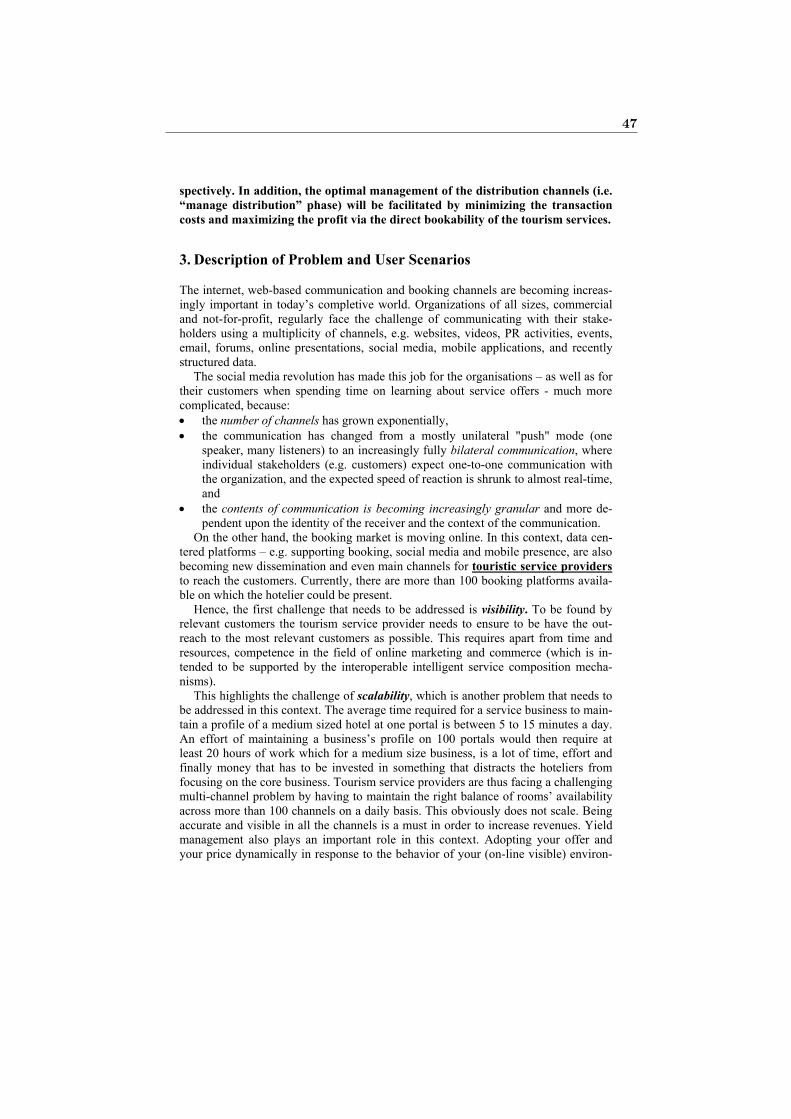
5

spectively. In addition, the optimal management of the distribution channels (i.e. “manage distribution” phase) will be facilitated by minimizing the transaction costs and maximizing the profit via the direct bookability of the tourism services.

3. Description of Problem and User Scenarios

The internet, web-based communication and booking channels are becoming increas-ingly important in today’s completive world. Organizations of all sizes, commercial and not-for-profit, regularly face the challenge of communicating with their stake-holders using a multiplicity of channels, e.g. websites, videos, PR activities, events, email, forums, online presentations, social media, mobile applications, and recently structured data.

The social media revolution has made this job for the organisations – as well as for their customers when spending time on learning about service offers - much more complicated, because: x the number of channels has grown exponentially, x the communication has changed from a mostly unilateral "push" mode (one

speaker, many listeners) to an increasingly fully bilateral communication, where individual stakeholders (e.g. customers) expect one-to-one communication with the organization, and the expected speed of reaction is shrunk to almost real-time, and

x the contents of communication is becoming increasingly granular and more de-pendent upon the identity of the receiver and the context of the communication.

On the other hand, the booking market is moving online. In this context, data cen-tered platforms – e.g. supporting booking, social media and mobile presence, are also becoming new dissemination and even main channels for touristic service providers to reach the customers. Currently, there are more than 100 booking platforms availa-ble on which the hotelier could be present.

Hence, the first challenge that needs to be addressed is visibility. To be found by relevant customers the tourism service provider needs to ensure to be have the out-reach to the most relevant customers as possible. This requires apart from time and resources, competence in the field of online marketing and commerce (which is in-tended to be supported by the interoperable intelligent service composition mecha-nisms).

This highlights the challenge of scalability, which is another problem that needs to be addressed in this context. The average time required for a service business to main-tain a profile of a medium sized hotel at one portal is between 5 to 15 minutes a day. An effort of maintaining a business’s profile on 100 portals would then require at least 20 hours of work which for a medium size business, is a lot of time, effort and finally money that has to be invested in something that distracts the hoteliers from focusing on the core business. Tourism service providers are thus facing a challenging multi-channel problem by having to maintain the right balance of rooms’ availability across more than 100 channels on a daily basis. This obviously does not scale. Being accurate and visible in all the channels is a must in order to increase revenues. Yield management also plays an important role in this context. Adopting your offer and your price dynamically in response to the behavior of your (on-line visible) environ-

47

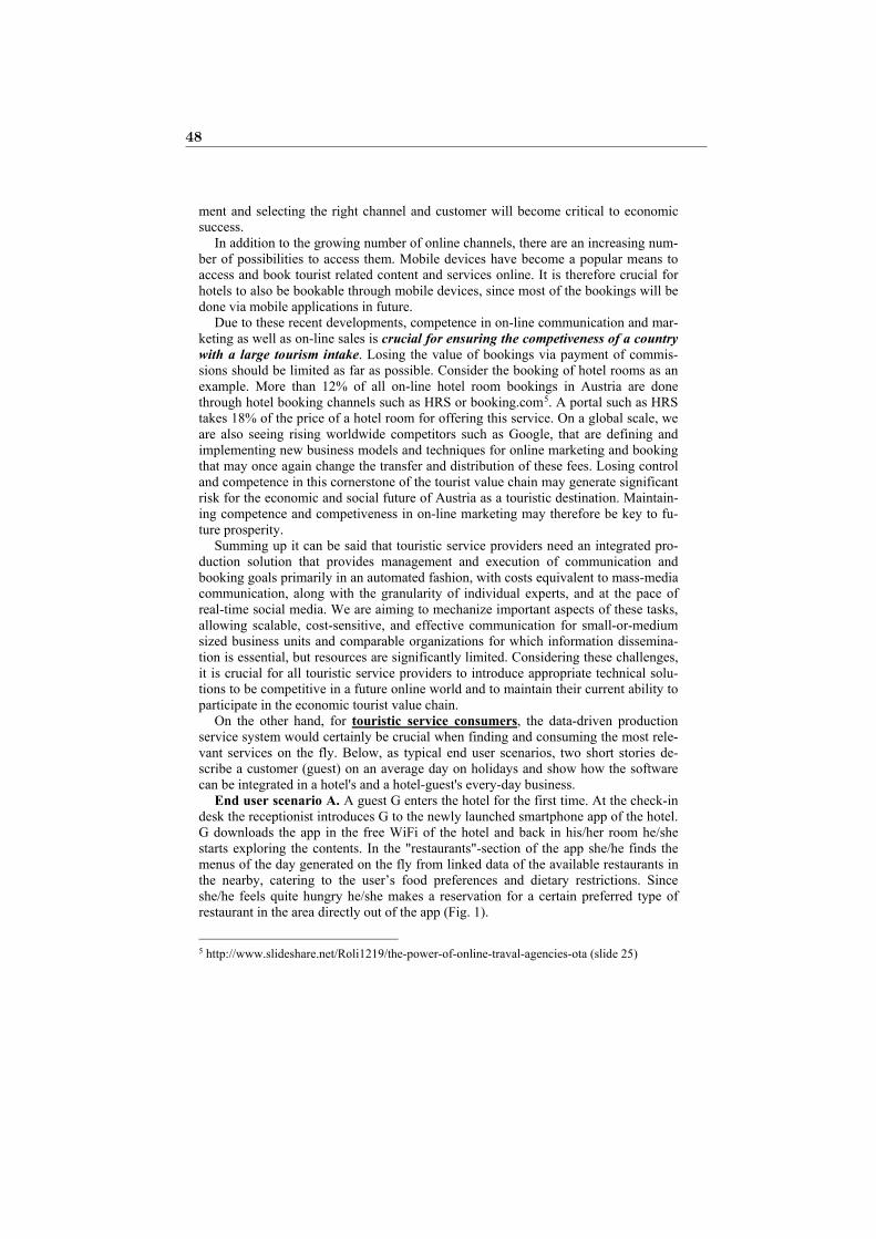
6

ment and selecting the right channel and customer will become critical to economic success.

In addition to the growing number of online channels, there are an increasing num-ber of possibilities to access them. Mobile devices have become a popular means to access and book tourist related content and services online. It is therefore crucial for hotels to also be bookable through mobile devices, since most of the bookings will be done via mobile applications in future.

Due to these recent developments, competence in on-line communication and mar-keting as well as on-line sales is crucial for ensuring the competiveness of a country with a large tourism intake. Losing the value of bookings via payment of commis-sions should be limited as far as possible. Consider the booking of hotel rooms as an example. More than 12% of all on-line hotel room bookings in Austria are done through hotel booking channels such as HRS or booking.com 4F

5. A portal such as HRS takes 18% of the price of a hotel room for offering this service. On a global scale, we are also seeing rising worldwide competitors such as Google, that are defining and implementing new business models and techniques for online marketing and booking that may once again change the transfer and distribution of these fees. Losing control and competence in this cornerstone of the tourist value chain may generate significant risk for the economic and social future of Austria as a touristic destination. Maintain-ing competence and competiveness in on-line marketing may therefore be key to fu-ture prosperity.

Summing up it can be said that touristic service providers need an integrated pro-duction solution that provides management and execution of communication and booking goals primarily in an automated fashion, with costs equivalent to mass-media communication, along with the granularity of individual experts, and at the pace of real-time social media. We are aiming to mechanize important aspects of these tasks, allowing scalable, cost-sensitive, and effective communication for small-or-medium sized business units and comparable organizations for which information dissemina-tion is essential, but resources are significantly limited. Considering these challenges, it is crucial for all touristic service providers to introduce appropriate technical solu-tions to be competitive in a future online world and to maintain their current ability to participate in the economic tourist value chain.

On the other hand, for touristic service consumers, the data-driven production service system would certainly be crucial when finding and consuming the most rele-vant services on the fly. Below, as typical end user scenarios, two short stories de-scribe a customer (guest) on an average day on holidays and show how the software can be integrated in a hotel's and a hotel-guest's every-day business.

End user scenario A. A guest G enters the hotel for the first time. At the check-in desk the receptionist introduces G to the newly launched smartphone app of the hotel. G downloads the app in the free WiFi of the hotel and back in his/her room he/she starts exploring the contents. In the "restaurants"-section of the app she/he finds the menus of the day generated on the fly from linked data of the available restaurants in the nearby, catering to the user’s food preferences and dietary restrictions. Since she/he feels quite hungry he/she makes a reservation for a certain preferred type of restaurant in the area directly out of the app (Fig. 1).

5 http://www.slideshare.net/Roli1219/the-power-of-online-traval-agencies-ota (slide 25)

48

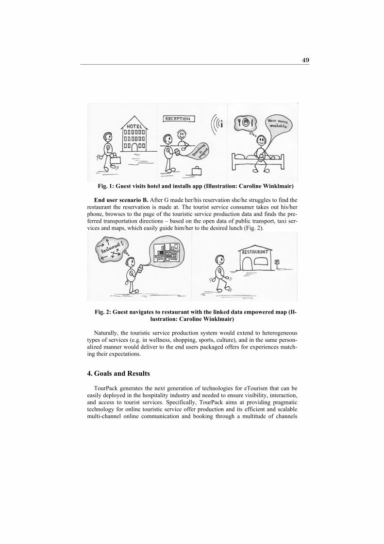
7

Fig. 1: Guest visits hotel and installs app (Illustration: Caroline Winklmair) End user scenario B. After G made her/his reservation she/he struggles to find the

restaurant the reservation is made at. The tourist service consumer takes out his/her phone, browses to the page of the touristic service production data and finds the pre-ferred transportation directions – based on the open data of public transport, taxi ser-vices and maps, which easily guide him/her to the desired lunch (Fig. 2).

Fig. 2: Guest navigates to restaurant with the linked data empowered map (Il-

lustration: Caroline Winklmair) Naturally, the touristic service production system would extend to heterogeneous

types of services (e.g. in wellness, shopping, sports, culture), and in the same person-alized manner would deliver to the end users packaged offers for experiences match-ing their expectations.

4. Goals and Results

TourPack generates the next generation of technologies for eTourism that can be easily deployed in the hospitality industry and needed to ensure visibility, interaction, and access to tourist services. Specifically, TourPack aims at providing pragmatic technology for online touristic service offer production and its efficient and scalable multi-channel online communication and booking through a multitude of channels

49

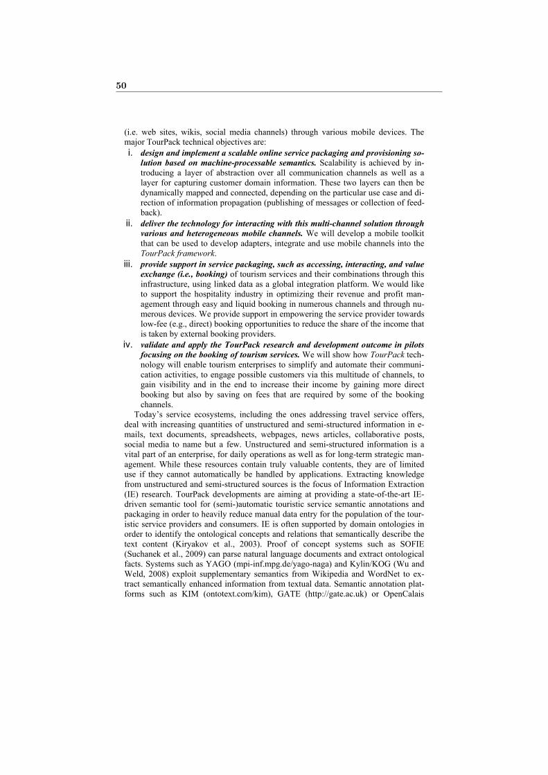
8

(i.e. web sites, wikis, social media channels) through various mobile devices. The major TourPack technical objectives are: i. design and implement a scalable online service packaging and provisioning so-

lution based on machine-processable semantics. Scalability is achieved by in-troducing a layer of abstraction over all communication channels as well as a layer for capturing customer domain information. These two layers can then be dynamically mapped and connected, depending on the particular use case and di-rection of information propagation (publishing of messages or collection of feed-back).

ii. deliver the technology for interacting with this multi-channel solution through various and heterogeneous mobile channels. We will develop a mobile toolkit that can be used to develop adapters, integrate and use mobile channels into the TourPack framework.

iii. provide support in service packaging, such as accessing, interacting, and value exchange (i.e., booking) of tourism services and their combinations through this infrastructure, using linked data as a global integration platform. We would like to support the hospitality industry in optimizing their revenue and profit man-agement through easy and liquid booking in numerous channels and through nu-merous devices. We provide support in empowering the service provider towards low-fee (e.g., direct) booking opportunities to reduce the share of the income that is taken by external booking providers.

iv. validate and apply the TourPack research and development outcome in pilots focusing on the booking of tourism services. We will show how TourPack tech-nology will enable tourism enterprises to simplify and automate their communi-cation activities, to engage possible customers via this multitude of channels, to gain visibility and in the end to increase their income by gaining more direct booking but also by saving on fees that are required by some of the booking channels.

Today’s service ecosystems, including the ones addressing travel service offers, deal with increasing quantities of unstructured and semi-structured information in e-mails, text documents, spreadsheets, webpages, news articles, collaborative posts, social media to name but a few. Unstructured and semi-structured information is a vital part of an enterprise, for daily operations as well as for long-term strategic man-agement. While these resources contain truly valuable contents, they are of limited use if they cannot automatically be handled by applications. Extracting knowledge from unstructured and semi-structured sources is the focus of Information Extraction (IE) research. TourPack developments are aiming at providing a state-of-the-art IE-driven semantic tool for (semi-)automatic touristic service semantic annotations and packaging in order to heavily reduce manual data entry for the population of the tour-istic service providers and consumers. IE is often supported by domain ontologies in order to identify the ontological concepts and relations that semantically describe the text content (Kiryakov et al., 2003). Proof of concept systems such as SOFIE (Suchanek et al., 2009) can parse natural language documents and extract ontological facts. Systems such as YAGO (mpi-inf.mpg.de/yago-naga) and Kylin/KOG (Wu and Weld, 2008) exploit supplementary semantics from Wikipedia and WordNet to ex-tract semantically enhanced information from textual data. Semantic annotation plat-forms such as KIM (ontotext.com/kim), GATE (http://gate.ac.uk) or OpenCalais

50

9

(http://www.opencalais.com) locate and extract entities, relationships, and facts in texts, and create semantic links between different documents, data, domain models, and Linked Data. Once extracted from various sources, relevant manufacturing eco-system knowledge can be inter-linked and then clustered in order to enable better search and navigation of virtual artefacts. This can be realized using approaches and techniques such as those provided by LarKC (larkc.eu) or LOD2 (lod2.eu). LarKC developed methods and tools to recognize entities and relations, and to interlink these entities with existing documents to provide richer search experiences. LOD2 support-ed Sindice (sindice.com), a platform for building applications on top of RDF-based Linked Data.

We will support automatic generation, clustering and packaging of semantically annotated touristic service offers from a variety of sources. More precisely, existing information extraction, clustering and publishing will be adopted and extended in order to: x obtain the extracted data in a Linked Data format, (semi-)automatically associat-

ing metadata; x generate service representations in Linked Data format according to ontological

models; x interlink, cluster, package and provide services in an automatic way; x provide a semantic service and an online interface for easy publishing and access

to the above mentioned functionalities. As confirmed by the industry partners involved in this proposal, costs remain the

main decisive factor for SME adoption of innovative ICT solutions. We plan to build upon open source tools for information extraction, interlinking and clustering many of the ones mentioned above. In particular we will consider OpenCalais for information extraction as well as linking and clustering tools developed by LarKC and LOD2 projects.

Further, the TourPack approach addresses a number of innovative challenges, and expected technical outcome and own contributions of the project are summarized in the following table:

Challenge Outcome

Multi-channel communica-tion see (Fensel et al., 2012), (Toma et al., 2013), (Fensel et al., 2014)

x Semantic based representation of content (on-tology) in intuitive and familiar terminology for tourist service providers.

x Scalable methods for separating and interweaving content and communication channels, particularly, employing linked data as an integration platform.

x Online multi-channel communication technical solution.

Online interactions see (Fensel et al., 2014), (Stavrakantonakis et al., 2014-1)

x Formal communication pattern description mechanism as business processes.

x Reusable set of communication patterns to structure the online interactions for the tourism domain.

51

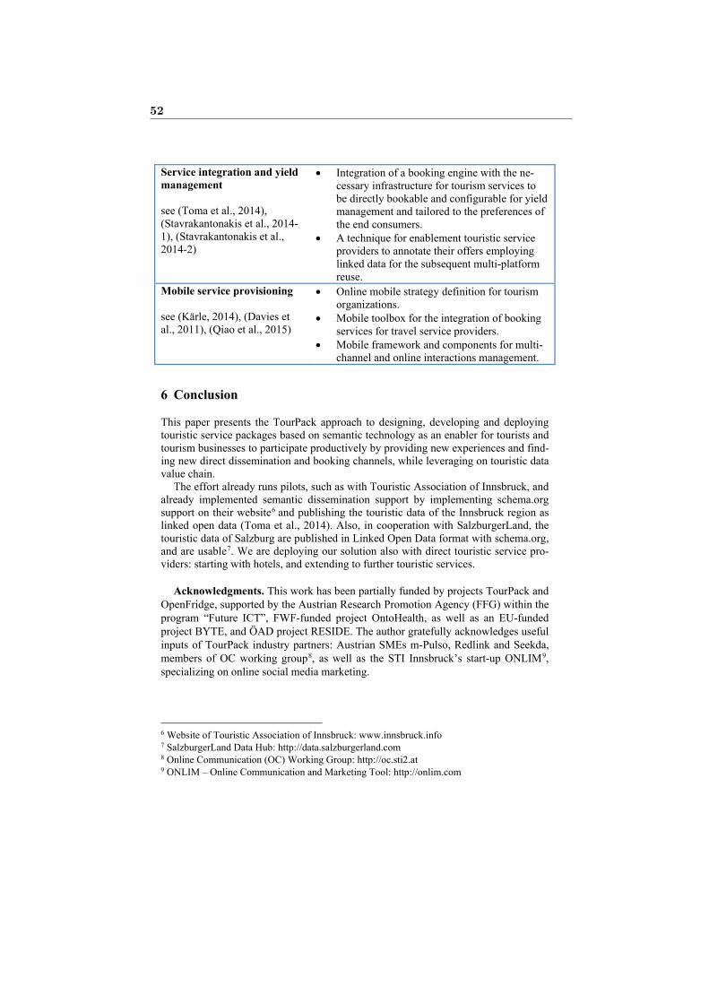
10

Service integration and yield management see (Toma et al., 2014), (Stavrakantonakis et al., 2014-1), (Stavrakantonakis et al., 2014-2)

x Integration of a booking engine with the ne-cessary infrastructure for tourism services to be directly bookable and configurable for yield management and tailored to the preferences of the end consumers.

x A technique for enablement touristic service providers to annotate their offers employing linked data for the subsequent multi-platform reuse.

Mobile service provisioning see (Kärle, 2014), (Davies et al., 2011), (Qiao et al., 2015)

x Online mobile strategy definition for tourism organizations.

x Mobile toolbox for the integration of booking services for travel service providers.

x Mobile framework and components for multi-channel and online interactions management.

6 Conclusion

This paper presents the TourPack approach to designing, developing and deploying touristic service packages based on semantic technology as an enabler for tourists and tourism businesses to participate productively by providing new experiences and find-ing new direct dissemination and booking channels, while leveraging on touristic data value chain.

The effort already runs pilots, such as with Touristic Association of Innsbruck, and already implemented semantic dissemination support by implementing schema.org support on their website5F

6 and publishing the touristic data of the Innsbruck region as linked open data (Toma et al., 2014). Also, in cooperation with SalzburgerLand, the touristic data of Salzburg are published in Linked Open Data format with schema.org, and are usable6F

7. We are deploying our solution also with direct touristic service pro-viders: starting with hotels, and extending to further touristic services.

Acknowledgments. This work has been partially funded by projects TourPack and OpenFridge, supported by the Austrian Research Promotion Agency (FFG) within the program “Future ICT”, FWF-funded project OntoHealth, as well as an EU-funded project BYTE, and ÖAD project RESIDE. The author gratefully acknowledges useful inputs of TourPack industry partners: Austrian SMEs m-Pulso, Redlink and Seekda, members of OC working group7F

8, as well as the STI Innsbruck’s start-up ONLIM 8F

9, specializing on online social media marketing.

6 Website of Touristic Association of Innsbruck: www.innsbruck.info 7 SalzburgerLand Data Hub: http://data.salzburgerland.com 8 Online Communication (OC) Working Group: http://oc.sti2.at 9 ONLIM – Online Communication and Marketing Tool: http://onlim.com

52

11

References

Revinate. (2012). Using Social Media and Mobile to Improve Guest Satisfaction - The Revinate Blog. Retrieved from http://blog.revinate.com/2012/09/using-social-media-and-mobile-to-improve-guest-satisfaction.html

Google (2012). “What Users Want Most From Mobile Sites Today”. Google survey con-ducted by Sterling Research and Smith Geiger, July 2012. Retrieved from: http://www.thinkwithgoogle.com/insights/library/studies/what-users-want-most-from-mobile-sites-today/

Gaffney, A.: Improving Customer Satisfaction Through More Effective ICT Strategies. Vol. 1, pp. 1–7, 2007.

Hayes, D.K., and Miller, A.A.: Revenue Management for the Hospitality Industry. Book, Wiley 2010.

Xylander, J.K.: Kapazitätsmanagement Bei Reiseveranstaltern: Entscheidungsmodelle Zur Kontingentierung Im Yield Management. Deutscher Universitätsverlag, 2003.

Fandel, G.: Revenue Management. ZfB Special Issue 1/2005, Gabler. Amersdorffer, D., Bauhuber, F., Egger, R., and Oellrich, J.: Social Web im Tourismus.

Springer, 2010. Weiß, M., Haüßler, S.: Yield Management – Konzepte und Techniken. Grin, 2005. Gannod, G.C., Zhu, H. and Mudiam, S.V.: On-the-fly Wrapping of Web Services to Support

Dynamic Integration. In Proceedings of the 10th Working Conference on Reverse Engineering (WCRE '03). IEEE Computer Society, Washington, DC, USA, 175-184, 2003.

Leong, H.W., Brutzman, D., McGregor, D. and Blais, C.: Web services integration on the fly for service-oriented computing and simulation. In Proceedings of the 2009 Spring Simula-tion Multiconference (SpringSim '09). Society for Computer Simulation International, San Diego, CA, USA, Article 40 , 8 pages, 2009.

N. Ibrahim, F. Le Mouël, and S. Frénot: MySIM: a spontaneous service integration middle-ware for pervasive environments. In Proceedings of the 2009 international conference on Per-vasive services (ICPS '09). ACM, New York, NY, USA, 1-10, 2009.

Kiryakov, A., Popov, B., Terziev, I., Manov, D. and Ognyanoff, D. (2003) Semantic Anno-tation, Indexing, and Retrieval, In Proceedings of the 2nd International Semantic Web Confer-ence (ISWC 2003), pp.49–79.

Suchanek, F. M., Sozio, M. and Weikum, G. (2009), SOFIE: A Self-Organizing Framework for Information Extraction, in Proceedings of WWW 2009, Madrid.

Wu, F., and Weld, D. (2008) Automatically refining the Wikipedia infobox ontology, in Proc. of WWW 2008, Beijing.

Fensel, A., Fensel, D., Leiter, B., Thalhammer, A. " Effective and Efficient Online Commu-nication: The Channel Model". In Proceedings of International Conference on Data Technolo-gies and Applications (DATA’12), pp. 209-215, SciTePress, Rome, Italy, 25-27 July, 2012.

Toma, I., Fensel, D., Gagiu, A.-E., Stavrakantonakis, I., Fensel, A., Leiter, B., Thalhammer, A., Larizgoitia, I., Garcia, J.-M. "Enabling Scalable Multi-Channel Communication through Semantic Technologies". In Proceedings of the IEEE/WIC/ACM International Conference on Web Intelligence, November 17-20, 2013, Atlanta, USA, IEEE Computer Society Press (2013).

Toma, I., Stanciu, C.-V., Fensel, A., Stavrakantonakis, I., Fensel, D. "Improving the online visibility of touristic service providers by using semantic annotations". In Proceedings of the 11th European Semantic Web Conference (ESWC'2014) – Poster and Demo Track, 25-29 May 2014, Crete, Greece, Springer-Verlag, LNCS (2014).

Stavrakantonakis, I., Fensel, A., Fensel, D. "Matching Web Entities with Potential Actions", In Proceedings of the Poster Paper track International Conference on Semantic Systems (I-SEMANTICS’14), CEUR-WS Vol. 1224, 4-5 September 2014, Leipzig, Germany (2014).

Stavrakantonakis, I., Toma, I., Fensel, A., Fensel, D. “Hotel Websites, Web 2.0, Web 3.0 and Online Direct Marketing: The Case of Austria”. In Proceedings of the 21th International

53

12

Conference on Information and Communication Technologies in Travel and Tourism (ENTER2014), pp. 665-677, 21-24 January 2014, Dublin, Ireland, Springer (2014).

Kärle, E. Master thesis “An approach and implementation for supporting multi-platform mobile service creation for businesses”, January 2014, University of Innsbruck, Austria.

Davies, M., Carrez, F., Heinilä, J., Fensel, A., Narganes, M., Danado, J. "m:Ciudad -- Ena-bling End-User Mobile Service Creation", International Journal of Pervasive Computing and Communications, Emerald Group Publishing, Vol. 7 Iss: 4, pp. 384-414 (2011).

Qiao, X., Xue, S., Chen, J., Fensel, A. “A Lightweight Convergent Personal Mobile Service Delivery Approach Based on Phone Book”. International Journal of Communication Systems, Vol. 28 Iss: 1, pp. 49-70, Wiley, January 2015.

54

A Practical Framework for RelBACImplementation

Lei Liu1, Quanzhu Tao1, Fausto Giunchiglia2 and Rui Zhang1?

1 CCST, Jilin University, Str. Qianjin 2699, Changchun, China 130012liulei@jlu.edu.cn

tqzlimit@126.com

rui@jlu.edu.cn2 DISI, University of Trento, Italy

fausto@disi.unitn.it

Abstract. RelBAC is a new access control model that has graduallyaroused the research interest in the domain of access control. But it isstill not mature enough for industrial application due to its high logicalcomplexity. In this paper, we present a framework to implement Rel-BAC . First, access control queries to RelBAC knowledge base (KB) areanalysed and categorized into different queries as run-time or off-line.Then the necessary knowledge is studied to answer each type of query.We propose to separate the knowledge for run-time query, named as acomplete ABox, from the classical RelBAC KB and store it in a relation-al database, so as to provide run-time answers within acceptable time.Last, a theorem is proved to backbone our method and an algorithm isproposed to calculate the complete ABox. This framework serves as ameaningful attempt to put RelBAC into practice.

Keywords: RelBAC , Description Logic, Complete ABox

1 Introduction

Access control models evolute with the advances of technologies. The famousRole-based Access Control model RBAC [4] was proposed in the 20th century,has now flourished in practical access control systems such as in Windows oper-ation systems. It evolves into different models such as ARBAC [11], GeoRBAC[3], ARBAC [8] etc.

As a new access control model, RelBAC [6] connects the subject that query toaccess the object with the permission as a binary relation. The model providesintuitive and straightforward semantics to home users without formal accesscontrol experiences. But RelBAC has not flourished as expected in industrysolutions. What hinders the model from practical application is the shortageof background supporting mechanism, which is supposed to be the powerfulreasoning services provided by description logic (DL) reasoners. There is nogood enough general purpose reasoners for RelBAC yet.

? Corresponding Author

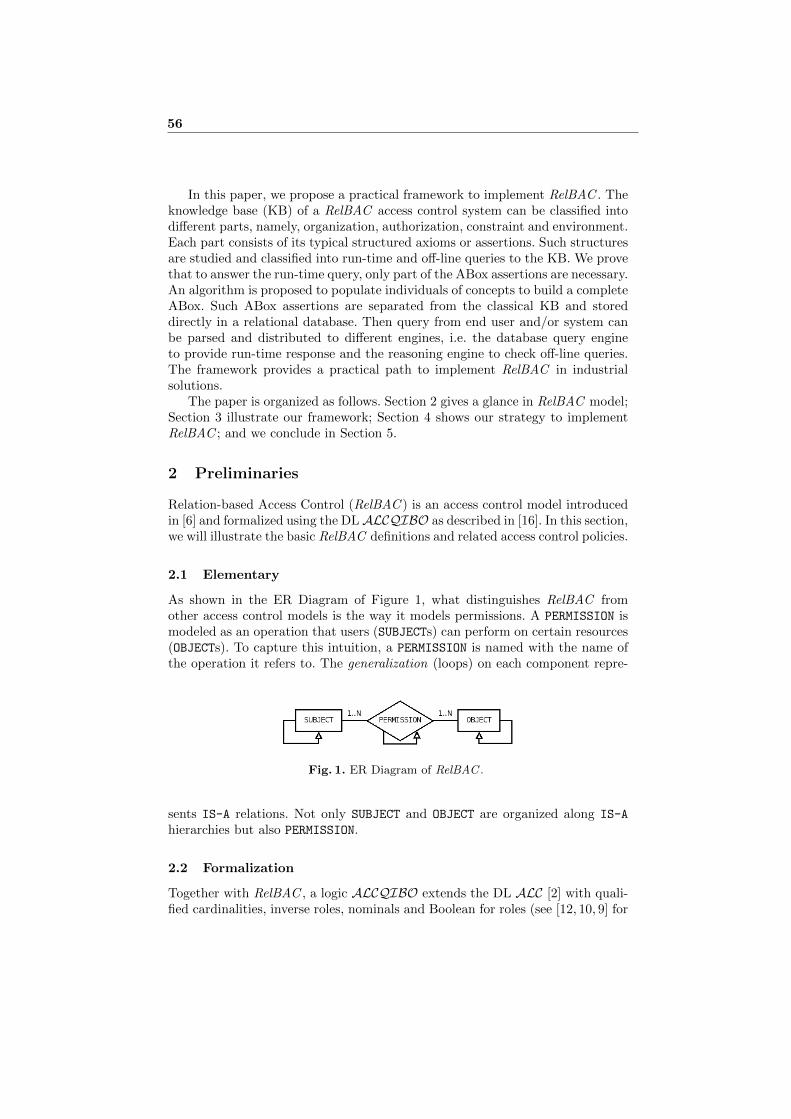
In this paper, we propose a practical framework to implement RelBAC . Theknowledge base (KB) of a RelBAC access control system can be classified intodifferent parts, namely, organization, authorization, constraint and environment.Each part consists of its typical structured axioms or assertions. Such structuresare studied and classified into run-time and off-line queries to the KB. We provethat to answer the run-time query, only part of the ABox assertions are necessary.An algorithm is proposed to populate individuals of concepts to build a completeABox. Such ABox assertions are separated from the classical KB and storeddirectly in a relational database. Then query from end user and/or system canbe parsed and distributed to different engines, i.e. the database query engineto provide run-time response and the reasoning engine to check off-line queries.The framework provides a practical path to implement RelBAC in industrialsolutions.

The paper is organized as follows. Section 2 gives a glance in RelBAC model;Section 3 illustrate our framework; Section 4 shows our strategy to implementRelBAC ; and we conclude in Section 5.

2 Preliminaries

Relation-based Access Control (RelBAC ) is an access control model introducedin [6] and formalized using the DLALCQIBO as described in [16]. In this section,we will illustrate the basic RelBAC definitions and related access control policies.

2.1 Elementary

As shown in the ER Diagram of Figure 1, what distinguishes RelBAC fromother access control models is the way it models permissions. A PERMISSION ismodeled as an operation that users (SUBJECTs) can perform on certain resources(OBJECTs). To capture this intuition, a PERMISSION is named with the name ofthe operation it refers to. The generalization (loops) on each component repre-

Fig. 1. ER Diagram of RelBAC .

sents IS-A relations. Not only SUBJECT and OBJECT are organized along IS-A

hierarchies but also PERMISSION.

2.2 Formalization

Together with RelBAC , a logic ALCQIBO extends the DL ALC [2] with quali-fied cardinalities, inverse roles, nominals and Boolean for roles (see [12, 10, 9] for

56

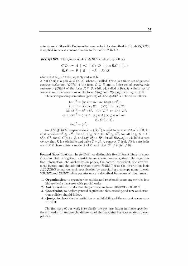
extensions of DLs with Booleans between roles). As described in [1], ALCQIBOis applied in access control domain to formalize RelBAC .

ALCQIBO. The syntax of ALCQIBO is defined as follows.

C,D ::= A | ¬C | C uD | ≥ nR.C | {ai}R,S ::= P | R− | ¬R | R u S

where A ∈ NC, P ∈ NR, ai ∈ NI and n ∈ N.A KB (KB) is a pair K = 〈T ,A〉 where T , called TBox, is a finite set of generalconcept inclusions (GCIs) of the form C v D and a finite set of general roleinclusions (GRIs) of the form R v S, while A, called ABox, is a finite set ofconcept and role assertions of the form C(ai) and R(ai, aj), with ai, aj ∈ NI.

The corresponding semantics (partial) of ALCQIBO is defined as follows.

(R−)I := {(y, x) ∈ ∆×∆ | (x, y) ∈ RI},(¬R)I := ∆×∆ \RI , (¬C)I := ∆ \ CI ,

(R u S)I := RI ∩ SI , (C uD)I := CI ∩DI ,(> n R.C)I := {x ∈ ∆ | ]{y ∈ ∆ | (x, y) ∈ RI and

y ∈ CI} ≥ n},{ai}I := {aIi }.

An ALCQIBO-interpretation I = (∆, ·I) is said to be a model of a KB, K,iff it satisfies CI ⊆ DI , for all C v D ∈ K, RI ⊆ SI , for all R v S ∈ K,aIi ∈ CI , for all C(ai) ∈ A, and (aIi , a

Ij ) ∈ RI , for all R(ai, aj) ∈ A. In this case

we say that K is satisfiable and write I |= K. A concept C (role R) is satisfiablew.r.t. K if there exists a model I of K such that CI 6= ∅ (RI 6= ∅).

Formal Specification. In RelBAC we distinguish five different kinds of spec-ifications that, altogether, constitute an access control system: the organiza-tion information, the authorization policy, the control constraint, the environ-ment factors and the administration query. RelBAC uses the description logicALCQIBO to express each specification by associating a concept name to eachSUBJECT and OBJECT while permissions are described by means of role names.

1. Organization, to organize the entities and relationships among entities intohierarchical structures with partial order.

2. Authorization, to declare the permissions from SUBJECT to OBJECT.3. Constraint, to declare general regulations that existing and new authoriza-

tion policies should follow.4. Query, to check the instantiation or satisfiability of the current access con-

trol KB.

The first step of our work is to clarify the patterns latent in above specifica-tions in order to analyze the difference of the reasoning services related to eachpattern.

57

3 Framework

Based on the theory of RelBAC , we propose a framework towards the imple-mentation of the theory. It consists of three layers coherent to a standard MVCstructure, but specialized to fit the access control domain.

Figure 2 gives the conceptual model of the frame.

Fig. 2. Conceptual model of the frame for RelBAC Model.

As is shown in the figure, the framework consists of three major components,interface, engine and KB. Let us get into the details of them one by one.

Interface It is the intermediate between the system internal components andthe outer ‘users’. A channel, predefined or constructed at runtime, serversas interface is maintained by this component. It is not bounded to classicaluser interface but provides three sub components, SI, AI and UI.

SI It stands for System Interface, which communicates with the outer in-formation providers, such as time server, behavior monitor, audit recordserver, etc. Environment information are mainly transmitted to the sys-tem through SI.

AI It stands for Administrative Interface, which connects administrators tothe system via predefined graphical interfaces and facilitate tool inter-faces.

UI It stands for Usser Interface, that provides classical graphical interfacesto end users. AI pages could be reused for UI, only with appropriateaccess control.

Engine It is the core part of the frame, that processes the info (updates, queries,maintenance, etc.) and communicate (if needed) with the KB. It mainlyconsists of three sub engines, PE, RE and QE.

PE It is the Parser Engine, which will preprocess the information from theinterface, and forward it to appropriate engines for further processes.Different type of system queries will arrive, and fit in predefined or run-time studied patterns, then re-formulated into processable intermediate

58

format, thereafter be sent to responsible engines. Details of the formatsand patterns will be discussed in Section 4.

RE It is the Reasoning Engine, that accepts OWL-API format reasoningtasks and provides reasoning services together with the interaction withthe ontology KB(s).

QE It is the Query Engine that takes the database queries as input andprovides necessary query answers via access to the database in the KB.

KB It stores the knowledge necessary for the access control system function-ality, such as the organization of the SUBJECT, OBJECT and PERMISSION;the authorization and constraint policies; the environment factors, etc. Itis divided into two parts, the AK and DK, which stores the knowledge fordifferent purposes.AK It is the Administrative Knowledge base, aims at general policies that

support the administrative queries. It usually interacts with RE as thereasoning background.

CK It is the Control Knowledge implemented via classical relational databasetechniques. Instantiated knowledge, such as the ABox assertion that‘John is permitted to update the root path’ is stored here.

With the framework, the next step is to work out the details of each compo-nent. We will describe the theoretical details in the next section.

4 Implementation

This section will focus on the theoretical aspects to implement the frameworkintroduced above. The patterns are clarified for the knowledge in a RelBACsystem. Then the distribution strategy is proposed in details.

4.1 Knowledge Pattern

One of the key issue to implement the framework is to clarify the possible knowl-edge patterns. In Section 2.2, knowledge has been classified into four categories.Here, we will identify the patterns from the categories.

1. Organization: In the access control terminology, SUBJECT, OBJECT andPERMISSION may be organized in a taxonomy along the IS-A relation [5].An IS-A relation is represented as a concept (or role) inclusion axiom inRelBAC :

C v D or P v Q (1)

where C,D are both SUBJECTs or both OBJECTs; P,Q are both PERMISSIONs.SUBJECT and OBJECT are easy to be organized into IS-A hierarchies, espe-cially with concerned attributes. Besides, compound concepts constructedwith classical DL operator ¬ and u may also exist in the formula above. Theinversion operator − on role may also join in the inclusion axiom of roles inFormula (1).

59

Moreover, in addition to the DL roles for PERMISSION, classical roles may alsoexist to describe binary relations between entities that is not a PERMISSION,such as ‘is-older-than’ or ‘has-published’ relation in a system with an aca-demic background. The inverse role operator

The number restriction operator ≥ is seldom used in organization. Its com-bination with the other operators will results in an axiom that could not beinstantiated, as it puts restrictions on cardinality rather than fix individuals.This is more likely to be used in the specification of constraints.

2. Authorization: It specifies a permission existing between a SUBJECT andan OBJECT both on organization level or instance level in various of forms.

S v ∀¬P.¬O or O v ∀¬P−.¬S (2)

which specifies that any SUBJECT in S is permitted to perform the operation(with the same name) P on any OBJECT in O. For easy reading purpose, itis transformed into a SWRL [14] rule as

S(?x), O(?y)→ P (?x, ?y) (2′)

Special cases exist for Formula (2′), with alternation of the concept(s) withnominal(s), we have the following variations.

{..., si, ...} v ∀¬P.¬OS v ∀¬P.¬{..., oj , ...}

{..., si, ...} v ∀¬P.¬{..., oj , ...} (2′′)

where i, j are natural number indexes for individuals of SUBJECT and OBJECT.An authorization policy in the form of an ABox assertion P (s, o) is only aspecial case of Formula (2′′).

3. Constraint: It specifies the restrictions or regulations that the authorizationpolicies should not violate. A constraint usually stays inactive in a runningsystem. But when environment factors change, such as the rise of the systemload, the crucial time point, the access behavior violation, etc. Therefore, thereasoning engine should check the consistency of the KB when new knowl-edge arrives or current knowledge updates.

Some of the most concerned constraints are:

(a) Separation of Duties (SoD): It regulates the mutual exclusivenessof permissions. SoD lies in different levels and granularity. Given a setof positions S = {S1, . . . , Sn}, where each Si is a concept name, a SoDpolicy ‘a subject can take all the positions in S’, may take the form ofan unsatisfiable compound role (in contrast to an atomic role).

Cmn⊔

i=1

(

ml

j=1

Sij ) v ⊥ (3)

60

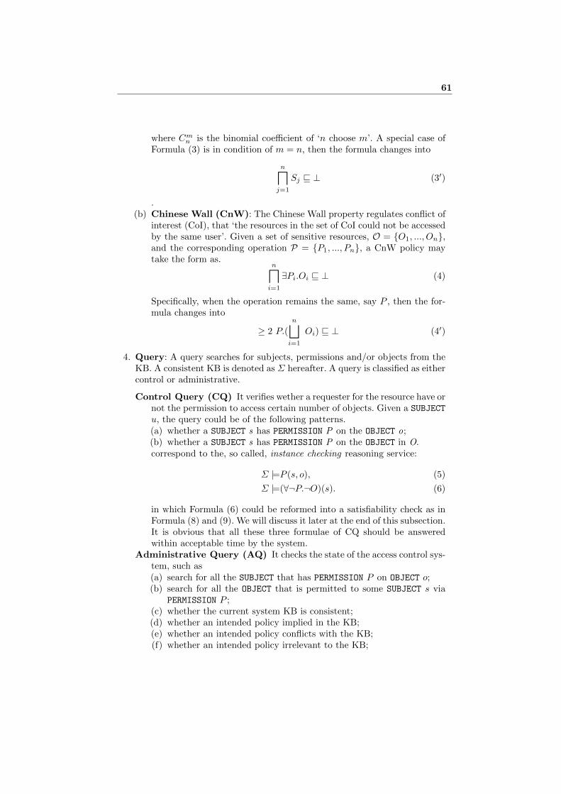
where Cmn is the binomial coefficient of ‘n choose m’. A special case of

Formula (3) is in condition of m = n, then the formula changes into

nl

j=1

Sj v ⊥ (3′)

.(b) Chinese Wall (CnW): The Chinese Wall property regulates conflict of

interest (CoI), that ‘the resources in the set of CoI could not be accessedby the same user’. Given a set of sensitive resources, O = {O1, ..., On},and the corresponding operation P = {P1, ..., Pn}, a CnW policy maytake the form as.

nl

i=1

∃Pi.Oi v ⊥ (4)

Specifically, when the operation remains the same, say P , then the for-mula changes into

≥ 2 P.(

n⊔

i=1

Oi) v ⊥ (4′)

4. Query: A query searches for subjects, permissions and/or objects from theKB. A consistent KB is denoted as Σ hereafter. A query is classified as eithercontrol or administrative.

Control Query (CQ) It verifies wether a requester for the resource have ornot the permission to access certain number of objects. Given a SUBJECT

u, the query could be of the following patterns.(a) whether a SUBJECT s has PERMISSION P on the OBJECT o;(b) whether a SUBJECT s has PERMISSION P on the OBJECT in O.correspond to the, so called, instance checking reasoning service:

Σ |=P (s, o), (5)

Σ |=(∀¬P.¬O)(s). (6)

in which Formula (6) could be reformed into a satisfiability check as inFormula (8) and (9). We will discuss it later at the end of this subsection.It is obvious that all these three formulae of CQ should be answeredwithin acceptable time by the system.

Administrative Query (AQ) It checks the state of the access control sys-tem, such as(a) search for all the SUBJECT that has PERMISSION P on OBJECT o;(b) search for all the OBJECT that is permitted to some SUBJECT s via

PERMISSION P ;(c) whether the current system KB is consistent;(d) whether an intended policy implied in the KB;(e) whether an intended policy conflicts with the KB;(f) whether an intended policy irrelevant to the KB;

61

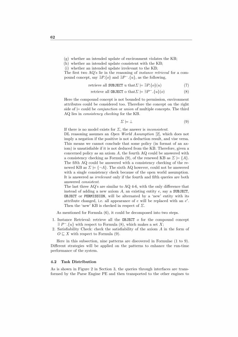
(g) whether an intended update of environment violates the KB;(h) whether an intended update consistent with the KB;(i) whether an intended update irrelevant to the KB;The first two AQ’s lie in the reasoning of instance retrieval for a com-pound concept, say ∃P.{o} and ∃P−.{u}, as the following,

retrieve all SUBJECT u thatΣ |= ∃P.{o}(u) (7)

retrieve all OBJECT o thatΣ |= ∃P−.{u}(o) (8)

Here the compound concept is not bounded to permission, environmentattributes could be considered too. Therefore the concept on the rightside of |= could be conjunction or union of multiple concepts. The thirdAQ lies in consistency checking for the KB.

Σ |= ⊥ (9)

If there is no model exists for Σ, the answer is inconsistent.DL reasoning assumes an Open World Assumption [2], which does notimply a negation if the positive is not a deduction result, and vise versa.This means we cannot conclude that some policy (in format of an ax-iom) is unsatisfiable if it is not deduced from the KB. Therefore, given aconcerned policy as an axiom A, the fourth AQ could be answered witha consistency checking as Formula (9), of the renewed KB as Σ |= {A}.The fifth AQ could be answered with a consistency checking of the re-newed KB as Σ |= {¬A}. The sixth AQ however, could not be answeredwith a single consistency check because of the open world assumption.It is answered as irrelevant only if the fourth and fifth queries are bothanswered consistent.The last three AQ’s are similar to AQ 4-6, with the only difference thatinstead of adding a new axiom A, an existing entity e, say a SUBJECT,OBJECT or PERMISSION, will be alternated by a ‘new’ entity with itsattribute changed, i.e. all appearance of e will be replaced with an e′.Then the ‘new’ KB is checked in respect of Σ.

As mentioned for Formula (6), it could be decomposed into two steps.

1. Instance Retrieval: retrieve all the OBJECT o for the compound concept∃ P−.{u} with respect to Formula (8), which makes a set X;

2. Satisfiability Check: check the satisfiability of the axiom A in the form ofO v X with respect to Formula (9).

Here in this subsection, nine patterns are discovered in Formulae (1 to 9).Different strategies will be applied on the patterns to enhance the run-timeperformance of the system.

4.2 Task Distribution

As is shown in Figure 2 in Section 3, the queries through interfaces are trans-formed by the Parse Engine PE and then transported to the other engines to

62

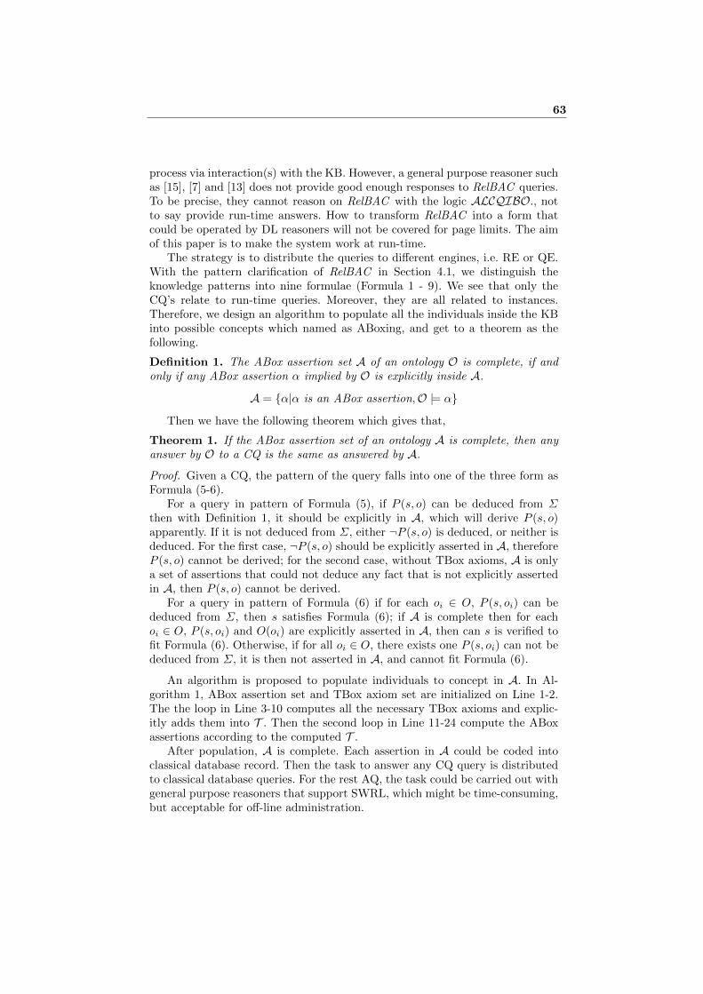
process via interaction(s) with the KB. However, a general purpose reasoner suchas [15], [7] and [13] does not provide good enough responses to RelBAC queries.To be precise, they cannot reason on RelBAC with the logic ALCQIBO., notto say provide run-time answers. How to transform RelBAC into a form thatcould be operated by DL reasoners will not be covered for page limits. The aimof this paper is to make the system work at run-time.

The strategy is to distribute the queries to different engines, i.e. RE or QE.With the pattern clarification of RelBAC in Section 4.1, we distinguish theknowledge patterns into nine formulae (Formula 1 - 9). We see that only theCQ’s relate to run-time queries. Moreover, they are all related to instances.Therefore, we design an algorithm to populate all the individuals inside the KBinto possible concepts which named as ABoxing, and get to a theorem as thefollowing.

Definition 1. The ABox assertion set A of an ontology O is complete, if andonly if any ABox assertion α implied by O is explicitly inside A.

A = {α|α is an ABox assertion,O |= α}Then we have the following theorem which gives that,

Theorem 1. If the ABox assertion set of an ontology A is complete, then anyanswer by O to a CQ is the same as answered by A.

Proof. Given a CQ, the pattern of the query falls into one of the three form asFormula (5-6).

For a query in pattern of Formula (5), if P (s, o) can be deduced from Σthen with Definition 1, it should be explicitly in A, which will derive P (s, o)apparently. If it is not deduced from Σ, either ¬P (s, o) is deduced, or neither isdeduced. For the first case, ¬P (s, o) should be explicitly asserted in A, thereforeP (s, o) cannot be derived; for the second case, without TBox axioms, A is onlya set of assertions that could not deduce any fact that is not explicitly assertedin A, then P (s, o) cannot be derived.

For a query in pattern of Formula (6) if for each oi ∈ O, P (s, oi) can bededuced from Σ, then s satisfies Formula (6); if A is complete then for eachoi ∈ O, P (s, oi) and O(oi) are explicitly asserted in A, then can s is verified tofit Formula (6). Otherwise, if for all oi ∈ O, there exists one P (s, oi) can not bededuced from Σ, it is then not asserted in A, and cannot fit Formula (6).

An algorithm is proposed to populate individuals to concept in A. In Al-gorithm 1, ABox assertion set and TBox axiom set are initialized on Line 1-2.The the loop in Line 3-10 computes all the necessary TBox axioms and explic-itly adds them into T . Then the second loop in Line 11-24 compute the ABoxassertions according to the computed T .

After population, A is complete. Each assertion in A could be coded intoclassical database record. Then the task to answer any CQ query is distributedto classical database queries. For the rest AQ, the task could be carried out withgeneral purpose reasoners that support SWRL, which might be time-consuming,but acceptable for off-line administration.

63

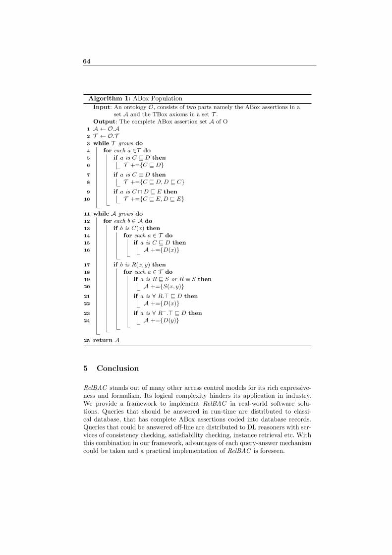
Algorithm 1: ABox Population

Input: An ontology O, consists of two parts namely the ABox assertions in aset A and the TBox axioms in a set T .

Output: The complete ABox assertion set A of O1 A ← O.A2 T ← O.T3 while T grows do4 for each a ∈T do5 if a is C v D then6 T +={C v D}7 if a is C ≡ D then8 T +={C v D,D v C}9 if a is C uD v E then

10 T +={C v E,D v E}

11 while A grows do12 for each b ∈ A do13 if b is C(x) then14 for each a ∈ T do15 if a is C v D then16 A +={D(x)}

17 if b is R(x, y) then18 for each a ∈ T do19 if a is R v S or R ≡ S then20 A +={S(x, y)}21 if a is ∀ R.> v D then22 A +={D(x)}23 if a is ∀ R−.> v D then24 A +={D(y)}

25 return A

5 Conclusion

RelBAC stands out of many other access control models for its rich expressive-ness and formalism. Its logical complexity hinders its application in industry.We provide a framework to implement RelBAC in real-world software solu-tions. Queries that should be answered in run-time are distributed to classi-cal database, that has complete ABox assertions coded into database records.Queries that could be answered off-line are distributed to DL reasoners with ser-vices of consistency checking, satisfiability checking, instance retrieval etc. Withthis combination in our framework, advantages of each query-answer mechanismcould be taken and a practical implementation of RelBAC is foreseen.

64

References

1. Artale, A., Crispo, B., Giunchiglia, F., Turkmen, F., Zhang, R.: Reasoning aboutrelation based access control. In: Xiang, Y., Samarati, P., Hu, J., Zhou, W.,Sadeghi, A.R. (eds.) NSS. pp. 231–238. IEEE Computer Society (2010)

2. Baader, F., Calvanese, D., McGuinness, D.L., Nardi, D., Patel-Schneider, P.F.(eds.): The description logic handbook: theory, implementation, and applications.Cambridge University Press, New York, NY, USA (2003)

3. Damiani, M.L., Bertino, E., Catania, B., Perlasca, P.: Geo-rbac: A spatially awarerbac. ACM Transactions on Information and System Security 10(1) (2007)

4. Ferraiolo, D.F., Cugini, J.A., Kuhn, D.R.: Role-Based Access Control (RBAC):Features and Motivations. In: 11th Annual Computer Security Applications Pro-ceedings (1995)

5. Giunchiglia, F., Zaihrayeu, I.: Lightweight ontologies. In: Encyclopedia of DatabaseSystems. Springer (2008)

6. Giunchiglia, F., Zhang, R., Crispo, B.: Relbac: Relation based access control. In:SKG ’08: Proceedings of the 2008 Fourth International Conference on Semantics,Knowledge and Grid. pp. 3–11. IEEE Computer Society, Washington, DC, USA(2008)

7. Haarslev, V., Moller, R.: Racer: A core inference engine for the semantic web.In: Proceedings of the 2nd International Workshop on Evaluation of Ontology-based Tools (EON2003), located at the 2nd International Semantic Web ConferenceISWC 2003, Sanibel Island, Florida, USA, October 20. pp. 27–36 (2003)

8. Kuhn, D.R., Coyne, E.J., Weil, T.R.: Adding attributes to role-basedaccess control. IEEE Computer 43(6), 79–81 (2010), http://dblp.uni-trier.de/db/journals/computer/computer43.html#KuhnCW10

9. Lutz, C., Sattler, U.: The complexity of reasoning with boolean modal logics. In:Wolter, F., Wansing, H., de Rijke, M., Zakharyaschev, M. (eds.) Advances in ModalLogics Volume 3. CSLI Publications, Stanford (2001)

10. Lutz, C., Walther, D.: Pdl with negation of atomic programs. Journal of AppliedNon-Classical Logic 15(2), 189–214 (2005)

11. Oh, S., Sandhu, R.S.: A model for role administration using organization structure.In: SACMAT. pp. 155–162 (2002)

12. Schmidt, R.A., Tishkovsky, D.: Using tableau to decide expressive description logicswith role negation. In: 6th International Semantic Web Conference, 2nd AsianSemantic Web Conference, ISWC + ASWC. Lecture Notes in Computer Science,vol. 4825, pp. 438–451 (2007)

13. Sirin, E., Parsia, B., Grau, B.C., Kalyanpur, A., Katz, Y.: Pellet: A practical owl-dlreasoner. Submitted for publication to Journal of Web Semantics. (2003)

14. SWRL: Http://www.w3.org/Submission/SWRL/15. Tsarkov, D., Horrocks, I.: Fact++ description logic reasoner: System description.

In: Proc. of the Int. Joint Conf. on Automated Reasoning (IJCAR 2006). LectureNotes in Artificial Intelligence, vol. 4130, pp. 292–297. Springer (2006)

16. Zhang, R., Artale, A., Giunchiglia, F., Crispo, B.: Using description logics in re-lation based access control. In: Proceedings of the DL Home 22nd InternationalWorkshop on Description Logics (DL 2009), Oxford, UK, July 27-30, 2009 (2009)

65

Novel Integrated Framework for CrowdSimulation

Qingge Ji* and Yugang Han

School of Information Science and Technology, Sun Yat-sen University, Guangzhou,China

issjqg@mail.sysu.edu.cn

Abstract. In this paper, two intuitive and highly efficient solutions areproposed for global planning and local avoidance. We introduce guideand repel vectors to study global planning, which generates a steady andsmooth navigation field through a simple and efficient bilinear interpo-lation method. In addition, this paper proposes a novel velocity-basedapproach to simulate the local avoidance of agents based on least-effortprinciple. During the local avoidance phase, humans slightly adjust theirmotions, so that the energy required to perform a step becomes minimal.The two solutions are integrated into one system, which finally simulatesthe natural-looking navigation and interaction behavior of agents.

Keywords: Crowd Simulation, Global Planning, Navigation Fields, Lo-cal Avoidance, Least effort

1 Introduction

As virtual reality technology develops, crowd simulation technology is paid in-creasing attention. According to different modeling granularities, existing crowdmodels can be generally classified into two categories, namely, macroscopic andmicroscopic approaches. The former models a crowd as continuous flow of fluid[1]. This technology is mainly useful in large and dense crowds but basicallyneglects the features of individuals. The latter models a crowd as a collectiveof homogeneous/heterogeneous entities with interactions among them, and therepresentative approaches include entity-based and agent-based. Individuals aremodeled as a set of homogenous entities in the entity-based approach. A typ-ical example of this approach is Helbing’s social force model (SFM) [2]. Theagent-based approach models each individual in a crowd as an intelligent andautonomous agent [3], in which each agent perceives its own state and reactsto dynamic entities in its neighborhood. The microscopic approach models areflexible, such that adding physical, social, and psychological factors can simu-late various interactive behavior. As a result, these models are the most popularones. However, their computing cost is high. Jiang et al.[4] presented a semanticmodel for representing the complex environment, where the semantic informa-tion is described with a geometric level, a semantic level and an application level.The model promotes the interactions between pedestrians and the environment.

Kraayenbrink et al.[5] proposed semantic crowds that allowed one to re-use thesame population for virtual environment.

Main Contribution: Based on previous research, two intuitive and highlyefficient solutions are proposed in this paper for global planning and collisionavoidance.

We introduce guide and repel vectors to study global planning, which gener-ates a steady and smooth navigation field through a simple and efficient bilinearinterpolation method. In addition, we propose a novel velocity-based approachto simulating the collision avoidance of agents through the observation of humanbehavior in avoiding dynamic obstacles in real life.

2 Related Work

In this section, we briefly discuss prior literature on global planning and localavoidance, which are the two key issues in crowd modeling technology.

Global Planning: To navigate a complex environment, a high-level path plan-ning technology is needed. The most popular crowd navigation technologies in-clude graph search and potential fields. Graph-based algorithms are widely usedin global planning [6]. Pettre et al. [7] proposed a graph structure that decom-poses a space into multilayered terrains to support fast graph search for multiplecharacters. Bandi et al. [8] extended A* algorithm to a 3D space and reproducedmany interesting navigation behaviors. Roadmaps [9] and Voronoi diagrams [10]are recently introduced to crowd navigation. Potential fields are extensively s-tudied in robot motion planning [11]. Dapper et al. [12] introduced harmonicfunction to generate potential fields; thus, they would not fall into the localminimum and could simulate various navigation behaviors by adjusting the pa-rameters in the function. Moreover, many researchers have directly attempted togovern navigation by computing velocity fields based on environment description[13], designing velocity fields manually [14], or capturing the velocity fields fromvideos and user inputs [15]. Our global planning algorithm is inspired by [13].We introduce two types of vectors, namely, repel and guide vectors. An efficientbilinear interpolation method is used to obtain smooth navigation fields.

Local Avoidance: Collision should be avoided locally by adjusting movementswhen other agents become sufficiently close. Many local avoidance approacheshave been proposed, including particle force interaction [16], geometric [17], andsynthetic-vision models [18]. Many researchers have introduced velocity-basedmethods for collision avoidance recently. Paris and Pettre et al. [19] proposeda predictive approach and resolved potential collisions successfully. Karamouzasand Overmars [20] proposed a velocity-based approach by analyzing experimen-tal data and extended this approach to small groups [21]. Koh and Zhou [22]introduced a collision avoidance framework called relative frame. According to

68

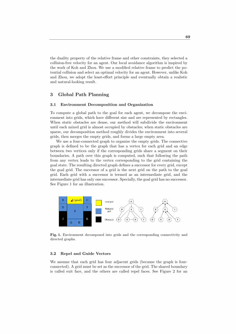
the duality property of the relative frame and other constraints, they selected acollision-free velocity for an agent. Our local avoidance algorithm is inspired bythe work of Koh and Zhou. We use a modified relative frame to predict the po-tential collision and select an optimal velocity for an agent. However, unlike Kohand Zhou, we adopt the least-effort principle and eventually obtain a realisticand natural-looking result.

3 Global Path Planning

3.1 Environment Decomposition and Organization

To compute a global path to the goal for each agent, we decompose the envi-ronment into grids, which have different size and are represented by rectangles.When static obstacles are dense, our method will subdivide the environmentuntil each mixed grid is almost occupied by obstacles; when static obstacles aresparse, our decomposition method roughly divides the environment into severalgrids, then merges the empty grids, and forms a large empty area.

We use a four-connected graph to organize the empty grids. The connectivegraph is defined to be the graph that has a vertex for each grid and an edgebetween two vertices only if the corresponding grids share a segment on theirboundaries. A path over this graph is computed, such that following the pathfrom any vertex leads to the vertex corresponding to the grid containing thegoal state. The resulting directed graph defines a successor for every grid, exceptthe goal grid. The successor of a grid is the next grid on the path to the goalgrid. Each grid with a successor is termed as an intermediate grid, and theintermediate grid has only one successor. Specially, the goal grid has no successor.See Figure 1 for an illustration.

Fig. 1. Environment decomposed into grids and the corresponding connectivity anddirected graphs.

3.2 Repel and Guide Vectors

We assume that each grid has four adjacent grids (because the graph is four-connected). A grid must be set as the successor of the grid. The shared boundaryis called exit face, and the others are called repel faces. See Figure 2 for an

69

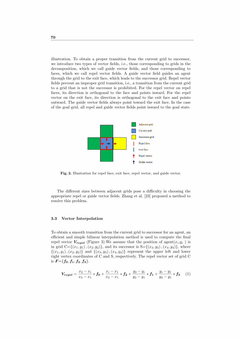
illustration. To obtain a proper transition from the current grid to successor,we introduce two types of vector fields, i.e., those corresponding to grids in thedecomposition, which we call guide vector fields, and those corresponding tofaces, which we call repel vector fields. A guide vector field guides an agentthrough the grid to the exit face, which leads to the successor grid. Repel vectorfields prevent an improper grid transition, i.e., a transition from the current gridto a grid that is not the successor is prohibited. For the repel vector on repelfaces, its direction is orthogonal to the face and points inward. For the repelvector on the exit face, its direction is orthogonal to the exit face and pointsoutward. The guide vector fields always point toward the exit face. In the caseof the goal grid, all repel and guide vector fields point inward to the goal state.

Fig. 2. Illustration for repel face, exit face, repel vector, and guide vector.

The different sizes between adjacent grids pose a difficulty in choosing theappropriate repel or guide vector fields. Zhang et al. [23] proposed a method toresolve this problem.

3.3 Vector Interpolation

To obtain a smooth transition from the current grid to successor for an agent, anefficient and simple bilinear interpolation method is used to compute the finalrepel vector Vrepel (Figure 3).We assume that the position of agent(xi,yi ) isin grid C={(x1, y1) , (x2, y2)}, and its successor is S={(x3, y3) , (x4, y4)}, where{(x1, y1) , (x2, y2)} and {(x3, y3) , (x4, y4)} represent the upper left and lowerright vertex coordinates of C and S, respectively. The repel vector set of grid Cis F={f0,f1,f2,f3}.

Vrepel =x2 − xix2 − x1

∗ f0 +xi − x1x2 − x1

∗ f2 +y2 − yiy2 − y1

∗ f1 +yi − y1y2 − y1

∗ f3 (1)

70

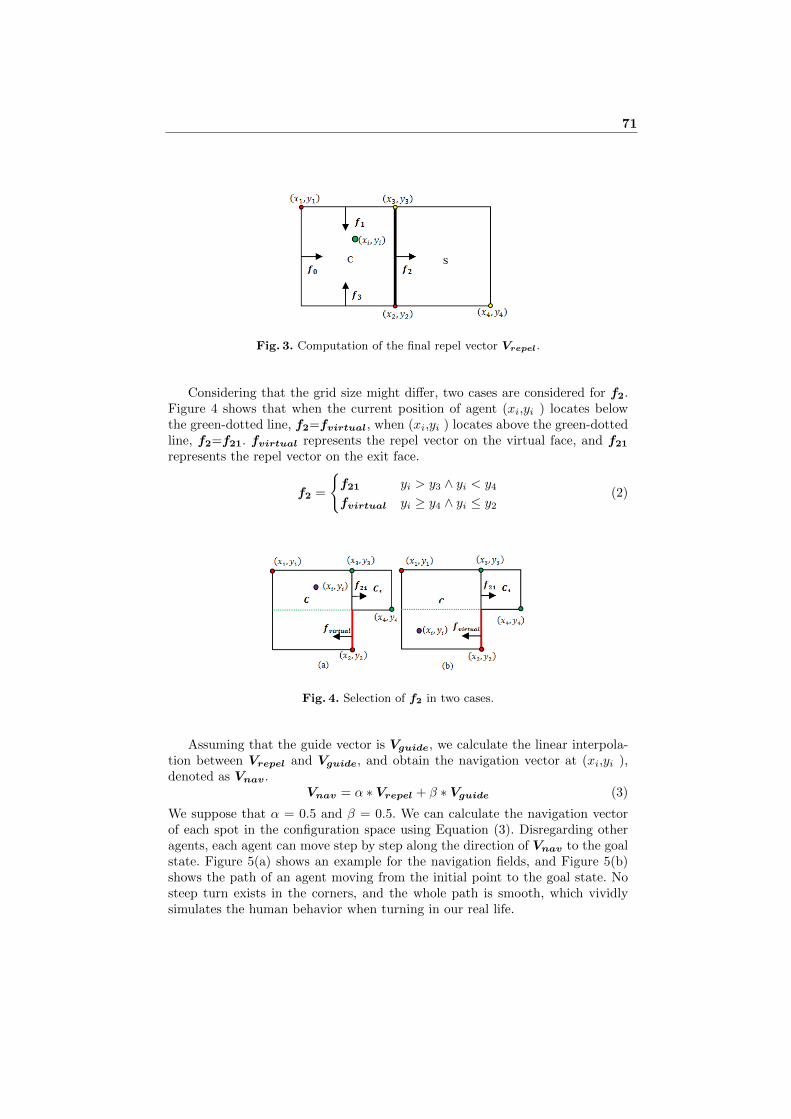
Fig. 3. Computation of the final repel vector Vrepel.

Considering that the grid size might differ, two cases are considered for f2.Figure 4 shows that when the current position of agent (xi,yi ) locates belowthe green-dotted line, f2=fvirtual, when (xi,yi ) locates above the green-dottedline, f2=f21. fvirtual represents the repel vector on the virtual face, and f21

represents the repel vector on the exit face.

f2 =

{f21 yi > y3 ∧ yi < y4

fvirtual yi ≥ y4 ∧ yi ≤ y2(2)

Fig. 4. Selection of f2 in two cases.

Assuming that the guide vector is Vguide, we calculate the linear interpola-tion between Vrepel and Vguide, and obtain the navigation vector at (xi,yi ),denoted as Vnav.

Vnav = α ∗ Vrepel + β ∗ Vguide (3)

We suppose that α = 0.5 and β = 0.5. We can calculate the navigation vectorof each spot in the configuration space using Equation (3). Disregarding otheragents, each agent can move step by step along the direction of Vnav to the goalstate. Figure 5(a) shows an example for the navigation fields, and Figure 5(b)shows the path of an agent moving from the initial point to the goal state. Nosteep turn exists in the corners, and the whole path is smooth, which vividlysimulates the human behavior when turning in our real life.

71

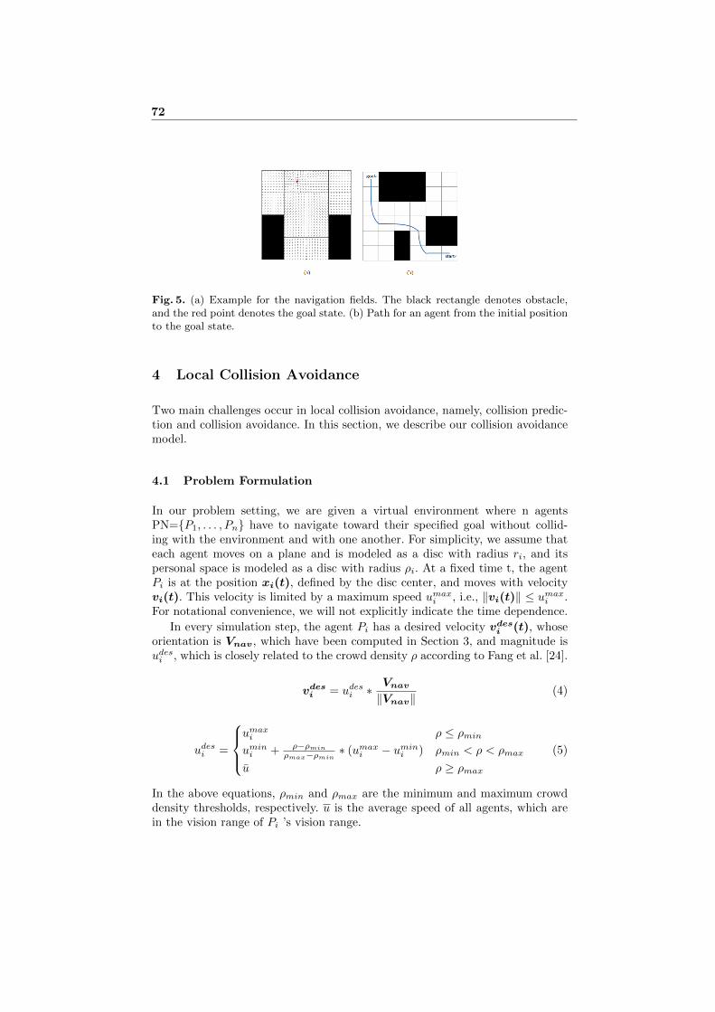
Fig. 5. (a) Example for the navigation fields. The black rectangle denotes obstacle,and the red point denotes the goal state. (b) Path for an agent from the initial positionto the goal state.

4 Local Collision Avoidance

Two main challenges occur in local collision avoidance, namely, collision predic-tion and collision avoidance. In this section, we describe our collision avoidancemodel.

4.1 Problem Formulation

In our problem setting, we are given a virtual environment where n agentsPN={P1, . . . , Pn} have to navigate toward their specified goal without collid-ing with the environment and with one another. For simplicity, we assume thateach agent moves on a plane and is modeled as a disc with radius ri, and itspersonal space is modeled as a disc with radius ρi. At a fixed time t, the agentPi is at the position xi(t), defined by the disc center, and moves with velocityvi(t). This velocity is limited by a maximum speed umaxi , i.e., ‖vi(t)‖ ≤ umaxi .For notational convenience, we will not explicitly indicate the time dependence.

In every simulation step, the agent Pi has a desired velocity vdesi (t), whose

orientation is Vnav, which have been computed in Section 3, and magnitude isudesi , which is closely related to the crowd density ρ according to Fang et al. [24].

vdesi = udesi ∗ Vnav

‖Vnav‖(4)

udesi =

umaxi ρ ≤ ρminumini + ρ−ρmin

ρmax−ρmin∗ (umaxi − umini ) ρmin < ρ < ρmax

u ρ ≥ ρmax(5)

In the above equations, ρmin and ρmax are the minimum and maximum crowddensity thresholds, respectively. u is the average speed of all agents, which arein the vision range of Pi ’s vision range.

72

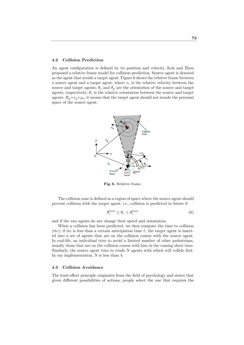
4.2 Collision Prediction

An agent configuration is defined by its position and velocity. Koh and Zhouproposed a relative frame model for collision prediction. Source agent is denotedas the agent that avoids a target agent. Figure 6 shows the relative frame betweena source agent and a target agent, where vr is the relative velocity between thesource and target agents; θs and θg are the orientation of the source and targetagents, respectively; θr is the relative orientation between the source and targetagents. Rg=rg+ρs, it means that the target agent should not invade the personalspace of the source agent.

Fig. 6. Relative frame.

The collision zone is defined as a region of space where the source agent shouldprevent collision with the target agent, i.e., collision is predicted in future if

θminr ≤ θr ≤ θmaxr (6)

and if the two agents do not change their speed and orientation.When a collision has been predicted, we then compute the time to collision

(ttc); if ttc is less than a certain anticipation time t, the target agent is insert-ed into a set of agents that are on the collision course with the source agent.In real-life, an individual tries to avoid a limited number of other pedestrians,usually those that are on the collision course with him in the coming short time.Similarly, the source agent tries to evade N agents with which will collide first.In our implementation, N is less than 4.

4.3 Collision Avoidance

The least-effort principle originates from the field of psychology and states thatgiven different possibilities of actions, people select the one that requires the

73

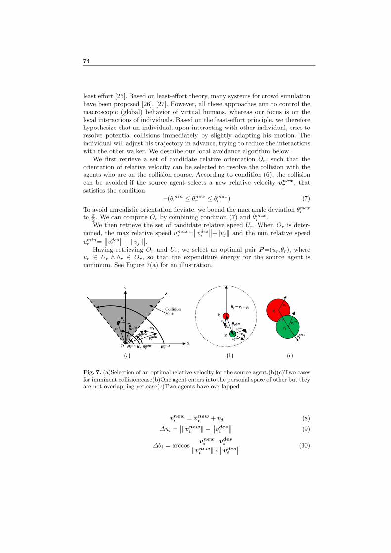
least effort [25]. Based on least-effort theory, many systems for crowd simulationhave been proposed [26], [27]. However, all these approaches aim to control themacroscopic (global) behavior of virtual humans, whereas our focus is on thelocal interactions of individuals. Based on the least-effort principle, we thereforehypothesize that an individual, upon interacting with other individual, tries toresolve potential collisions immediately by slightly adapting his motion. Theindividual will adjust his trajectory in advance, trying to reduce the interactionswith the other walker. We describe our local avoidance algorithm below.

We first retrieve a set of candidate relative orientation Or, such that theorientation of relative velocity can be selected to resolve the collision with theagents who are on the collision course. According to condition (6), the collisioncan be avoided if the source agent selects a new relative velocity vnew

r , thatsatisfies the condition

¬(θminr ≤ θnewr ≤ θmaxr ) (7)

To avoid unrealistic orientation deviate, we bound the max angle deviation θmaxi

to π2 . We can compute Or by combining condition (7) and θmaxi .We then retrieve the set of candidate relative speed Ur. When Or is deter-

mined, the max relative speed umaxr =∥∥vdesi

∥∥+‖vj‖ and the min relative speed

uminr =∣∣∥∥vdesi

∥∥− ‖vj‖∣∣.

Having retrieving Or and Ur, we select an optimal pair P=(ur,θr), whereur ∈ Ur ∧ θr ∈ Or, so that the expenditure energy for the source agent isminimum. See Figure 7(a) for an illustration.

Fig. 7. (a)Selection of an optimal relative velocity for the source agent.(b)(c)Two casesfor imminent collision:case(b)One agent enters into the personal space of other but theyare not overlapping yet.case(c)Two agents have overlapped

vnewi = vnew

r + vj (8)

∆ui =∣∣‖vnew

i ‖ −∥∥vdes

i

∥∥∣∣ (9)

∆θi = arccosvnewi · vdes

i

‖vnewi ‖ ∗

∥∥vdesi

∥∥ (10)

74

In the above equations, ∆ui is the value for speed changed, and ∆i is the angledeviation of the source agent. The cost function is

f(ur, θr) = α ∗ ∆uiumax

+ β ∗ ∆θiθmax

(11)

where umax=1.5m/s is the maximal value for speed changed, and θmax=π2 is the

maximum angle deviation. The constants α and β define the weights of specificcost terms and can vary among the agents to simulate a wide variety of avoidancebehavior.

Computing the minimum value of Equation (11) is time-consuming. Thus,we restrict the domain Or to a discrete set of orientation samples (the defaultsize of the discretization step is set to 0.01π). Similarly, we discretize the domainUr into a set of adjacent speed samples (the default distance between adjacentsamples is set to 0.05). Assuming that the discretized set of Or is Or and thatof Ur is Ur , then the set of admissible relative velocity is

FAVr = {urθr | ur ∈ Ur ∧ θr ∈ Or} (12)

The discretized cost function is

vnewr = argminV cand∈FAVr{

α ∗∣∣∥∥vcand + vj

∥∥−∥∥vdesi

∥∥∣∣umax

+ β ∗ arccos(vcand + vj) · vdesi

‖vcand + vj‖ ∗∥∥vdesi

∥∥

}(13)

Having retrieving vnewr , the optimal new velocity for the source agent is easy tocompute. We then update the source agent position into

xnewi = xi + vnew

i ∗∆t (14)

4.4 Resolve Imminent Collision

We divide imminent collision into two cases (Figure 7(b)(c)). In case (b), weintroduce the concept of relative tangential velocity, which is equivalent to ap-plying a tangential force to separate the two agents. In case (c), we introducethe concept of repel velocity, which is equivalent to applying a repulsive force toseparate the two agents immediately.

4.5 Avoiding Static Obstacles

An agent Ai also needs to avoid colliding with the static obstacles of the envi-ronment. In our simulations, such obstacles are modeled as axis aligned boxes.Collisions are resolved by following an approach similar to the one describedabove.

We first retrieve the nearest obstacles of the agent Ai that are inside the visualfield of the agent. We then compute the maximum and minimum orientationsamong the vectors lined from the current position of Ai ’s to each vertex of theconvex polygon obstacle. The maximum and minimum orientations are θmaxr andθminr , respectively, which have been discussed above. Finally, we use a least-effortcriterion to select an optimal velocity for the agent Ai.

75

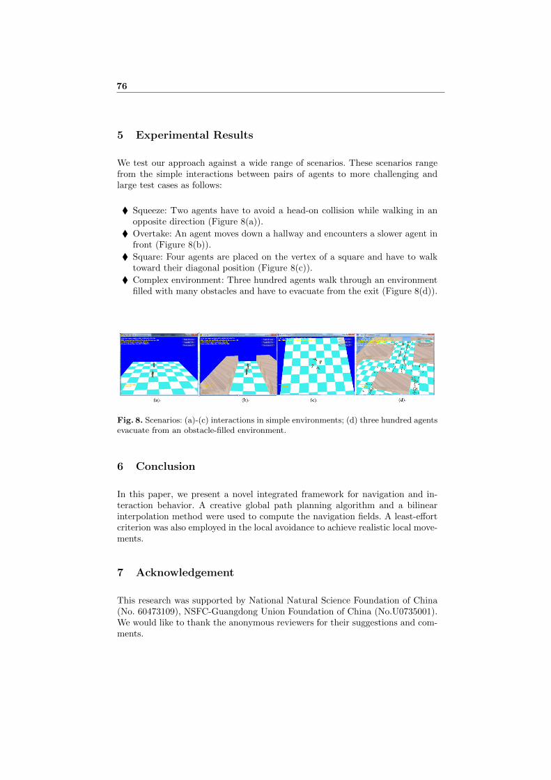
5 Experimental Results

We test our approach against a wide range of scenarios. These scenarios rangefrom the simple interactions between pairs of agents to more challenging andlarge test cases as follows:

� Squeeze: Two agents have to avoid a head-on collision while walking in anopposite direction (Figure 8(a)).

� Overtake: An agent moves down a hallway and encounters a slower agent infront (Figure 8(b)).

� Square: Four agents are placed on the vertex of a square and have to walktoward their diagonal position (Figure 8(c)).

� Complex environment: Three hundred agents walk through an environmentfilled with many obstacles and have to evacuate from the exit (Figure 8(d)).

Fig. 8. Scenarios: (a)-(c) interactions in simple environments; (d) three hundred agentsevacuate from an obstacle-filled environment.

6 Conclusion

In this paper, we present a novel integrated framework for navigation and in-teraction behavior. A creative global path planning algorithm and a bilinearinterpolation method were used to compute the navigation fields. A least-effortcriterion was also employed in the local avoidance to achieve realistic local move-ments.

7 Acknowledgement

This research was supported by National Natural Science Foundation of China(No. 60473109), NSFC-Guangdong Union Foundation of China (No.U0735001).We would like to thank the anonymous reviewers for their suggestions and com-ments.

76

References

1. Treuille A, Cooper S, Popovi? Z. Continuum crowds[C]. ACM Transactions onGraphics (TOG). ACM, 2006, 25(3): 1160-1168.

2. Helbing D, Molnar P. Social force model for pedestrian dynamics[J]. Physical re-view E, 1995, 51(5): 4282-4286.)

3. Shao W, Terzopoulos D. Autonomous pedestrians[C]. Proceedings of the 2005 ACMSIGGRAPH/Eurographics, 2005: 19-28.

4. Hao Jiang, et al., A Semantic Environment Model for Crowd Simulation in Mul-tilayered Complex Environment. VRST 2009, Kyoto, Japan, November 18 C 20,2009. pp191-198

5. Kraayenbrink N, Kessing J, Tutenel T, et al. Semantic crowds. EntertainmentComputing[J], 2014(5):297-312

6. Paris S, Donikian S, Bonvalet N. Environmental abstraction and path planningtechniques for realistic crowd simulation[J]. Computer Animation and VirtualWorlds, 2006, 17(3-4): 325-335.

7. Pettre J, Laumond J P, Thalmann D. A navigation graph for real-time crowdanimation on multilayered and uneven terrain[C]. First International Workshop onCrowd Simulation. 2005, 43(44): 194-202.

8. Bandi S, Thalmann D. Space discretization for efficient human navigation[C]. Com-puter Graphics Forum. Blackwell Publishers Ltd, 1998, 17(3): 195-206.

9. Bayazit O B, Lien J M, Amato N M. Better Group Behaviors in Complex Envi-ronments using Global Roadmaps[J]. Artificial Life 8, 2003: 362-371.

10. Sud A, Andersen E, Curtis S, et al. Real-time path planning in dynamic virtualenvironments using multiagent navigation graphs[J]. Visualization and ComputerGraphics, IEEE Transactions on, 2008, 14(3): 526-538.

11. Philippsen R, Siegwart R. An interpolated dynamic navigation function[C].Robotics and Automation, 2005. ICRA 2005. Proceedings of the 2005 IEEE Inter-national Conference on. IEEE, 2005: 3782-3789.

12. Dapper F, Prestes E, Idiart M A P, et al. Simulating pedestrian behavior withpotential fields[M]. Advances in Computer Graphics. Springer Berlin Heidelberg,2006: 324-335.

13. Lindemann S R, LaValle S M. Simple and efficient algorithms for computing s-mooth, collision-free feedback laws over given cell decompositions[J]. The Interna-tional Journal of Robotics Research, 2009, 28(5): 600-621.

14. Park M J. Guiding flows for controlling crowds[J]. The Visual Computer, 2010,26(11): 1383-1391.

15. Patil S, Van Den Berg J, Curtis S, et al. Directing crowd simulations using naviga-tion fields[J]. Visualization and Computer Graphics, IEEE Transactions on, 2011,17(2): 244-254.

16. Karamouzas I, Heil P, van Beek P, et al. A predictive collision avoidance modelfor pedestrian simulation[M]. Motion in Games. Springer Berlin Heidelberg, 2009:41-52.

17. Van den Berg J, Lin M, Manocha D. Reciprocal velocity obstacles for real-timemulti-agent navigation[C]. Robotics and Automation, 2008. ICRA 2008. IEEE In-ternational Conference on. IEEE, 2008: 1928-1935.

18. Ondrej J, Pettr J, Olivier A H, et al. A synthetic-vision based steering approach forcrowd simulation[J]. ACM Transactions on Graphics (TOG), 2010, 29(4): 123-131.

19. Paris S, Pettr J, Donikian S. Pedestrian reactive navigation for crowd simulation:a predictive approach[C]. Computer Graphics Forum. Blackwell Publishing Ltd,2007, 26(3): 665-674.

77

20. Karamouzas I, Overmars M. Simulating human collision avoidance using a velocity-based approach[C]. Workshop in Virtual Reality Interactions and Physical Simu-lation. The Eurographics Association, 2010: 125-134.

21. Karamouzas I, Overmars M. Simulating and evaluating the local behavior of smallpedestrian groups[J]. Visualization and Computer Graphics, IEEE Transactionson, 2012, 18(3): 394-406.

22. Wee Lit Koh and SuiPing Zhou. Modeling and Simulation of Pedestrian Behaviorin Crowded Places. ACM Transactions on Modeling and Computer Simulation,2011, 21(3): 20-42.

23. Zhang L, LaValle S M, Manocha D. Global vector field computation for feedbackmotion planning[C]. Robotics and Automation, 2009. ICRA’09. IEEE InternationalConference on. IEEE, 2009: 477-482.

24. Fang Z, Lo S M, Lu J A. On the relationship between crowd density and movementvelocity[J]. Fire Safety Journal, 2003, 38(3): 271-283.

25. George K. Zipf. Human behavior and the principle of least effort[J]. Addison-Wesley, 1949. 3.

26. Safonova A, Hodgins J K. Construction and optimal search of interpolated motiongraphs[C]. ACM Transactions on Graphics (TOG). ACM, 2007, 26(3): 106-116.

27. Guy S J, Curtis S, Lin M C, et al. Least-effort trajectories lead to emergent crowdbehaviors[J]. Physical Review E, 2012, 85(1): 016110.

78

Position on Interoperability Everywhere underIoT-ARM

Adriano Tavares1, Fausto Giunchiglia2, Hao Xu3, and Yanchun Liang3

1DEI, University of Minho, 4800058, Portugal2DISI, University of Trento, 38100, Italy

3CCST, Jilin University, Changchun, 130012, Chinaatavares@dei.uminho.pt

fausto@disi.unitn.it

{xuhao,ycliang}@jlu.edu.cn

Abstract. This position paper argues that accelerating the use of IoT-ARM (Architectural Reference Model) on new IoT-Systems’ realizationsrequires semantic interoperability to more than architectural, device andconnectivity levels but also at tool-, system stack-, language- and work-flow management-level. In doing so, an IoT-ARM ontology is proposedwhich extends the conceptual model of IoT-ARM method with highly co-hesive Methodology Mapping, Big Data Analytic, and Architecture Im-plementation Roadmap facets while leveraging cross- and intra-languageinteroperability.

Keywords: Semantic Interoperability, Multi-Lingual Interoperability,Big Data, Open Data, IoT, Ontology, IoT-ARM.

1 Introduction

Currently, we are entering the Internet of Things (IoT)-age with IoT-systemsconsisting of components like sensing, heterogeneous access, information process-ing and, applications and services. IoT movement relies on pervasive connectivityand intelligently connects humans, devices, and systems by integrating multipletechnologies under a unified management platform. Architecturally, IoT followsa serviced-oriented model and it can be split into four tiers. Thing-tier for sensingand transmission, Intelligent System-tier (i.e., Fog-tier) for early-life data analy-sis, aggregation and transmission, Cloud-tier for early-life or at-rest science-dataanalysis and storing and, Application-tier for user access and control.

Driven by the heterogeneity of IoT-related ecosystems, several problem spaceshave been identified like connectivity, architecting process, big data analytics,device intelligence and data technologies that must be overcome to achieve main-stream IoT adoption. As IoT spans various industries and use cases, embed-ded processing will demand scalable strategies while a limited scope of stan-dards will coexist for a long time to come as one size will not fit all [1, 2].IoT-ARM emerged as a possible answer to the IoT multiplicity issue and it

started by creating the IoT Reference Model (IoT-RM) to promote a com-mon understanding, followed by the IoT Reference Architecture (IoT-RA) thatdescribes essential building blocks and design choices to deal with conflictingquality attributes like functionality, performance, deployment and security [3,4]. IoT-ARM approaches a loosely-coupled interoperability at connectivity- andsemantic-level and it relies on the semantic technology to apply interoperabil-ity at architectural-level through the IoT Domain Model and IoT InformationModel. It also addresses connectivity interoperability using a service-orientedcommunication model leveraged on the ISO OSI 7-layer model and it aims athighlighting those peculiar interoperability aspects inherent to the interoperationamong different stacks, which are called interoperability features. Furthermore,it builds variation points into the software, and uses standard extension points,e.g., using standardized protocols and gateways to enable brownfield deployment[3].

From our point of view, IoT-ARM presents some drawbacks that are decel-erating its use on new IoT-Systems’ realizations such as:

• It only partially addresses device technology issues as its focus is only on thesoftware stack (i.e., it does not address the whole system stack).

• Its Architecting Process is too generic and so, several projects instead offollowing IoT-ARM from the ground up try to show at the end of theirarchitecture realizations how do they map to the IoT-ARM (e.g., [5]).

• It does not explicitly promote the interplay of IoT with Big Data as itsmain focus goes to IoT applications for track, command, control and route(TCC&R) purposes.

2 Our Approach

Our approach aims at designing a modular ontology to assist in IoT-ARM Ar-chitecting Process (i.e., IoT-ARM ontology) as an instance of UKC [6, 7]. TheUKC domain, concept, and entity type cores will be extended by terminologyspecific to a new field of study, in order to assist semantically the IoT-ARMArchitecting Process which is denominated IoT-ARM ontology. Basically, IoT-ARM ontology is a synthesis of ontologies proposed in [8, 9], extended with theMethodology Mapping facet to accommodate IoT-ARM methodology agnosti-cism and Big Data Analytic facet to enable interplay of IoT with Big Data.Extending IoT-ARM with the idea of Everywhere Interoperability based on ascalable semantic schema built as an instance of UKC will leverage:

• Multi-Lingual Interoperability at both cross-language and intra-languagelevels. Cross-language interoperability among several languages will enabletheir entrance into the ”Open Big Data Age” while intra-language interoper-ability allows the use of multiple terms denoting the same concepts or morespecific/general terms.

• Declarative design of a semantic and scalable whole design stackfor easy customization at each IoT tier and better addressing the increasing

80

intelligence, security, safety, communication, timeliness, area, and power is-sues. The Architectural Description facet is extended with specific sub-facetsrepresenting the required knowledge for co-design strategies and propagationeffects among the stack layers while the Architecture Design facet with atechnological design flow sub-facet for the whole stack design. All entitiesincluding tools (e.g., design, simulation, synthesis tools) are declarativelyand semantically tagged for the purpose.

• Semantic collaborative system design chain according to known work-flow reference model dictated by industry horizontalization. The Architec-ture Implementation Roadmap facet is extended with a business collabora-tion workflow sub-facet embedding industry chain management knowledge.

• Big Data Analytic Reference Architecture to model Big Data Ana-lytics space problem in terms of several levels of heterogeneity involved onits architecting and design process, at analytical types, use cases scenarios,location of analytic technology, analytic techniques, type of actionable intel-ligence and visualization, sources and type of data, technological platforms,spectrum of analytical workloads, etc.

To support the proposed multi-level interoperability, we are using SCROLLNLP and UKC frameworks developed by the KnowDive team at University ofTrento. Following the UKC’s so-called faceted approach to ontological model-ing, the IoT-ARM ontology is extended by a large number of concepts (e.g., Sw,Hw and Simulation components, views, tactics, design choice, perspectives, qual-ity attributes, system, design stack, design flow), entities (e.g., Linux, Windows,FreeRTOS, OSGi framework, ARM Cortex-M3, MPSoC, Hadoop, Oracle, Open-Stack, VMWare, Cassandra, Simulink, Modelica), and highly cohesive facets(e.g., Methodology Mapping, Architectural Description, Architectural Require-ments, Architecture Design, Architecture Implementation Roadmap). SCROLLNLP has been extended to support several languages by collecting linguisticresources, adapting and integrating them into a processing pipeline.

Following standardization on ontology leverages abilities of a gradually grow-ing IoT-ARM environments (i.e., by skipping out of the ”Standard War”), map-ping of different vendors/providers technologies to the IoT-ARM, tooling en-ablement from different vendors/providers to the IoT-ARM environment andready-made ecosystem of partners, thus enabling IoT-Systems’ realizations ofseveral and different use cases scenarios. After populating IoT-ARM ontologywith several catalogs of entities divided by categories and semantically taggedwith their properties and constraints, tools for managing templates of systemstack and development flow through functionalities such as creation, instantia-tion, configuration, validation and deployment are designed and implemented. Ateam of experts in a given IoT application domain can create templates for spe-cific applications and use cases scenarios (i.e., enabling some kind of applicationguidance) and populate the associated catalogs after validation. Furthermore,they specify mapping strategies described as semantics rules to associate tacticsto design choices and then add them to the IoT-ARM tactic and design choicecatalog. Later a user can instantiate existing template seeds from the catalog

81

for his/her new IoT system realization. If a template contains abstract compo-nents/tools, then the component/tool catalog is queried to find a valid bind.

Several reasoners will be implemented to: (1) reason about the design space,(2) assist in the creation of design flows and system stacks, (3) reason about com-ponents’ constraints and tool’s characteristics and propagate them through thedevelopment flow and system stack structures and (4) reason about the matchingbetween a development flow and a system stack. After reasoning about the designspace and identifying all valid instances of system stack, a virtual prototypingenvironment can be built to explore such solution space. Such environment is aspecialization or specific instance of the development flow to carry out mixed-simulation, including the dynamics of the physical process using tools such asSimulink or Modelica which are possible entities of IoT-ARM ontology populatedinto the catalog of tools. According to the IoT-ARM architectural description, areasoner will be provided for each qualitative requirement to find a perspectiveassociated with it and also to select tactics based on the functional requirementsand architectural constraints. Finally, semantics rules are proposed to prioritizethe way that perspectives will be applied to views as not all perspectives haveequal effect on all views.

3 Opportunities Addressed

By extending IoT-ARM ontology to be more focused on main IoT current issuesfaced by new IoT-related system realizations, such as, technical, architecture,hardware, privacy and security, standard and business challenges, the conceptualmodel of IoT-ARM method is improved by tackling its poor methodologicalcompleteness and application guidance as pointed in [10] while promoting:

• Multi-sourced and multi-lingual big data analytics supporting real-time opendata.

• Interoperability at stakeholder-level while mitigating IoT market fragmen-tation and industry disjointed tooling ecosystem.

• 3C (Computing, Control and Communication)- and 3S (Scalability, Securityand Safety)-convergences in the new ’Cloud + Edge’ computing paradigmthrough a holistic collaborative design chain approach encompassing end-device, connectivity layer, gateway, and services running in the cloud withdesign metrics or quality attributes factored in at every level.

• Some level of automation and application guidance to the IoT-ARM ar-chitecting process by approaching semantic whole system stack as well assemantic design flow with interoperability at tool-level.

Acknowledgments. The authors would like to acknowledge the assistance ofDrs. Gabor Bella, Feroz Farazi and Enzo Maltese at the University of Trento,and PhD students Sandro Pinto and Paulo Garcia at the University of Minho,for their useful discussions and efforts on writing related proposals. The firstauthor is grateful to the support of FCT - Fundacao para a Ciencia e Tecnologia

82

in the scope of the project: PEst-UID/CEC/00319/2013. The last two authorsare grateful to the support of the NSFC (61272207, 61300147, 61472158).

References

1. Karimi, K., Atkinson, G.: What the Internet of Things (IoT) Needs to Become aReality. In: Freescale White Paper (2013)

2. Xing, Z.H., Zhong, Y.F.: Internet of Things and its future. In: Huawei Communicate,Issue 54 (2010)

3. Bassi, A., Bauer, M., Fiedler, M., Kramp, T., Kranenburg, R., Lange, S., Meissner,S.: Enabling Things to Talk: Designing IoT solutions with the IoT ArchitecturalReference Model. ISBN 978-3-642-40403-0, Springer (2013)

4. Kim, Y.-W.: IoT Reference Architecture versus IoT Platform From StandardizationViewpoint, http://docbox.etsi.org/Workshop/2014/201407_IOTWORKSHOP/ETRI_KIM.pdf (2014)

5. Kiljander, J., D’Elia, A., Morandi, F., Hyttinen, P., Takalo-Mattila, J., Ylisaukko-Oja, A., Soininen, J.-P., Cinotti, T.S.: Semantic Interoperability Architecture forPervasive Computing and Internet of Things. In: IEEE Open Access Journal, Vol-ume 2 (2014)

6. Tawfik, A., Giunchiglia, F., Maltese, V.: A Collaborative Platform for MultilingualOntology Development. Technical Report, Trento University (2014)

7. Ganbold, A., Farazi, F., Giunchiglia, F.: Managing Language Diversity across Cul-tures: the English-Mongolian Case Study. Technical Report, Trento University(2013)

8. Akerman, A., Tyree, J.: Using Ontology to Support Development of Software Ar-chitectures. In: IBM Systems Journal (45:4), pp. 813-825 (2006)

9. Ameller, D., Franch, X.: Ontology-Based Architectural Knowledge Representation:Structural Elements Module. In: Advanced Information Systems Engineering Work-shops, Lecture Notes in Business Information Processing, Springer Berlin Heidel-berg, pp. 296-301 (2011)

10. Nikitina, S.: Translating Qualitative Requirements into Design Choices: Evalu-ating the Method Proposed in the Architectural Reference Model for the Inter-net of Things. Master thesis, http://iotforum.org/wp-content/uploads/2014/

10/Nikitina_S_Thesis.pdf (2014)

83

A Proposal of a Model using Kansei Evaluationintegrated with Fuzzy Rules and Self-Organizing

Map for Evaluation of Bio-Food Products

Hai Van Pham? and Khang Dinh Tran

School of Information Technology and Communication, Hanoi University of Scienceand Technology

No.1, Dai Co Viet St., Hanoi, Vietnam

{haipv,khangtd}@soict.hust.edu.vn

Abstract. Agricultural product intelligence is a new way for biotech-nology that can be made multiple food products with a variety of char-acteristics, enhanced flavor and nutritional quality of foods. To evaluatefood products of bio-food products for improvement of the food qualityin global bio-food markets, cross-cultural customer behaviors are mostlyinfluenced with healthy food in global markets. In this study, we proposea new approach using Kansei Evaluation integrated with fuzzy rules andSelf-Organizing Map (SOM) model, together with customers and expertsensibilities and preferences for selection of the appropriate alternatives(bio-food and food technology), matched with mass customer and ex-pert group behaviors. To confirm the model’s performance, the proposedapproach has been tested in experiments for the validated model andapplied in several domains in Asian countries.

Keywords: Kansei Evaluation, Food Biotechnology, Bio-food Evalua-tion, fuzzy rules, Self-Organizing Maps

1 Introduction

The potential food biotechnology is a key biotechnology engineering to pro-duce good bio-food, attractive marketing, or healthy nutrition in daily life. Foodbiotechnology has been widely produced healthy foods in daily life [1]. Foodbiotechnology is one of the ways quickly producing fresh foods and improvingquality. Researchers need to determine if each potential new food product willbe a useful, beneficial and safe development. Customers and consumers wouldbe expected good food products as well as quality foods. In conventional meth-ods [1] [2] [5] [6], most approaches have been investigated bio-food evaluation ofgood features based on food factory standards. However, the weaken points of

? Corresponding to Hai Van Pham, email: haipv@soict.hust.edu.vn

these approaches using group customer/expert sensibilities and preferences arenot aggregated concurrently that affects to evaluate a bio-food quality in termsof customer feedbacks. In food biology evaluation, Kansei evaluation makes itpossible to quantify expert and customer perception, sensation, cognition, sen-timent, and impression about food quality [3]. In Kansei Evaluation, we havedetermined adjective pairs called Kansei words in pairs: Synonym - Antonym,Synonym - Not Synonym. For instance, the pairs of adjectives ”good - bad”and”satisfied- not satisfied”are Kansei words. Emotions are part of human behaviorin certain sensibilities that affect human final decisions [3]. Collaborative Deci-sion Making (CDM) can be defined as a decision problem with the selection ofalternatives, using CDM obtains dynamic decision solutions talking into accountthese preferences. Self-Organizing Maps (SOMs) were invented by Kohonen asa computational method for the visualization of high-dimensional data [4]. Thestudy in this paper is to solve the existing problems in a dynamic evaluationof the appropriate alternatives (bio-food, food technology and food product) indynamic markets. The aim of proposed approach is to evaluate alternatives (bio-food, food technology and food products), using Collaborative Decision Making(CDM), together with expert sensibilities and emotions. The advantages of theproposed approach are presented in this paper by dealing with multi-culturalcustomers in market dynamics as follows: 1) qualitative factors with uncertaintyin dynamic market conditions, consisting of expert preferences are consideredthrough the model; 2) the framework is used to quantify expert’s sensibilities andemotions using collaborative decision making decisions. To confirm the model’sperformance, the proposed system has been validated by experimental resultsfor the demonstration of this study.

2 Kansei Evaluation in quantification of human sensibilityand behavior

2.1 Kansei word matrix construction

In the preliminary experiment, the surveys were done by 30 customers includinglocal, international students and experts from Hanoi Fresh Vegetable and FruitInstitute with export companies for the markets. There were 5 experts and 25customers who participated in the surveys for selection of 14 adjectives as pairsof Kansei words in total of 16 Kansei words influenced to these criteria. In thefinal data collection, we have selected 14 Kansei words of the most relevant wordswith redundance of 02 Kansei words using Factor Analysis that are influencedto these criteria for evaluation of biology-food products, as shown in Table 1.

A Kansei matrix is constructed using Kansei words for the steps as follows:

1. Collect customer surveys in the preliminary experiment using Semantic Dif-ferential (SD) method with a five-point scale definition (0: oppose, 0.25:almost oppose, 0.5: have no preference, 0.75: almost agree, 1: agree).

2. Consider the most appropriate Kansei words in the bio-food market belong-ing to Kansei criteria evaluation.

86

3. Structure Kansei words using Factor Analysis to identify conditional factorloadings and commonalities in the model.

4. Select the most appropriate Kansei words and construct a Kansei matrixfrom the average of Kansei weights.

5. Update Kansei weights to the Kansei matrix in a Database.

Table 1. Pairs of Kansei words for Kansei evaluation

No Positive word Negative word Factor Criteria Evaluation

1 Good Not good Product name2 Pleasant Unpleasant Bio-food product3 Famous Not famous Brand name Product Information4 Flavor Not flavor Customer satisfactory5 Cheap Expensive Bio-food Price

6 Satisfactory Not satisfactory Product quality7 Low High Customer satisfactory8 Acceptable Not acceptable International standard Product9 Satisfactory Unsatisfactory Customer behavior quality

10 Global Local International market11 Stable Changing Asian market Markets12 Standing Falling Government market

13 Liked Disliked Asian culture Culture14 Preferable Not preferable Vietnamese culture

2.2 Kansei matrix evaluation

Let XS = {XS1 , X

S2 , ..., X

Sm} be a set of Kansei words that use to evaluate bio-

food products, where m is the number of Kansei words. In order to quantifycustomer’s sensibilities in evaluating bio-food products, we have refined for themost important Kansei words in XS to evaluate a bio-food product with respectto criteria in stock market S.

Let WSm = {W−m ,W+

m} be opposite pairs of Kansei words with respect toXS

m. Let P customers collect their preferences by surveys. To evaluate bio-foodproduct CS

j , its Kansei weight wtij represents by the i-th Kansei word of the

j-th bio-food product evaluated by the t-th expert. Hence, the average weight ofi-th Kansei word is evaluated by P customers, as given by Eq.(1).

kSij =1

P

P∑

t=1

wtij (1)

87

KSn×m = (kSij)(n×m) is a Kansei matrix construction, where n and m is the

number of bio-food products and Kansei words respectively. Table 2 illustratesa sample of the Kansei matrix consisting of alternatives in Kansei evaluation.

Table 2. The Kansei score matrix in an evaluation

ID No XS1 XS

2 ... XS16 Bio-food product

1 k11 k12 ... k1m P1

... ... ... ... ... ...

n kn1 kn2 ... knm Pn

3 Proposed approach

3.1 Human emotions in decision making

Human emotions in decision making can be presented as an integration of log-ical rules, quantitative knowledge and reasoning evidence. Figure 1 shows thequantification of expert sensibilities and emotions.

In common sense human reasoning, linguistic expressions represent rules forexpert decision situations. To quantify emotions and sensibilities in reasoning ofexpert in dynamic market environments, we use fuzzy rules as illustrations of anexample as follows:Rule 1: IF Japanese people prefer an organic apple juice with its red color ANDsatisfaction with its fresh fruit THEN The system marks positive emotion statusliked++Rule 2: IF Chinese people do not like an organic apple juice AND Chinesemarkets have many fresh apples with these low prices THEN The system marksnegative emotion status disliked- -Note that emotion expert status represents in the subset disliked- -, disliked-,neutral, satisfied+, satisfied++, as described human reasoning emotion deci-sions.

Common Sense Human Reasoning can be presented as an integration of fuzzyrules, quantitative knowledge and reasoning evidence. Linguistic expressions canbe used to represent rules for expert decision situations. To quantify the CommonSense Human Reasoning of expert ei in dynamic market environments, we usethe following logical rules as Rule i can be expressed by Eq.(1):

IF Condition 1 AND...AND Condition m

THEN Actions

Note that expert decision status is represented in a five step scale {invest++,invest+, neutral, risk-, risk- -}

88

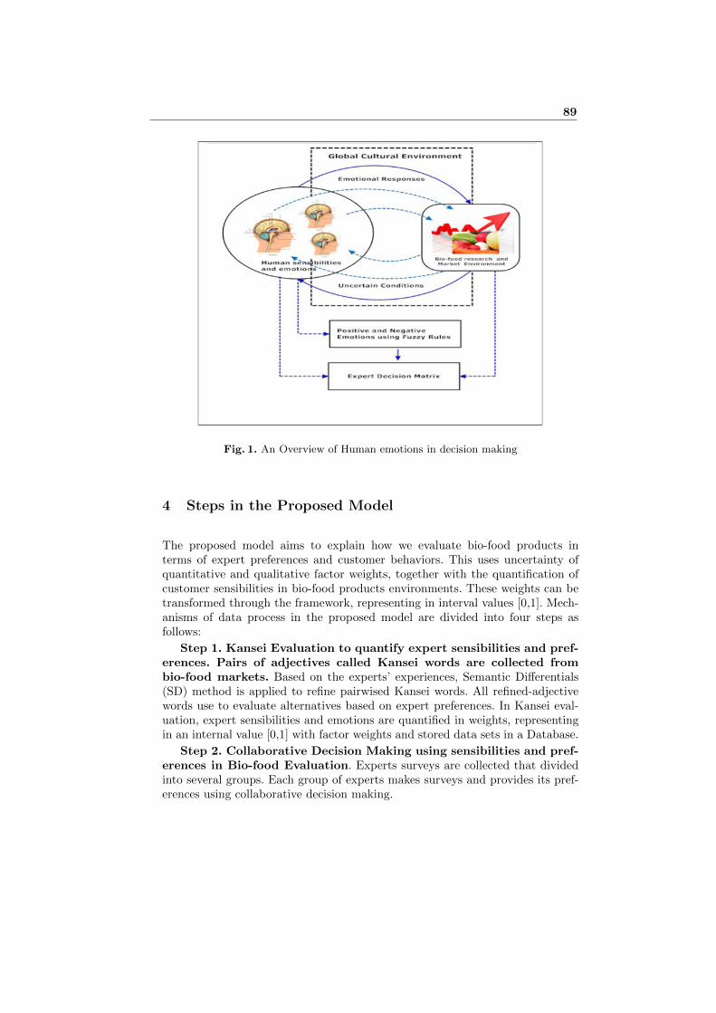
Fig. 1. An Overview of Human emotions in decision making

4 Steps in the Proposed Model

The proposed model aims to explain how we evaluate bio-food products interms of expert preferences and customer behaviors. This uses uncertainty ofquantitative and qualitative factor weights, together with the quantification ofcustomer sensibilities in bio-food products environments. These weights can betransformed through the framework, representing in interval values [0,1]. Mech-anisms of data process in the proposed model are divided into four steps asfollows:

Step 1. Kansei Evaluation to quantify expert sensibilities and pref-erences. Pairs of adjectives called Kansei words are collected frombio-food markets. Based on the experts’ experiences, Semantic Differentials(SD) method is applied to refine pairwised Kansei words. All refined-adjectivewords use to evaluate alternatives based on expert preferences. In Kansei eval-uation, expert sensibilities and emotions are quantified in weights, representingin an internal value [0,1] with factor weights and stored data sets in a Database.

Step 2. Collaborative Decision Making using sensibilities and pref-erences in Bio-food Evaluation. Experts surveys are collected that dividedinto several groups. Each group of experts makes surveys and provides its pref-erences using collaborative decision making.

89

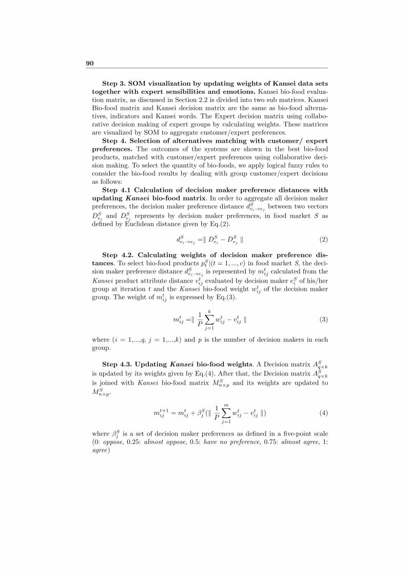
Step 3. SOM visualization by updating weights of Kansei data setstogether with expert sensibilities and emotions. Kansei bio-food evalua-tion matrix, as discussed in Section 2.2 is divided into two sub matrices. KanseiBio-food matrix and Kansei decision matrix are the same as bio-food alterna-tives, indicators and Kansei words. The Expert decision matrix using collabo-rative decision making of expert groups by calculating weights. These matricesare visualized by SOM to aggregate customer/expert preferences.

Step 4. Selection of alternatives matching with customer/ expertpreferences. The outcomes of the systems are shown in the best bio-foodproducts, matched with customer/expert preferences using collaborative deci-sion making. To select the quantity of bio-foods, we apply logical fuzzy rules toconsider the bio-food results by dealing with group customer/expert decisionsas follows:

Step 4.1 Calculation of decision maker preference distances withupdating Kansei bio-food matrix. In order to aggregate all decision makerpreferences, the decision maker preference distance dSei→ej between two vectors

DSei and DS

ej represents by decision maker preferences, in food market S asdefined by Euclidean distance given by Eq.(2).

dSei→ej =‖ DSei −DS

ej ‖ (2)

Step 4.2. Calculating weights of decision maker preference dis-tances. To select bio-food products pSt |(t = 1, ..., c) in food market S, the deci-sion maker preference distance dSei→ej is represented by mt

ij calculated from the

Kansei product attribute distance vtij evaluated by decision maker eSi of his/hergroup at iteration t and the Kansei bio-food weight wt

ij of the decision makergroup. The weight of mt

ij is expressed by Eq.(3).

mtij =‖ 1

P

k∑

j=1

wtij − vtij ‖ (3)

where (i = 1,...,q, j = 1,...,k) and p is the number of decision makers in eachgroup.

Step 4.3. Updating Kansei bio-food weights. A Decision matrix ASq×k

is updated by its weights given by Eq.(4). After that, the Decision matrix ASq×k

is joined with Kansei bio-food matrix MSn×p and its weights are updated to

MSn×p.

mt+1ij = mt

ij + βSj (‖ 1

P

m∑

j=1

wtij − vtij ‖) (4)

where βSj is a set of decision maker preferences as defined in a five-point scale

(0: oppose, 0.25: almost oppose, 0.5: have no preference, 0.75: almost agree, 1:agree)

90

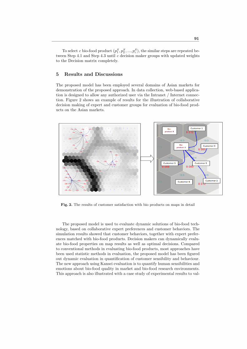
To select c bio-food product (pS1 , pS2 , ..., p

Sc ), the similar steps are repeated be-

tween Step 4.1 and Step 4.3 until c decision maker groups with updated weightsto the Decision matrix completely.

5 Results and Discussions

The proposed model has been employed several domains of Asian markets fordemonstration of the proposed approach. In data collection, web-based applica-tion is designed to allow any authorized user via the Intranet / Internet connec-tion. Figure 2 shows an example of results for the illustration of collaborativedecision making of expert and customer groups for evaluation of bio-food prod-ucts on the Asian markets.

Fig. 2. The results of customer satisfaction with bio products on maps in detail

The proposed model is used to evaluate dynamic solutions of bio-food tech-nology, based on collaborative expert preferences and customer behaviors. Thesimulation results showed that customer behaviors, together with expert prefer-ences matched with bio-food products. Decision makers can dynamically evalu-ate bio-food properties on map results as well as optimal decisions. Comparedto conventional methods in evaluating bio-food products, most approaches havebeen used statistic methods in evaluation, the proposed model has been figuredout dynamic evaluation in quantification of customer sensibility and behaviour.The new approach using Kansei evaluation is to quantify human sensibilities andemotions about bio-food quality in market and bio-food research environments.This approach is also illustrated with a case study of experimental results to val-

91

idate the model. In future works, the proposed approach is extended to evaluatemultiple food products in daily life.

6 Conclusion

The proposed approach has been applied in evaluation of bio-food products,based on collaborative expert preferences and customer behaviors. The simula-tion results showed that customer behaviors, together with expert preferencesmatched with bio-food products. Decision makers can dynamically evaluate bio-food properties on map results as well as optimal decisions. The new approachusing Kansei evaluation is to quantify expert sensibilities and emotions aboutbio-food quality in market and bio-food research environments. This approach isalso illustrated with a case study of experimental results to validate the model.In future works, the proposed approach is extended to evaluate multiple foodproducts in daily life.

References

1. Nolwennig R., Jean R., and Gard D, 2009, Information effects on consumer attitudestoward three food technologies: Organic production, biotechnology, and irradiation,Food Quality and Preference (20) 586-596.

2. Rita Batista, Maria Margarida Oliveira, 2009, Facts and fiction of genetically engi-neered food, Trends in Biotechnology (27) 277-286.

3. Salem, B. and Nakatsu, R. and Rauterberg, M., 2005, Kansei Experience: Aesthetic,Emotions and Inner Balance, International Journal of Cognitive Informatics andNatural Intelligence (3) 54-64.

4. T. Kohonen,(1995), Sefl-Organizing Maps, Spiringer-verlag.5. Bologna, and Italy, 2013, Bio-based technologies in the context of European Food

Innovation Systems: Outcomes from the EFFoST Annual Meeting, Trends in FoodScience and Technology, (37) 162-165

6. P.M. Davidson, H. Bozkurt Cekmer, E.A. Monu, C. Techathuvanan, 2015, The useof natural antimicrobials in food: An overview, Handbook of Natural Antimicrobialsfor Food Safety and Quality, (5) 1-27

92

Improved algorithm of unsatisfiability-based MaximumSatisfiability

Yiyuan Wang, Dantong Ouyang, Liming Zhang∗

Symbol Computation and Knowledge Engineering of Ministry of Education, Jilin University,Changchun 130012, China

College of Computer Science and Technology, Jilin University, Changchun 130012, China

Abstract. Recently, the Maximum Satisfiability (MaxSAT) discovers a rapid-ly increasing number of practical applications in a wide range of different ar-eas. Unsatisfiability-based MaxSAT algorithms have been put forward aimed atimproving the performance of solving MaxSAT problem. In these algorithms,several excellent Boolean Satisfiability (SAT) solvers are employed to iterative-ly identify unsatisfiable sub-formulas and the additional blocking variables arealso applied to relax some of initial clauses or encode Boolean constraints intoa CNF formula. Firstly, this paper proposes two novel optimizations to reducethe search space: finding all disjoint unsatisfiable cores with the original clausesremoved and no blocking variables added; avoiding generating the largest num-ber of blocking variables’ clauses with heuristic strategy. Moreover, in order toreduce the number of satisfying iterations, the partial assignment is introducedinto satisfiability-based framework as the tight bound accelerator which couldfind a smaller number of blocking variables. Experimental results show that theunsatisfiability-based algorithm with these optimizations results in an improvedand more effective solver for MaxSAT problem than previous algorithms. In ad-dition,this results in consistent performance gains in most cases and on average1.5 times speed-up for MaxSAT with state-of-the-art algorithms.

Introduction

The classical NP-complete problem of Boolean Satisfiability (SAT) [8] has been agrowth of interest in not just the theoretical computer science community, but also invarious areas where feasible solutions to these problems are significantly important inmany practical applications. These practical applications have been able to successfullyapply SAT as a decision procedure to determine whether these instances are SAT orUNSAT. However, there are more extra demands of the SAT problem that exceed thisdecision procedure of SAT solvers, such as Maximum Satisfiability problem (MaxSAT)[12, 3] and Pseudo-Boolean Optimization (PBO). Moreover, using the strong relation-ship between these problems, several new algorithms have been developed [21].

MaxSAT as a well-known problem in Computer Science, consists of identifying thelargest number of clauses in a CNF formula that can be satisfied. The recent applica-tion of MaxSAT and variants in design debugging and verification of complex designs[4, 10, 20] motivated the development of new MaxSAT algorithms, capable of solving

large structured problem instances common to these application domains. Many exac-t methods for finding MaxSAT have been developed in recent years. Davis-Putnam-Logemann-Loveland procedure [5] explores a binary search tree and then establishesincrementally truth assignments. The result of several methods based on this procedureis very good, but they are not suitable for MaxSAT practical problems. Some other ex-act methods generally based on Branch and Bound (B&B) algorithms [2] have beendesigned to handle MaxSAT, but are unable to solve majority of problem instances.Recently algorithms based on the identification of unsatisfiable sub-formulas [7, 18, 19,15], with blocking variables introduced into these algorithms and Pseudo Boolean Op-timization used to simplify CNF, have also been developed, and are now able to tackleall these Boolean optimization problems and most of unsatisfiable instances.

This paper firstly reviews previous MaxSAT algorithm based on unsatisfiable sub-formulas named msu4 [19], and then proposes an improved MaxSAT algorithm basedon the method of binary search [11]. Despite the improved algorithm building on msu4based on unsatisfiable sub-formulas and binary search, this paper proposes one im-provement as the tight bound accelerator and extra two optimizations to reduce thesearch space, which are novel, including: (1) reducing the number of SAT solver iter-ations under the control of partial assignment; (2) developing the heuristic strategy toavoid generating the largest number of blocking clauses, so as to slow down the effi-ciency of algorithm, when the middle value is half number of blocking variables. (3)speeding up to find all disjoint unsatisfiable cores without blocking variables added in-to these clauses in the early iterative execution of binary search’s preprocess. The newimproved algorithm also uses several techniques [6] to utilize BDDs for encoding cardi-nality constraints as Boolean circuits. Experimental results show that the new MaxSATalgorithm is observably faster than the previous MaxSAT algorithms in a wide rangeof unsatisfiable industrial instances, demonstrating the robustness of the proposed ap-proach.

Preliminaries

Firstly a finite set of Boolean variables is assumed X={x1,x2,x3,. . . ,xn}. A CNF for-mula φ is defined on the conjunction of clauses wi and each clause consists of thedisjunction of literals, which is either a variable xi or its complement xi. In the con-text of search algorithms of SAT, variables can be assigned a logic value, either 0 or 1.Alternatively, variables can defined as a function v: X →{0,u,1}, where u denotes avariable whose value is uncertain. When all of variables are assigned a value in {0,1},then v is referred to as a complete assignment. Otherwise it is a partial assignment [17]where some variables do not have values and are assigned u, which will be used in thefollowing improved algorithm.

In this section Maximal Satisfiability and Minimal Unsatisfiability are firstly intro-duced. Afterwards, the previous MaxSAT algorithm using unsatisfiable cores namedmsu4 is described.

94

Maximal Satisfiability and Minimal Unsatisfiability

Our improved algorithm and previous methods are based on maximal satisfiability andminimal unsatisfiability. The MaxSAT problem as an optimization problem correspondsto the minimization of the number of false clauses in a CNF formula, which meansthat MaxSAT problem discovers an assignment to the variables of a CNF formula thatmaximizes the number of satisfied clauses.

In order to illustrate this problem, Maximally Satisfiable Subset (MSS) is defined asa subset of clauses in a CNF formula, which is satisfiable and then adds any of the otherclauses in an original formula to MSS leading new clauses set to unsatisfiable. In thiscontext, Minimal Unsatisfiable Subset (MUS) is an inconsistent subset of the clauses ofthe original formula and dropping one of its clauses will make it satisfiable. MSS andMUS [14, 7] correspond to the following rules:

MSS(φ) =

{m is satisfiable, if m⊆φ

m ∪ {a} is unsatisfiable, ∀a∈(φ-m)

MUS(φ) =

{m is unsatisfiable, if m⊆φ

m − {a} is satisfiable, ∀a∈m

Notice that MSS as a satisfied subset of clauses cannot become bigger and MUS asan unsatisfiable subset that removes any of its clauses can render it satisfiable. The rela-tionship between MaxSAT and MSS is subtle. Given an unsatisfiable instance, MaxSATis the largest subset of clauses that can be satisfiable which means to find MSS withmaximal number. However, all MSSes may have different sizes and cannot be al-l MaxSAT solutions with maximal number. Removing the clauses that are not includedin the MSS makes CNF formula satisfiable. Therefore Minimal Correction Set (MCS)is introduced to describe the complement of MSS and the set of MCSes is shown:

MCSes(φ) = {m|m ⊆ φ and (φ − m) ∈ MSSes(φ)}

MCS as the complementary point of MSSes offers the real link to MUSes. Notethat any clause of MUS in a CNF formula makes the formula unsatisfiable and thecomplement formula satisfiable,thus every MSS must contain at least one of clauses ofevery MUS. This relationship between MCSes and MUSes can usually be described asa solution to a set converting problem. Specifically, each hitting set of the MUSes isan MCS. Given a collection of sets, hitting set intersects all sets in the collection in atleast one element and the problem of hitting set is an equivalent reformulation of setcovering. A MCS is a hitting set of the MUSes with the additional limit that it cannotbecome smaller without losing its defining property: it is an irreducible hitting set andeach hitting set of MCSes is an MUS. The example formula is shown to explain theirrelationship between MSSes, MCSes and MUSes.

φ = (x1) ∧ (x1 ∨ x2) ∧ (x2) ∧ (x2)

MSSes(φ) ={{x1, x1 ∨ x2, x2}, {x1 ∨ x2, x2}, {x1, x2}

}

95

MCSes(φ) ={{x2}, {x1, x2}, {x1 ∨ x2, x2}

}

MUSes(φ) ={{x1, x1 ∨ x2, x2}, {x2, x2}

}

In the example above, every MUS of a CNF formula is an irreducible hitting setof the MCSes of that CNF formula. In the given CNF formula above, the number ofmaximal satisfiable clauses is 3. More importantly, MSS and MUS also can tell us therelationship between MUS and MaxSAT problem.

A MaxSAT algorithm using unsatisfiable cores

Recently, several methods based on unsatisfiable cores are proposed. Msu4 which ap-plies improved blocking variable into clauses is more effective than other algorithms inthe experiment results. More importantly, msu4 avoids interacting with a PBO solverand instead is a fully SAT-based solver that relies on the most effective techniques,such as Boolean Constraint Propagation, conflict based learning and conflict-directedbacktracking [16]. Finally, the two advantages of msu4 lie in adding at most one block-ing variable into each clause in a CNF formula which can avoid quickly increasing thenumber of blocking variables and clauses, and applying linear programming encodingof pseudo boolean constraints with BDDs and sorting networks.

Proposition 1 MaxSAT Upper Bound(UB): In a CNF formula, φ corresponds to thenumber of clauses. Let K denote disjoint unsatisfiable cores, then φ-K corresponds toan MaxSAT Upper Bound.

Proposition 2 MaxSAT Lower Bound(LB): Let B define as the set of blocking vari-ables assigned value TRUE when clauses become satisfiable, then φ-B denotes a MaxSATLower Bound.

In previous subsection, some relationships between MUS and MaxSAT are brieflyintroduced and these properties are employed in the algorithm to define MaxSAT UpperBound and Lower Bound [19]. Some details for msu4 are shown in [19].

Improved MaxSAT algorithm with some strategies

As shown previously, unsatisfiable-based algorithm is able to tackle MaxSAT problem.However, msu4 works by the redundant lower and upper bounds in some SAT solveriterations. This section proposes an improved algorithm based on msu4 with two keyoptimizations, which are used as the tight bound accelerator. Firstly the thought of bi-nary search [11] (its algorithm named BIN ) can be imported into msu4 for clearlyimproving its efficiency by decreasing the redundant calculation. Secondly, based onthe idea of binary search, this paper proposes some key optimizations: (1)the use ofpartial assignment computing a smaller number of blocking variables assigned value

96

TRUE instead of the middle value of binary search in each satisfying assignment. (2)theheuristic strategy HSBS to avoid generating the largest number of clauses containingblocking variables when the middle value is nearly half number of blocking variables.(3)acceleration to find disjoint unsatisfiable cores by iteratively computing the originalformula and temporarily deleting these cores that have already been found.

Unsatisfiable core-based MaxSAT algorithm using binary search

In algorithm 1, compared with the upper bound and lower bound in the msu4, two newbounds, which denote the lower and upper bounds of lower bound, are firstly proposedand then used into algorithm 1 and algorithm 2.

Proposition 3 Lower Bound of Lower Bound (L LB): φ corresponds to a CNF for-mula. Remove any L LB clauses to render new φ∗ unsatisfiable. In our algorithm 2,L LB is initialized to the number of unsatisfiable cores.

Proposition 4 Upper Bound of Lower Bound (L UB):φ corresponds to a CNF formu-la. Remove the given L UB clauses to make new φ∗ satisfiable. In algorithm 2, L UBis firstly assigned to the number of blocking variables.

Proposition 5 [11] Binary search for MaxSAT executes Θ(log(W )) calls to a SAToracle in the worst case.

Compared with msu4, algorithm 1 uses the method of binary search to acquireMaxSAT solution and is also based on Proposition 5 defined in the BIN to guidealgorithm 1. The pseudo code for msu5 bin is shown in Algorithm 1.

In msu4, lower bound only depends on the value of blocking variables when φis satisfiable, and its variation is passive. Considering that msu4 calculates the sizeof lower bound by inches, this paper presents the binary search, whose algorithm incomputer science finds the position of a specified value within a sorted key. Algorithm 1employs the binary search to take the initiative to alter two bounds in order to acceleratethe growth of two bounds for reducing the number of SAT solver iterations, which willsolve the MaxSAT problem quickly.

In algorithm 1, there are several differences between msu4 and msu5 bin. L UB isinitialized to the number of initial clauses and L LB is to 0. Before each call to the SATsolver, BSB which corresponds to the middle variable, needs to be computed under themethod of binary search (line 6). Afterwards CNF (

∑i∈VB

bi ≤ BSB) is generatedand then added to φw (line 7 and 8). L LB is only updated on iterations when theSAT solver returns false. Considering such an iteration, for which the unsatisfiable coredoes not include initial clauses (line 17), L LB will be assigned to BSB . When theunsatisfiable core contains original clauses I > 0, this process is the same as msu4from line 13 to 16. Consider now a satisfiable iteration. It occurs when the numberof blocking variables assigned 1 is sufficient to make the current CNF formula get asatisfiable assignment, L UB will be updated(line 21). But it can not guarantee thatthis number is minimal. When L LB + 1 ≥ L UB, it is an answer of the MaxSATsolution.

97

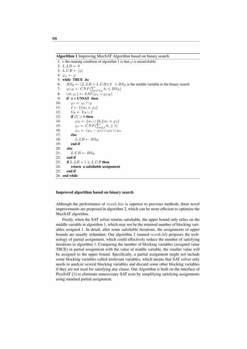
Algorithm 1 Improving MaxSAT Algorithm based on binary search1: ◃ the running condition of algorithm 1 is that φ is unsatisfiable2: L LB ← 03: L UB ← |φ|4: φw ← φ5: while TRUE do6: BSB ← (L LB + L UB)/2 ◃ BSB is the middle variable in the binary search7: φCH ← CNF (

∑i∈VB

bi ≤ BSB)

8: (st, φc)← SAT (φw ∪ φCH)9: if st = UNSAT then

10: φI ← φc ∩ φ11: I ← {i|wi ∈ φI}12: VB ← VB ∪ I13: if |I| > 0 then14: φN ← {wi ∪ {bi}|wi ∈ φI}15: φa ← CNF (

∑i∈I

bi ≥ 1)16: φw ← (φw − φI) ∪ φN ∪ φa

17: else18: L LB ← BSB

19: end if20: else21: L UB ← BSB

22: end if23: if L LB + 1 ≥ L UB then24: return a satisfiable assignment25: end if26: end while

Improved algorithm based on binary search

Although the performance of msu5 bin is superior to previous methods, three novelimprovements are proposed in algorithm 2, which can be more efficient to optimize theMaxSAT algorithm.

Firstly, when the SAT solver returns satisfiable, the upper bound only relies on themiddle variable in algorithm 1, which may not be the minimal number of blocking vari-ables assigned 1. In detail, after some satisfiable iterations, the assignments of upperbounds are usually redundant. Our algorithm 2 (named msu6 bd) proposes the tech-nology of partial assignment, which could effectively reduce the number of satisfyingiterations in algorithm 1. Comparing the number of blocking variables (assigned valueTRUE) in partial assignment with the value of middle variable, the smaller value willbe assigned to the upper bound. Specifically, a partial assignment might not includesome blocking variables called irrelevant variables, which means that SAT solver onlyneeds to analyze several blocking variables and discard some other blocking variablesif they are not used for satisfying any clause. Our Algorithm is built on the interface ofPicoSAT [1] to eliminate unnecessary SAT tests by simplifying satisfying assignmentsusing standard partial assignment.

98

Algorithm 2 Our Improved MaxSAT Algorithm based on binary search1: ◃ the running condition of algorithm 2 is that φ is unsatisfiable2: INC ← ϕ; UNC ← ϕ; CSC ← ϕ; VB ← ϕ3: while st = SAT do4: (st, φc)← increSAT (φ− INC)5: if st = UNSAT then6: VB ← VB ∪ {i|wi ∈ φc}7: INC ← INC ∪ φc

8: UNC ← UNC ∪ {wi ∪ {bi}|wi ∈ φc}9: CSC ← CSC ∪ CNF (

∑i∈φc

bi ≥ 1)10: end if11: end while12: φw ← (φ− INC) ∪ UNC ∪ CSC

13: L LB ← |INC |; L UB ← |VB |14: while TRUE do15: BSB ← (HSBS(L LB))?(L LB + L UB)/2 : (3L LB + L UB)/4 ◃ heuristic

strategy reduces the size of CNF formula16: φCH ← CNF (

∑i∈VB

bi ≤ BSB)

17: (st, φc)← increSAT (φw ∪ φCH)18: if st = UNSAT then19: φI ← φc ∩ φ20: I ← {i|wi ∈ φI}21: VB ← VB ∪ I22: if |I| > 0 then23: φN ← {wi ∪ {bi}|wi ∈ φI}24: φa ← CNF (

∑i∈I

bi ≥ 1)25: φw ← (φw − φI) ∪ φN ∪ φa

26: else27: L LB ← BSB

28: end if29: else30: VS←|the number of blocking variables assigned value 1|31: L UB ← (VS < BSB)?VS : BSB ◃SAT solver selects partial assignment32: end if33: if L LB + 1 ≥ L UB then34: return a satisfiable assignment35: end if36: end while

Secondly, when the middle variable in algorithm 1 is assigned to half number ofblocking variables, it could generate the largest number of clauses for pseudo booleanconstraints. Considering that x1 + x2 + . . . + xn ≥ k results in BDDs with (n −k + 1) × k nodes [6], the number of BDD nodes is maximum when k = n/2. Basedon above, algorithm 2 proposes the heuristic strategy HSBS to avoid this situation inbinary search. The heuristic HSBS function is, when BSB is approximately equal to|VB |/2, BSB is assigned to (3L LB + L UB)/4 which is nearly equal to |VB |/4.

99

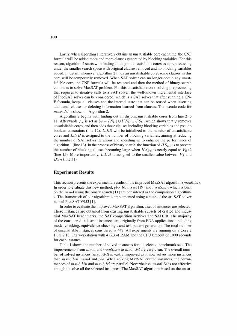
Lastly, when algorithm 1 iteratively obtains an unsatisfiable core each time, the CNFformula will be added more and more clauses generated by blocking variables. For thisreason, algorithm 2 starts with finding all disjoint unsatisfiable cores as a prepossessingunder the smaller search space with original clauses removed and no blocking variablesadded. In detail, whenever algorithm 2 finds an unsatisfiable core, some clauses in thiscore will be temporarily removed. When SAT solver can no longer obtain any unsat-isfiable core, the CNF formula will be restored and then the method of binary searchcontinues to solve MaxSAT problem. For this unsatisfiable core-solving preprocessingthat requires to iterative calls to a SAT solver, the well-known incremental interfaceof PicoSAT solver can be considered, which is a SAT solver that after running a CN-F formula, keeps all clauses and the internal state that can be reused when insertingadditional clauses or deleting information learned from clauses. The pseudo code formsu6 bd is shown in Algorithm 2.

Algorithm 2 begins with finding out all disjoint unsatisfiable cores from line 2 to11. Afterwards φw is set as (φ − INC) ∪ UNC ∪ CSC , which shows that φ removesunsatisfiable cores, and then adds those clauses including blocking variables and pseudoboolean constraints (line 12). L LB will be initialized to the number of unsatisfiablecores and L UB is assigned to the number of blocking variables, aiming at reducingthe number of SAT solver iterations and speeding up to enhance the performance ofalgorithm 1 (line 13). In the process of binary search, the function of HSBS is to preventthe number of blocking clauses becoming large when HSBS is nearly equal to VB/2(line 15). More importantly, L UB is assigned to the smaller value between VS andBSB (line 31).

Experiment Results

This section presents the experimental results of the improved MaxSAT algorithm (msu6 bd).In order to evaluate this new method, pbo [6], msu4 [19] and msu5 bin which is builton the msu4 using the binary search [11] are considered as the comparison algorithm-s. The framework of our algorithm is implemented using a state-of-the-art SAT solvernamed PicoSAT-V953 [1].

In order to evaluate the improved MaxSAT algorithm, a set of instances are selected.These instances are obtained from existing unsatisfiable subsets of crafted and indus-trial MaxSAT benchmarks, the SAT competition archives and SATLIB. The majorityof the considered industrial instances are originally from EDA applications, includingmodel checking, equivalence checking , and test pattern generation. The total numberof unsatisfiable instances considered is 447. All experiments are running on a Core 2Dual 2.13 Ghz workstation with 4 GB of RAM and the CPU timeout of 1000 secondsfor each instance.

Table 1 shows the number of solved instances for all selected benchmark sets. Theimprovements from msu4 and msu5 bin to msu6 bd are very clear. The overall num-ber of solved instances (msu6 bd) is vastly improved as it now solves more instancesthan msu5 bin, msu4 and pbo. When solving MaxSAT crafted instances, the perfor-mances of msu5 bin and msu6 bd are parallel. Nevertheless, msu6 bd is not effectiveenough to solve all the selected instances. The MaxSAT algorithm based on the unsat-

100

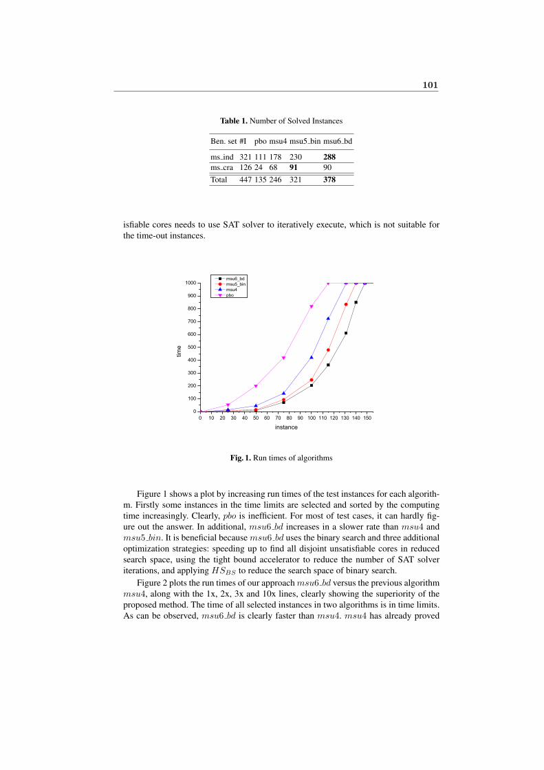
Table 1. Number of Solved Instances

Ben. set #I pbo msu4 msu5 bin msu6 bd

ms ind 321 111 178 230 288ms cra 126 24 68 91 90Total 447 135 246 321 378

isfiable cores needs to use SAT solver to iteratively execute, which is not suitable forthe time-out instances.

0 10 20 30 40 50 60 70 80 90 100 110 120 130 140 1500

100

200

300

400

500

600

700

800

900

1000

time

instance

msu6_bd msu5_bin msu4 pbo

Fig. 1. Run times of algorithms

Figure 1 shows a plot by increasing run times of the test instances for each algorith-m. Firstly some instances in the time limits are selected and sorted by the computingtime increasingly. Clearly, pbo is inefficient. For most of test cases, it can hardly fig-ure out the answer. In additional, msu6 bd increases in a slower rate than msu4 andmsu5 bin. It is beneficial because msu6 bd uses the binary search and three additionaloptimization strategies: speeding up to find all disjoint unsatisfiable cores in reducedsearch space, using the tight bound accelerator to reduce the number of SAT solveriterations, and applying HSBS to reduce the search space of binary search.

Figure 2 plots the run times of our approach msu6 bd versus the previous algorithmmsu4, along with the 1x, 2x, 3x and 10x lines, clearly showing the superiority of theproposed method. The time of all selected instances in two algorithms is in time limits.As can be observed, msu6 bd is clearly faster than msu4. msu4 has already proved

101

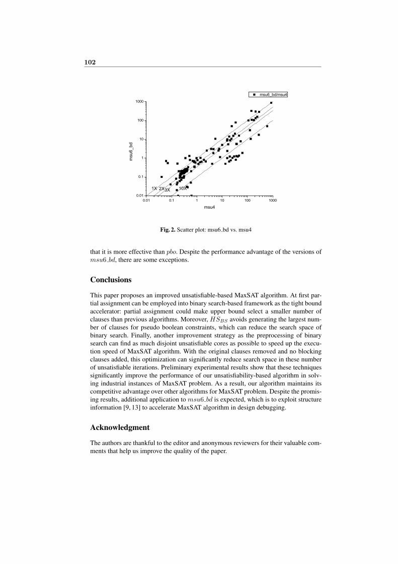
0.01 0.1 1 10 100 10000.01

0.1

1

10

100

1000

msu6_bd/msu4

msu6_bd

msu4

1X 2X3X 10X

Fig. 2. Scatter plot: msu6 bd vs. msu4

that it is more effective than pbo. Despite the performance advantage of the versions ofmsu6 bd, there are some exceptions.

Conclusions

This paper proposes an improved unsatisfiable-based MaxSAT algorithm. At first par-tial assignment can be employed into binary search-based framework as the tight boundaccelerator: partial assignment could make upper bound select a smaller number ofclauses than previous algorithms. Moreover, HSBS avoids generating the largest num-ber of clauses for pseudo boolean constraints, which can reduce the search space ofbinary search. Finally, another improvement strategy as the preprocessing of binarysearch can find as much disjoint unsatisfiable cores as possible to speed up the execu-tion speed of MaxSAT algorithm. With the original clauses removed and no blockingclauses added, this optimization can significantly reduce search space in these numberof unsatisfiable iterations. Preliminary experimental results show that these techniquessignificantly improve the performance of our unsatisfiability-based algorithm in solv-ing industrial instances of MaxSAT problem. As a result, our algorithm maintains itscompetitive advantage over other algorithms for MaxSAT problem. Despite the promis-ing results, additional application to msu6 bd is expected, which is to exploit structureinformation [9, 13] to accelerate MaxSAT algorithm in design debugging.

Acknowledgment

The authors are thankful to the editor and anonymous reviewers for their valuable com-ments that help us improve the quality of the paper.

102

References1. Biere, A.: Picosat essentials. Journal on Satisfiability, Boolean Modeling and Computation

4(75-97), 45 (2008)2. Borchers, B., Furman, J.: A two-phase exact algorithm for max-sat and weighted max-sat

problems. Journal of Combinatorial Optimization 2(4), 299–306 (1998)3. Cai, S., Luo, C., Thornton, J., Su, K.: Tailoring local search for partial maxsat. In: Twenty-

Eighth AAAI Conference on Artificial Intelligence (2014)4. Chen, Y., Safarpour, S., Marques-Silva, J., Veneris, A.: Automated design debugging with

maximum satisfiability. Computer-Aided Design of Integrated Circuits and Systems, IEEETransactions on 29(11), 1804–1817 (2010)

5. Davis, M., Logemann, G., Loveland, D.: A machine program for theorem-proving. Commu-nications of the ACM 5(7), 394–397 (1962)

6. Een, N., Sorensson, N.: Translating pseudo-boolean constraints into sat. Journal on Satisfia-bility, Boolean Modeling and Computation 2(3-4), 1–25 (2006)

7. Fu, Z., Malik, S.: On solving the partial max-sat problem. Theory and Applications of Satis-fiability Testing-SAT 2006 pp. 252–265 (2006)

8. Gary, M., Johnson, D.: Computers and Intractability: A Guide to the Theory of NP-completeness. WH Freeman and Company, New York (1979)

9. Guo, T., Li, Z., Guo, R., Zhu, X.: Large scale diagnosis using associations between sys-tem outputs and components. In: Twenty-Fifth AAAI Conference on Artificial Intelligence(2011)

10. Heras, F., Larrosa, J., Oliveras, A.: Minimaxsat: A new weighted max-sat solver. Theory andApplications of Satisfiability Testing–SAT 2007 pp. 41–55 (2007)

11. Heras, F., Morgado, A., Marques-Silva, J.: Core-guided binary search algorithms for max-imum satisfiability. In: Proceedings of the AAAI National Conference (AAAI). pp. 36–41(2011)

12. Johnson, D.: Approximation algorithms for combinatorial problems. Journal of computerand system sciences 9(3), 256–278 (1974)

13. Le, B., Mangassarian, H., Keng, B., Veneris, A.: Non-solution implications using reversedomination in a modern sat-based debugging environment. In: Design, Automation & Testin Europe Conference & Exhibition (DATE), 2012. pp. 629–634 (2012)

14. Liffiton, M., Sakallah, K.: On finding all minimally unsatisfiable subformulas. In: Theoryand Applications of Satisfiability Testing. pp. 34–42 (2005)

15. Manquinho, V., Martins, R., Lynce, I.: Improving unsatisfiability-based algorithms forboolean optimization. Theory and Applications of Satisfiability Testing–SAT 2010 pp. 181–193 (2010)

16. Manquinho, V., Marques-Silva, J.: Search pruning techniques in sat-based branch-and-boundalgorithms for the binate covering problem. Computer-Aided Design of Integrated Circuitsand Systems, IEEE Transactions on 21(5), 505–516 (2002)

17. Marques-Silva, J., Lynce, I., Malik, S.: Conflict-driven clause learning sat solvers. SATHandbook pp. 131–154 (2009)

18. Marques-Silva, J., Planes, J.: On using unsatisfiability for solving maximum satisfiability.arXiv preprint arXiv:0712.1097 (2007)

19. Marques-Silva, J., Planes, J.: Algorithms for maximum satisfiability using unsatisfiablecores. In: Proceedings of the conference on Design, automation and test in Europe. pp. 408–413 (2008)

20. Zhang, L., Bacchus, F.: Maxsat heuristics for cost optimal planning. In: Proceedings of theAAAI National Conference (AAAI) (2012)

21. Zhu, Z., Li, C., Manya, F., Argelich, J.: A new encoding from minsat into maxsat. In: Prin-ciples and Practice of Constraint Programming. pp. 455–463 (2012)

103

Entailment-based Axiom Pinpointingin Debugging Incoherent Terminologies

Yuxin Ye1,2, Dantong Ouyang1,2? , Jing Su2

1 College of Computer Science and Technology, Jilin University,Changchun 130012, China

2 Key Laboratory of Symbolic Computation and Knowledge Engineering of Ministryof Education, Changchun 130012, China

{yeyx,ouyd}@jlu.edu.cn

sujing11@mails.jlu.edu.cn

Abstract. One of the major problems of axiom pinpointing for incoher-ent terminologies is the precise positioning within the conflict axioms. Inthis paper we present a formal notion for the entailment-based axiompinpointing of incoherent terminologies, where the parts of an axiom isdefined by atomic entailment. Based on these concepts, we prove theone-to-many relationship between existing axiom pinpointing with theentailment-based axiom pinpointing. For its core task, calculating min-imal unsatisfiable entailment, we provide algorithms for OWL DL ter-minologies using incremental strategy and Hitting Set Tree algorithm.The feasibility of our method is shown by case study and experimentevaluations.

Keywords: ontology debugging, description logics, pinpointing, MUPS

1 Introduction

Ontology debugging becomes a challenging task for ontology modelers since theimprovement of expressivity of ontology language and ontology scale[1]. Axiompinpointing [2] is an important mean for ontology debugging. Any approachwhich can detect a set of axioms in the terminology that lead to logic conflict isbelong to axiom pinpointing. It can be categorized into MSSs (maximally satisfi-able sub-TBox), MUPS (minimal unsatisfiable sub-TBox) and justification. Forfinding maximally concept-satisfiable terminologies, Meyer[3] proposes a tableaulike procedure for terminologies represented in ALC. The approach of Meyer isextended by Lam[4] to get a fine-grained axiom pinpointing for ALC terminolo-gies. In addition, several methods have been proposed to calculate the MUPS.Schlobach and Cornet[5] provide complete algorithms for unfoldable ALC-TBoxbased on minimization of axioms for MUPS, then Schlobach[6, 7] presents aframework for the debugging of logically contradicting terminologies. Parsia[8]

? Corresponding author: Dantong Ouyang, Email: ouyd@jlu.edu.cn

extends Schlobach[5] to more expressive DLs. Baader[2] presents automata-basedalgorithms for reasoning in DLs with the pinpointing formula whose minimal val-uations correspond to the MUPS. From the perspective of unsatisfiability, jus-tification is the MUPS of an unsatisfiable concept. Kalyanpur has explored thedependencies between unsatisfiable classes[9], and proposed several approachesfor computing all justifications of an entailment in an OWL-DL ontology[10]. De-bugging tasks in OWL ontologies are in general computationally hard, so someoptimization techniques are introduced for ontology debugging such as heuristicmethod[11] of identifying common errors and inferences, and modularization[12]for large ontologies. On the whole, various approaches achieve the result setsof axioms responsible for an unsatisfiable concept or a incoherent terminology.Hasse[13] provides a set of criteria for comparing between different approachesrelated to ontology debugging directly or indirectly, and that none of the sur-veyed approaches is universally applicable for any application scenario. Axiompinpointing identifies conflict axioms, but practical problems remain. It is notclear which parts of axioms lead to the conflicts. and some contradictions wouldbe lost[14]. In this paper, we try to give other notion of axiom pinpointing forincoherent terminologies, and define algorithms for this task.

The rest of this paper is organized as follows. In section 2 we briefly introducethe drawback of MUPS. Then the formal definitions about fine-grained axiompinpointing, and the link with axiom pinpointing are presented in section 3.Section 4 presents algorithm for calculating the minimal unsatisfiable entailment.Section 5 analyzes the fine-grained axiom pinpointing with a case study andevaluates the algorithm by experimenting with common ontologies. Finally, weconclude the paper in section 6.

2 Drawback of MUPS

Axiom pinpointing[2] has been introduced in description logics to help the us-er to understand the reasons why consequences hold and to remove unwantedconsequences by computing minimal subsets of the terminology that have theconsequence. The axiom pinpointing we discuss in this paper is MUPS[5]. It’suseful for relating sets of axioms to the unsatisfiability of specific concept.

Definition 1 (MUPS[5]). A TBox T ′ ⊆ T is a minimal unsatisfiability p-reserving sub-TBox (MUPS) for C in T if C is unsatisfiable in T ′, and C issatisfiable in every sub-TBox T ′′ ⊂ T ′. The set of all MUPS of C in T is de-noted as mups(T , C).

Most existing approaches can obtain the different fine-grained problematicaxioms on the basis of axiom pinpointing as none of these approaches defineexactly what they mean by parts of axioms. Further, some logic contradictionswould be lost with axiom pinpointing since it does not point out the specificlocation within the axioms of the logic contradiction. Let us use an example toillustrate these limitations.

106

Example 1. A TBox T1 consists of the following axioms (α1−α6), where A andB are base concepts, A1, ..., A6 are named concepts, and r and s are roles:

α1 : A1 v A2 u ∃r.A2 uA3 α4 : A4 v ∀r.A u ∀s.B uA5

α2 : A2 v A uB α5 : A5 v ∃r.¬A uA6

α3 : A3 v ∀r.(¬B u ¬A) α6 : A6 v ∃s.¬BConsider the above example, by using standard DL TBox reasoning, it can

be shown that the concept A1 and A4 are unsatisfiable. Analyzing concept A1,the existing approaches identify {α1, α2, α3} the only MUPS for A1 in T1, but itis not clear whether A2 or ∃r.A2 of α1 contradicts with α3. In addition, it hidescrucial information, e.g., that unsatisfiability of A1 depends on all parts of α2

or α3. For A4, {α4, α5} is the only MUPS for A4 in T1, which on behalf of theerror caused by ∀r.A of α4 and ∃r.¬A of α5. Actually, ∀s.B of α4, A6 of α5 and∀s.¬B of α6 also lead to the unsatisfiability of A4, which would not be involvedin the reason of unsatisfiability of A4 since MUPS can not pinpoint the locationof conflict, i.e., some unsatisfiable (or incoherent) reasons would be ignored byaxiom pinpointing. We will use this example to explain our debugging methods.

3 Entailment and MUE

This section presents the main technical contribution of the paper. We wouldlike to provide a framework for entailment-based axiom pinpointing. We willpresent the formal definitions which involve MUE, then show the relationshipbetween MUPS and MUE. The second subsection is concerned with how to getall components w.r.t. axiom and terminology.

3.1 Formal Definitions

To compensate the limitations of axiom pinpointing, we introduce the notionof fine-grained axiom pinpointing and link it to description logic-based systems.Whereas the definitions of fine-grained axiom pinpointing are independent of thechoice of a particular Description Logic.

Definition 2 (Entailment[17]). Given a logical language L, an entailment �states a relation between an terminology T and an axiom α ∈ L. We use T � αto denote that the ontology T entails the axiom α. Alternatively, we say that α isa consequence of the terminology T under entailment relation �. The entailmentrelation is said to be a standard one if and only if α is always holds in any modelin which the terminology T holds, i.e., for any model I, I � T ⇒ I � α.

Definition 3 (Atomic Entailment). Let T be a terminology and β be anaxiom such that T � β. We call � is an atomic entailment between T and β if{β} has no consequence but β. Alternatively, β is an atomic consequence of T .

We denote by E(T ) and E(α) the set of all atomic consequences of terminologyT and {α}, respectively. If a terminology T is incoherent, then for any axiom

107

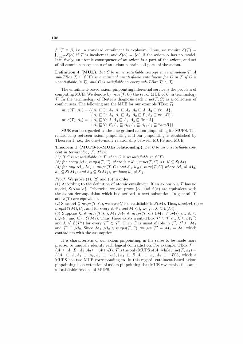
β, T � β, i.e., a standard entailment is explosive. Thus, we require E(T ) =⋃α∈T E(α) if T is incoherent, and E(α) = {α} if the axiom α has no model.

Intuitively, an atomic consequence of an axiom is a part of the axiom, and setof all atomic consequences of an axiom contains all parts of the axiom.

Definition 4 (MUE). Let C be an unsatisfiable concept in terminology T . Asub-TBox Tc ⊆ E(T ) is a minimal unsatisfiable entailment for C in T if C isunsatisfiable in Tc, and C is satisfiable in every sub-TBox T ′

c ⊂ Tc.The entailment-based axiom pinpointing inferential service is the problem of

computing MUE. We denote by mue(T , C) the set of MUE of C in terminologyT . In the terminology of Reiter’s diagnosis each mue(T , C) is a collection ofconflict sets. The following are the MUE for our example TBox T1:

mue(T1, A1) = {{A1 v ∃r.A2, A1 v A3, A2 v A,A3 v ∀r.¬A},{A1 v ∃r.A2, A1 v A3, A2 v B,A3 v ∀r.¬B}}

mue(T1, A4) = {{A4 v ∀r.A,A4 v A5, A5 v ∃r.¬A},{A4 v ∀s.B,A4 v A5, A5 v A6, A6 v ∃s.¬B}}

MUE can be regarded as the fine-grained axiom pinpointing for MUPS. Therelationship between axiom pinpointing and our pinpointing is established byTheorem 1, i.e., the one-to-many relationship between MUPS and MUE.

Theorem 1 (MUPS-to-MUEs relationship). Let C be an unsatisfiable con-cept in terminology T . Then:(1) If C is unsatisfiable in T , then C is unsatisfiable in E(T ).(2) for every M∈ mups(T , C), there is a K ∈ mue(T , C) s.t. K ⊆ E(M).(3) for any M1,M2 ∈ mups(T , C) and K1,K2 ∈ mue(T , C) where M1 6=M2,K1 ⊆ E(M1) and K2 ⊆ E(M2), we have K1 6= K2.

Proof. We prove (1), (2) and (3) in order.(1) According to the definition of atomic entailment, If an axiom α ∈ T has nomodel, E(α)={α}. Otherwise, we can prove {α} and E(α) are equivalent withthe axiom decomposition which is described in next subsection. In general, Tand E(T ) are equivalent.(2) SinceM⊆ mups(T , C), we have C is unsatisfiable in E(M). Thus,mue(M, C) =mups(E(M), C), and for every K ∈ mue(M, C), we get K ⊆ E(M).(3) Suppose K ∈ mue(T , C),M1,M2 ∈ mups(T , C) (M1 6= M2) s.t. K ⊆E(M1) and K ⊆ E(M2). Thus, there exists a sub-TBox T ′ ⊆ T s.t. K ⊆ E(T ′)and K * E(T ′′) for every T ′′ ⊂ T ′. Then C is unsatisfiable in T ′, T ′ ⊆ M1

and T ′ ⊆ M2. Since M1,M2 ∈ mups(T , C), we get T ′ = M1 = M2 whichcontradicts with the assumption.

It is characteristic of our axiom pinpointing, in the sense to be made moreprecise, to uniquely identify each logical contradiction. For example, TBox T ={A1 v AuBuA2, A2 v ¬Au¬B}, T is the only MUPS of A1 whilemue(T , A1) ={{A1 v A,A1 v A2, A2 v ¬A}, {A1 v B,A1 v A2, A2 v ¬B}}, which aMUPS has two MUE corresponding to. In this regard, entaiment-based axiompinpointing is an extension of axiom pinpointing that MUE covers also the sameunsatisfiable reasons of MUPS.

108

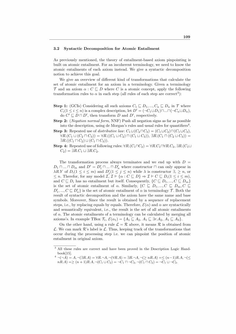
3.2 Syntactic Decomposition for Atomic Entailment

As previously mentioned, the theory of entailment-based axiom pinpointing isbuilt on atomic entailment. For an incoherent terminology, we need to know theatomic entailments of each axiom instead. We give a syntactic decompositionnotion to achieve this goal.

We give an overview of different kind of transformations that calculate theset of atomic entailment for an axiom in a terminology. Given a terminologyT and an axiom α : C v D where C is a atomic concept, apply the followingtransformation rules to α in each step (all rules of each step are correct3):

Step 1: (GCIs) Considering all such axioms C1 v D1, ..., Cn v Dn in T whereCi(1 ≤ i ≤ n) is a complex description, let D′ = (¬C1tD1)u...u(¬CntDn),do C ′ v D uD′, then transform D and D′, respectively.

Step 2: (Negation normal form, NNF) Push all negation signs as far as possibleinto the description, using de Morgan’s rules and usual rules for quantifiers4.

Step 3: Repeated use of distributive law : C1t(C2uC3) = (C1tC2)u(C1tC3),∀R.(C1 t (C2 u C3)) = ∀R.((C1 t C2) u (C1 t C3)), ∃R.(C1 u (C2 t C3)) =∃R.((C1 u C2) t (C1 u C3)).

Step 4: Repeated use of following rules: ∀R.(C1uC2) = ∀R.C1u∀R.C2, ∃R.(C1tC2) = ∃R.C1 t ∃R.C2.

The transformation process always terminates and we end up with D =D1 u ... uDm and D′ = D′

1 u ... uD′n where constructor u can only appear in

λR.Y of Di(1 ≤ i ≤ m) and D′j(1 ≤ j ≤ n) while λ is constructor ∃, ≥ n, or

≤ n. Therefor, for any model I, I � {α : C v D} ⇒ I � C v Di(1 ≤ i ≤ m),and C v Di has no entailment but itself. Consequently, {C v D1, ..., C v Dm}is the set of atomic entailment of α. Similarly, {C v D1, ..., C v Dm, C vD′

1, ..., C v D′n} is the set of atomic entailment of α in terminology T . Both the

result of syntactic decomposition and the axiom have the same name and basesymbols. Moreover, Since the result is obtained by a sequence of replacementsteps, i.e., by replacing equals by equals. Therefore, E(α) and α are syntacticallyand semantically equivalent, i.e., the result is the set of all atomic entailmentsof α. The atomic entailments of a terminology can be calculated by merging allaxioms’s. In example TBox T1, E(α1) = {A1 v A2, A1 v ∃r.A2, A1 v A3}.

On the other hand, using a rule L = R above, it means R is obtained fromL. We can mark R’s label is L. Thus, keeping track of the transformations thatoccur during the processing step i.e. we can pinpoint the position of atomicentailment in original axiom.

3 All these rules are correct and have been proved in the Description Logic Hand-book[15].

4 ¬(¬A) = A,¬(∃R.A) = ∀R.¬A,¬(∀R.A) = ∃R.¬A,¬(≥ nR.A) =≤ (n−1)R.A,¬(≤nR.A) =≥ (n+ 1)R.A,¬(C1 t C2) = ¬C1 u ¬C2,¬(C1 u C2) = ¬C1 t ¬C2.

109

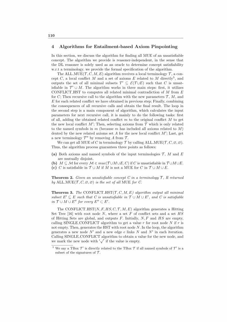
4 Algorithms for Entailment-based Axiom Pinpointing

In this section, we discuss the algorithm for finding all MUE of an unsatisfiableconcept. The algorithm we provide is reasoner-independent, in the sense thatthe DL reasoner is solely used as an oracle to determine concept satisfiabilityw.r.t a terminology. we provide the formal specification of the algorithm.

The ALL MUE(T , C,M,E) algorithm receives a local terminology T , a con-cept C, a local conflict M and a set of axioms E related to M directly5, andoutputs the set of all minimal subsets T ′ ⊆ E(T ∪E) such that C is unsat-isfiable in T ′ ∪ M . The algorithm works in three main steps: first, it utilizesCONFLICT HST to computes all related minimal contradiction of M from Efor C; Then recursive call to the algorithm with the new parameters T , M , andE for each related conflict we have obtained in previous step; Finally, combiningthe consequences of all recursive calls and obtain the final result. The loop inthe second step is a main component of algorithm, which calculates the inputparameters for next recursive call, it is mainly to do the following tasks: firstof all, adding the obtained related conflict m to the original conflict M to getthe new local conflict M ′; Then, selecting axioms from T which is only relatedto the named symbols in m (because m has included all axioms related to M)dented by the new related axioms set A for the new local conflict M ′; Last, geta new terminology T ′′ by removing A from T .

We can get all MUE of C in terminology T by calling ALL MUE(T , C,∅,∅).Thus, the algorithm process guarantees three points as follows:

(a) Both axioms and named symbols of the input terminologies T , M and Eare mutually disjoint.

(b) M ⊆M for everyM∈ mue(T ∪M∪E,C) if C is unsatisfiable in T ∪M∪E.(c) C is satisfiable in T ∪M if M is not a MUE for C in T ∪M ∪ E.

Theorem 2. Given an unsatisfiable concept C in a terminology T , R returnedby ALL MUE(T , C,∅,∅) is the set of all MUE for C.

Theorem 3. The CONFLICT HST(T , C,M,E) algorithm output all minimalsubset E′ ⊆ E such that C is unsatisfiable in T ∪M ∪ E′, and C is satisfiablein T ∪M ∪ E′′ for every E′′ ⊂ E′.

The CONFLICT HST(N,F,HS,C, T ,M,E) algorithm generates a HittingSet Tree [16] with root node N , where a set F of conflict sets and a set HSof Hitting Sets are global, and outputs F . Initially, N,F and HS are empty,calling SINGLE CONFLICT algorithm to get a value r for root node N if r isnot empty. Then, generates the HST with root nodeN . In the loop, the algorithmgenerates a new node N ′ and a new edge e links N and N ′ in each iteration.Calling SINGLE CONFLICT algorithm to obtain a value for the new node, andwe mark the new node with ′√′

if the value is empty.

5 We say a TBox T ′ is directly related to the TBox T if all named symbols of T ′ is asubset of the signatures of T .

110

Algorithm: ALL MUE(T , C,M,E)Input: a terminology T , a concept C, a terminology M , a terminology EOutput: all minimal subsets of E(T ∪E) conflict with M w.r.t. C R

R ← ∅;T ′ ← T ;E′ ← E;if M = ∅ then /* The algorithm start with M = ∅ */

A← {α ∈ T |α has the form C v D};T ′ ← T −A;E′ ← E(A);

if C is unsatisfiable in M then /* M is a MUE of C */R← {M};return R;

H ← ∅;CONFLICT HST(∅, H,∅, C, T ′,M,E′);if H = ∅ then /* H = ∅ means M is a MUE of C */

R← {M};return R;

for m ∈ H doM ′ ←M ∪m; /* update the current MUE M of C */S ← Sig(m)−D(M ′)− B(T ′ ∪M ′);/*Select the related symbols of M ′*/A← {α ∈ T ′ |α has the form C′ v D′ where C′ ∈ S};T ′′ ← T ′ −A;R′ ← ALL MUE(T ′′, C,M ′, E(A));R← R ∪R′;

return R;

Two pruning strategy to the algorithm in order to reduce the size of HST andeliminate extraneous satisfiability tests. One is closing, if there exists a HittingSet h in HS such that the path of N ′ is a superset of h, close node N ′ and thevalue is not computed for N ′ nor are any succor nodes generated, as indicted bya ′×′. The other one is reusing nodes: if there exists a node value k in F suchthat k and the path of N ′ are disjoint, set k as the value of N ′ directly withoutrecalculation.

The SINGLE CONFLICT(T , C,M,E) algorithm outputs a subset of E. Inthe loop, the algorithm removes an axiom from E in each iteration and checkwhether the concept C is satisfiable w.r.t. T ∪M ∪ E, in which case the axiomis added to R and reinserted into E. The process continues until all axioms inE have been tested. Finally, R is returned as output.

Theorem 4. The SINGLE CONFLICT(T , C,M,E) algorithm output a mini-mal subset R ⊆ E such that C is unsatisfiable in T ∪M ∪R, and C is satisfiablein T ∪M ∪R′ for every R′ ⊂ R.

Proof. Let R be the output of algorithm SINGLE CONFLICT(T , C,M,E). IfC is satisfiable in T ∪M ∪ E, we get R = ∅. Otherwise, C is unsatisfiable inT ∪M ∪ R upon termination. Suppose there exists a subset R′ ⊂ R such thatC is unsatisfiable in T ∪M ∪R′. Then, removing the axiom in R−R′ after the

111

Algorithm: CONFLICT HST(N,F,HS, T , C,M,E)Input: a node N , a set of conflict sets F , a set of hitting sets HS,

a terminology T , a concept C, a terminology M , a terminology EOutput: input F

if N = ∅ thenr ←SINGLE CONFLICT(T , C,M,E);if r = ∅ then

return;L(N)← r;F ← {r};

for α ∈ L(N) docreate a new node N ′ and set L(N ′)← ∅;create a new edge e =< N,N ′ > with L(e)← α;if there exists a set h ∈ HS s.t. h ⊆ P(N) ∪ {α} thenL(N ′)←′ × ′;continue;

else if there exists a set k ∈ F s.t. k ∩ P(N) = ∅ thenL(N ′)← k;CONFLICT HST(N ′, F,HS, T , C,M,E − {α});

elsem← SINGLE CONFLICT(T , C,M,E − {α});if m = ∅ thenL(N ′)←′ √ ′;HS ← HS ∪ {P(N) ∪ {α}};

elseL(N ′)← m;F ← F ∪ {m};CONFLICT HST(N ′, F,HS, T , C,M,E − {α});

removal of R′, we get C is satisfiable in T ∪M ∪R′, which contradicts with theassumption.

Algorithm: SINGLE CONFLICT(T , C,M,E)Input: a terminology T , a concept C, a terminology M , a terminologyEOutput: a set of axioms (a subset of E) R

R ← ∅;T ′ ← T ∪M ∪ E;if (C is satisfiable in T ′) then

return R;for α ∈ E doT ′ ← T ′ − {α};if C is satisfiable in T ′ thenT ′ ← T ′ ∪ {α};R← R ∪ {α};

return R;

112

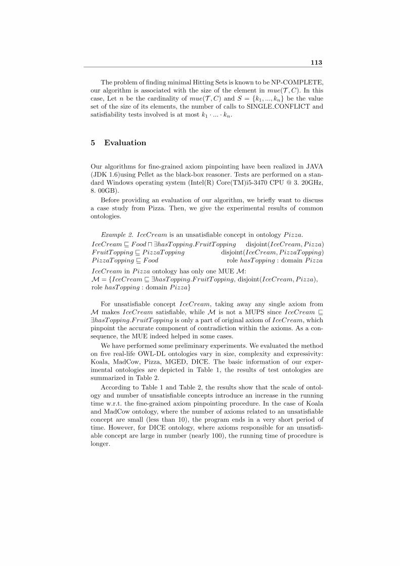
The problem of finding minimal Hitting Sets is known to be NP-COMPLETE,our algorithm is associated with the size of the element in mue(T , C). In thiscase, Let n be the cardinality of mue(T , C) and S = {k1, ..., kn} be the valueset of the size of its elements, the number of calls to SINGLE CONFLICT andsatisfiability tests involved is at most k1 · ... · kn.

5 Evaluation

Our algorithms for fine-grained axiom pinpointing have been realized in JAVA(JDK 1.6)using Pellet as the black-box reasoner. Tests are performed on a stan-dard Windows operating system (Intel(R) Core(TM)i5-3470 CPU @ 3. 20GHz,8. 00GB).

Before providing an evaluation of our algorithm, we briefly want to discussa case study from Pizza. Then, we give the experimental results of commonontologies.

Example 2. IceCream is an unsatisfiable concept in ontology Pizza.

IceCream v Food u ∃hasTopping.FruitTopping disjoint(IceCream,P izza)FruitTopping v PizzaTopping disjoint(IceCream,P izzaTopping)PizzaTopping v Food role hasTopping : domain Pizza

IceCream in Pizza ontology has only one MUE M:M = {IceCream v ∃hasTopping.FruitTopping, disjoint(IceCream,P izza),role hasTopping : domain Pizza}

For unsatisfiable concept IceCream, taking away any single axiom fromM makes IceCream satisfiable, while M is not a MUPS since IceCream v∃hasTopping.FruitTopping is only a part of original axiom of IceCream, whichpinpoint the accurate component of contradiction within the axioms. As a con-sequence, the MUE indeed helped in some cases.

We have performed some preliminary experiments. We evaluated the methodon five real-life OWL-DL ontologies vary in size, complexity and expressivity:Koala, MadCow, Pizza, MGED, DICE. The basic information of our exper-imental ontologies are depicted in Table 1, the results of test ontologies aresummarized in Table 2.

According to Table 1 and Table 2, the results show that the scale of ontol-ogy and number of unsatisfiable concepts introduce an increase in the runningtime w.r.t. the fine-grained axiom pinpointing procedure. In the case of Koalaand MadCow ontology, where the number of axioms related to an unsatisfiableconcept are small (less than 10), the program ends in a very short period oftime. However, for DICE ontology, where axioms responsible for an unsatisfi-able concept are large in number (nearly 100), the running time of procedure islonger.

113

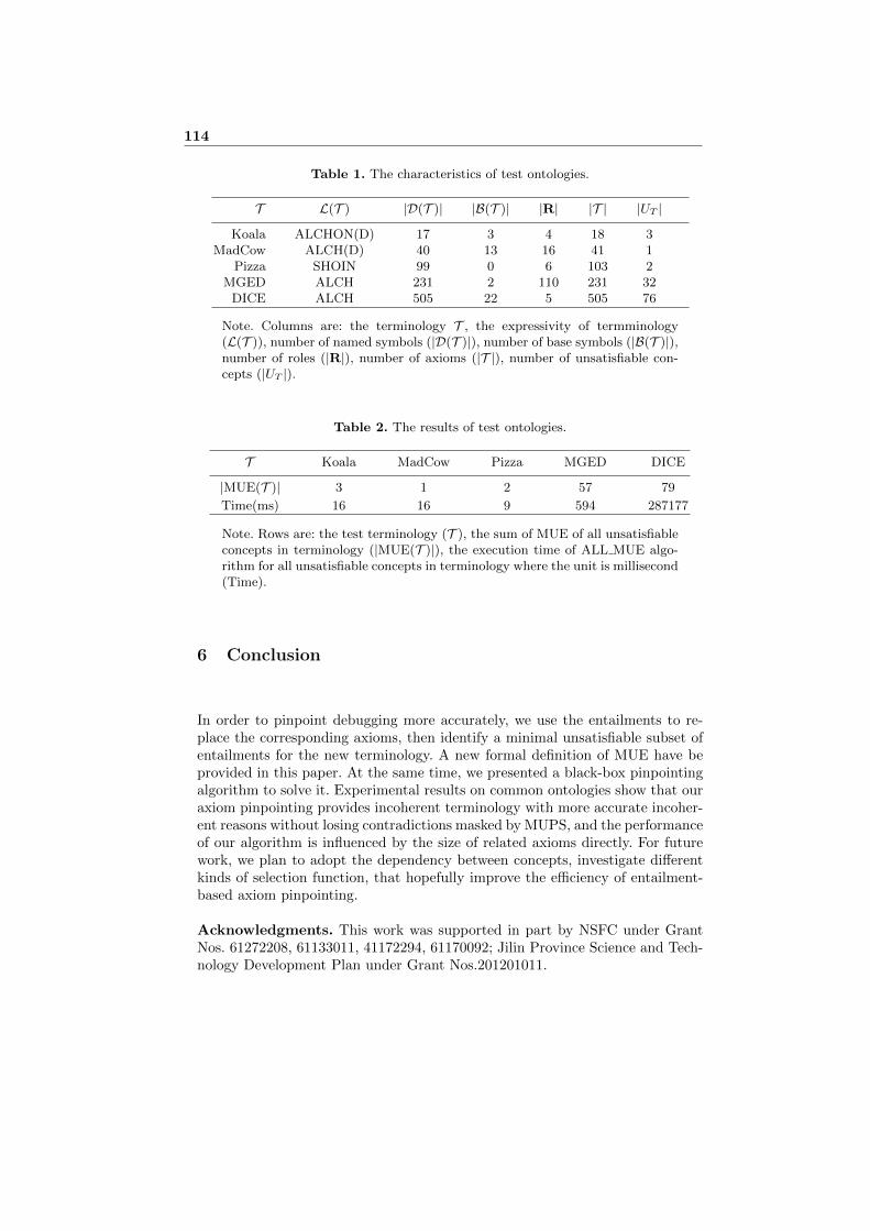
Table 1. The characteristics of test ontologies.

T L(T ) |D(T )| |B(T )| |R| |T | |UT |Koala ALCHON(D) 17 3 4 18 3

MadCow ALCH(D) 40 13 16 41 1Pizza SHOIN 99 0 6 103 2

MGED ALCH 231 2 110 231 32DICE ALCH 505 22 5 505 76

Note. Columns are: the terminology T , the expressivity of termminology(L(T )), number of named symbols (|D(T )|), number of base symbols (|B(T )|),number of roles (|R|), number of axioms (|T |), number of unsatisfiable con-cepts (|UT |).

Table 2. The results of test ontologies.

T Koala MadCow Pizza MGED DICE

|MUE(T )| 3 1 2 57 79

Time(ms) 16 16 9 594 287177

Note. Rows are: the test terminology (T ), the sum of MUE of all unsatisfiableconcepts in terminology (|MUE(T )|), the execution time of ALL MUE algo-rithm for all unsatisfiable concepts in terminology where the unit is millisecond(Time).

6 Conclusion

In order to pinpoint debugging more accurately, we use the entailments to re-place the corresponding axioms, then identify a minimal unsatisfiable subset ofentailments for the new terminology. A new formal definition of MUE have beprovided in this paper. At the same time, we presented a black-box pinpointingalgorithm to solve it. Experimental results on common ontologies show that ouraxiom pinpointing provides incoherent terminology with more accurate incoher-ent reasons without losing contradictions masked by MUPS, and the performanceof our algorithm is influenced by the size of related axioms directly. For futurework, we plan to adopt the dependency between concepts, investigate differentkinds of selection function, that hopefully improve the efficiency of entailment-based axiom pinpointing.

Acknowledgments. This work was supported in part by NSFC under GrantNos. 61272208, 61133011, 41172294, 61170092; Jilin Province Science and Tech-nology Development Plan under Grant Nos.201201011.

114

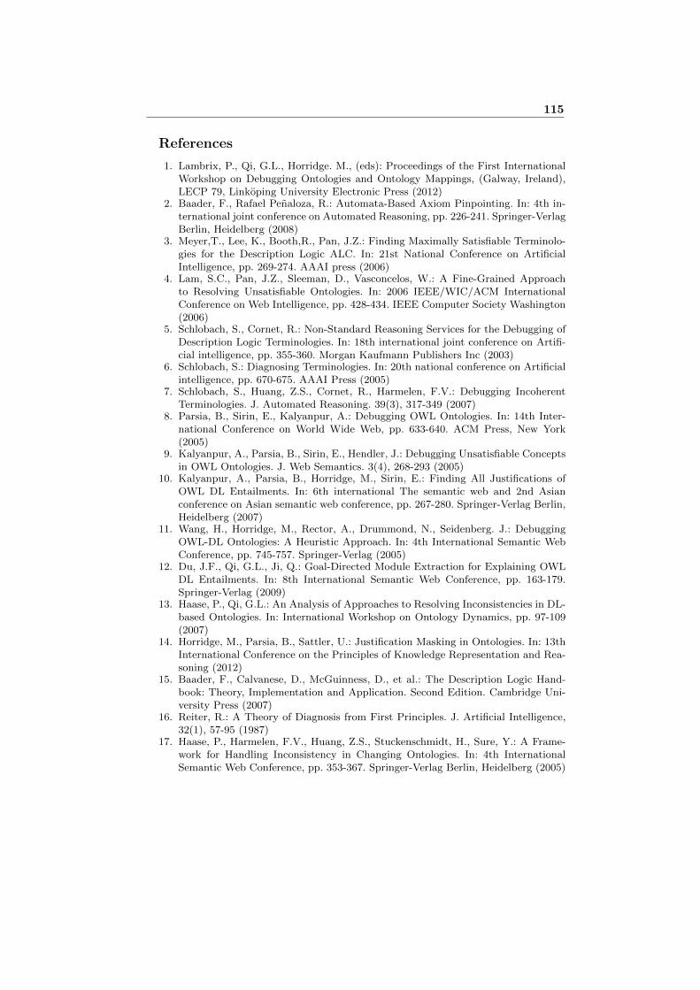
References

1. Lambrix, P., Qi, G.L., Horridge. M., (eds): Proceedings of the First InternationalWorkshop on Debugging Ontologies and Ontology Mappings, (Galway, Ireland),LECP 79, Linkoping University Electronic Press (2012)

2. Baader, F., Rafael Penaloza, R.: Automata-Based Axiom Pinpointing. In: 4th in-ternational joint conference on Automated Reasoning, pp. 226-241. Springer-VerlagBerlin, Heidelberg (2008)

3. Meyer,T., Lee, K., Booth,R., Pan, J.Z.: Finding Maximally Satisfiable Terminolo-gies for the Description Logic ALC. In: 21st National Conference on ArtificialIntelligence, pp. 269-274. AAAI press (2006)

4. Lam, S.C., Pan, J.Z., Sleeman, D., Vasconcelos, W.: A Fine-Grained Approachto Resolving Unsatisfiable Ontologies. In: 2006 IEEE/WIC/ACM InternationalConference on Web Intelligence, pp. 428-434. IEEE Computer Society Washington(2006)

5. Schlobach, S., Cornet, R.: Non-Standard Reasoning Services for the Debugging ofDescription Logic Terminologies. In: 18th international joint conference on Artifi-cial intelligence, pp. 355-360. Morgan Kaufmann Publishers Inc (2003)

6. Schlobach, S.: Diagnosing Terminologies. In: 20th national conference on Artificialintelligence, pp. 670-675. AAAI Press (2005)

7. Schlobach, S., Huang, Z.S., Cornet, R., Harmelen, F.V.: Debugging IncoherentTerminologies. J. Automated Reasoning. 39(3), 317-349 (2007)

8. Parsia, B., Sirin, E., Kalyanpur, A.: Debugging OWL Ontologies. In: 14th Inter-national Conference on World Wide Web, pp. 633-640. ACM Press, New York(2005)

9. Kalyanpur, A., Parsia, B., Sirin, E., Hendler, J.: Debugging Unsatisfiable Conceptsin OWL Ontologies. J. Web Semantics. 3(4), 268-293 (2005)

10. Kalyanpur, A., Parsia, B., Horridge, M., Sirin, E.: Finding All Justifications ofOWL DL Entailments. In: 6th international The semantic web and 2nd Asianconference on Asian semantic web conference, pp. 267-280. Springer-Verlag Berlin,Heidelberg (2007)

11. Wang, H., Horridge, M., Rector, A., Drummond, N., Seidenberg. J.: DebuggingOWL-DL Ontologies: A Heuristic Approach. In: 4th International Semantic WebConference, pp. 745-757. Springer-Verlag (2005)

12. Du, J.F., Qi, G.L., Ji, Q.: Goal-Directed Module Extraction for Explaining OWLDL Entailments. In: 8th International Semantic Web Conference, pp. 163-179.Springer-Verlag (2009)

13. Haase, P., Qi, G.L.: An Analysis of Approaches to Resolving Inconsistencies in DL-based Ontologies. In: International Workshop on Ontology Dynamics, pp. 97-109(2007)

14. Horridge, M., Parsia, B., Sattler, U.: Justification Masking in Ontologies. In: 13thInternational Conference on the Principles of Knowledge Representation and Rea-soning (2012)

15. Baader, F., Calvanese, D., McGuinness, D., et al.: The Description Logic Hand-book: Theory, Implementation and Application. Second Edition. Cambridge Uni-versity Press (2007)

16. Reiter, R.: A Theory of Diagnosis from First Principles. J. Artificial Intelligence,32(1), 57-95 (1987)

17. Haase, P., Harmelen, F.V., Huang, Z.S., Stuckenschmidt, H., Sure, Y.: A Frame-work for Handling Inconsistency in Changing Ontologies. In: 4th InternationalSemantic Web Conference, pp. 353-367. Springer-Verlag Berlin, Heidelberg (2005)

115

An automatic way of generating incoherentterminologies with parameters

Yu Zhang, Dantong Ouyang, and Yuxin Ye ?

College of Computer Science and Technology,Jilin University, Changchun 130012, China

Abstract. The minimal incoherence preserving sub-terminologies (Mip-s) is defined for identifying the axioms responsible for the unsatisfiableconcepts in incoherent ontology. While a great many performance evalu-ations have been proposed in the past, what remains to be investigatedis whether we have effective reasoners to solve the Mips problems, inwhich case a particular reasoner will be more efficiency than others.After analyzing the structural complexity of terminology, we develop aMips Benchmark (MipsBM) to evaluate the performances of reasoners bydefining six complexity metrics based on concept dependency network-s model. Evaluation experiments show that the proposed metrics caneffectively reflect the complexity of benchmark data. Not only can thebenchmark help the users to determine which reasoner is likely to per-form best in their applications, but also help the developers to improvethe performances and qualities of their reasoners.

Keywords: Incoherent terminology; Mips; Benchmark; MipsBM

1 Introduction

In practice, building an ontology is a very complicated process and is easy tomake errors, an ontology O is incoherent if there exists an unsatisfiable conceptin O, and the existence of unsatisfiable concept indicates that the formal def-inition is incorrect. Therefore, how to find all the unsatisfiable concepts is thechallenging of ontology debugging. Researchers have proposed various methodsto debug incoherent ontology. Ontology debugging is achieved by using reason-ers, currently, most of the reasoners, such as Pellet [1], HermiT[2], FaCT++[3],TrOWL[4] and JFact support the inference tasks. A great many performanceevaluations for reasoners have been performed in the past, What remains to beinvestigated is whether we have effective reasoners to solve the Mips problems,in which cases a particular reasoner will be more efficiency than others. Thereare several criteria for a good benchmark test data. First, we need to system-atically construct several types of logical contradictions to create an incoherentTBox. Second, there must be a number of parameters that could influence thecomplexity of benchmark data and the difficulty for reasoning.

? corresponding author: yeyx@jlu.edu.cn (Yuxin Ye).

2 Related Work

In the research of knowledge base query, (LUBM) [5] is developed based on sev-eral complexity metrics of ontology and provides 14 test queries to assess theefficiency, correctness and completeness of the knowledge base. However, the cor-relations between the classes of LUBM are low, thus Li Ma extends it to Univer-sity Ontology Benchmark (UOBM) [6] by adding a series of association classes.However, either LUBM or UOBM only can evaluate single ontology, thus YingjieLi et al. [7] develop a multi-ontology synthetic benchmark that can evaluate notonly single ontology but also federated ontologies. In the research of ontologymatching, Alfio Ferrara et al. [8] propose a disciplined approach to the semi-automatic generation of benchmarks called SWING (Semantic Web InstanceGeneration), but all the evaluations in SWING are only for single language, soChristian Meilicke et al. [9] design a benchmark for multilingual ontology match-ing called MultiFarm. Besides, the work in [10] presents the design of a modulartest generator to evaluate different matchers on the generated tests. In the re-search of ontology reasoning and debugging, the benchmarks proposed in [11]and [12] are used to evaluate the classification performances of reasoners. Thework in [13] focus on the applicability of specific reasoners to certain expressivi-ty clusters, and evaluate the loading time, classification and conjunctive queriesperformances of reasoners. JustBench [14] is a typical benchmark to evaluatethe reasoners for calcuating justification. In [15], several machine learning tech-niques are used to predict classification time and determine the metrics that canbe used to predict reasoning performance. The work in [16] proposes a methodto construct the justification dataset from realistic ontologies with different sizesand expressivities.

3 Complexity Analysis for Incoherent TBox

The expressivity of a particular DL is determined by the concept constructors itprovides [17]. SHOIN (D) is a very expressive DL that provides the constructorsincluding H (role hierarchies), O(nominals), I(inverse roles), N (Number restric-tion) and S is the abbreviation forALC with transitive roles.ALC is the basic de-scription logic consisting of the constructors ¬C (negation), CuD(conjunction),C tD(disjunction), ∃r.C(existential restriction) and ∀r.C(value restriction).

Example 1. Suppose a SHOIN (D) TBox contains the following axioms:α1 : S1 ≡ ∃r1.B1, α2 : S2 ≡ ∀r2.B2, α3 : S3 ≡ {B2} t {B3},α4 : S4 v S1 t S2, α5 : S5 v ∃r4.S3 u S4, α6 : S6 ≡ ∃r5.B4,α7 : S7 ≡ {B4} t {B5}, α8 : S8 v ∃r6.S6 u S7, α9 : C1 ≡ ∀t1.¬A1,α10 : C2 ≡ ∃t1.A1u∀t2.A2, α11 : C3 ≡ ∀t2.A2u∃t2.¬A2, α12 : C4 ≡ ∃t2.¬A2,α13 : C5 ≡≥ 3t3u ≤ 2t3, α14 : C6 v C1 u C2, α15 : C7 v C2,α16 : C8 v C4, α17 : C9 v C7 u C8, α18 : C10 v C5 u C6 u C9,α19 : r1 ≡ r−4 , α20 : r2 v r3, α21 : r5 ◦ r5 v r5

118

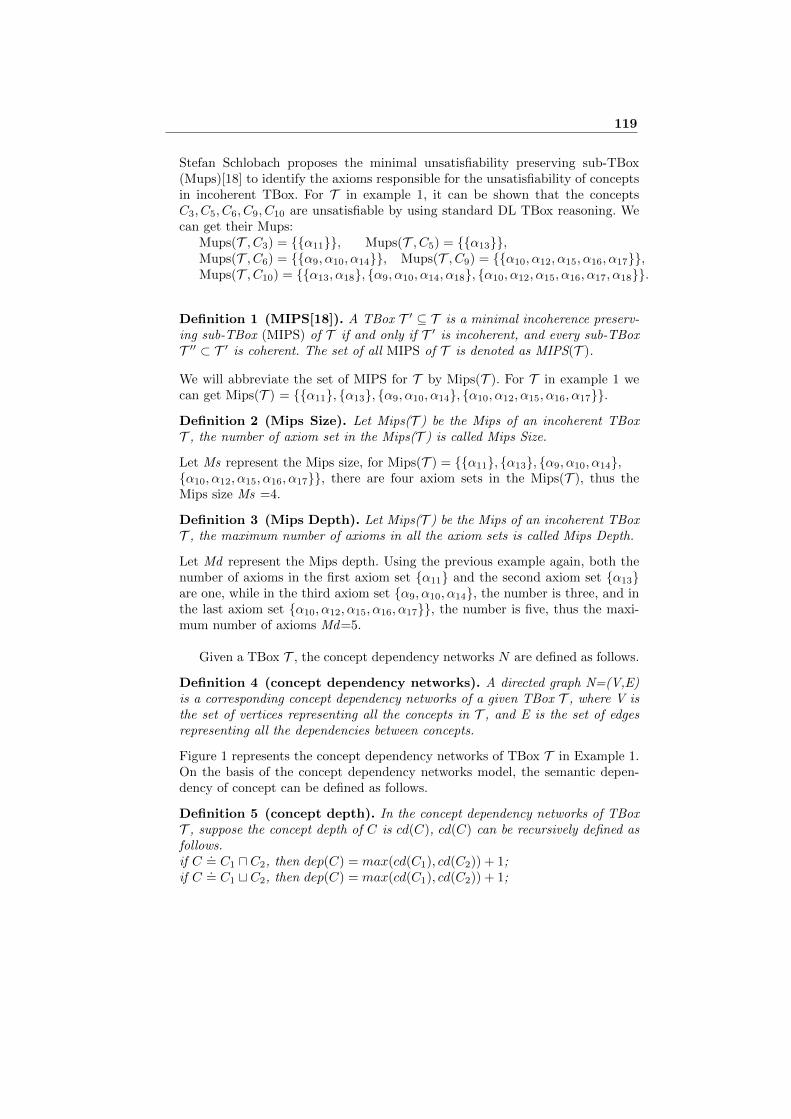
Stefan Schlobach proposes the minimal unsatisfiability preserving sub-TBox(Mups)[18] to identify the axioms responsible for the unsatisfiability of conceptsin incoherent TBox. For T in example 1, it can be shown that the conceptsC3, C5, C6, C9, C10 are unsatisfiable by using standard DL TBox reasoning. Wecan get their Mups:

Mups(T , C3) = {{α11}}, Mups(T , C5) = {{α13}},Mups(T , C6) = {{α9, α10, α14}}, Mups(T , C9) = {{α10, α12, α15, α16, α17}},Mups(T , C10) = {{α13, α18}, {α9, α10, α14, α18}, {α10, α12, α15, α16, α17, α18}}.

Definition 1 (MIPS[18]). A TBox T ′ ⊆ T is a minimal incoherence preserv-ing sub-TBox (MIPS) of T if and only if T ′ is incoherent, and every sub-TBoxT ′′ ⊂ T ′ is coherent. The set of all MIPS of T is denoted as MIPS(T ).

We will abbreviate the set of MIPS for T by Mips(T ). For T in example 1 wecan get Mips(T ) = {{α11}, {α13}, {α9, α10, α14}, {α10, α12, α15, α16, α17}}.

Definition 2 (Mips Size). Let Mips(T ) be the Mips of an incoherent TBoxT , the number of axiom set in the Mips(T ) is called Mips Size.

Let Ms represent the Mips size, for Mips(T ) = {{α11}, {α13}, {α9, α10, α14},{α10, α12, α15, α16, α17}}, there are four axiom sets in the Mips(T ), thus theMips size Ms =4.

Definition 3 (Mips Depth). Let Mips(T ) be the Mips of an incoherent TBoxT , the maximum number of axioms in all the axiom sets is called Mips Depth.

Let Md represent the Mips depth. Using the previous example again, both thenumber of axioms in the first axiom set {α11} and the second axiom set {α13}are one, while in the third axiom set {α9, α10, α14}, the number is three, and inthe last axiom set {α10, α12, α15, α16, α17}}, the number is five, thus the maxi-mum number of axioms Md=5.

Given a TBox T , the concept dependency networks N are defined as follows.

Definition 4 (concept dependency networks). A directed graph N=(V,E)is a corresponding concept dependency networks of a given TBox T , where V isthe set of vertices representing all the concepts in T , and E is the set of edgesrepresenting all the dependencies between concepts.

Figure 1 represents the concept dependency networks of TBox T in Example 1.On the basis of the concept dependency networks model, the semantic depen-dency of concept can be defined as follows.

Definition 5 (concept depth). In the concept dependency networks of TBoxT , suppose the concept depth of C is cd(C), cd(C) can be recursively defined asfollows.if C

.= C1 u C2, then dep(C) = max(cd(C1), cd(C2)) + 1;

if C.= C1 t C2, then dep(C) = max(cd(C1), cd(C2)) + 1;

119

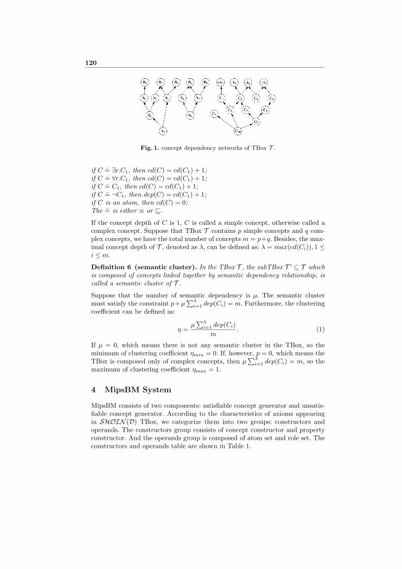
Fig. 1. concept dependency networks of TBox T .

if C.= ∃r.C1, then cd(C) = cd(C1) + 1;

if C.= ∀r.C1, then cd(C) = cd(C1) + 1;

if C.= C1, then cd(C) = cd(C1) + 1;

if C.= ¬C1, then dep(C) = cd(C1) + 1;

if C is an atom, then cd(C) = 0;The

.= is either ≡ or v.

If the concept depth of C is 1, C is called a simple concept, otherwise called acomplex concept. Suppose that TBox T contains p simple concepts and q com-plex concepts, we have the total number of concepts m = p+q. Besides, the max-imal concept depth of T , denoted as λ, can be defined as: λ = max(cd(Ci)), 1 ≤i ≤ m.

Definition 6 (semantic cluster). In the TBox T , the subTBox T ′ ⊆ T whichis composed of concepts linked together by semantic dependency relationship, iscalled a semantic cluster of T .

Suppose that the number of semantic dependency is µ. The semantic clustermust satisfy the constraint p+µ

∑λi=1 dep(Ci) = m. Furthermore, the clustering

coefficient can be defined as:

η =µ∑λi=1 dep(Ci)

m. (1)

If µ = 0, which means there is not any semantic cluster in the TBox, so theminimum of clustering coefficient ηmin = 0. If, however, p = 0, which means theTBox is composed only of complex concepts, then µ

∑λi=1 dep(Ci) = m, so the

maximum of clustering coefficient ηmax = 1.

4 MipsBM System

MipsBM consists of two components: satisfiable concept generator and unsatis-fiable concept generator. According to the characteristics of axioms appearingin SHOIN (D) TBox, we categorize them into two groups: constructors andoperands. The constructors group consists of concept constructor and propertyconstructor. And the operands group is composed of atom set and role set. Theconstructors and operands table are shown in Table 1.

120

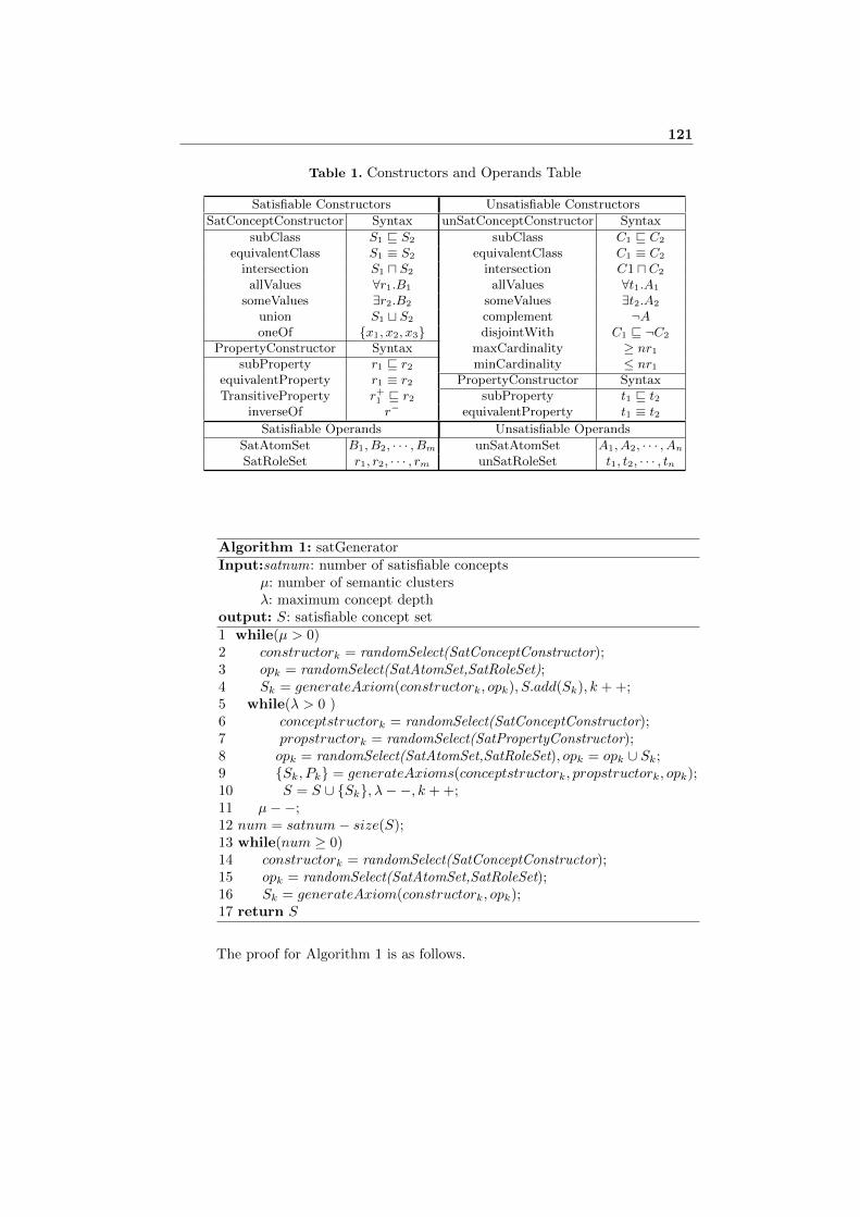
Table 1. Constructors and Operands Table

Satisfiable Constructors Unsatisfiable Constructors

SatConceptConstructor Syntax unSatConceptConstructor Syntax

subClass S1 v S2 subClass C1 v C2

equivalentClass S1 ≡ S2 equivalentClass C1 ≡ C2

intersection S1 u S2 intersection C1 u C2

allValues ∀r1.B1 allValues ∀t1.A1

someValues ∃r2.B2 someValues ∃t2.A2

union S1 t S2 complement ¬AoneOf {x1, x2, x3} disjointWith C1 v ¬C2

PropertyConstructor Syntax maxCardinality ≥ nr1subProperty r1 v r2 minCardinality ≤ nr1

equivalentProperty r1 ≡ r2 PropertyConstructor SyntaxTransitiveProperty r+1 v r2 subProperty t1 v t2

inverseOf r− equivalentProperty t1 ≡ t2Satisfiable Operands Unsatisfiable Operands

SatAtomSet B1, B2, · · · , Bm unSatAtomSet A1, A2, · · · , An

SatRoleSet r1, r2, · · · , rm unSatRoleSet t1, t2, · · · , tn

Algorithm 1: satGeneratorInput:satnum: number of satisfiable concepts

µ: number of semantic clustersλ: maximum concept depth

output: S: satisfiable concept set1 while(µ > 0)2 constructork = randomSelect(SatConceptConstructor);3 opk = randomSelect(SatAtomSet,SatRoleSet);4 Sk = generateAxiom(constructork, opk), S.add(Sk), k + +;5 while(λ > 0 )6 conceptstructork = randomSelect(SatConceptConstructor);7 propstructork = randomSelect(SatPropertyConstructor);8 opk = randomSelect(SatAtomSet,SatRoleSet), opk = opk ∪ Sk;9 {Sk, Pk} = generateAxioms(conceptstructork, propstructork, opk);10 S = S ∪ {Sk}, λ−−, k + +;11 µ−−;12 num = satnum− size(S);13 while(num ≥ 0)14 constructork = randomSelect(SatConceptConstructor);15 opk = randomSelect(SatAtomSet,SatRoleSet);16 Sk = generateAxiom(constructork, opk);17 return S

The proof for Algorithm 1 is as follows.

121

Proof. Because there are not any complement or disjoint constructors in theSatisfiable Constructors in Table 1, the concepts generated by Algorithm 1 mustbe satisfiable.

The first while loop corresponds to the number of semantic clusters, in eachloop, the algorithm creates a semantic cluster, and the value of µ is decreasedby 1 until µ = 0. The second while loop corresponds to the maximum conceptdepth, in each loop, the algorithm creates a concept, and the concept depth ofthe latter concept is 1 bigger than that of the former one. When the loop isfinished, the concept depth of the last concept reaches λ. After that, the numberof satisfiable concepts is obtained, the rest of the concepts are created in thethird while loop.

In order to build an incoherent terminology, MipsBM needs to create severalunsatisfiable concepts which can be achieved through systematically constructinglogical clashes.

Definition 7 (Independent Unsatisfiable Concept). C is an independentunsatisfiable concept if the unsatisfiability of C depends on the concept definitionrather than the unsatisfiability of other concepts.

Definition 8 (Dependent Unsatisfiable Concept). C is a dependent un-satisfiable concept if the unsatisfiability of C depends on the unsatisfiability ofother concepts.

From the Example 1, C3, C5, C6 and C9 are independent unsatisfiable concepts,C10 is dependent unsatisfiable concept because its unsatisfiability depends onunsatisfiable concepts C5, C6, C9.

Definition 9 (Clash Sequences). Let Seq+(C) be the positive clash sequenceof C, and Seq−(C) the negative clash sequence. Seq+(C) is of the form < (C1, I1, C2), (C2, I2, C3), · · · , (Cm, Im, C) > (i = 1, · · · ,m), where Ci v Ci−1, Ii repre-sents the indexes of axioms related to Ci v Ci−1. Seq−(C) is of the form< (¬C1, I

′1, C

′2), (C ′2, I

′2, C

′3), · · · , (C ′n, I ′n, C) > (i = 1, · · · , n), where C ′i v C ′i−1 ,

I ′i represents the indexes of axioms related to C ′i v C ′i−1. After that, the unsat-isfiable concept C can be generated by C v Cm u C ′n.

For example, The clash sequences of C9:Seq+(C9)=< (A1, {α10}, C2), (C2, {α10, α15}, C7), (C7, {α10, α15, α17}, C9)) >,Seq−(C9)=< (¬A1, {α12}, C4), (C4, {α12, α16}, C8), (C8, {α12, α16, α17}, C9) >.Unsatisfiable concepts can be divided into two types as follows.complement clash: C is a complement clash concept if it is a subclass of both

class A and the complement of class A. For example:α1 : C1 v ∀t1.A1 u ∃t1.¬A1. Then C1 is a complement clash root concept.cardinality clash: C is a cardinality clash concept if the at-least restriction is

bigger than the at-most restriction in its definition. For example:α2 : C2 ≡≥ 2.t2u ≤ 1.t2. Then C2 is a cardinality clash root concept.Unsatisfiable concept generator (Algorithm 2) creates the satisfiable concepts

by constructing clash sequences.

122

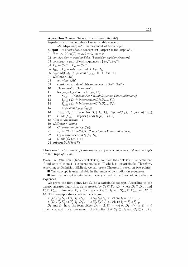
Algorithm 2: unsatGenerator(unsatnum,Ms,iMd)inputs:unsatnum: number of unsatisfiable concept

Ms: Mips size; iMd : increasement of Mips depthoutput: U : unsatisfiable concept set; Mips(T ): the Mips of T01 U = ∅, Mips(T ) = ∅, k = 0, len = 0;02 constructor = randomSelect(UnsatConceptConstructor;)03 construct a pair of clsh sequences : {Seq+,Seq+}04 D0 ← Seq+, D′0 ← Seq−;05 I(Ck) : Ck

.= intersectionOf(D0, D

′0);

06 CR.add(Ck), Mips.add(I(Ck)), k++, len++;07 while(k ≤ Ms)08 len=len+iMd;09 construct a pair of clsh sequences : {Seq+,Seq+}10 D0 ← Seq+, D′0 ← Seq−;11 for(i=j=1; j < len; i++,j=j+2)12 Sx,y ← (SatAtomSet,SatRoleSet,someValues,allValues);13 I(Di) : Di

.= intersectionOf(Di−1, Sx);

14 I ′(D′i)

: D′i.= intersectionOf(D′i−1, Sy);

15 Mips.add(I(Di), I′(D′

i));

16 I(Ck) : Ck.= intersectionOf(Di, D

′i), CR.add(Ck), Mips.add(I(Ck));

17 U .add(CR), Mips(T ).add(Mips), k++;18 num = unsatnum− k;19 while(m ≤ num)20 Cr ←randomSelect(CR);21 Sz ← (SatAtomSet,SatRoleSet,someValues,allValues);22 Ck

.= intersectionOf(Cr, Sz);

23 U .add(Ck),m+ +;24 return U,Mips(T )

Theorem 1 The unions of clash sequences of independent unsatisfiable conceptsare the Mips of TBox.

Proof. By Definition 1(Incoherent TBox), we have that a TBox T is incoherentif and only if there is a concept name in T which is unsatisfiable. Therefore,according to Definition 3(Mips), we can prove Theorem 1 based on two points:

� One concept is unsatisfiable in the union of contradiction sequences.� And the concept is satisfiable in every subset of the union of contradiction

sequences.We prove the first point. Let Ck be a satisfiable concept, According to the

unsatGenerator algorithm, Ck is created by Ck v DiuD′i, where Di v Di−1 andD′i v D′i−1 . Similarly, Di−1 v Di−2, · · · , D2 v D1 and D′i−1 v D′i−2, · · · , D′2 vD′1. The corresponding clash sequences are:

< (D1, I1, D2), (D2, I2, D3), · · · , (Di, Ii, Ck) >, where Ii = Ii ∪ Ii−1.< (D′1, I

′1, D

′2), (D′2, I

′2, D

′3), · · · , (D′i, I ′i, Ck) >, where I ′i = I ′i ∪ I ′i−1.

D1 and D′1 have the form either D1 ≡ A,D′1 ≡ ¬A or D1 ≡≥ mt,D′1 ≡≤nt(m > n, and t is a role name). this implies that Ck v D1 and Ck v D′1, i.e.

123

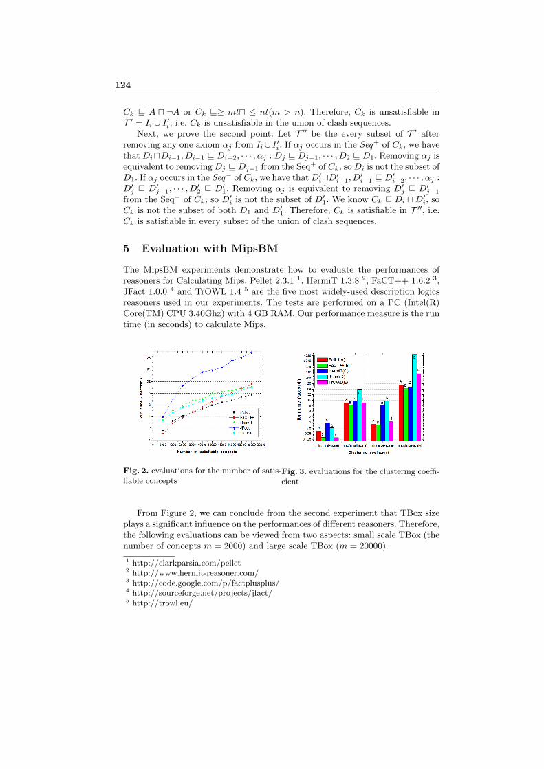
Ck v A u ¬A or Ck v≥ mtu ≤ nt(m > n). Therefore, Ck is unsatisfiable inT ′ = Ii ∪ I ′i, i.e. Ck is unsatisfiable in the union of clash sequences.

Next, we prove the second point. Let T ′′ be the every subset of T ′ afterremoving any one axiom αj from Ii ∪ I ′i. If αj occurs in the Seq+ of Ck, we havethat DiuDi−1, Di−1 v Di−2, · · · , αj : Dj v Dj−1, · · · , D2 v D1. Removing αj isequivalent to removing Dj v Dj−1 from the Seq+ of Ck, so Di is not the subset ofD1. If αj occurs in the Seq− of Ck, we have that D′iuD′i−1, D′i−1 v D′i−2, · · · , αj :D′j v D′j−1, · · · , D′2 v D′1. Removing αj is equivalent to removing D′j v D′j−1from the Seq− of Ck, so D′i is not the subset of D′1. We know Ck v Di uD′i, soCk is not the subset of both D1 and D′1. Therefore, Ck is satisfiable in T ′′, i.e.Ck is satisfiable in every subset of the union of clash sequences.

5 Evaluation with MipsBM

The MipsBM experiments demonstrate how to evaluate the performances ofreasoners for Calculating Mips. Pellet 2.3.1 1, HermiT 1.3.8 2, FaCT++ 1.6.2 3,JFact 1.0.0 4 and TrOWL 1.4 5 are the five most widely-used description logicsreasoners used in our experiments. The tests are performed on a PC (Intel(R)Core(TM) CPU 3.40Ghz) with 4 GB RAM. Our performance measure is the runtime (in seconds) to calculate Mips.

Fig. 2. evaluations for the number of satis-fiable concepts

Fig. 3. evaluations for the clustering coeffi-cient

From Figure 2, we can conclude from the second experiment that TBox sizeplays a significant influence on the performances of different reasoners. Therefore,the following evaluations can be viewed from two aspects: small scale TBox (thenumber of concepts m = 2000) and large scale TBox (m = 20000).

1 http://clarkparsia.com/pellet2 http://www.hermit-reasoner.com/3 http://code.google.com/p/factplusplus/4 http://sourceforge.net/projects/jfact/5 http://trowl.eu/

124

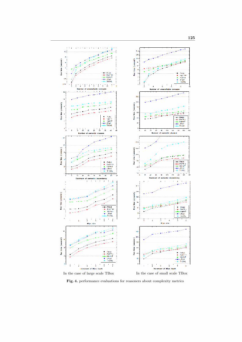
In the case of large scale TBox In the case of small scale TBox

Fig. 4. performance evaluations for reasoners about complexity metrics

125

After the evaluation experiments, we give a further analysis from two per-spectives.

What makes an incoherent TBox difficult to calculate Mips? In order toanswer this question, we consider the impact of construction parameters onstructure complexity of incoherent terminology. A large number of satisfiableconcepts mean a large size of TBox, Reasoners have to take a lot of time toperform satisfiability checking, so the run time becomes longer. There are manyrelevance relations between one concept and others if the concept depth is large,as the number of semantic clusters increases, the number of semantic dependen-cies between the concepts will grow significantly. The Mips size corresponds tothe scale of minimal conflict axiom set, our reasoners need to find the minimalconflict axiom set of the incoherent TBox, thus the size of semantic dependencyis strictly determined by the Mips depth. According to Definition 9, the clashsequences of unsatisfiable concepts correspond to the increase of Mips depth, thelarger the depth is, the longer the clash sequences are, therefore, a larger valueof the increase of Mips depth leads to a higher complex of incoherent TBox.

Which is the most appropriate reasoner to solve Mips problem? Because ofthe differences of optimization approaches, the five reasoners have different per-formances for the same benchmark test data. When the number reaches 8000,Pellet is faster than FaCT++, when reaches 14000, TrOWL is faster than FaC-T++, and when reaches 18000, HermiT performs better than FaCT++. In theprocess of consistency checking, HermiT uses the anywhere blocking techniqueto limit the sizes of models which are constructed, so it has an advantage overABox. Unfortunately, the ontology test data generated by our MipsBM only con-sists of TBox, thus the advantages haven’t been fully fulfilled. Our experimentsshow that timeout is the main reason to cause the failures of JFact, especiallyfor a large inputs, It is because JFact takes longer to load the TBox than others.In the case of large scale TBox, JFact fails to resolve the Mips problems whenthe number of clusters increases beyond 80 in the fourth experiment.

6 Conclusion and future work

This paper presents a benchmark to generate different complicated terminologiesto evaluate the performances of description logics reasoners for calculating Mips.Our purpose is to find out the reasons which result in the difficulty and high costof ontology debugging. Experiments show that the six construction parameterscan fully reflect the complexity of incoherent TBox.

As for future work, we plan to improve our benchmark under realistic se-mantic web conditions to evaluate reasoners by using realistic TBox data, andfocus on different ontology reasoning and debugging algorithms to evaluate theircompleteness and correctness by using our extended benchmark.

References

1. Sirin Evren, Parsia Bijan, et al., Pellet:A practical OWL-DL reasoner, Web Se-mantics: science, services and agents on the World Wide Web, 2007, 5(2):51-53.

126

2. Rob Shearer, Boris Motik, and Ian Horrocks, HermiT: A highly-efficient owl rea-soner, in: Proceedings of the 5th International Workshop on OWL: Experiencesand Directions. Karlsruhe, Germany. 2008.

3. Dmitry Tsarkov and Ian Horrocks, FaCT++ Description Logic Reasoner: SystemDescription, in: Proceddings of Third International Joint Conference on AutomatedReasoning. Seattle, WA, USA, 2006, pp.292-297.

4. Edward Thomas, Jeff Z. Pan, Yuan Ren, TrOWL: Tractable OWL 2 ReasoningInfrastructure, in: Proceedings of 7th Extended Semantic Web Conference. Herak-lion, Crete, Greece, 2010, pp.431-435.

5. Yuanbo Guo, Zhengxiang Pan, and Jeff Heflin, LUBM: A benchmark for OWLknowledge base systems, Web Semantics: Science, Services and Agents on theWorld Wide Web, 2005, 3(2): 158-182.

6. Li Ma, Yang Yang, Zhaoming Qiu, et al., Towards a complete owl ontology bench-mark, in: Proceedings of the 3rd European Semantic Web Conference (ESWC),Budva, Montenegro, June, 2006, pp.125-139.

7. Yingjie Li, Yang Yu and Jeff Hefli, A multi-ontology synthetic benchmark for thesemantic web, in: Proceedings of the 1st International Workshop on Evaluation ofSemantic Technologies, Shanghai, China. 2010.

8. Alfio Ferrara, Stefano Montanelli, et al., Benchmarking matching applications onthe semantic web, The Semanic Web: Research and Applications, Springer BerlinHeidelberg, 2011, pp.108-122.

9. Christian Meilicke, Raul Garca-Castro, et al., MultiFarm: A benchmark for mul-tilingual ontology matching, Web Semantics: Science, Services and Agents on theWorld Wide Web, 2012, 15: 62-68.

10. Maria Rosoiu, Cassia Trojahn Dos Santos, et al., Ontology matching benchmarks:generation and evaluation, in: Proceedings of the 6th ISWC workshop on ontologymatching (OM), 2011, pp.73-84.

11. Zhengxiang Pan, Benchmarking DL Reasoners Using Realistic Ontologies, in: Pro-ceedings of the OWLED05 Workshop on OWL: Experiences and Directions, Gal-way, Ireland, November, 2005, 188.

12. Tom Gardiner, Ian Horrocks and Dmitry Tsarkov, Automated benchmarking ofdescription logic reasoners, in: Proceedings of the 19th International Workshop onDescription Logics, Windermere, Lake District, UK, May, 2006, pp. 167-174.

13. Jurgen Bock, Peter Haase, et al., Benchmarking OWL reasoners, in: Proceedingsof the ARea 2008 Workshop, Tenerife, Spain, June, 2008.

14. Samantha Bail, Bijan Parsia, Ulrike Sattler, JustBench: a framework for OWLbenchmarking, in: Proceedings of the 9th International Semantic Web Conference(ISWC), Shanghai, China, November, 2010, pp.32-47.

15. Yong-Bin Kang, Yuan-Fang Li, Shonali Krishnaswamy, Predicting reasoning per-formance using ontology metrics, in: Proceedings of the 11th International Seman-tic Web Conference (ISWC), Boston, MA, USA, November, 2012, pp.198-214.

16. Ji Qiu, Gao Zhiqiang, Huang Zhisheng, et al., Measuring effectiveness of ontologydebugging systems, Knowledge-Based Systems, 2014, 71: 169-186.

17. Kathrin Dentler, Ronald Cornet, et al., Comparison of reasoners for large ontologiesin the OWL 2 EL profile, Semantic Web, 2011, 2(2): 71-87.

18. Stefan Schlobach, Zhisheng Huang, Ronald Cornet, et al., Debugging incoherentterminologies, Journal of Automated Reasoning, 2007, 39(3):317-349.

19. Aditya Kalyanpur, Debugging and repair of owl ontologies, Washington DC, Amer-ican: The University of Maryland, 2006.

127