Embed Size (px)
Citation preview
B U L L E T I N
SÉRIE:
RECHERCHES SUR LES DÉFORMATIONS
Comité de Rédaction de la Série
P. DOLBEAULT (Paris), H. GRAUERT (Göttingen),O. MARTIO (Helsinki), W.A. RODRIGUES, Jr. (Campinas, SP), B. SENDOV (Sofia),
C. SURRY (Font Romeu), P.M. TAMRAZOV (Kyiv), E. VESENTINI (Torino),L. WOJTCZAK (£ódŸ)
Volume LVII
Volume LVIII
£ÓD� 2008
JULIAN £AWRYNOWICZRédacteur en chef et de la Série:
N
DE LA SOCIÉTÉ DES SCIENCES
ET DES LETTRES DE £ÓD�
Secrétaire de la Série:JERZY RUTKOWSKI
������� ���� �� �������������� ��� � � �� ���������������� ��
�� � ���� � �� ��� !"# ���� � �� ��$%&�"' �("�)�*��+ �� � ���� � �� �,
��-"� + �). �)� �&�$
/(")� & $�-�*0" 1)")���0" ��)����%���" 2"��� � �&�� )�*��" /('�&�3�
�� 4��2 ����5 ,��
/(")�� ��2"��" ��� �3&�
���" ��-$���%��(+ 6�1" 7��"%*&(�
8%�� � �$%"�"+ ������� ��*���� 9: ��� � � ;"�"�" ��
�� � <�, �� �� �� ,9
INSTRUCTION AUX AUTEURS1. La presente Serie du Bulletin de la Societe des Sciences et des Lettres de �Lodzcomprend des communications du domaine des mathematiques, de la physiqueainsi que de leurs applications liees aux deformations au sense large.
2. Toute communications est presentee a la seance d’une Commission de la Societepar un des membres (avec deux opinions de specialistes designes par la Re-daction). Elle doit lui etre adressee directement par l’auteur.
3. L’article doit etre ecrit en anglais, francais, allemand ou russe et debute parun resume en anglais ou en langue de la communication presentee. Dans tousles travaux ecrits par des auteurs etrangers le titre et le resume en polonaisseront prepares par la redaction. Il faut fournir le texte original qui ne peutcontenir plus de 15 pages (plus 2 copies).
4. Comme des articles seront reproduits par un procede photographique, les au-teurs sont pries de les preparer avec soin. Le texte tape sur un ordinateur dela classe IBM PC avec l’utilisation d’une imprimante de laser, est absolumentindispensable. Il doit etre tape preferablement en AMS-TEX ou, exception-nellement, en Plain-TEX ou LATEX. Apres l’acceptation de texte les auteurssont pries d’envoyer les disquettes (PC). Quelle que soient les dimensions desfeuilles de papier utilisees, le texte ne doit pas depasser un cadre de frappe de12.3 × 18.7 cm (0.9 cm pour la page courante y compris). Les deux margesdoivent etre de la meme largeur.
5. Le nom de l’auteur (avec de prenom complet), ecrit en italique sera place a la1ere page, 5.6 cm au dessous du bord superieur du cadre de frappe; le titre del’acticle, en majuscules d’orateur 14 points, 7.1 cm au dessous de meme bord.
6. Le texte doit etre tape avec les caracteres Times 10 points typographiques etl’interligne de 14 points hors de formules longues. Les resumes, les renvois,la bibliographie et l’adresse de l’auteurs doivent etre tapes avec les petitescaracteres 8 points typographiques et l’interligne de 12 points. Ne laissez pasde ”blancs” inutiles pour respecter la densite du texte. En commencant letexte ou une formule par l’alinea il faut taper 6 mm ou 2 cm de la margegauche, respectivement.
7. Les texte des theoremes, propositions, lemmes et corollaires doivent etre ecritsen italique.
8. Les articles cites seront ranges dans l’ordre alphabetique et precedes de leursnumeros places entre crochets. Apres les references, l’auteur indiquera sonadress complete.
9. Envoi par la poste: protegez le manuscript a l’aide de cartons.10. Les auteurs recevront 20 tires a part a titre gratuit.
Adresse de la Redaction de la Serie:Departement d’Analyse complexe et Geometrie differentielle
de l’Institut de Mathematiques de l’Academie polonaise des SciencesBANACHA 22, PL-90-238 �LODZ, POLOGNE

Name and surname of the authors
TITLE – INSTRUCTION FOR AUTHORSSUBMITTING THE PAPERS FOR BULLETIN
Summary
Abstract should be written in clear and concise way, and should present all the main
points of the paper. In particular, new results obtained, new approaches or methods applied,
scientific significance of the paper and conclusions should be emphasized.
1. General information
The paper for BULLETIN DE LA SOCIETE DES SCIENCES ET DES LETTRESDE �LODZ should be written in LaTeX, preferably in LaTeX 2e, using the style (thefile bull.cls).
2. How to prepare a manuscript
To prepare the LaTeX 2e source file of your paper, copy the template file in-str.tex with Fig1.eps, give the title of the paper, the authors with their affilia-tions/addresses, and go on with the body of the paper using all other means andcommands of the standard class/style ‘bull.cls’.
2.1. Example of a figure
Figures (including graphs and images) should be carefully prepared and submittedin electronic form (as separate files) in Encapsulated PostScript (EPS) format.
Fig. 1: The figure caption is located below the figure itself; it is automatically centered andshould be typeset in small letters.
2.2. Example of a table
Tab. 1: The table caption is located above the table itself; it is automatically centered andshould be typeset in small letters.
Description 1 Description 2 Description 3 Description 4
Row 1, Col 1 Row 1, Col 2 Row 1, Col 3 Row 1, Col 4Row 2, Col 1 Row 2, Col 2 Row 2, Col 3 Row 2, Col 4
[4]

3. How to submit a manuscript
Manuscripts have to be submitted in electronic form, preferably via e-mail as at-tachment files sent to the address [email protected]. If a whole manuscriptexceeds 2 MB composed of more than one file, all parts of the manuscript, i.e.the text (including equations, tables, acknowledgements and references) and figures,should be ZIP-compressed to one file prior to transfer. If authors are unable to sendtheir manuscript electronically, it should be provided on a disk (DOS format floppyor CD-ROM), containing the text and all electronic figures, and may be sent byregular mail to the address: Department of Solid State Physics, University ofLodz, Bulletin de la Societe des Sciences et des Lettres de �Lodz, Pomorska149/153, 90-236 Lodz, Poland.
References
[1]
Affiliation/Address
[5]
TABLE DES MATIERES
1. C. Surry, On earth contact in plane elasticity with Coulombfriction. Variational elliptic inequalities – obstacle problem . . . 7–18
2. D. A. Mierzejewski, Investigation of quaternionic quadraticequations II. Method of solving an equation with left coefficients 19–24
3. H. Shimada, S. V. Sabau, and R. S. Ingarden, The (α, β)-metric for Finsler space and its role in thermodynamics . . . . . . . 25–38
4. H. Shimada, S. V. Sabau, and R. S. Ingarden, The Randersmetric and its role in electrodynamics . . . . . . . . . . . . . . . . . . . . . . . . 39–49
5. R. S. Ingarden and J. �Lawrynowicz, Finsler geometry andphysics. Mathematical overview . . . . . . . . . . . . . . . . . . . . . . . . . . . . . . 51–56
6. L. Wojtczak, Some remarks on GMR . . . . . . . . . . . . . . . . . . . . . . . . 57–61
7. J. Rutkowski and L. Wojtczak, Pressure dependence of melt-ing temperature . . . . . . . . . . . . . . . . . . . . . . . . . . . . . . . . . . . . . . . . . . . . . . 63–67
8. H. M. Polatoglou and V. Gountsidou, Mechanical propertiesof functional non-linear materials with nanostructure . . . . . . . . . 69–78
9. G. Moutsinas and H. M. Polatoglou, A dynamical approachto populations with inheritable characteristics . . . . . . . . . . . . . . . . 79–87
10. G. Karwasz, Experimental Modern Physics: why do we needNew Mathematics? . . . . . . . . . . . . . . . . . . . . . . . . . . . . . . . . . . . . . . . . . . . 89–96
PL ISSN 0459-6854
B U L L E T I NDE LA SOCIETE DES SCIENCES ET DES LETTRES DE �LODZ
2008 Vol. LVIII
Recherches sur les deformations Vol. LVII
pp. 7–18
Claude Surry
ON EARTH CONTACT IN PLANE ELASTICITYWITH COULOMB FRICTIONVARIATIONAL ELLIPTIC INEQUALITIES – OBSTACLE PROBLEM
Summary
This paper summarizes the research published in this journal in the years 2003–2008 inrelation with earth contact in plane elasticity with Coulomb friction from the point of viewof methods used: a discussion of some variational elliptic inequalities and solving certainobstacle problems.
1. Introduction
Let Ω be a bounded open set in Rn with a regular boundary Γ = δΩ. We considerin Ω the partial differential equation
Aϑ =n∑i=1
n∑j=1
∂
∂κi
(αij
∂ϑ
∂κj
)+
n∑i=1
αi(κ, ϑ)∂ϑ
∂κi+ α0(κ, ϑ)ϑ.(1)
The functions aij , ai, a0 satisfy a0, ai, aij ∈ L∞(Ω) with real values∑i,j
aijξiξj ≥ α∑i
ξ2i , α > 0,(2)
∑i,j
ai,jξiξj +∑
aiξiξ0 + a0ξ20 ≥ α
∑i
(ξ2i + ξ20
).(3)
A is an elliptic operator of second order which is not necessarily symmetric withcoefficients which may be discontinuous. We want to find a function u, which is real,defined on Ω, and satisfies:
8 C. Surry
⎧⎨⎩
Au − f ≤ 0,u− ψ ≤ 0,(Au − f)(u− ψ) ≡ 0 on Ω,
(4)
u = 0 on Γ = ∂Ω.(5)
There is a compatibility condition: if u is a “strong solution”, the conditions
u− ψ ≤ 0 in Ω,
u = 0 on ∂Ω = Γ
are compatible if and only if
ψ ≥ 0 on Γ.(6)
Consider the third condition (1–4); Ω is divided in two regions
Ω1 = {κ| u = ψ},Ω2 = {κ| u < ψ} = {κ| Au = f}(7)
on the interface S = ∂Ω1 ∩ ∂Ω2. If u is a regular solution, we have⎧⎨⎩
u= ψ,∂
∂nu=
∂
∂nΨ.
(8)
S is not known and it is a free boundary problem [2] (flow in porous medium undera dam). We can now precise the variational problem to be solved.
2. Variational inequality
2.1. Sobolev spaces [1, 6 I, 8]
Let D(Ω) to be space of functions which are infinitely differentiable with real valueson Ω ∈ C
∞(Ω), D′(Ω) – distribution space on Ω, LP (Ω) – the space of functionswith real values on Ω, u – a real function such that∫
Ω
uPdΩ < +∞
and L2(Ω) – a Hilbert space with the scalar product
(f · g) =∫Ω
gfdΩ.(9)
Next let
H1(Ω) ={v| v ∂v
∂κi∈ L2(Ω) (i = 1, n)
}.(10)
On earth contact in plane elasticity with Coulomb friction 9
H1(Ω) is a Sobolev space which is Hilbertian for the scalar product
(u, v)H1(Ω) = (u, v) +∫Ω
n∑i=1
∂u
∂κidΩ = (u, v) +
n∑i=1
(∂u
∂κi,∂v
∂κi
)dΩ.(11)
It is shown [1] that
H10 (Ω) = {v| v ∈ H1(Ω), v = 0 on Γ}.(12)
Here H10 (Ω) is the closure of D(Ω) in H1(Ω).
2.2. Bilinear form a(u, v)
For (u, v) ∈ H1(Ω) we consider
a(u, v) =∑i,j
∫Ω
aij∂u
∂κj
∂v
∂κidΩ +
∑i
∫Ω
ai(κ, u)∂u
∂κivdΩ +
∫Ω
a0uvdΩ;(13)
it is a continuous bilinear form on H1(Ω) ×H1(Ω).By duality, we identify L2(Ω) to its dual. The dual space of H1
0 (Ω) is identifiedto a subspace of D′(Ω) and to a on space of L2(Ω), it is denoted by H−1(Ω) and wehave:
H10 (Ω) ⊂ L2(Ω) ⊂ H−1(Ω).(14)
We verify that
v ∈ H1(Ω) ⇒ Av ∈ H−1(Ω),(15)
where A is a continuous linear operator from H1(Ω) onto H−1(Ω).If u ∈ H1(Ω) and
∀v ∈ H10 (Ω), (Au, v) = a(u, v),(16)
the relations (2) and (8) hold for any v ∈ D(Ω) and then, we pass to the limit.
H10 (Ω) is the closure of D(Ω) in H1(Ω).(17)
2.3. Variational inequality for 4) and 5) [6 II, 7, 9, 14 I]
Let K be a convex set:
K ={v| v ∈ H1
0 (Ω); v ≤ ψ on Ω}
;(18)
if u is a solution of (4), (5) with
u ∈ K,(19)
then (4) is equivalent to
(Au− f, w − u) ≥ 0.(20)
With the use of (16) and (20), we can see that
∀v ∈ K a(u, v − u) ≥ (f, v − u).(21)
10 C. Surry
Precisely, we want to find u ∈ K such that ∀v ∈ K the condition (21) holds. Wehave a variational inequality with:
– a Hilbert space (we put H10 (Ω) = V );
– a closed convex set K �= ∅;– a bilinear form a(u, v) continuous on V × V ;– a linear form (f, v) continuous on V .
We can now ask the question: Is the problem (21) well posed?The solution of the problem is regular and monotoneous.If in (18), we take ψ = +∞
K = H10 (Ω)(22)
and
∀v ∈ H10 (Ω) a(u, v) = (f, v)(23)
or
{Au = f in Ω|u = 0 on Γ} ,(24)
then we have a Dirichlet Problem.
2.4. Uniqueness [4]
Theorem 1. We suppose the relations (2), (3), f ∈ L2(Ω), and ψ ∈ H1(Ω) withψ ≥ 0 on Γ. Then the problem (21) has a unique solution.
If u1 and u2 are two possible solutions, take u = u1 in Ω and u = u2 in Ω (23).Then we get
a(u1, u1 − u2) ≥ (f, u1 − u2),
a(u2, u1 − u2) ≥ (f, u1 − u2)
and by substraction
a(u1 − u2, u1 − u2) ≤ 0.
By (3), we have
a(v, v) ≥ α‖v‖2,
‖v‖2 = (v, v)H1(Ω),
(25)
hence (21) implies
μ1 − u2 = 0 on Ω.
On earth contact in plane elasticity with Coulomb friction 11
3. Penalization [14 II]. Existence of a solution of (21)
We want to solve (21) and we choose a penalized method which is often used inconvex-numerical problems.
3.1. Penalized equation
If v ∈ H1(Ω), we define
v+ = sup(v, 0), v− = sup(−v, 0),
v = (v+ − v−).(26)
We have [1]:
v+ ∈ H1(Ω), v− ∈ H1(Ω),(27)
and ‖v+‖ ≤ ‖v‖ if v+, v− ∈ H1(Ω) ×H1(Ω). For any ε > 0, we define
Auε +1ε
(uε − ψ)+ = f on Ω,(28)
uε = 0 on Γ.(29)
Relations (28)–(29) give the penalized problem linked to (21). In this nonlinearproblem the goal is now to pass to the limit when ε→ 0.
Theorem 2. Relations (2)–(3) hold for f ∈ L2(Ω), ψ ∈ H1(Ω) and ψ ≥ 0 on Γ; thesystem (28)–(29) has a unique solution.
Proof. Define
β(v) =1ε
(v − ψ)+.(30)
Because monotonicity of the operator β(v) acting from H10 (Ω) onto L2(Ω), we have
(β(u) − β(v), u − v) ≥ 0;(31)
moreover β(v) maps H10 (Ω) in H1
0 (Ω). On the boundary, we have β(v) = 0 sinceψ ≥ 0 on Γ. The functions u1ε and u2ε form a solution of the it nonlinear problem(28)–(29); we have
A(u1ε − u2ε) + β(u1ε − β(u2ε) = 0.(32)
Take the scalar product with u1ε − u2ε; we get
a (μ1ε − u2ε, μ1ε − u2ε) + (β(μ1ε) − β(u2ε), u1ε − u2ε) = 0(33)
with (31). Hencea (μ1ε − u2ε, u1ε − u2ε) ≤ 0
andμ1ε = μ2ε on Ω.
12 C. Surry
Proof of existence [2]. By simplification, we set
με = ω
and we want to find ω ∈ H10 (Ω) such that:
Aω +1ε
(ω − ψ)+ = f.(34)
We define a family of spaces Vh (h→ 0) so that
• Vh is finite dimensional (V (h) → +∞ if h→ 0);
• ∀v ∈ H10 (Ω), it exists a sequence vh ∈ Vh such that
‖v − vh‖ → 0 if h→ 0;(35)
• it exists v0 such thatv0 ∈ Vh ∩K.
Such a family exists (finite element family). We consider the approximate problemof (28)–(29): find ωh ∈ vh such that ∀v ∈ vh
a(ωh, v) +1ε
[(ωh − ψ)+ , v
]= (f, v).(36)
We have an equivalent formulation: ∀v ∈ H10 (Ω)
a(ω, v) +1ε
[(ω − ψ)+v
]= (f, v).(37)
The object (36) is finite dimensional. As a system of equations, it has a uniquesolution: we use the fixed point theorem of Brouwer [1] and the a priori estimatewhich follows. We take v = ωh − v0 and get
a(ωh, ωh − v0) +1ε
[(ωh − ψ)+ , ωh − v0
]= (f, ωh − v0)+ .(38)
Yet, [(ωh − ψ)+, ωh − v0
]=[(ωh − ψ)+, ωh − ψ
]+[(ωh − ψ)+, ψ − v0
]for v0 ∈ K and ψ ≥ v0 with [
(ωh − ψ)+, ψ − v0] ≥ 0.
We have also
(v+, v) = (v+, v+) = |v+|2 =∫Ω
(v+)2dΩ
and
a(ωh, ωh − v0) +1ε|(ωh − ψ)+|2 ≤ (f, ωh − v0)(39)
or
a(ωh, ωh) +1ε|(ωh − ψ)+|2 ≤ (f, ωh − v0) + a(ωh, v0).

On earth contact in plane elasticity with Coulomb friction 13
On the other hand a(ωh, ωh) ≥ α‖ωh‖2V and we get ∃C independent of h and ε such
that
‖ωh‖ ≤ C,(40)
1ε|(ωh − ψ)+|2 ≤ C.(41)
Take h→ 0. We can see that
ωh → ω in H10 (Ω) weakly.(42)
(The injection of H10 (Ω) in L2(Ω) is compact). Besides,
ωh → ω in L2(Ω) strongly(43)
and(ωh − ψ)+ → (ω − ψ)+ in L2(Ω) strongly.
For any v ∈ H10 (Ω) = V , by (35) we can find a sequence vh ∈ Vh such that ‖v−vh‖ →
0 and we have
a(ωh, vh) +1ε
[(ωh − ψ)+, vh
]= (f, vh).(44)
Letting h→ 0, by (44) we get
a(ω, v) +1ε
[(ω − ψ)+, v
]= (f, v) ∀v ∈ H1
0 (Ω)
and ω = uε.The solution uε is unique. It is not necessary to take the extraction of a subse-
quence. This proof is constructive and we use the finite element method in (35). Wecan avoid the use of the compactness of the injection from H1
0 (Ω) into L2(Ω) if weuse the monotonicity of the operator β(v) (31).
3.2. Resolution of the variational inequality
Take ε→ 0; by (40) we have‖ωh‖ ≤ C
or
‖uε‖ ≤ C(45)
and1ε|(uε − Ψ)+|2 ≤ C.(46)
We can extract a subsequence, noted still με, so that⎧⎨⎩
uε → u in H10 (Ω) weakly,
uε → u in L2(Ω) strongly,(uε − ψ)+ → (u− ψ)+ in L2(Ω) strongly.
By (22) we have
(u− ψ)+ = 0(47)
14 C. Surry
and
u ∈ K.(48)
Then, by the uniqueness: u = u, verify that
a(u, v − u) ≥ (f, v − u) ∀v ∈ K.(49)
For v ∈ K we have β(v) = 0.Use (34) and form the scalar product by v − uε. We get
a(uε, v − uε) + [β(uε) − β(v), uε − v] = (f, v − uε)
or
a(uε, v − uε) − (f, v − uε) = [β(uε) − β(v), uε − v] ≥ 0
and
a(uε, v) − (f, v − uε) ≥ a(uε, uε)
Letting ε→ 0, we have
a(u, v) − (f, v − u) ≥ lim inf a(uε, uε) ≥ a(u, u)
and finally we obtain (49).
4. Regularity [14 II, 15, 16]
Theorem 3. We suppose (2)–(3), f ∈ L2(Ω),
ψ ∈ H1(Ω) with ψ ≥ 0 on Γ,
and
Aψ ∈ L2(Ω),(50)
then the solution of the variational inequality is such that
Au ∈ L2(Ω).(51)
Proof. Choose Au = f , where f ∈ L2(Ω) and u can be looked as a solution of theclassical problem {
Au = f on Ω,u = 0 on ∂Ω.
(52)
If Γ and the coefficients of A are enough regular we deduce:
μ ∈ H2(Ω).(53)
On earth contact in plane elasticity with Coulomb friction 15
Proof. We have (uε − ψ)+ ∈ H1(Ω) and
a[uε − ψ)+
]+
1ε|(uε − ψ)+|2 =
[f, (uε − ψ)+
],
(54)
a[(uε − ψ)+, (uε − ψ)+
]= a
[uε − ψ, (uε − ψ)+
].
Relations (54) can be written as:
a[(uε − ψ)+, (uε − ψ)+
]+
1ε|(uε − ψ)+|2 =
[f, (uε − ψ)+
]− a[ψ, (uε − ψ)+
](55)
=[f −Aψ, (uε − ψ)+
].
From (55) we deduce
1ε|(uε − ψ)+| ≤ |f −Aψ|.(56)
Yet,
Auε +1ε
(uε − ψ)+ = f
and
|Auε| ≤ f + |f −Aψ|.(57)
The function Auε is bounded in L2(Ω),
με → μ in H1(Ω) weakly,
andAu ∈ L2(Ω).
5. Monotonicity
We use the hypotheses of Theorem 3. The function μ(f, ψ) is an increasing functionof f and ψ with
f ≥ f, ψ ≥ ψ.(58)
Then we get following
Corollary. Under the above hypotheses
u(f , ψ) = u ≥ u(f, ψ) = u.(59)
Proof. We want to show that
(u− u)− = 0.(60)
16 C. Surry
We have
a(u, v − u) ≥ (f , v − u) ∀v ∈ K(ψ),(61)
a(u, v − u) ≥ (f, v − u) ∀v ∈ K(ψ).(62)
In (61) we take v equal to
(v − u) = (u− u)− or v = sup (u, u) ≤ ψ.
On the other hand, in (62) we take v equal to:
(v − u) = −(u− u)− or v = inf(u, u) ≤ ψ.
By addition we get
a[(u− u)−, (u− u)−
]= a
[u− u, (u− u)−
] ≤ 0
and, consequently, the inequality (59) u > u.We have defined a typical problem of variational inequality which can be deter-
mined by (21) and solved by the technique of semicontinuous nonlinear operatorswith a penalization method (37). For the proof we use a constructive method (finiteelement) which is a case of the Galerkin method [6 III, 14 I]. This problem is calledobstacle problem and can be extended to
Kψϑ =
{v ∈ H1
0 (Ω) | ϑ(κ) ≤ v(κ) ≤ ψ(κ) ∀κ ∈ Ω}.(63)
It exists a unique solution�u to ∀v ∈ Kψ
ϑ (κ) which is closed convex and
a
(�u, v − �
u
)≥(f, v − �
u
).(64)
The latter problem is the double obstacle problem. We have generalized the Lax-Milgram theorem [2] by using a theorem of fixed point [6, 14]. This typical problemuse the same procedure. Techniques as those of Touzaline [8] can now be applied,as we can see, to contact Coulomb problems, including friction, on elastic solids.Several papers in this direction have been published in the Bull. Soc. Sci. Lettres�Lodz Ser. Rech. Deform. [2, 3, 7, 9–13, 17]. This paper is a summary of a coursegiven in �Lodz by the author. Items [1, 4, 5] are the main references used.
References
[1] G. Duvant and J. L. Lions, Les inequations en mecanique et en physique, Ed. Dunod,Paris 1972.
[2] J. �Lawrynowicz, A. Mignot, L. C. Papaloucas, and C. Surry, Mixed formulation forelastic problems – existence, approximation, and application to Poisson structures,Banach Center Publications 37 (1996), 343–349.
[3] J. �Lawrynowicz and C. Surry, Semigroups vs. invariant sets and attractors, Bull. Soc.Sci. Lettres �Lodz 53 Ser. Rech. Deform. 42 (2003), 81–92.
[4] —, —, Attractors in the MINEA three-dimensional systems, ibid. 53 Ser. Rech.Deform. 42 (2003), 93–98.
On earth contact in plane elasticity with Coulomb friction 17
[5] A. L. Mignot, An enhanced assumed composite strain method in linear elasticity, ibid.56 Ser. Rech. Deform. 51 (2006), 49–81.
[6] — and C. Surry, Methodes d’elements finis mixtes pour les problemes d’elasticite I–III,ibid. 44 Ser. Rech. Deform. 17 (1994), 65–93, ibid. 45 Ser. Rech. Deform. 20 (1995),91–129, and ibid. 46 Ser. Rech. Deform. 21 (1996), 39–56.
[7] U. Perego, A variationally consistent generalized variable formulation for enhancedstrain finite elements, Comm. in Numer. Meth. in Eng. 16 (2000), 151–163.
[8] C. Surry, On qualitative analysis of dynamical systems, Bull. Soc. Sci. Lettres �Lodz53 Ser. Rech. Deform. 42 (2003), 45–55.
[9] —, Variational methods and some remarks concerning elasticity, ibid. 56 Ser. Rech.Deform. 50 (2006), 47–51.
[10] —, L. Wojtczak, J. Rutkowski, and Ilona Zasada, Applications of the finite elementsmethod to thin films description. A basic formulation, ibid. 55 Ser. Rech. Deform.46 (2005), 9–19.
[11] —, J. Rutkowski, L. Wojtczak, and Ilona Zasada, Small perturbations of thermo-elasto-plasticity in mechanics of continua. The use of finite elements method, ibid.55 Ser. Rech. Deform. 46 (2005), 165–183.
[12] A. Touzaline, A quasistatic unilateral contact problem with a solution-dependent co-efficient of friction for elastic materials, ibid. 57 Ser. Rech. Deform. 53 (2007), 7–22.
[13] —. Analysis and numerical approximation of an elastic frictionless unilateral contactproblem with normal compliance, ibid. 58 Ser. Rech. Deform. 55 (2008), 35–47.
[14] —, Analysis of a frictional contact problem with adhesion for nonlinear elastic ma-terials I. Problem formulation, existence and uniqueness; II. The penalized and reg-ularized problem, ibid. 58 Ser. Rech. Deform. 58 (2008), 61–74 and 75–82.
[15] — and A. L. Mignot, A quasistatic problem with unilateral contact and time-dependentTresca friction law for nonlinear elastic materials, ibid. 54 Ser. Rech. Deform. 44(2004), 45–59.
[16] —, —, A quasistatic contact problem with normal compliance and friction for non-linear elastic materials, ibid. 56 Ser. Rech. Deform. 49 (2006), 79–95.
[17] L. Wojtczak, J. Rutkowski, Ilona Zasada, and C. Surry, Applications of the finite ele-ments method to thin films description. Some comments, ibid. 55 (2005) Ser. Rech.Deform. 46 (2005), 185–202.
Laboratoire Felix Trombe
Institut de Sciences et de Genie
de Materiaux et Procedes
Centre National de la Recherche Scientifique
B.P. 5 Odeillo
F–66 125 Font Romeu Cedex
France
Presented by Claude Surry and Leszek Wojtczak at the Session of the Mathematical-Physical Commission of the �Lodz Society of Sciences and Arts on December 10, 2008

18 C. Surry
O KONTAKCIE Z POD�LOZEMW P�LASKICH ZAGADNIENIACH SPREZYSTOSCIZ UWZGLEDNIENIEM TARCIA KULOMBOWSKIEGOELIPTYCZNE NIEROWNOSCI WARIACYJNE – ZAGADNIENIE Z PRZESZKODAMI
S t r e s z c z e n i ePraca podsumowuje badania opublikowane w tym czasopismie w latach 2001–2008,
dotyczace kontaktu z pod�lozem w p�laskich zagadnieniach teorii sprezystosci z uwzglednie-niem tarcia kulombowskiego z punktu widzenia uzytych metod: rozwazania pewnych elip-tycznych nierownosci wariacyjnych i rozwiazywania pewnych zagadnien z przeszkodami.

PL ISSN 0459-6854
B U L L E T I NDE LA SOCIETE DES SCIENCES ET DES LETTRES DE �LODZ
2008 Vol. LVIII
Recherches sur les deformations Vol. LVII
pp. 19–24
Dmytro Mierzejewski
INVESTIGATION OF QUATERNIONIC QUADRATICEQUATIONS IIMETHOD OF SOLVING AN EQUATION WITH LEFT COEFFICIENTS
Summary
We have described a precise algorithm to solve any quaternionic equation of the formx2 + ax + b = 0, improving the procedure from [3]. It is a continuation of [1].
5. Notation and convention
This short contribution is one step more in investigation of solutions of quaternionicpolynomial equations. Previous works on this topic are, for example, [3], [4], [5], [2],[1].
We use standard notation i, j, k for the quaternionic imaginary units; recall that
i2 = j2 = k2 = −1, ij = −ji = k, jk = −kj = i, ki = −ik = j.
We always use natural subindices to denote the components of a quaternion:
x = x0 + x1i+ x2j + x3k, where x0, x1, x2, x3 ∈ R;
moreover here
the number x0 is called the scalar part of x;
x1i+ x2j + x3k is called the vector part of x;√x2
0 + x21 + x2
2 + x23 is called the modulus of x.
Note also that we deal with only real quaternions, i.e., their components are real;we use the word “quaternion” only for the real one and denote the system of all(real) quaternions by H.

20 D. Mierzejewski
6. Equations with left coefficients
In this paper only equations with left coefficients are investigated, that is,n∑�=0
a(�)x� = 0,(18)
where x is the unknown, a(0), . . . , a(n) are given quaternions. The work [3] contains atheory of how to solve any such equation. Our aim is to improve this theory makingit somewhat more applicable for solving given equations. We restrict our task byonly quadratic ones, that is,
a(2)x2 + a(1)x+ a(0) = 0,
where a(2) �= 0, or, after a simple transformation,
x2 + ax+ b = 0.(19)
The authors of [3] describe a simple method to find the scalar part and themodulus of the vector part of every solution of any equation of the form (18). As aresult one knows spheres containing solutions. Sometimes every point of such sphereis a solution (then this sphere is called a spherical solution), sometimes such spherecontains only one solution; other situations (for example, exactly two solutions onthe sphere) are impossible.
Yet, in [3] there is no explanation of how to guess which point of the sphere isa solution. Of course, it is simple in the case of a spherical solution: substitutingtwo different points from the sphere one sees that the both are solutions and makesthe conclusion that every point from this sphere is a solution. But in the case of aunique solution on the sphere it may be not so easy to guess which point should bechecked. The aim of this paper is to give a method to find this point.
7. The method
Let a quaternionic equation of the form (19) be given, where x is the unknown, aand b are given quaternions.
Note first of all that if a, b ∈ R then it is very simple to find all quaternionicsolutions of (19). Namely, if a2 − 4b ≥ 0 then the set of all real solutions of (19) issimultaneously the set of all its quaternionic solutions; if a2−4b < 0 then (19) hasa spherical solution (only one sphere), where the sphere has the centre α ∈ R andthe radius β > 0, where α + βi and α − βi are complex solutions of (19). Thesefacts can be easily implied by information from [3] and were explained also in [2].
Moreover it is useful to remember that, according to Theorem 3 from [2], a spher-ical solution can appear only if a, b ∈ R. So, now we can restrict our investigation byonly the case, where a or b is not real, and moreover we know that there is no spheri-cal solution in this case. According to [3], now the number of all solutions equals twoor one. We will not repeat here the corresponding theory, but the work [3] explains
Investigation of quaternionic quadratic equations II 21
how to understand how many solutions has the equation and how to calculate thescalar part and the modulus of the vector part of each solution.
So, let α be the scalar part of a solution of (19) (where a �∈ R or b �∈ R) and β
be the modulus of the vector part of this solution. By other words, denoting thissolution by α+ ξi+ ηj + ζk (where α, ξ, η, ζ ∈ R) we have:
ξ2 + η2 + ζ2 = β2.(20)
Our aim is to calculate ξ, η, and ζ. Note also that the solution being to be found isunique (for another solution another pair of α and β arises).
Let us apply a direct method applied also, for example, in [5], [1]. For this aimrewrite (19) decomposing every quaternion by the standard basis of H and substi-tuting the unknown solution instead of x:
(α+ξi+ηj+ζk)2+(a0+a1i+a2j+a3k)(α+ξi+ηj+ζk)+(b0+b1i+b2j+b3k) = 0.
Opening all brackets and then moving each imaginary unit out of new brackets,we pass to the following equation:
(α2 − ξ2 − η2 − ζ2 + a0α− a1ξ − a2η − a3ζ + b0) +
(2αξ + a0ξ + a1α+ a2ζ − a3η + b1)i+
(2αη + a0η − a1ζ + a2α+ a3ξ + b2)j +
(2αζ + a0ζ + a1η − a2ξ + a3α+ b3)k = 0.
Obviously, this equation is equivalent to the following system of four real equations:⎧⎪⎪⎨⎪⎪⎩
α2 − ξ2 − η2 − ζ2 + a0α− a1ξ − a2η − a3ζ + b0 = 0,2αξ + a0ξ + a1α+ a2ζ − a3η + b1 = 0,2αη + a0η − a1ζ + a2α+ a3ξ + b2 = 0,2αζ + a0ζ + a1η − a2ξ + a3α+ b3 = 0.
(21)
The last three equations of (21) constitute a system of linear equations:⎧⎨⎩
(2α+ a0)ξ − a3η + a2ζ = −a1α− b1,
a3ξ + (2α+ a0)η − a1ζ = −a2α− b2,
−a2ξ + a1η + (2α+ a0)ζ = −a3α− b3.
(22)
This system has three equations and three unknowns. Therefore, as a rule, it shouldhave a unique solution. So, if one solves the system (22) and the solution is uniquethen the problem is solved. But it is necessary to analyse also cases where the system(22) has another number of solutions.
Note first of all that the system (22) is always solvable. Really, if it were un-solvable then (19) would not have any solution of the form α + ξi + ηj + ζk, butthis is impossible if α is calculated correctly (according to [3]). So, it remains forus to analyse the case where (22) has infinitely many solutions. More exactly, threepossibilities remain: where the subspace of the solutions is one-dimensional (a line),where it is two-dimensional (a plane), and where it is three-dimensional (that is,every triplet of real numbers is a solution of (22)).
22 D. Mierzejewski
The case of the three-dimensional space of the solutions would be possible onlyif all coefficients of (22) equaled zero. Then we would have:
a1 = a2 = a3 = 0
and also−a1α− b1 = −a2α− b2 = −a3α− b3 = 0;
thusb1 = b2 = b3 = 0.
The equalitiesa1 = a2 = a3 = b1 = b2 = b3 = 0
mean that a, b ∈ R, but we have agreed to omit this case. So, the case of thethree-dimensional space is now impossible.
Then suppose that we have the case of a two-dimensional space of the solutions.Then the rank of the matrix of the system (22) equals 1. Write down this matrix:⎛
⎝ 2α+ a0 −a3 a2
a3 2α+ a0 −a1
−a2 a1 2α+ a0
⎞⎠ .(23)
Since the rank of the matrix (23) equals 1, any its two rows are proportional. Inparticular, looking at the second and third elements of the second and third rows,we can conclude that
2α+ a0
a1= − a1
2α+ a0.(24)
Such equality is impossible. Really, denoting the left-hand side by τ , we obtain
τ = −1τ
or τ2 = −1,
but here only real numbers are involved. Yet, it is necessary also to take into accountthat (24) can be true not necessarily in the precise sense: it is also possible that2α + a0 = a1 = 0. Considering analogously other lines of (23) we get that alsoa2 = a3 = 0. But then every element of the matrix equals 0, and thus its rank is 0,not 1. So, this case of a two-dimensional space of the solutions is impossible.
It remains to consider the case of a one-dimensional space of the solutions. In thiscase solving (22) one obtains expressions for two unknowns by one other unknown,for example:
η = λξ + μ, ζ = νξ + ρ,(25)
where λ, μ, ν, ρ are known real numbers. Then it is convenient to use (20). Substi-tuting (25) into (20) one gets:
ξ2 + (λξ + μ)2 + (νξ + ρ)2 = β2,
or
(1 + λ2 + μ2)ξ2 + 2(λμ+ νρ)ξ + (μ2 + ρ2 − β2) = 0.(26)
Investigation of quaternionic quadratic equations II 23
which is a quadratic equation with respect to ξ. Solving it one obtains at most twopossible values of ξ and thus (by (25)) at most two triplets of possible values of ξ,η, ζ. Then it is not difficult to check which from this two triplets represents thesolution of (19). By the way, for this aim it is enough to substitute these values ofξ, η, ζ to the first equation of the system (21). Note also that if the free unknownis not ξ (as in (25)) but η or ζ, then the situation is quite analogous since (20) issymmetric with respect to ξ, η, ζ.
As a conclusion from the considerations above we can formulate the followingproposition:
Proposition 6. Let a quaternionic equation of the form (19) be given, where x isthe unknown, a and b are given quaternions, and at least one from the quaternionsa and b is not a real number. Then in order to solve this equation it is sufficient tofulfil the following algorithm:
1. Find the scalar part and the modulus of the vector part of each solution of (19)by the method described in [3] (this method is also explained in [2]).
2. Take the scalar part α and the modulus β of the vector part of any one solutionof (19) and construct by them a system (22).
3. Solve the system (22). If its solution is unique then
x = α+ ξi+ ηj + ζk(27)
is a solution of (19) and proceed to item 6.
4. If (22) has infinitely many solutions then substitute the general solution of (22)to (20), solve the obtained quadratic equation, and calculate by its solutions allthe real unknowns. If the quadratic equation has a unique solution then (27) isa solution of (19) and proceed to item 6.
5. If the quadratic equation has two solutions then check which of them satisfiesthe first equation in (21). Chose the satisfying values of ξ, η, ζ, and (27) is asolution of (19).
6. If another solution of (19) remains to be calculated, then fulfil items 2–5 forits scalar part and the modulus of its vector part. Otherwise that is all.
Acknowledgment
This research was partially supported by State Foundation of Fundamental Re-searches of Ukraine (project no. 25.1/084).
References
[1] D. Mierzejewski, Investigation of quaternionic quadratic equations I. Factorizationand passing to a system of real equations, Bull. Soc. Sci. Lettres �Lodz 58 Ser. Rech.Deform. 56 (2008), 17–26.
24 D. Mierzejewski
[2] D. Mierzejewski, V. Szpakowski, On solutions of some types of quaternionic quadraticequations, ibid. Ser. Rech. Deform. 55 (2008), 49–58.
[3] A. Pogorui, M. Shapiro, On the structure of the set of the zeros of quaternionicpolynomials, Complex Variables and Elliptic Equations 49, no. 6 (2004), 379–389.
[4] V. Szpakowski, Solution of some quadratic equations of quaternionic variable, Sci-entific quest of young researchers. Edition II: collection of scientific works (inUkrainian), Zhytomyr State University, Ukraine, 2005, pp. 71–74.
[5] V. Szpakowski, Solution of general linear quaternionic equations, The XI KravchukInternational Scientific Conference (in Ukrainian), Kyiv (Kiev), Ukraine, 2006 p. 661.
Address until August 2008:
Department of Mathematical Analysis
Zhytomyr State University
Velyka Berdychivska Street 40
Zhytomyr, 10008
Ukraine
Address since September 2008:
Department of Economic Cybernetics and Information Technologies
Zhytomyr Branch of the European University
Prospekt Myru 59, Zhytomyr, 10004
Ukraine
E-mail: [email protected]
Presented by Andrzej �Luczak at the Session of the Mathematical-Physical Commis-sion of the �Lodz Society of Sciences and Arts on October 29, 2008
BADANIE KWADRATOWYCH ROWNANKWATERNIONOWYCH IIMETODA ROZWIAZYWANIA ROWNANIA O WSPO�LCZYNNIKACH LEWYCH
S t r e s z c z e n i eOpisujemy scis�ly algorytm rozwiazywania dowolnego rownania kwaternionowego postaci
x2 + ax + b = 0, udoskonalajac procedure z pracy [3]. Jest to kontynuacja pracy [1].
PL ISSN 0459-6854
B U L L E T I NDE LA SOCIETE DES SCIENCES ET DES LETTRES DE �LODZ
2008 Vol. LVIII
Recherches sur les deformations Vol. LVII
pp. 25–38
Hideo Shimada, Sorin Vasile Sabau, and Roman Stanis�law Ingarden
THE (α, β)-METRIC FOR FINSLER SPACE AND ITS ROLEIN THERMODYNAMICS
Summary
After recalling as examples the Randers and Matsumoto spaces, a presentation of gen-eralized Matsumoto spaces, introduced by the third author is given. The latter spacesappear to be of basic importance in thermodynamics, especially if the electrodynamicaleffects are also taken into account. Then, having in mind the applications mentioned, thebasic properties of (α, β)-metrics are discussed, spray and curvatures of Finsler spaces with(α, β)-metrics, volume forms in Finsler spaces with (α, β)-metric, and Finsler spaces with(α, β)-metric of Landsberg and Berwald type.
Introduction
Genealized Matsumoto spaces show the importance of Finsler spaces of (α, β)-metric,more general than the Randers spaces, in thermodynamics, especially when theelectrodynamical effects are also taken into account.
The importance of spray and curvatures of Finsler spaces with (α, β)-metrics areindicated and discussed as well as the Finsler spaces with (α, β)-metric of Landsbergand Berwald types.
1. The (α, β)-metrics. Definitions and examples
Example 1. Randers spaces. Taking into consideration applications of differential ge-ometry to the physical space-time, G. Randers remarked that the property of perfectsymmetry between opposite directions for any coordinate interval of a Riemannianspace might not be a suitable one. He points out in [R1941] that the most charac-teristic property of the physical world is the unidirection of time-like intervals, in
26 H. Shimada, S. V. Sabau, and R. S. Ingarden
other words, a metric with asymmetric properties is desirable (see in [AIM1993] or[M2003] and [vN1927]).
From a geometrical point of view it means that a metric F whose unit spherebundle, or indicatrix,
Ix := {y ∈ TxM : F (x, y) = 1},i.e. the locus of the end points of all unit lengths radiating from a certain point x iscentral symmetric, it is not suitable to applications to the physical space-time. Thisis the case of Euclidean and Riemannian metrics.
A natural way of introducing an asymmetry for a quadratic indicatrix is to dis-place the center of symmetry of the indicatrix. This observation leads to the so calledRanders metric
F (x, y) = α(x, y) + β(x, y)(1.1)
whereα(x, y) :=
√aij(x)yiyj
is a Riemannian metric on M , and β(x, y) := bi(x)yi is a linear 1-form.The condition for the displaced indicatrix to be a close, convex hypersurface
including the origin is
b :=√a(b, b) =
√aij(x)bibj ,
where (aij(x)) is the inverse matrix of (aij(x)).Remarkably, Randers spaces appear as the solution of Zermelo’s problem
[BRS2004] posed initially by Zermelo and generalized by Z. Shen. Namely, considera ship sailing on the open sea in calm waters. If a mild breeze comes up, how shouldthe ship be steered in order to reach a given destination in the shortest time possible?
Zermelo assumed that the open see is the Euclidean plane R2, but Z. Shen gener-alized the problem to the setting where the sea is a Riemannian manifold. An evenmore general case is when the sea is a Finslerian manifold, but we are not going todiscuss here this case.
Geometrically, the wind is represented by a vector field, say W , globally definedon the Riemannian manifold M . Firstly remark that the action of the wind is equiv-alent to a rigid translation of the Riemannian indicatrix. However, pay attention tothe fact that in order to keep a translated quadratic indicatrix, the wind has to bea mild breeze, i.e. the Riemannian length of the vector field W has to be less thanone.
An algebraic computation shows that the metric that minimizes the travel timeon the Riemannian manifold in the presence of the mild breeze is a Randers, i.e. aFinsler metric on the form (1.1). The paths of shortest time are the geodesics of thisRiemannian metric.
Remark that this metric cannot be a Riemannian one because the translatedindicatrix is not central symmetric, in other words is not quadratic in y anymore.Other details are given in the next chapter.
The (α, β)-metric for Finsler space and its role in thermodynamics 27
Example 2. Matsumoto spaces. One can show that if a person walks on a plane withan angle ε of inclination in a direction θ with constant speed v(:= a), then thedistance walked in the time t = 1 is
r = a+ w cos θ,(1.2)
wherew :=
g
2sin ε,
g is the gravitational constant, and (r, θ) are the polar coordinates in plane (see[AIM1993] for example.)
Equation (1.2) is the equation of a limacon, and by an old result of Pascal, it isknown that the limacon is convex if and only if a ≥ 2w.
Consider now a surface S ↪→ R3 embedded in the Euclidean space R3, given by
(x, y) ∈ S �→ (x, y, z = f(x, y)) ∈ R3.
The induced Riemannian metric on the surface S is given by
(aij) =(
1 + (fx)2 fxfyfxfy 1 + (fy)2
),
where fx and fy means partial derivative with respect to x and y, respectively.If we consider now a coordinate system (x, y, u, v) ∈ TM in the tangent bundle
of M , then the limacon equation (1.2) becomes
u2 + v2 + β2 = a√u2 + v2 + β2 − wβ,(1.3)
where we have put
β = fxu+ fyv = df, w =g
2.
Since the left hand side of (1.3) is exactly the induced Riemannian metric, wefurther put
α2 = aα− wβ.
In other words,
α2 = u2 + v2 + (fxu+ fyv)2
= (1 + f2x)u2 + 2fxfyuv + (1 + f2
y )v2.
Using now the Okubo method, namely “If h(v) = 0 is the indicatrix of a Minkow-ski space V n, where h := F − 1, then the fundamental function F is derived fromh(v/F ) = 0.”, from (1.3) one obtains
F =α2
aα− wβ.
By normalization, it results
F =α2
α− β.(1.4)
This is the so-called Matsumoto metric [M1989a, AIM1993, M2003].
28 H. Shimada, S. V. Sabau, and R. S. Ingarden
We remark that the convexity condition of the limacon implies that the Mat-sumoto metric (1.4) is a Finsler metric if and only if
f2x + f2
y ≤ 13.
Example 3. Generalized Matsumoto spaces. We can write the formula (1.4) as
F = β + α+β2
α− β
and then generalize it by taking the fundamental function
F = ε1α1 + ε2α2 + ε3α3 + . . .+ εnαn, n finite or not,(1.5)
with
α1 = bi(x)yi, α2 =√aij(x)yiyj, α3 = 3
√aijk(x)yiyjyk, . . . ,(1.6)
where
εl = εl(x), respectively: aij = aij(x), aijk = aijk(x), . . .(1.7)
are real-valued and continuous, respectively: positive-valued and continuous. Forfixed x these functions are considered as material constants describing thermody-namical properties of solid state, including the electromagnetic field and gravitation.
In this case the extended energy conservation law of electrodynamics, includingthe thermodynamical effects or – equivalently – the first principle of thermodynamicsincluding the electromagnetic effects, reads (in standard notation) [�L1986, �L2005,�LRW2003]:
12∂
∂t(D · E + B · H) + j · E + ∇(E × H) − 1
8π2
∂Aα∂t
(�Aσ +
∂2Aσ∂σ2
)= 0.(1.8)
The conservation law (1.8) corresponds to the five-dimensional space-time Lagran-gian
12(ε0εE
2 + μ−10 μ−1B2
)+
12ρ(v2 + v2
σ
)+ ρ (A · v + ηAσ − φ) ,(1.9)
η = 1 or − 1,
where σ stays for the stochastic variable representing entropy – the space-time ele-ment reads
ds2 = c2dt2 − dx21 − dx2
2 − dx23 − c2σdσ
2(1.10)
with cσ being a nonnegative constant.In (1.8) the first three terms correspond to the work of potential forces (in this
case of the electromagnetic nature), while the latter term represents the entropycontribution which measures the heat TS of the system. In order to interpret theentropy term appearing in the conservation law (1.8) we observe that the stochasticpotential ηAσ behaves analogously to the electromagnetic (space-time) potential(A, ϕ), i.e., it satisfies the equation
The (α, β)-metric for Finsler space and its role in thermodynamics 29
�Aσ +(∂2
∂σ2
)Aσ = vσ,(1.11)
where vσ plays the role of heat flow in the stochastic heat bath.Now we take into account the equation of motion for the stochastic variable σ:
we can see that the force acting in the case is of stochastic nature only. It can bereduced to (∂/∂t)Aσ:
d
dt
{mvσ
/[1 −
(1cv
)2
− η(cσc2vσ
)2]}
− ηecσc2
∂
∂tAσ.
Multiplying the both sides by vσ we get
(d/dt)(TS) = (e/c)vσ(d/dt)Aσ
and hence, for the temperature constant in time, we obtain the entropy productionequation
T (d/dt)S = (e/c)vσ(∂/∂t)Aσ,(1.12)
where the source of entropy can be related to the product of the heat flow, propor-tional to vσ in a natural way and the Onsager coefficient related to the stochasticalpotential ηAσ . Since
(∂/∂t)Aσ = (d/dt)(mvσ),
we obtain that
TS =14mv2
σ
and thus the heat is determined by the kinetic energy of the stochastic movement.
Generalizing now the examples above, one may define the notion of Finsler spacewith (α, β)-metric as follows.
The fundamental function F of a Finsler space Fn = (M,F ) is called an (α, β)-metric if F is an (1) p-homogeneous function of two arguments
α(x, y) :=√aij(x)yiyj , β(x, y) := bi(x)yi,
where α is a Riemannian metric on M , and β a differential 1-form. The space (M,a)is called the associated Riemannian space and bi the associated vector field.
A straightforward computation shows that the fundamental tensor g = (gij) ofan (α, β)-metric can be written in the form [M2003]:
gij = paij + p0bibj + p1(biYj + bjYi) + p2YiYj ,(1.13)
30 H. Shimada, S. V. Sabau, and R. S. Ingarden
where
p =1α
∂F
∂α, p0 =
∂2F
∂α2, p1 =
1α
∂2F
∂α∂β,
p2 =1α2
∂2F
∂α2− 1α3
∂F
∂α, Yi := airy
r.
(1.14)
In order to develop a consistent geometrical theory of Finsler spaces with (α, β)-metrics the strong convexity of the indicatrix is required, i.e. the condition that thefundamental tensor gij to be a positive definite matrix. This leads to a set of adifferential conditions on the fundamental metric gij .
A weaker condition would be the regularity of an (α, β)-metric, namelydet gij �= 0.
The following result is useful for giving the regularity conditions of an (α, β)-metric.
Lemma 1. [M2003]. Consider a regular n× n matrix A = (aij), and construct then × n matrix B = (bij), given by bij := aij + bicj, where b = (bi), c = (ci) aren-dimensional vectors.
If the quantity D := 1 + bicjaij does not vanishes, then B is a regular matrix,
and its inverse is given by
bij = aij − 1Dbicj , where bi = airbr and ci = cra
rj .
Using this lemma, the following holds.
Theorem 1. [AIM1993, M2003]. A Finsler space Fn = (M,F = α + β) with(α, β)-metric is regular if and only if the quantity
T = p(p+ p0b2 + p1β) + {p0p2 − (p1)2}γ2
=(Fα
)2 1β2
(∂F∂α
+ αγ2 ∂2F
∂α2
)(1.15)
does not vanish. Here γ2 := b2α2 + β2.
There is a lot a literature on the geometry of Finsler spaces with (α, β)-metric.See for example [M2003], [BCS2007]. Also, one can find in [SaS2001], [SaS2003]characterization of classes of (α, β)-metrics using the invariants (1.6).
Remark 1.1. The difficulties of computations in Finsler geometry is notorious. Finslerspaces with (α, β)-metrics make no exception.
We present here a technique of Shen (see [S2001]) to express geometrical objectsinitially depending on two variables, i.e. α and β, using a function ϕ of only onevariable.

The (α, β)-metric for Finsler space and its role in thermodynamics 31
Namely, for a fundamental function F = F (α, β) one can write
F = αϕ(s), s =α
β,(1.16)
where ϕ = ϕ(s) is a C∞ positive function defined on an open interval (−b0, b0).Using this notations, one can rewrite the fundamental tensor as
gij = ρaij + ρ0bibj + ρ1(biαj + bjαi) − sρ1αiαj ,
where
ρ = ϕ2 − sϕϕ′, ρ0 = ϕϕ′′ + (ϕ′)2,
ρ1 = −sρ0 + ϕϕ′, αi :=∂α
∂yi.
All the geometrical objects like connection coefficients, curvatures, etc., can nowbe expressed by means of ϕ = ϕ(s) and its derivatives. This notations may simplifythe computations in some cases.
Remark 1.2. Even after introducing the notation ϕ = ϕ(s), the computations, ofcurvature coefficients for example, are still hard.
A second remarkable simplification technique is the remark of Shen‘s (see[BCS2007]) that it is always possible to take a local coordinate system at x suchthat the Riemannian metric (aij) becomes Euclidean, i.e.
α2 =n∑i=1
(yi)2 and β = by1,
where b is a constant scalar.Here is a simple argument of this fact [K2006]. Let us denote by H the kernel of
β, i.e.
H := kerβ = {y ∈ TxM : β(y) = 0}.This is an (n − 1)-dimensional subspace of TxM , and let us denote by H⊥ the
orthogonal complement of H with respect to the Riemannian metric α. Remark thatH⊥ is an 1-dimensional subspace.
It follows that there exists an orthonormal basis e1, e2, . . . , en of TxM such thate1 ∈ H⊥, e2, . . . , en ∈ H and α(ei, ej) = δij .
In this case, an arbitrary vector y ∈ TxM can be written with respect to thebasis e1, e2, . . . , en as y = y1e1 + y2e2 + . . . ynen. It follows
α(y, y) =n∑i=1
(yi)2
and
β(y) = y1β(e1) + y2β(e2) + . . . ynβ(en) = y1β(e1) = by1.
32 H. Shimada, S. V. Sabau, and R. S. Ingarden
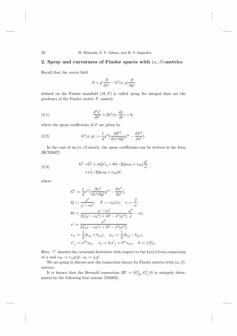
2. Spray and curvatures of Finsler spaces with (α, β)-metrics
Recall that the vector field
S = yi∂
∂xi−Gi(x, y)
∂
∂yi
defined on the Finsler manifold (M,F ) is called spray. Its integral lines are thegeodesics of the Finsler metric F , namely
d2xi
dt2+ 2Gi(x,
dx
dt) = 0,(2.1)
where the spray coefficients of F are given by
Gi(x, y) :=14gil( ∂F 2
∂xm∂ylym − ∂F 2
∂xl).(2.2)
In the case of an (α, β)-metric, the spray coefficients can be written in the form[BCS2007]:
Gi =Gi + αQsi0 + Θ(−2Qαs0 + r00
)yiα
+ψ(−2Qαs0 + r00
)bi,
(2.3)
where
Gi :=14ail( ∂α2
∂xm∂ylym − ∂α2
∂xl),
Q :=ϕ′
ϕ− sϕ′ , F := αϕ(s), s :=β
α,
Θ :=ϕ− sϕ′
2{(ϕ− sϕ′) + (b2 − s2)ϕ′′}ϕ′′
ϕ− sψ,
ψ :=ϕ′′
2{(ϕ− sϕ′) + (b2 − s2)ϕ′′} ,
rij :=12
(bi|j + bj|i), sij :=12
(bi|j − bj|i),
sij := aihshj , sj := bisij = bmsmj , b := ||β||a.
Here, “|” denotes the covariant derivative with respect to the Levi-Civita connectionof α and r00 := rijy
iyj, s0 := siyi.
We are going to discuss now the connection theory for Finsler metrics with (α, β)-metrics.
It is known that the Berwald connection BΓ = (Gijk, Gij , 0) is uniquely deter-
mined by the following four axioms [M2003]:

The (α, β)-metric for Finsler space and its role in thermodynamics 33
(1) F -metrical,
(2) Gijk = Gikj ,
(3)∂Gij∂yk
= Gijk,
(4) yrGirj = Gij .
(2.4)
The Berwald connection coefficients of an (α, β)-metric are given by
Gij = γi0j +Dij , Gijk = γijk +Di
jk,(2.5)
where
2Gi = γi00 + 2Di, Dij :=
∂Di
∂yj, Di
jk :=∂Di
j
∂yk,
γijk :=12air(
∂ajr∂xk
+∂akr∂xj
− ∂ajk∂xr
).
M. Matsumoto proved the following result [M2003].
Theorem 2. The Berwald connection BΓ = (Gijk, Gij , 0) of a Finsler space with
(α, β)-metric is given by (2.4), where the difference tensor Dij can be determined
from the relation
(F1Zr + αF2br)Dri = αF2br|iyr.(2.6)
Here,
Zi := airyr, F1 :=
∂F
∂α, F2 :=
∂F
∂β.
Indeed, since (2.5) satisfies the axioms (2)–(4) of (2.4), it is enough to verify if(1) is also satisfied. First, remark that
F;i :=∂F
∂xi−Gri
∂F
∂yr= F|i −Dr
iFr = 0, Fr :=∂F
∂yr,
where “;” and “|” denote the covariant derivative with respect to the Berwald con-nection BΓ and Riemannian Levi-Civita connection, respectively.
Next, remark that from
F|i = F1α|i + F2β|i = F2br|iyr,
Fr = F1αr + F2βr =F1Yrα
+ F2br, Yr = airyr,
it follows that F;i = 0 can be written in the form (2.6) and this proves the theorem.The locally Minkowski spaces with (α, β)-metric, generalized Berwald spaces
with (α, β)-metric, and Douglas spaces with (α, β)-metric are presented in the book[M2003].
Hilbert’s fourth problem is to characterize the metrics on an open domain in Rn
whose geodesics are straight lines. The Finsler metrics with this property are called
34 H. Shimada, S. V. Sabau, and R. S. Ingarden
projectively flat. It is know (see for example [M2003]) that a Finsler metric F isprojectively flat if and only if
∂2F
∂xk∂yiyk =
∂F
∂xi.(2.7)
On the other hand, recall the Beltrami theorem in Riemannian geometry, namelya Riemannian metric is projectively flat if and only if it is of constant sectionalcurvature.
If one investigate the same problem in Finsler geometry, the situation is quitedifferent than the Riemannian case. Namely, one can construct Finsler metrics whichare not of constant flag curvature, but projectively flat. See [MSY2006] for concreteexamples of projectively flat Finsler metrics of (α, β) type. More general results canbe found in [Br1997].
3. Volume forms in Finsler spaces with (α, β)-metric
Recall that the simplest volume form in Rn is the Euclidean volume form
dV := dx1 . . . dxn,(3.1)
where (xi) is a coordinate system on Rn.The Euclidean volume of a bounded open subset Ω ⊂ R
n is given by
V ol(Ω) :=∫
Ω
dV =∫
Ω
dx1 . . . dxn.(3.2)
More generally, it is well known that on a Riemannian manifold (M,a), theRiemannian metric a = (aij) determines the Riemannian canonical volume form
dVa :=√
det(aij)dx1 . . . dxn,(3.3)
and that the Riemannian volume of a bounded open subset Ω ⊂M is given by
Vol(Ω) :=∫
Ω
dVa =∫
Ω
√det(aij)dx1 . . . dxn.(3.4)
The generalization of these volume forms to the case of Finsler manifolds lead totwo canonical volume forms on a Finsler manifold, the Busemann-Hausdorff volumeform and the Holmes-Thompson volume form. Both of them reduce to the Rieman-nian canonical volume form in the case when the Finsler metric is Riemannian.
We are going to present these volume forms.
3.1. The Busemann-Hausdorff volume form
Let us denote by
Bn := {y = (yi) ∈ R
n : ||y|| < 1}(3.5)
the Euclidean ball in Rn and by
Bnx := {y = (yi) ∈ Rn : F (y) < 1}(3.6)
The (α, β)-metric for Finsler space and its role in thermodynamics 35
the Finslerian ball at x in Rn.The Finsler metric F determines the Busseman-Hausdorff volume form
dVBH := σF (x)dx1 . . . dxn,(3.7)
where
σF (x) :=Vol(Bn)Vol(Bnx )
.(3.8)
The Busseman-Hausdorff volume of a bounded subset Ω ⊂M is given by
VolBH(Ω) :=∫
Ω
dVBH =∫
Ω
σF (x)dx1 . . . dxn.(3.9)
Remark that σF (x) is actually the ratio of the Euclidean volume of the Euclideanball Bn ∈ Rn and the Euclidean volume of the Finslerian ball Bnx .
It was proved by H. Busemann that VolBH is the Hausdorff measure of theinduced Finslerian distance dF , provided F is reversible. Recall that reversible meansthat the Finsler metric is symmetric, i.e. F (−y) = F (y).
Recall that for any two points p, q ∈M , the Finslerian distance is defined by
dF (p, q) = infc
∫ 1
0
F (x,dx
dt)dt,
where the infimum is taken over all curves c : [0, 1] →M , c(0) = p, c(1) = q, joiningp and q.
3.2. The Holmes-Thompson volume
Recall that the Finsler fundamental function F induces the Riemannian metric
gij(y) := gij(x, y)dyi ⊗ dyj
in the tangent space TxM at each x ∈M .For the Finslerian ball Bnx one defines
σF (x) :=
∫Bn
xdet(gij)dy1 . . . dyn
Vol(Bn).(3.10)
Then, the n-form
dVHT := σF (x)dx1 . . . dxn,(3.11)
is called the Holmes-Thompson volume form on M .The Holmes-Thompson volume of a bounded subset Ω ⊂M is given by
VolHT (Ω) :=∫
Ω
dVHT =∫
Ω
σF (x)dx1 . . . dxn.(3.12)
As an immediate application of the above, one might try to compute the volumesfor (α, β)-metrics taking into account that on M there exists already the canonicalRiemannian volume form dVa.
36 H. Shimada, S. V. Sabau, and R. S. Ingarden
In [BCS2007] the authors perform this computation in the following way. For theFinsler space
Fn = (M,F = α+ β),
writeF = αϕ(s), s =
β
α.
Then, the Busemann-Hausdorff volume of F is given by
dVBH = f(b)dVa, f(b) :=
π∫0
sinn−2(t)dt/ π∫
0
sinn−2(t){ϕ(b cos t)}n dt,(3.13)
and the Holmes-Thompson volume is given by
dVHT = g(b)dVa, g(b) :=
π∫0
sinn−2(t)T (b cos(t))dt/ π∫
0
sinn−2(t)dt,(3.14)
where
T (s) = ϕ(ϕ− sϕ′)n−2{(ϕ− sϕ′) + (b2 − s2)ϕ′′}.(3.15)
Remark 3.1. For the particular case of a Randers space F = α+ β, we have
ϕ(s) = 1 + s, ϕ′(s) = 1, ϕ′′(s) = 0.
A straightforward computation shows that for a Randers metric the Holmes-Thompson volume and the associated Riemannian volume coincide, i.e. dVHT = dVa.
Remark 3.2. Let us consider again the case of a Randers space F = α + β. Then,one can show (see [S2001]) that
VolBH(M) =∫M
(1 − b2)n+1
2 dVa ≤ Vola(M).
4. Finsler spaces with (α, β)-metric of Landsbergand Berwald type
Recall that a Finsler space Fn = (M,F ) is said to be of Landsberg type if and only ifthe canonical parallel transport is a Riemannian canonical isometry. An equivalentdescription is through the Landsberg curvature tensor
Lijk = Aijk = −12Fls
∂3Gs
∂yi∂yj∂yk.(4.1)
Namely, a Finsler space whose Landsberg curvature L identically vanishes is ofLandsberg type.
On the other hand, a Finsler space whose canonical parallel transport is a linearisometry, or equivalently, whose Berwald curvature
P ij kl := −F ∂Γijk
∂yl(4.2)

The (α, β)-metric for Finsler space and its role in thermodynamics 37
vanishes, is called a Berwald space. This is equivalent with the fact that the Berwaldconnection coefficients Γijk are independent of y, or with the fact that the spraycoefficients Gs are quadratic in y.
From the definition it follows immediately that a Berwald metric is of Landsbergtype.
The converse is not true. However, the problem of finding an explicit example ofLandsberg metric that is not Berwald is an open problem in Finsler Geometry.
M. Matsumoto gave in [M1996] a list of rigidity conditions that almost suggestthat this kind of metrics does not exists. Here are few of them for the two-dimensionalcase.
Theorem 3. If a Randers surface is of Landsberg type, then it is Berwald.
Theorem 4. If a Kropina surface with b2 �= 0 is of Landsberg type, then it isBerwald.
Theorem 5. If a Matsumoto surface is of Landsberg type, then it is Berwald.
By analogy with those mythical single-horned horses whose power is exceededonly by their mystery, D. Bao called the Landsberg metrics that are not of Berwaldtype unicorns.
The first good news about the existence of unicorns came around 2002 fromR. L. Bryant who claimed in several occasions that despite Matsumoto’s rigidityresults, there is an abundance of such metrics in two dimensions.
A surprising news break out in 2006 when Asanov succeeded to construct y-localunicorns in dimension greater than two [A2006].
See an excellent discussion on the existence of unicorns by D. Bao in [B2007]. Weare going to describe Asanov’s unicorns using Bao’s notations.
Start with the product manifold
M = (0, 1) ×N,
where (N, h) is an arbitrary smooth (n− 1)-dimensional Riemannian manifold, andlet ϕ : (0, 1) → (0,∞) be any positive function that is not constant on (0, 1).
It is known that M can be endowed with the Riemannian warped product
a := dt× dt+ ϕ2(t)h
and the 1-form b := dt.Using these Asanov constructs an (α, β)-metric on M as follows. Put
q :=√α2 − β2
and
C1 : = any constant in the interval (−2, 2),
C2 : =
√1 − C2
1
4,
C3 : =C1/C2.
38 H. Shimada, S. V. Sabau, and R. S. Ingarden
Define the function
Φ :=
⎧⎪⎪⎪⎪⎪⎨⎪⎪⎪⎪⎪⎩
π
2+ arctan
(C3
2
)− arctan
(q + 1
2C1β
C2β
)if β ≥ 0,
−π2
+ arctan(C3
2
)− arctan
(q + 1
2C1β
C2β
)if β ≤ 0.
Then the (α, β)-metric
F = exp{C3
2Φ}√
β2 + C1βq + q2(4.3)
is an unicorn, provided n = dimM > 2.See also Shen’s discussion on the existence of (α, β) unicorns in arbitrary dimen-
sion [BCS2007].
References
[AIM1993–YS1977] See this issue, pp. 46-48.
Hideo Shimada and Sorin Vasile Sabau Roman Stanis�law Ingarden
Department of Mathematics Institute of Physics
Hokkaido Tokai University Nicolaus Copernicus University
Address: see this issue, p. 48 Address: see this issue, p. 48
Presented by W�lodzimierz Waliszewski at the Session of the Mathematical-PhysicalCommission of the �Lodz Society of Sciences and Arts on October 29, 2008
(α, β)-METRYKA DLA PRZESTRZENI FINSLERAI JEJ ZANCZENIE W TERMODYNAMICE
S t r e s z c z e n i ePo przypomnieniu jako przyk�ladow przestrzeni Randersa i Matsumoto, przeprowa-
dzona jest prezentacja uogolnionych przestrzeni Matsumoto wprowadzonych przez trze-ciego z autorow pracy. Okazuje sie, ze te ostatnie przestrzenie maja podstawowe znacze-nie w termodynamice, szczegolnie, gdy brane sa pod uwage efekty elektrodynamiczne.Z kolei, uwzgledniajac wspomniane zastosowania, w pracy rozwazane sa w�lasnosci (α, β)-metryk i krzywizny przestrzeni Finslera z (α, β)-metrykami, formy objetosci w przestrze-niach Finslera z (α, β)-metryka, a takze przestrzenie Finslera z (α, β)-metryka typu Lands-berga badz Berwalda.
PL ISSN 0459-6854
B U L L E T I NDE LA SOCIETE DES SCIENCES ET DES LETTRES DE �LODZ
2008 Vol. LVIII
Recherches sur les deformations Vol. LVII
pp. 39–49
Hideo Shimada, Sorin Vasile Sabau, and Roman Stanis�law Ingarden
THE RANDERS METRICAND ITS ROLE IN ELECTRODYNAMICS
Summary
At first the importance of Randers metric in discussing the Lagrangian of a relativisticelectron is pointed out and this is illustrated by taking into account additional interationsbetween gravitational and electromagnetic forces. In relation to connections and cuvaturesof Randers spaces Zermelo’s navigation problem is studied and then a classification ofRanders spaces of constant flag curvature is given.
Introduction
Discussion of the Lagrangian of a relativistic electron and the problem of addi-tional interactions between gravitational and electromagnetic forces show well theimportance of the Randers metric in electrodynamics, especially in connection withrelativity and gravitation.
The importance of Zermelo’s navigation problem and a classification of Randersspaces of constant flag curvature will be discussed in detail.
1. Randers metrics in electrodynamics
The general relativity as formulated by A. Einstein, demanded an inhomogenous andanisotropic metric of space, or – in other words – an inhomogenous and anisotropicspace. Already four years after Einstein’s discovery Caratheodory [C1927] and vonNeumann [vN1955] considered a point and direction-dependent metric and Finsler[F1918] formulated the problem in detail. Its further specification is due to Randers([SSI], Sect. 1, Example 1) who proposed a point- and direction-dependent metric,
40 H. Shimada, S. V. Sabau, and R. S. Ingarden
according to Maxwell’s description of a magnetic electron microscope and a numberof other problems of electrodynamics. This line of thinking will be continued in ourfuture contributions with a suggestion of using a slightly more sophisticated metric.
In order to illustrate the importance of the Randers metric [SSI] we consider theLagrangian of a relativistic electron (accelerated to 0.2 MeV kinetic energy at least):
L(x, x) = mc2(1 −√
1 − |x|2/c2) − eϕ(x) +e
cAj(x)xj , x− R
n−valued,(1.1)
where the dots denote the differentiation with respect to time t, ϕ(x) is an electricpotential, Aj(x), j = 1, 2, 3 are magnetic potentials, m and e are the rest mass (≈0.5 MeV) and the electric charge of the electron, respectively, and c is the velocityof light. Recall that ϕ and A = (Aj) are not directly observable quantities. Theydepend on a gauge constant and a gauge function χ(x), respectively (for the sake ofsimplicity we discuss only the case independent of time): ϕ = ϕ′+C, A = A′+gradχ,so we introduce dimensionless potentials (Chako and Luneburg):
α = (e/mc2)A, Φ = 2(C − eϕ)/mc2.(1.2)
In accordance with the Maupertius principle and the optical Fermat principle, weconclude that the optimal metric for the space to be considered is the Randers(α, β)-metric [SSI] with (Ingarden [I1957]):
α(x, y) =
√Φ(x) +
14
Φ2(x)√|y|2, β(x, y) = αj(x)yj .(1.3)
We can see that √Φ(x) +
14
Φ2(x)√|y|2 + αjy
j = 1(1.4)
is the equation of the indicatrix of the Randers space in question.Here it is worth-while to mention the relative strength of the electromagnetic
and gravitational interactions in most practical cases. When comparing the bothinteractions, the latter being much weaker, Thirring ([T1977], Sect. 1.1) considersthe following
Example 1.1. Additional interactions between gravitational and electromagneticforces. Denoting by G the gravitational constant and by mp the mass of proton,it is possible to obtain the result that in the hydrogen atom the order of magnitudeof the electric and gravitational forces is completely different:
e2 ∼ 1036Gm2p(1.5)
i.e. that the difference is by 36 decimal orders of magnitude. Yet he remarked that“The reason why the gravitationl forces are at all possible to be observed, is that allmasses are positive and contributions from them are added..., while the contributionsfrom the electric charges can be mutually reduced. For cosmic bodies (the numbersof particles ∼ 1057 for the sun) the essential contributions .... are given by the grav-itational forces”. Indeed, 1057 · 10−36 = 1021 for the side of the gravitational forces!Thus, in general we have the possibility of different balance between the both kinds
The Randers metric and its role in electrodynamics 41
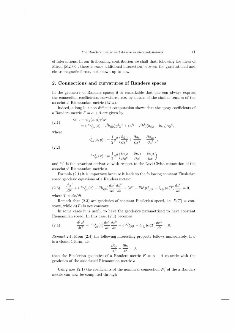
of interactions. In our firthcoming contribution we shall that, following the ideas ofMiron [M2004], there is some additional interaction between the gravitational andelectromagnetic forces, not known up to now.
2. Connections and curvatures of Randers spaces
In the geometry of Randers spaces it is remarkable that one can always expressthe connection coefficients, curvatures, etc. by means of the similar tensors of theassociated Riemannian metric (M,a).
Indeed, a long but non difficult computation shows that the spray coefficients ofa Randers metric F = α+ β are given by
Gi : = γijk(x, y)yiyj
= ( aγijk(x) + libj|k)yjyk + (aij − libj)(bj|k − bk|j)αyk,
(2.1)
where
γijk(x, y) : =
12gil(∂gjl
∂xk+∂gkl
∂xj− ∂gjk
∂xl
),
aγijk(x) : =
12ail(∂ajl
∂xk+∂akl
∂xj− ∂ajk
∂xl
),
(2.2)
and “|” is the covariant derivative with respect to the Levi-Civita connection of theassociated Riemannian metric a.
Formula (2.1) it is important because it leads to the following constant Finslerianspeed geodesic equations of a Randers metric:
d2xi
dt2+ ( aγi
jk(x) + libj|k)dxj
dt
dxk
dt+ (aij − libj)(bj|k − bk|j)α(T )
dxk
dt= 0,(2.3)
where T = dx/dt.Remark that (2.3) are geodesics of constant Finslerian speed, i.e. F (T ) = con-
stant, while α(T ) is not constant.In some cases it is useful to have the geodesics parametrized to have constant
Riemannian speed. In this case, (2.3) becomes
d2xi
dt2+ aγi
jk(x)dxj
dt
dxk
dt+ aij(bj|k − bk|j)α(T )
dxk
dt= 0.(2.4)
Remark 2.1. From (2.4) the following interesting property follows immediately. If βis a closed 1-form, i.e.
∂bjxi
− ∂bixj
= 0,
then the Finslerian geodesics of a Randers metric F = α + β coincide with thegeodesics of the associated Riemannian metric a.
Using now (2.1) the coefficients of the nonlinear connection N ij of the a Randers
metric can now be computed through
42 H. Shimada, S. V. Sabau, and R. S. Ingarden
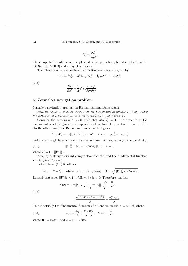
N ij =
∂Gi
∂yj.
The complete formula is too complicated to be given here, but it can be found in[BCS2000], [M2003] and many other places.
The Chern connection coefficients of a Randers space are given by
Γijk = aγi
jk − gil(AljsNsk −AjksN
sl +AklsN
sj )
=∂N i
j
∂yk+
12gitys
∂2Nst
∂yj∂yk.
(2.5)
3. Zermelo’s navigation problem
Zermelo’s navigation problem on Riemannian manifolds reads:Find the paths of shortest travel time on a Riemannian manifold (M,h) under
the influence of a transversal wind represented by a vector field W .Consider the vectors u ∈ TxM such that h(u, u) = 1. The presence of the
transversal wind W gives by composition of vectors the resultant v := u + W .On the other hand, the Riemannian inner product gives
h(v,W ) = ||v||h · ||W ||h · cos θ, where ||y||2h = h(y, y)
and θ is the angle between the directions of v and W , respectively, or, equivalently,
||v||2h − (2||W ||h cos θ)||v||h − λ = 0,(3.1)
where λ := 1 − ||W ||2h.Now, by a straightforward computation one can find the fundamental function
F satisfying F (v) = 1.Indeed, from (3.1) it follows
||v||h = P +Q, where P := ||W ||h cos θ, Q :=√||W ||2h cos2 θ + λ.
Remark that since ||W ||h < 1 it follows ||v||h > 0. Therefore, one has
F (v) = 1 =||v||h 1P +Q
= ||v||h Q− P
Q2 − P 2
=
√[h(W, v)]2 + ||v||2hλ
λ− h(W, v)
λ.
(3.2)
This is actually the fundamental function of a Randers metric F = α+ β, where
aij :=hij
λ+Wi
λ
Wj
λ, bi := −Wi
λ,(3.3)
where Wi = hijWj and λ = 1 −W iWi.
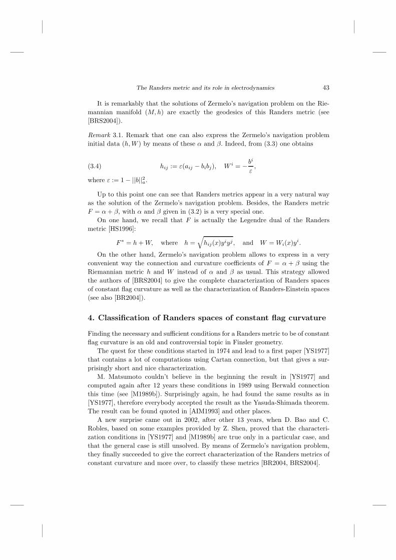
The Randers metric and its role in electrodynamics 43
It is remarkably that the solutions of Zermelo’s navigation problem on the Rie-mannian manifold (M,h) are exactly the geodesics of this Randers metric (see[BRS2004]).
Remark 3.1. Remark that one can also express the Zermelo’s navigation probleminitial data (h,W ) by means of these α and β. Indeed, from (3.3) one obtains
hij := ε(aij − bibj), W i = −bi
ε,(3.4)
where ε := 1 − ||b||2a.
Up to this point one can see that Randers metrics appear in a very natural wayas the solution of the Zermelo’s navigation problem. Besides, the Randers metricF = α+ β, with α and β given in (3.2) is a very special one.
On one hand, we recall that F is actually the Legendre dual of the Randersmetric [HS1996]:
F ∗ = h+W, where h =√hij(x)yiyj , and W = Wi(x)yi.
On the other hand, Zermelo’s navigation problem allows to express in a veryconvenient way the connection and curvature coefficients of F = α + β using theRiemannian metric h and W instead of α and β as usual. This strategy allowedthe authors of [BRS2004] to give the complete characterization of Randers spacesof constant flag curvature as well as the characterization of Randers-Einstein spaces(see also [BR2004]).
4. Classification of Randers spaces of constant flag curvature
Finding the necessary and sufficient conditions for a Randers metric to be of constantflag curvature is an old and controversial topic in Finsler geometry.
The quest for these conditions started in 1974 and lead to a first paper [YS1977]that contains a lot of computations using Cartan connection, but that gives a sur-prisingly short and nice characterization.
M. Matsumoto couldn’t believe in the beginning the result in [YS1977] andcomputed again after 12 years these conditions in 1989 using Berwald connectionthis time (see [M1989b]). Surprisingly again, he had found the same results as in[YS1977], therefore everybody accepted the result as the Yasuda-Shimada theorem.The result can be found quoted in [AIM1993] and other places.
A new surprise came out in 2002, after other 13 years, when D. Bao and C.Robles, based on some examples provided by Z. Shen, proved that the characteri-zation conditions in [YS1977] and [M1989b] are true only in a particular case, andthat the general case is still unsolved. By means of Zermelo’s navigation problem,they finally succeeded to give the correct characterization of the Randers metrics ofconstant curvature and more over, to classify these metrics [BR2004, BRS2004].

44 H. Shimada, S. V. Sabau, and R. S. Ingarden
After some long computations one obtains
Theorem 4.1. ([BR2004]; constant flag curvature characterization). Let F = α+β
be a strongly convex Randers metric. Then (M,F ) is of constant flag curvature Kif and only if there exists a constant σ such that:
• the Basic Equation
lieik + biθk + bkθi = σ(aik − bibk)(4.1)
• the Curvature EquationaRhijk = ξ(aijahk − aikahj)
− 14aijcurl
thcurltk +
14aikcurl
thcurltj
+14ahjcurl
ticurltk − 1
4ahkcurl
ticurltj
− 14curlijcurlhk +
14curlikcurlhj +
12curlhicurljk
(4.2)
hold, where
lieij := bi|j + bj|i, curlij := bi|j − bj|i,
θj := bicurlij , θi := θjaij, curlij := curlkja
ik,
ξ := (K − 316σ2) + (K +
116σ2)||b||a − 1
4θiθi.
(4.3)
We have used here the notations lieij and curlij used in [BR2004]. Remark thatthese are actually the two times of rij and sij used in [BCS2007, M1989b].
In the same way one has
Theorem 4.2. ([BR2004]; characterization of Randers–Einstein metrics). Let F =α + β be a strongly convex Randers metric. Then (M,F ) is an Einstein manifoldwith Ricci scalar Ric(x) if and only if
• the Basic Equation
lieik + biθk + bkθi = σ(aik − bibk)(4.4)
• the Ricci Curvature Equation
aRicik = (aik + bibk)Ric(x) − 14aikcurl
hjcurlhj − 12curlji curljk
− (n− 1){ 116σ2(3aik − bibk) +
14θiθk} +
14
(θi|k + θk|i)(4.5)
are satisfied for some constant σ.
We remark that Theorem 4.1 is the corrected form of the Yasuda-Shimada theo-rem. The original result in [YS1977] coincides with the one in Theorem 1 under thecondition curlij = 0.
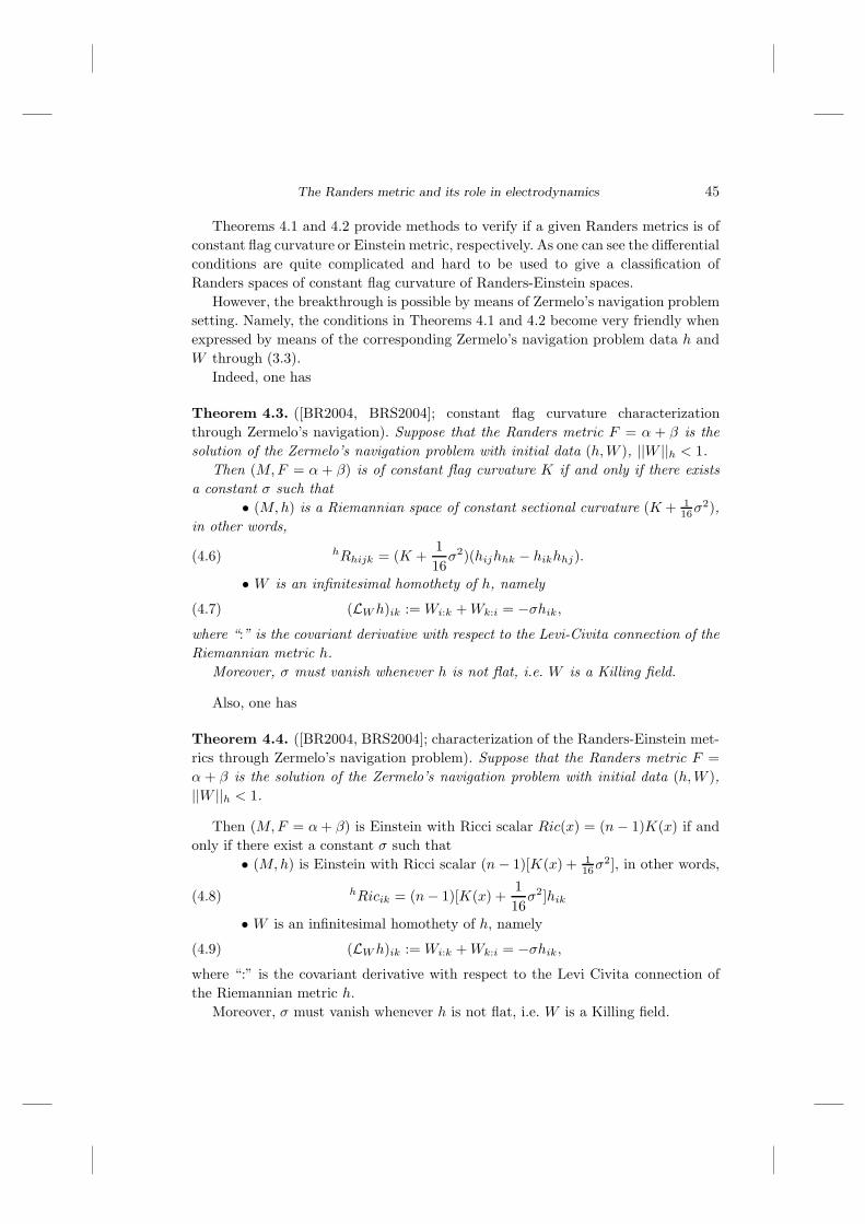
The Randers metric and its role in electrodynamics 45
Theorems 4.1 and 4.2 provide methods to verify if a given Randers metrics is ofconstant flag curvature or Einstein metric, respectively. As one can see the differentialconditions are quite complicated and hard to be used to give a classification ofRanders spaces of constant flag curvature of Randers-Einstein spaces.
However, the breakthrough is possible by means of Zermelo’s navigation problemsetting. Namely, the conditions in Theorems 4.1 and 4.2 become very friendly whenexpressed by means of the corresponding Zermelo’s navigation problem data h andW through (3.3).
Indeed, one has
Theorem 4.3. ([BR2004, BRS2004]; constant flag curvature characterizationthrough Zermelo’s navigation). Suppose that the Randers metric F = α + β is thesolution of the Zermelo’s navigation problem with initial data (h,W ), ||W ||h < 1.
Then (M,F = α + β) is of constant flag curvature K if and only if there existsa constant σ such that
• (M,h) is a Riemannian space of constant sectional curvature (K + 116σ
2),in other words,
hRhijk = (K +116σ2)(hijhhk − hikhhj).(4.6)
• W is an infinitesimal homothety of h, namely
(LW h)ik := Wi:k +Wk:i = −σhik,(4.7)
where “:” is the covariant derivative with respect to the Levi-Civita connection of theRiemannian metric h.
Moreover, σ must vanish whenever h is not flat, i.e. W is a Killing field.
Also, one has
Theorem 4.4. ([BR2004, BRS2004]; characterization of the Randers-Einstein met-rics through Zermelo’s navigation problem). Suppose that the Randers metric F =α + β is the solution of the Zermelo’s navigation problem with initial data (h,W ),||W ||h < 1.
Then (M,F = α+ β) is Einstein with Ricci scalar Ric(x) = (n− 1)K(x) if andonly if there exist a constant σ such that
• (M,h) is Einstein with Ricci scalar (n− 1)[K(x) + 116σ
2], in other words,
hRicik = (n− 1)[K(x) +116σ2]hik(4.8)
• W is an infinitesimal homothety of h, namely
(LW h)ik := Wi:k +Wk:i = −σhik,(4.9)
where “:” is the covariant derivative with respect to the Levi Civita connection ofthe Riemannian metric h.
Moreover, σ must vanish whenever h is not flat, i.e. W is a Killing field.
46 H. Shimada, S. V. Sabau, and R. S. Ingarden
It is remarkable that Theorem 4.3. leads to the complete classification of Randersmetrics of constant flag curvature.
Indeed, for each three standard Riemannian space forms (spherical, Euclideanand hyperbolic) one should find a W that satisfies (4.7). The complete list of allow-able vectors can be found in [BRS2004].
Remark 4.1. Using in the particular case of CP2 one can easily construct a Randers-
Einstein metric of Ricci constant curvature Ricc = 6 (see [Sa2004]).
Remark 4.2. Recall that an odd dimensional manifold M is said to have an almostcontact structure (ϕ, ξ, η) if ϕ, ξ and η are a tensor field of type (1,1), a vectorfield and an 1-form on M , respectively, satisfying
η(ξ) = 1, ϕ2X = −X + η(X)ξ
for any vector field X on M . There exists always a Riemannian metric a on M
compatible with an almost contact structure, i.e.
a(ϕX,ϕY ) = a(X,X) − η(X)η(Y ),
for any vector fields X , Y on M . In this case M is said to have an almost contactmetric structure (ϕ, ξ, η, a).
One can remark that on an odd dimensional manifold M with the almost contactmetric structure (ϕ, ξ, η, a), we can construct an (α, β) metric F = F (α, β) by taking
α =√aij(x)yiyj , β = ηi(x)yi,(4.10)
where ηi(x) are the coefficients of the 1-form η. Remark that in this case ||b||a = 1, sothe metric is not strongly convex anymore. In some cases this problem can be solvedby scaling properly the linear 1-form β, for example one can consider β : εηi(x)yi,0 < ε < 1. But this is not always possible.
In particular, one can consider the Randers metric F = α + β with α and β
given above. This construction and a classification theorem of connected almostcontact Riemannian manifolds whose automorphism group has maximal dimensionleads to a method to construct concrete examples of Randers metrics of constantflag curvature. Remark that many of these metrics are not strongly convex (because||b||a = 1), but only regular. Therefore they are not in the classification given in[BRS2004].
References
[AIM1993] P. L. Antonelli, R. S. Ingarden, and M. Matsumoto, The Theory of Sprays andFinsler spaces with Applications in Physics and Biology, Kluwer Acad. Publ., FTPH58, 1993.
[A2006] G. S. Asanov, Finsler-Finsleroid space with Berwald and Landsberg conditions,Manuscript (2006).
[B2007] D. Bao, On two curvature-driven problems in Riemann-Finsler Geometry, to ap-pear in Advanced Studies in Pure Mathematics, Tokyo, 2007.
The Randers metric and its role in electrodynamics 47
[BR2003] D. Bao and C. Robles, On Randers space of constant flag curvature, Rep. onMath, Phys., 51 (2003), 9–42.
[BR2004] D. Bao and C. Robles, Ricci and flag curvatures in Finsler Geometry, in the vol-ume A Sampler of Riemann-Finsler Geometry, MSRI, vol. 50, Cambridge UniversityPress, 2004, 197–259.
[BCS2000] D. Bao, S. S. Chern, and Z. Shen, An Introduction to Riemann-Finsler Geome-try, Springer, GTM 200, 2000.
[BCS2007] S. Bacso, X. Cheng, and Z. Shen, Curvature Properties of (α, β)-metrics, to ap-pear in Advanced Studies in Pure Mathematics, Tokyo, 2007.
[BBCS2004] D. Bao, R. L. Bryant, S. S. Chern, Z. Shen, A Sampler of Riemann-Finsler Ge-ometry, MSRI Publishers, Vol. 50, 2004.
[BRS2004] D. Bao, C. Robles, and Z. Shen, Zermelo navigation on Riemannian manifolds,J. Diff. Geom., 66 (2004), 377–435.
[Br1997] R. Bryant, Projectively flat Finsler 2-spheres of constant curvature, Selecta Math.,New Series, 3 (1997), 161–204.
[C2] C. Caratheodory, Uber eine spezielle Metrik, die in der Theorie der analytischenFunktionen auftritt, Atti Pontificia Acad. Nuovi Lincei 80 (1927), 135–141.
[F1918] P. Finsler, Uber Kurven uund Fl’achen in allgemeinen Raumen, Dissertation,Gottingen 1918; 2nd. ed. Birkhauser, Basel 1951.
[HSS2004] I. Hasegawa, V. S. Sabau, and H. Shimada, Randers spaces of constant flag cur-vature induced by almost contact metric structures, Hokkaido Math. Jour., Vol. 33(2004), 215–232.
[HS1996] D. Hrimiuc and H. Shimada, On the L-duality between Lagrange and Hamiltonmanifolds, Nonlinear World 3 (1996), 613–641.
[I1957] R. S. Ingarden, On the geometrically absolute optical representation in the electronmicroscope, Trav. Soc. Sci. Lettr. Wroc�law, B 45 (1957), 60 p.
[K2006] L. Kozma, Private communication, 2006.
[L1950] R. K. Luneburg, The metric of binocular visual space, J. Opt. Soc. Am. 40 (1950),624–625.
[L1964] —, Mathematical Theory of Optics, mimeographed notes, Braun University, Prov-idence, RI 1944; Univ. of California Press, Berkeley, CA 1964.
[�L1986] J. �Lawrynowicz, Variationsrechnung und Anwendungen, Springer, Berlin-Heidelberg 1986.
[�L2005] —, Quaternions and fractals vs. Finslerian geometry. I. Quaternion-based modi-fications of the Cayley-Dickson process, Bull. Soc. Sci. Lettres �Lodz 55 Ser. Rech.Deform. 47 (2005), 83–98.
[�LRW2003] —, W. A. Rodrigues, and L. Wojtczak, Stochastical electrodynamics in Clifford-analytical formulation related to entropy-depending structures, ibid. 53 Ser. Rech.Deform. 41 (2003), 69–87.
[M1996] M. Matsumoto, Remarks on Berwald and Landsberg spaces, Contemporary Math-ematics, Vol. 196 (1996), 79–82.
[M1989a] M. Matsumoto, A slope of a mountain is a Finsler surface with respect to a timemeasure, J. Math. Kyoto Univ., 29 (1), (1989), 17–25.
[M1989b] M. Matsumoto, Randers spaces of constant curvature, Rep. on Math, Phys., 28(1989), 249–261.
[M2003] M. Matsumoto, Finsler Geometry in the 20-th Century, Handbook of Finsler Ge-ometry, 1, 2, Ed. P.L. Antonelli, 2003, 557–966.

48 H. Shimada, S. V. Sabau, and R. S. Ingarden
[M2004] R. Miron, The geometry of Ingarden spaces, Rep. Math. Phys. 54 (2004), 131–147.
[MSY2006] X. Mo, Z. Shen, and C. Yang, Some constructions of projectively flat Finslermetrics, Science in China: Series A Math., 49(5), 2006, 703–714.
[vN1927] J. von Neumann, Thermodynamik quantummechanischer Gesamtheit, Gott.Nachr. 1 (1927), 273–291; reprinted in his Collected Works, vol. I, Pergamon Press,Oxford-London-New York-Paris 1961, pp. 236–254.
[vN1955] —, Mathematical Foundations of Quantum Mechanics, Princeton Univ. Press,Priceton, NJ 1955.
[PT2004] J. C. A. Paiva, and A. C. Thompson, Volumes on normed and Finsler spaces, ASampler of Riemann-Finsler Geometry, MSRI Publishers, Vol. 50, 2004, 1–48.
[R1941] G. Randers, On an asymmetric metric in the four-space of general relativity, Phys.Rev. (2)59 (1941), 195–199.
[Sa2004] V. S. Sabau, Randers metrics on CP 2, Periodica Math. Hungarica, 48(1-2)(2004), 25–31.
[SaS2001] V. S. Sabau, and H. Shimada, Classes of Finsler spaces with (α, β)-metrics, Rep.on Math, Phys., 47 (2001), 31–48.
[SaS2003] V.S. Sabau, and H. Shimada, Errata for the paper “Classes of Finsler spaces with(α, β)-metrics”, Rep. on Math, Phys., 47 (2001), 31–48; Rep. on Math, Phys., 51(2003), 149–152.
[S2001] Z. Shen, Lectures in Finsler Geometry, World Scientific, Singapore, 2001.
[Shim2004] H. Shimada, Short review of Yasuda-Shimada theorem and related topics, Peri-odica Math. Hungarica, Vol. 48 (2004), 17–24.
[SSa2005] H. Shimada and V. S. Sabau Introduction to Matsumoto metric, Nonlinear Anal-ysis, 63 (5-7) (2005), e165–e168.
[SSI2008] H. Shimada, V. S. Sabau, and R. S. Ingarden, The (α, β)-metric for Finsler spaceand its role in thermodynamics, Bull. Soc. Sci. Lettres �Lodz 58 Ser. Rech. Deform.57 (2008), 25–38.
[T1977] W. Thirring, Lehrbuch der mathematischen Physik, Band 1. Klassische dynamischeSysteme, Springer, Wien-New York 1977; Polish transl. by P. Kielanowski, PWN,Warszawa 1985.
[YS1977] H. Yasuda and H. Shimada, On Randers spaces of scalar curvature, Rep. on Math.Phys., 11 (1977), 347–360.
Hideo Shimada and Sorin Vasile Sabau Roman Stanis�law Ingarden
Department of Mathematics Institute of Physics
Hokkaido Tokai University Nicolaus Copernicus University
5-1 Minamisawa, Minami-ku Grudziadzka 5, PL-87-100 Torun, Poland
Sapporo, 005-8601, Japan e-mail: [email protected]
e-mails: [email protected]
Presented by W�lodzimierz Waliszewski at the Session of the Mathematical-PhysicalCommission of the �Lodz Society of Sciences and Arts on October 29, 2008

The Randers metric and its role in electrodynamics 49
METRYKA RANDERSA I JEJ ZNACZENIEW ELEKTRODYNAMICE
S t r e s z c z e n i eW pracy zwracamy najpierw uwage na istotna role metryki Randersa przy rozwaaniu la-
granzianu relatywistycznego, co ilustrujemy przez uwzglednienie dodatkowych oddzia�lywanmiedzy si�lami grawitacyjnymi i elektromagnetycznymi. W powiazaniu z koneksjami i krzy-wiznami przestrzeni Randersa rozpatrujemy zagadnienie nawigacji Zermelo, a nastepnieklasyfikacji przestrzeni Randersa o sta�lej krzywiznie flagowej.

PL ISSN 0459-6854
B U L L E T I NDE LA SOCIETE DES SCIENCES ET DES LETTRES DE �LODZ
2008 Vol. LVIII
Recherches sur les deformations Vol. LVII
pp. 51–56
Roman Stanis�law Ingarden and Julian �Lawrynowicz
FINSLER GEOMETRY AND PHYSICS.MATHEMATICAL OVERVIEW
Summary
The mathematical background for studying the influence of the Finsler geometry onphysics has to take into account the modern bundle-theoretic approach which comes back to:– 1. Quaternions, noncommutativity, and C∗-algebras; – 2. Algebraic possibilities (quater-nions, octonions, sedenions); – 3. Quaternion-based modifications of the Cayley-Dicksonprocess; – 4. Noncommutative hypercomplex analysis and C∗-algebras generated by isome-tries; – 5. Graded fractal bundles related to quaternionic structure; – 6. Isospectral defor-mations in complex Finslerian quantum mechanics; – 7. Clifford-analytical description ofquantum-mechanical gauge theories; – 8. Jordan algebras and special Jordan algebras.
With the help of such preparation, the mathematical content of studying the influenceof the Finsler geometry on physics can naturally be divided into three stages: – I. Randersgeometry; – II. Lagrange geometry; – III. Noncommutative associative and commutativenonassociative Finsler geometries.
0. After more than 70 years of relatively slow development Finsler geometry isnow a modern subject with a large body of theorems and techniques, and has math-ematical content comparable to any field of modern differential geometry. We believe“the world is Finslerian” in a true sense and we can show this in our applicationsin thermodynamics, electrodynamics, optics, and classical and quantum mechanics[AIM].
In particular one can define some Finsler spaces, e.g. quantum Randers spacesas being a special case of a noncommutative associative (Gelfald-Connes) geometry,but together with its “strongly dual” or “antidual” real commutative nonassociative(special Jordan) geometry [I].
The Finsler geometrical approach to gauge theories yields the field theory con-taining solitons as solutions of field equations. It is then natural to distinguish static,

52 R. S. Ingarden and J. �Lawrynowicz
dynamic, probabilistic, and quantum Finsler spaces including, because of space-time,complex Finsler structures.
In quantum physics energy, in general, does not commute with time, but thisproblem is difficult because it belongs to the “no-men’s field” between nonrelativisticquantum mechanics and quantum field theory [I�L].
1. Mathematically, as far as the first direction (1.) is concerned, our task causesthe following demands [�L1]:
• Relationship with A. Connes’ vision of noncommutative geometry.
• The role of the Gelfand condition
‖SS∗‖ = ‖S‖2
for Banach algebras equipped with a star operation.
• How to multiply triplets?
• Relationship with the Jordan algebra, especially with a new commutative mul-tiplication
A ◦B =12
(AB +BA).
• The role of the anticommuting generators of H. Grassmann:
ejek + ekej = 0, e2j = 0.
2. In the second direction we have to answer the questions [�L1]:
◦ How to improve nonassociative octonions?
◦ How to reduce the dimension 128 generated by sedenions?
◦ How to make the algebra of sedenions a division algebra?
3. In the third direction we have to look for [�L1]:
• Relationship with the five-dimensional Ka�luza-Klein geometry.
• Analysis of algebraic possibilities round the four- and five-dimensional space-times, and their higher-dimensional analogues.
• “Matrix numbers” proper for quantum physics when quantizing the geometry.
4. In the fourth direction we have to discuss [�L2]:
◦ Consequences of the theorem of Gelfand and Naımark [GN] saying that thecategory of locally compact topological spaces is equivalent to the category ofabelian c∗-algebras.
◦ Quantum mechanics vs. noncommutative geometry.
◦ Interesting examples of noncommutative spaces.

Finsler geometry and physics. Mathematical overview 53
5. In the fifth direction we have to outline [�L2]:
• The role of “commutative”, but highly singular structures, like fractal sets, inthe Randers geometry framework.
• Duality in relation to quaternion-based construction of structure fractals andin relation to the corresponding algebraic (twistor-like) structures with specificharmonic forms and Dolbeault cohomology groups.
• Antiduality of structure fractals and twistor-like structures analogous to thatappearing in the case of a short magnetostatic lens.
6. In the sixth direction we have to describe [�L3]:
◦ Solutions in Finsler quantum mechanics.
◦ Isospectral deformations in quantum mechanics.
◦ Real or complex numbers and real, complex or quaternionic representation ofgeneral quantum mechanics.
7. In the seventh direction we have to study [�L3]:
• Finsler geometry of holomorphic and projectivized bundles.
• Supercomplex structures in complex Finslerian quantum mechanics.
• Hurwitz-pair description of gauge theories.
8. In the eight direction we have to clarify [�L3]:
◦ Von Neumann’s theorem and importance of the quantum-mechanical formal-ism in terms of P. Jordan’s algebras.
◦ Jordan skew lattices vs. Finslerian geometry.
◦ Jordan theory of Cayley quantities vs. Finslerian geometry.
9. With the help of 1. and 2. one is prepared to a deeper understanding of theRanders geometry and Lagrange geometry including Miron’s geometry of Ingardenspaces [M]. The Randers metric is of the form
F (x, y) = α(x, y) + β(x, y),
whereα(x, y) =
√aij(x)yiyj
is a Riemannian metric andβ(x, y) = bi(x)yi
is a linear one-form. A Lagrangian is a smooth real function defined on the entiremanifold TM fibred over a smooth manifold M . The geometrization of Lagrangians

54 R. S. Ingarden and J. �Lawrynowicz
involves in a high degree the geometry of TM and results in the so-called Lagrangegeometry. The idea of R. S. Ingarden developed by R. Miron consists in consideringa general Randers space together with a Lorentz nonlinear connection.
With the help of 3.–8. one gets ready to a deeper understanding of noncommu-tative associative and commutative nonassociative Finsler geometries.
10 (I). When considering the influence of the Randers geometry on physics thefollowing topics are of a particular interest:
◦ Finsler spaces and metrical connections in the tangent manifolds.
◦ The (α, β)-metrics for Finsler spaces.
◦ The Randers metric and its applications.
◦ Metrical quasi-linear connections for Randers spaces.
◦ Randers geometry, solitons, and complex gauge theories.
◦ Randers and Ka�luza-Klein gauge theories, self-duality and homogeneity.
◦ Randers and Ingarden spaces.
11 (II). When considering the influence of the Lagrange geometry on physicsthe following topics are of a particular interest:
• Lagrange geometry, homogeneous Lagrangians and the related Finsler geome-try.
• Semisprays, nonlinear connections and metrical connections in the Lagrangespaces.
• Generalized Laplacians on Lagrange spaces.
• Inverse problems.
• Lagrangians in dynamical systems.
• Elements of variational calculus. Emmy Noether’s theorem.
• Randers “asymmetrical” metric in the space-time.
• Geometry of the point Finsler spaces.
• General Randers spaces; Randers space forms.
• Miron’s geometry of Ingarden spaces.
12 (III). When considering the noncommutative associative and commutativenonassociative Finsler geometries, the following topics are of a particular interest:
◦ Geometical model of magnetic electron microscope.
◦ Geometrical model of the scanning tunnelling microscope.
◦ Geometrical model of quantum electrodynamics.
Finsler geometry and physics. Mathematical overview 55
References
[AIM] P. L. Antonelli, R. S. Ingarden, and M. Matsumoto, The Theory of Sprays and FinslerSpaces with Applications in Physics and Biology, Kluwer Academic, Dordrecht 1993.
[GN] I. M. Gelfand and M. A. Naımark, On the embedding of normed rings into the ring ofoperators in the Hilbert space [in Russian], Mat. Sb. 12 (1943), 197–213.
[I] R. S. Ingarden, Quantum Randers geometry as noncommutative associative and com-mutative nonassociative geometries, Bull. Soc. Sci. Lettres �Lodz 54 Ser. Rech.Deform. 44 (2004), 7–24.
[I�L] — and J. �Lawrynowicz, Physical and biophysical interpretation of a new model ofopen systems with superluminal velocities, Acta Physicae Superficierum 6 (2004),91–106.
[I�LS] —, —, and O. Suzuki, Superluminal signals and Finslerian physics, Bull. Soc. Sci.Lettres �Lodz 53 Ser. Rech. Deform. 39 (2009), 77–105.
[�L1] J. �Lawrynowicz, Quternions and fractals vs. Finslerian geometry. A. Quaternions,noncommutativity, and C∗-algebras; B. Algebraic possibilities (quaternions, octo-nions, sedenions); 1. Quaternion-based modifications of the Cayley-Dickson process,ibid. 55 Ser. Rech. Deform. 47 (2005), 55–66, 67–82, and 83–98.
[�L2] —, Quaternions and fractals vs. Finslerian geometry. 2. Noncommutative hypercom-plex analysis and C∗-algebras generated by isometries; 3. Graded fractal bundles re-lated to quaternionic structure, ibid. 55 Ser. Rech. Deform. 48 (2005), 47–63 and65–82.
[�L3] —, Quaternions and fractals vs. Finslerian geometry. 4. Isospectral deformationsin complex Finslerian quantum mechanics; 5. Clifford-analytical description ofquantum-mechanical gauge theories; 6. Jordan algebras and special Jordan algebras,ibid. 56 Ser. Rech. Deform. 49 (2006). 35–43, 45–60, and 61–77.
[M] R. Miron, The geometry of Ingarden spaces, Rep. Math. Phys. 54 (2004), 131–147.
Institute of Physics Institute of Physics
Nicolaus Copernicus University Univeristy of �Lodz
Grudziadzka 5, PL-87-100 Torun Pomorska 149/153, PL-90-236 �Lodz
Poland Institute of Mathematics
e-mail: [email protected] Polish Academy of Sciences
�Lodz Branch, Banacha 22, PL-90-238 �Lodz
Poland
e-mail: [email protected]
Presented by Julian �Lawrynowicz at the Session of the Mathematical-Physical Com-mission of the �Lodz Society of Sciences and Arts on December 10, 2008
GEOMETRIA FINSLERA A FIZYKA. SPOJRZENIEMATEMATYCZNE
S t r e s z c z e n i eMatematyczna podstawa studiowania znaczenia geometrii Finslera w fizyce powinna
brac pod uwage nowoczesne podejscie teorii wiazek, ktore opiera sie na nastepujacych

56 R. S. Ingarden and J. �Lawrynowicz
zagadnieniach: – 1. Kwaternionowa nieprzemiennosc i algebry C∗; – 2. Mozliwosci alge-braiczne (kwaterniony, oktoniony, sedeniony); – 3. Modyfikacje procesu Cayley’a-Docksonaoparte na kwaternionach; – 4. Nieprzemienna analiza hiperzespolona i algebry C∗ gene-rowane przez izometrie; – 5. Wiazki fraktali z gradacja odniesione do struktury kwater-nionowej; – 6. Zniekszta�lcenia izospektralne w zespolonej finslerowskiej mechanice kwan-towej; – 7. Kliffordowsko-analityczny opis kwantowo-mechanicznych teorii cechowania; –8. Algebry Jordana i specjalne algebry Jordana.
Z pomoca takiego przygotowania matematyczna zawartosc studium znaczenia geometriiFinslera w fizyce moze byc naturalnie podzielona na trzy etapy: – I. Geometria Randersa;– II. Geometria Lagrange’a; – III. Nieprzemienne �laczne i przemienne nie�laczne geometrieFinslera.
PL ISSN 0459-6854
B U L L E T I NDE LA SOCIETE DES SCIENCES ET DES LETTRES DE �LODZ
2008 Vol. LVIII
Recherches sur les deformations Vol. LVII
pp. 57–61
Leszek Wojtczak
SOME REMARKS ON THE GMR
Summary
The background of the discovery of the GMR for which Albert Fert and Peter Grunbergwere awarded the Nobel Price for physics in 2007 is reviewed. The analogy between themultilayer structure and the magnetic stripe domain structure shows two kinds of conditionsin which GMR can be observed.
My contribution to the present seminar in Bedlewo (2008) is of tutorial character,although it contains some original remarks concerning the properties of the giantmagnetoresistance (GMR), in particular, the relation between the GMR and domainstructure.
First of all I would like to notice that the discovery of the GMR in 1988 is asubject of the Nobel Price in 2007. It is awarded to Albert Fert (Paris) and PeterGrunberg (Julich) for their experimental works leading to the discovery of GMR [1].
Applications of this phenomenon have changed the technology for the productionof the hard disks in order to collect the data. The discovery also plays a major rolein various magnetic sensors as well as for the development of new generations ofelectronics. The use of GMR can be regarded as one of the first evident applicationsin the nanotechnology, which is now called spintronics. The date of opening forspintronics is treated the year 1997, when IBM constructed the commercial read-outhead as the pocket-size device.
The original description of the experimental discovery of GMR was presentedduring the International Conference of Magnetism ICM (1988) in Paris and the In-ternational Colloquium on Magnetic Films and Surfaces (ICMFS 1988) in Le Creusotindependently by two experimental teams headed by Fert and Grunberg, who dis-covered the GMR phenomenon in the conditions of different thin film geometry[2, 3]. The leaders of these teams obtained the Nobel Price in 2007, earlier a presti-

58 L. Wojtczak
gious award of the Magnetic Commission of Union Pure and Applied Physics (UPAP)during the ICM 1994 in Warsaw [4].
The discoveries by Fert and Grunberg of GMR were rapidly recognized by thescientific community. Research in magnetism become fashionable with a rich vari-ety of new scientific and technological possibilities. We can see that the award isvery close to the discoveries of physics leading to technical applications like previousNobel prices for the construction od scanning tunnelling microscope (STM) or hightemperature superconductivity (HTS). However, the present topic, GMR, plays alsoan important role for the pure physics. In the recent 20 years it determines thedirection of the development of experimental and theoretical domains of the funda-mental physics taking into account the quantum nature of the phenomenon as wellas the role of geometry connected with the layered system of finite film thickness.The GMR is a good example of how an expected fundamental scientific discoveryof pure quantum character can quickly give rise to new technologies which open thedoor to new fields of science.
The effect of GMR is a quantum-mechanical phenomenon consisting in the ap-pearance of a giant magnetoresistance in thin multilayers by the change of the mag-netic configurations under the influence of an external magnetic field. The simplestgeometry is determined by the sequences of three layers from which the coveringlayers are ferromegnetic while inside them the spacer layer is non-magnetic. Twoconfigurations are determined by the antiferromagnetic order of two covering layersand by the parallel order of two magnetisations inside the covers.
The conditions which are necessary to produce the giant magnetoresistance in thesystem of the threelayered film are: 1) a change of the angle between the directionsof magnetisation in the ferromagnetic sublayers under the influence of an externalmagnetic field, 2) a geometry which assured the film thickness less than the meanpath of free electrons because the effective interactions should place between boththe covers.
The effect of GMR is connected with an effective scattering probabilities depen-dent on the spin orientations of scattered electrons in two channels with spin up (↑)and down (↓). This picture can be determined by the different densities of electronicspins at the Fermi level which leads to the different values of the resistance in twochannels.
In the case of antiferromagnetic order (↑↓) the sum of currents is the same forboth the channels while in the case of the parallel configuration of magnetisation inthe covers (↑↑) the currents are different. Usually, the transition under the influenceof magnetic field runs from the antiparallel ↑↓ to the parallel configuration (↑↑).Stimulating this transition we can observe the effect of the decrease of resistance,i.e., the effect of GMR.
The pioneering works concerned the samples in the form of superlattices (001)Fe/(001)Cr prepared by means of the molecular beam epitaxy method (MBE). The giantmagnetoresitance (GMR) was found then for thin Fe layers separated by the spacer

Some remarks on the GMR 59
layer of Cr. In the case when the layer thickness is 9 A at the temperature 4.2 K theGMR decreased by the factor 2 in the field 2 T.
The electrical resistance of the sample (Fe—Cr—Fe) with the antiferromagnetictype of exchange interaction increases when the layers are magnetized antiferromag-netically. The effect is stronger than the usual anisotropic magnetoresistance. Thephenomenon can be explained in terms of spin fluctuations scattering the conduc-tivity electrons. Thus, the GMR can be described from the physical point of viewby means of the conductivity of electron s in their spin dependent representationthrough the transport from the iron cover, via chromium layer to the next ironcovering layer.
The original discovery of GMR took place when the samples (Fe—Cr—Fe) or themultiplicity of such modulus were used. The Fe films are the ferromagnetic materialwhich is characterized by relatively big cross section for the Hund interaction betweenthe conduction electrons in the band s and the magnetic electrons in the band d
with strong localization. The spacer Cr is an antiferromagnetic layer and its orderingmakes possible a weak magnetization. A similar structure appears in the case of stripemagnetic domains where the domain wall characterized by the angular distributionof magnetisation creates a structure similar to the antifferomagnetic chromium.
We can see that the stripe magnetic domain structure in thin films (e.g. Fe) corre-sponds to the antiferromagnetic configuration multilayers. The electronic resistanceis determined then by the spin-dependent cross section of the scattering process inthe domain sites. The change of the configuration to the ferromagnetic order in thefilm can be performed by the application of the external magnetic field in the direc-tion parallel to the magnetition of one of the domain stripes. The second sequenceof stripes vanishes then. The influence of the external field causes the change of theconfiguration of antiparallelly magnetized stripes to the configuration of parallellymagnetised stripes, it means, the field causes a transition from the domain structureconfiguration to the sample without domains. In this way the field generates theconditions in which the giant magnetoresistance is observed. The basic features ofGMR in domain structure are very similar to those discovered in the multilayered(Fe—Cr—Fe) structure. The difference to a standard GMR system is that the spacerinterlayer consists of the same material as the cover area of collinear magnetic orderbut is characterised by a noncollinear order.
It is worth-while notecing that the considerations of the stripe domain structureeven with the 180◦ domain walls whose thickness is equal to zero are of particularinterest since they reveal GMR. Next, we can see, even in this simple case, that theapplication of an alternative field leads to the oscillations of domain walls which arethen a source of the oscillations of GMR. For the properly chosen characteristicsof eigenfrequencies we can expect a chaotic behaviour of GMR which can be aphenomenon leading to new effects in technological applications [5]. The discovery ofGMR in magnetic multilayers renewed the interest in the magnetoresistive propertiesof domain walls, the domain wall structure influences on the GMR.
60 L. Wojtczak
The dependence of the resistance of iron on the domain structure was measuredexperimentally a long time ago [6]. However, the conditions of these curly experi-ments did not allow a pure contribution due to the domain walls to be distinguishedfrom other phenomena. In this case the theoretical models and their interpretationbring a selection between galvanomagnetic and size effects. The resistivity of domainwall nature can be modelled by spin-dependent tunnelling through the barrier cre-ated by the noncollinear magnetization inside the wall. In this model the influenceof the domain walls on the electronic transport is attributed to the shortening of amean free path due to reflection from the barrier.
The investigations of mutual influence of domain structure on the GMR arerecently developed. In particular, we can see that GMR caused by a Bloch wallin pure Fe samples was considered on the basis of ab initio calculations [6] of theelectronic structure in a superlattice geometry. The restivity of a ferromagnetic wiredepends also on the magnetic domain configuration. The presence of a domain walllowers the resistance in very narrow Ni wires which clearly reveal the effect of adomain wall on the resistance.
The discovery of GMR by Albert Fert and Peter Grunberg and their teams opensthe door to a new field of science. It also contributes to the relations between thedomain wall structure and the GMR. Well controlled domain walls could becomeimportant constituents of future magnetoelectronic devices. The understanding ofdomain walls in confined nanometric geometries is important since those can showa behaviour deviating from their usual bulk properties as, a controlled pinning anda strongly reduced domain wall width. The latter is through to contribute to GMReffect in nanowires [7], nano-constrictions [8] and nano-contacts.
Some remarks concerning the GMR characteristics presented here in their contextto the role of the domain structure show the GMR discovery by Albert Fert and PeterGrunberg in its permanent development.
References
[1] The Discovery of Giant Magnetoresistance Scientific Background on the Nobel Prizein Physics 2007 comiled by the Class for Physics of the Royal Swedish Academy ofSciences, Information Department, Website: www.kva.se
[2] M. N. Baibich, J. M. Broto, A. Fert, F. Nguyen van Dan, F. Petroff, P. Etienne,G. Creuzet, A. Frederich, J. Chazelas, Giant magnetoresistance of (001)Fe/(001)Crmagnetic superlattices, Phys. Rev. Latters 61, 21 (1988), 2472.
[3] G. Binasch, P. Grunberg, F. Saurnbach, W. Zinn, Enhanced magnetoresistance in lay-ered magnetic structures with antiferromagnetic interlayer exchange, Phys. Rev. B,39, 7 (1989), 4828.
[4] A. Fert, P. Grunberg, A. Barthelemy, W. Zinn, Layered magnetic structure interlayerexchange coupling and giant magnetoresistance, J. Mag. Mag. Mater. 140–144(1995), 1.
[5] J. B. A. N. van Hool, K. M. Schep, A. Brataas, G. W. Bauer, P. J. Kelly, Electron trans-port through magnetic domain walls, Phys. Rev. B 39 (1990); E. Rzepecka, The role
Some remarks on the GMR 61
of magnetic domain structure in the case of GMR, (in Polish), Master Thesis, Uni-versity of �Lodz (2008).
[6] B. Yu. Yavorsky, I. Mertig, A. Yu. Perlov, A. N. Yaresko, Giant magnetoresistance dueto a domain wall in Fe: Ab initio study, Phys. Rev. B 66 (2001), 174422.
[7] V. K. Dugaev, J. Barnas, J. Berahdar, V. I. Ivanov, W. Dobrowolski, V. F. Mitin, Mag-netoresistance of a semiconducting magnetic wire with a domain wall, Phys. Rev. B71 (2005), 024430.
[8] N. Kazantseva, R. Wieser, U. Nowak, Transition to linear domain walls in nanostric-tions, Phys. Rev. Lettres 94 (2005), 037206.
Department of Solid State Physics
University of �Lodz
Pomorska 149/153, PL-90-236 �Lodz
Poland
Presented by Leszek Wojtczak at the Session of the Mathematical-Physical Com-mission of the �Lodz Society of Sciences and Arts on October 29, 2008
UWAGI O GIGANTYCZNYM MAGNETOOPORZE
S t r e s z c z e n i eArtyku�l zawiera przeglad niektorych charakterystyk zjawiska magnetooporu giganty-
cznego, ktorego odkrycie w 1988 roku by�lo podstawa przyznania nagrody Nobla z fizykiAlbertowi Fertowi i Peterowi Grunbergowi w 2007 roku.
Zjawisko magnetooporu gigantycznego ma charakter kwantowy i zosta�lo odkryte w cien-kich probkach o geometrii niejednorodnych wielowarstw zelaza i chromu. Analogia strukturynamagnesowania tych warstw do struktury namagnesowania paskowych domen magnety-cznych stwarza niejako dwie kategorie omawianego zjawiska, w ktorym sciany domenoweodgrywaja istotna role w procesie rozpraszania elektronow przewodnictwa przez rozk�ladnamagnesowania w scianach domenowych.


PL ISSN 0459-6854
B U L L E T I NDE LA SOCIETE DES SCIENCES ET DES LETTRES DE �LODZ
2008 Vol. LVIII
Recherches sur les deformations Vol. LVII
pp. 63–67
Leszek Wojtczak and Jerzy Rutkowski
PRESSURE DEPENDENCE OF MELTING TEMPERATURE
Summary
The paper deals with the high pressure dependence of melting temperature in solidswhose effective potential is described by the modified Lennard-Jones potential given interms of the Valenta approach.
The model is based on the Lindemann criterion applied to the mean square displacementof atoms from their equilibrium positions in the case of the effective potential described bythe isothermal compressibility.
The theoretical results are compared with the experimental data for alumminum.
One of the important characteristics of the melting phase transition is the pres-sure influence on the melting temperature.
The survey of this relation is presented in [1] in order to show the role of theanharmonicity contribution and to construct a simple model proposed in terms ofharmonic interactions with effective force constants whose modifications are due tothe method proposed by Valenta [2]. The model originally applied to thin films inits very simple form is based on the harmonic oscillations with the force constantstaken into account as modified by the relation to the elastic constants.
Next, the pressure is assumed in the form of isotropic (hydrostatic) external forceapplied perpendicularly to the whole sample and scaled with respect to the normal(atmospheric) value of pressure: p0 = 1.01325 · 10−4 GPa.
First of all, we take into account the effective potential for solids, e.g. the Lennard-Jones type found in [1] and we modify the mean square displacement of atoms fromtheir equilibrium positions for the rescaled phonon eigenfrequencies in the case of asample under the pressure p. Then the pressure changes the lattice constant R0(p0)of an elementary cell, and a new constantR′
0(p) can be estimated. In those conditionsthe elementary cell volume v0 = R3
0(p0) changes to the volume v′ = R′30(p) leading
to the isothermal compressibility parameter [2]
64 L. Wojtczak and J. Rutkowski
K = − ΔVVΔp
(1)
where
ΔV = R′30(p) −R3
0(p0)(2)
and
Δp = p− p0(3)
hence
R′0 = R0 (1 −KΔp)1/3(4)
describes the deformed lattice constant R′0 which is under the influence of the pres-
sure p while R0 denotes the lattice constant under the normal pressure p0.The potential compressed by the pressure p is then of the form
Φ(R′0) = Φ (R0 + ΔR0)(5)
with
(6a) ΔR0 = R0
[(1 −KΔp)1/3 − 1
]< R0 for p > p0,
and
(6b) ΔR0 > R0 for p < p0.
The relation (5) allows us to consider the renormalized force constants dependent onpressure and to determine the pressure influence on the melting temperature Tm(p).Taking into account the calculations preformed in [1] we can write
Tm(p)Tm(p0)
=Q [x(p)]Q [x(p0)]
(7)
where
x(p) =R′3
0
R30
= [1 −K(p− p0)](8)
and
Q(x) =1
x8/3
[136
1x2
− 76
](9)
found for the Lennard-Jones potential in [1]. Thus
Q [x(p0) = 1] = 1.(10)
Assuming that the compressibility K is originally a constant value K = K0 wecan evaluate it by a comparison the relation (8) with the similar quantity obtainedon the basis of the approach developed by Young Zou and Li-rong Chen [3] inconnection with their calculations of the melting temperature in its dependence onthe pressure close to its normal value.

Pressure dependence of melting temperature 65
Taking into account the formula for the relative volume x(p) in the form [3]
x(p) =V (p)V (p0)
=1 − 1
δ0+1 ln(
1 + δ0+1B0
p)
1 − 1δ0+1 ln
(1 + δ0+1
B0p0
)(11)
we can write it as follows
1 − 1(p− p0)
B0
[1 − 1
δ0+1 ln(
1 + δ0+1B0
p0
)](12)
hence
x(p) = K0 ≈ 1B0
(13)
which allows us to determine the reduced volume (8) and finally to find the melt-ing temperature in its pressure dependence. The parameter δ0 is here Anderson-Gruneisen parameter at the atmospheric pressure and B0 is the isothermal bulkmodulus at the atmospheric pressure and the room temperature.
However, the relation (8) cannot be used for the pressure high enough, wherethe reduced volume is negative which is, of course, in disagreement with the realsituation. In experimental conditions we expect the highest pressure values tendingto infinity for which the reduced volume x(p → p∞) > 0. Thus, the compressibilityK must depend on the pressure. For the purpose of the present paper the simplestform of this dependence gives the relation
K =K0
1 +K1(p− p0)(14)
where K0 denotes now the compressibility K at the normal pressure p = p0 and itis well determined by (13), while K1 is a constant K1 > K0. The compressibility forhigh pressures is then tending to zero, whereas the reduced volume is determined bythe relation
xm =K1 −K0
K1for K1 > K0.(15)
In this way we obtain only one equation for two unknown parameters xm andK1. Thus K1 is a free parameter which allows us to fit the theoretical value of thepressure dependent melting temperature Tm(p) to the experimental data.
We illustrate our procedure by means of the estimation of Tm(p) for the caseof the aluminum sample with Tm(p0) = 933.1 K. A comparison is presented inFig. 1 where the points represent experimental results reported in [4, 5] while thecurves correspond to the theoretical values for K0 = 0.012953 [1/GPa] and K1 =0.053109 [1/GPa], 0.056995 [1/GPa], or 0.060891 [1/GPa]. We can see that thepressure dependent melting temperature calculated theoretically is sensitive to thevalue K1. Taking into account the fitted values of x given by (8) for K describedby (14) we can additionally find the melting temperature due to the Lindemannmelting equation [e.g. 5]:
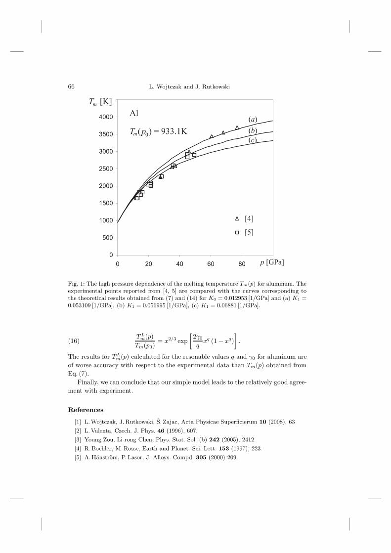
66 L. Wojtczak and J. Rutkowski
Fig. 1: The high pressure dependence of the melting temperature Tm(p) for aluminum. Theexperimental points reported from [4, 5] are compared with the curves corresponding tothe theoretical results obtained from (7) and (14) for K0 = 0.012953 [1/GPa] and (a) K1 =0.053109 [1/GPa], (b) K1 = 0.056995 [1/GPa], (c) K1 = 0.06881 [1/GPa].
TLm(p)Tm(p0)
= x2/3 exp[
2γ0
qxq (1 − xq)
].(16)
The results for TLm(p) calculated for the resonable values q and γ0 for aluminum areof worse accuracy with respect to the experimental data than Tm(p) obtained fromEq. (7).
Finally, we can conclude that our simple model leads to the relatively good agree-ment with experiment.
References
[1] L. Wojtczak, J. Rutkowski, S. Zajac, Acta Physicae Superficierum 10 (2008), 63
[2] L. Valenta, Czech. J. Phys. 46 (1996), 607.
[3] Young Zou, Li-rong Chen, Phys. Stat. Sol. (b) 242 (2005), 2412.
[4] R. Bochler, M. Rosse, Earth and Planet. Sci. Lett. 153 (1997), 223.
[5] A. Hanstrom, P. Lasor, J. Alloys. Compd. 305 (2000) 209.

Pressure dependence of melting temperature 67
Department of Solid State Physics
University of �Lodz
Pomorska 149/153, PL-90-236 �Lodz
Poland
Presented by Leszek Wojtczak at the Session of the Mathematical-Physical Com-mission of the �Lodz Society of Sciences and Arts on December 10, 2008
ZALEZNOSC TEMPERATURY TOPNIENIA OD CISNIENIA
S t r e s z c z e n i ePraca jest poswiecona teoretycznemu opisowi zaleznosci temperatury topnienia od cis-
nienia w modelu Valenty o zmodyfikowanym i izotermicznym wspo�lczynniku scisliwosci.Temperatura topnienia otrzymana w tak okreslonym modelu w zakresie wysokich cis-
nien zosta�la porownana z wynikami doswiadczalnymi dla aluminium. Biorac pod uwageprostote modelu mozemy przyjac, ze dok�ladnosc opisu jest w pe�lni zadowalajaca.

PL ISSN 0459-6854
B U L L E T I NDE LA SOCIETE DES SCIENCES ET DES LETTRES DE �LODZ
2008 Vol. LVIII
Recherches sur les deformations Vol. LVII
pp. 69–78
Hariton M. Polatoglou and Vassiliki Gountsidou
MECHANICAL PROPERTIES OF FUNCTIONALNON-LINEAR MATERIALS WITH NANOSTRUCTURE
Summary
Recently there is a major interest in the discovery of new materials for industrial andcommercial applications and especially for the multifunctional ones. Modeling of the struc-ture of engineering materials, using finite element analysis may reveal specific behavior ofthe component materials and the filling materials, such as mortars, which are the importantboundaries of many engineering materials. It is also possible to include in the study porousmaterials, materials which are not homogenous and have moisture; it is well-known thatcomplicated materials cannot be studied reliably with classical continuum methods. Wemodel the nanoindentation process for fiber-reinforced concrete and study the mechanicalproperties as a function of the distance of a particular fiber.
1. Introduction
The idea of reinforcing soft materials, weak in tension, is simple and well-known fromthe ancient years. Asbestos fibers are known to have been used almost 4,500 years agoto strengthen clay pots [1]. Nowadays the progress in experimental and theoreticalnanomechanics opens new venues in materials science for nanoengineering. Followingthe rapid development of technology in the field of engineering materials there seemsto be a great need to study the structure of thin films in multiple layers, theirmicrohardness and the linear and nonlinear behavior of multifunctional materials[2–4].
Modeling of the mechanical properties using detailed structural representationwith the help of Finite Element Analysis (F.E.A.) may lead to the discovery of specialbehavior not only of the components, but also of the cementitious materials usedfor connecting together the structural materials. [5] Models including random fibers

70 H. M. Polatoglou and V. Gountsidou
with different dimensions and voids can also be constructed. Instruments needed forthe development of complex materials are usually very expensive and only specialistscan make experiments using them.
With the help of computational tools it seems to be relatively easy to performvirtual nanoindentation, a widely known nondestructive method. It is possible tomake models for one or more layers and in any shape or dimension needed. Materialscan be linear or nonlinear. Contour plots of stress or strain, strain-stress curves andeven animation of the indentation can facilitate the study of the properties of thematerials. Recently scientists have started using small distinct reinforcing elementsand try to create and discover proper engineering materials [1]. Nowadays bothmathematical and computational tools and sophisticated experimental techniquesare being used. The complicated cementitious based microstructures are very difficultto be evaluated. Studying the volume and the orientation of the fibres and the volumeand the distribution of the pores or voids, which exist in engineering materials, innano- or micro-scale, very useful conclusions concerning their macroscopic propertiescan be extracted. In recent years multiscale modeling is a promising discipline for thecorrelation of the properties of the nanostructures with those of the bulk crystal [6].
Examining thoroughly the properties of the nanostructures, which are in mostof the cases different from those of the bulk material, the final goal leading to self-repairing structures can be succeeded. The basic material-concrete and the embeddedreinforcing fibers are not homogenous, showing a variety in their mechanical behaviordepending not only from the properties of the component materials but also fromthe percentage and the orientation of the fibers [7]. Specimen of concrete with agiven orientation of fibers, tested under uniaxial tension, confirm the role playedby a locally anisotropic elastic behavior. J. Nemecek et al. [8] targeted a class ofmaterials with the brittle cement-based matrix reinforced by short random fibers,which are called Engineered Cementitious Composites (ECCs). These materials differfrom ordinary cementitious composites by the feature that their microstructure andcomposition are rigorously designed with objective of both acceptable workability inthe fresh state and highly ductile overall behavior under tension in hardened state.
Indentation experiments show the variation of the elastic modulus in relationwith the distance of the fiber from the indentation site. On the other hand compositematerials often contain cavities filled or empty. In particular cementitious materialsalways contain cavities in their structures. Since the size of cavities is similar tothe indenter size it is expected to affect the indentation results. The purpose ofthe present paper is to study the effect of a single fiber on indentation experiment,namely the effect of the distance of the indenter from the fiber on the strain andstress.
2. Method
During the last few years we use indentation based methods in order to find out themechanical properties of materials. Indentation is a rather simple method which can
Mechanical properties of functional non-linear materials with nanostructure 71
be applied on polymeric, ceramic, metallic materials, nanomaterials, bulk metallicmaterials, biomaterials etc and can be applied in multiple length scales. Extractingthe constitutive properties of the materials from the experimental data is not straightforward for multilayered structures or FGMs. On the other hand computational toolslike the Finite Element Analysis (F.E.A.) can greatly facilitate the process [5].
It is worthy to be mentioned that with the help of finite element analysis we canform two kinds of problems: a) the forward problem, when we know the propertiesof the constituent materials and study the indentation process or the mechanicalbehavior of a structure and b) the reverse problem when we study the indentationprocess and find out the behavior and the properties of the material. We can modelthe material whose mechanical properties we are interested in and the indenter inany desired structure. We can apply it on non-homogenous materials, make manyindentation experiments and study them statistically.
In this paper the structure of a material on the top of which there is an embed-ded fiber having the shape of a half cylinder is modeled. Our indenter is a smallorthogonal prism placed in three different positions. We will study the change of theeffective mechanical properties of the material in relation of the distance between theindenter and the fiber. In the present work the simulation took place with the help ofone of the most powerful computational tools of complicated engineering problemsusing finite element analysis named ANSYS. It helps us model complicated struc-tures even with materials with nonlinear behavior and its environment is friendly tothe user. We can model any desired structure in any scale, in three dimensions. Wecan choose automatic three-dimensional meshing as fine as desired, or a manual oneeven finer especially in the surfaces or volumes where a more detailed observationis needed. A variety of contour plots of strain, displacement, stress, etc, graphs ofthe magnitudes studied and animation are some of the benefits of modeling with thehelp of ANSYS.
With ANSYS we created a model of a rectangular material with Young mod-ulus is 750kPa and Poisson ratio is 0.3. We embedded in the middle of the top afiber, harder than the matrix material having the shape of half-cylinder with Youngmodulus is 3.75MPa and Poisson ratio is 0.3. The indenter was assigned a Youngmodulus is 7.5MPa and Poisson ratio is 0.3 too. As shown in the following figures,we immobilized the base of the rectangular material and we selected a proper dis-placement on the top surface of the indenter. In Fig. 1 the model of the material andthe fiber is shown with the indenter far away from the fiber. We constructed modelsfor three different cases according to the position of the indenter in relation with thefiber. In the first place the indenter is on the fiber, in the second one next to thefiber and in the third one away from it. In all studied cases the displacement of thematerial along the perpendicular axis, the stress and the strain are calculated.
In the following plots when the same quantity is depicted, the contour scale isselected to be the same in order to easily compare the figures.
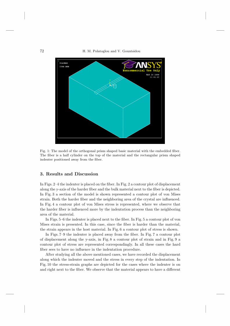
72 H. M. Polatoglou and V. Gountsidou
Fig. 1: The model of the orthogonal prism shaped basic material with the embedded fiber.The fiber is a half cylinder on the top of the material and the rectangular prism shapedindenter positioned away from the fiber.
3. Results and Discussion
In Figs. 2–4 the indenter is placed on the fiber. In Fig. 2 a contour plot of displacementalong the y-axis of the harder fiber and the bulk material next to the fiber is depicted.In Fig. 3 a section of the model is shown represented a contour plot of von Misesstrain. Both the harder fiber and the neighboring area of the crystal are influenced.In Fig. 4 a contour plot of von Mises stress is represented, where we observe thatthe harder fiber is influenced more by the indentation process than the neighboringarea of the material.
In Figs. 5–6 the indenter is placed next to the fiber. In Fig. 5 a contour plot of vonMises strain is presented. In this case, since the fiber is harder than the material,the strain appears in the host material. In Fig. 6 a contour plot of stress is shown.
In Figs. 7–9 the indenter is placed away from the fiber. In Fig. 7 a contour plotof displacement along the y-axis, in Fig. 8 a contour plot of strain and in Fig. 9 acontour plot of stress are represented correspondingly. In all these cases the hardfiber sees to have no influence in the indentation procedure.
After studying all the above mentioned cases, we have recorded the displacementalong which the indenter moved and the stress in every step of the indentation. InFig. 10 the stress-strain graphs are depicted for the cases where the indenter is onand right next to the fiber. We observe that the material appears to have a different
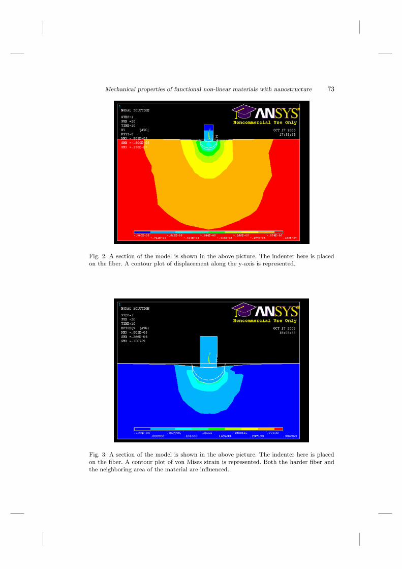
Mechanical properties of functional non-linear materials with nanostructure 73
Fig. 2: A section of the model is shown in the above picture. The indenter here is placedon the fiber. A contour plot of displacement along the y-axis is represented.
Fig. 3: A section of the model is shown in the above picture. The indenter here is placedon the fiber. A contour plot of von Mises strain is represented. Both the harder fiber andthe neighboring area of the material are influenced.
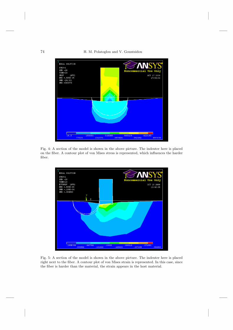
74 H. M. Polatoglou and V. Gountsidou
Fig. 4: A section of the model is shown in the above picture. The indenter here is placedon the fiber. A contour plot of von Mises stress is represented, which influences the harderfiber.
Fig. 5: A section of the model is shown in the above picture. The indenter here is placedright next to the fiber. A contour plot of von Mises strain is represented. In this case, sincethe fiber is harder than the material, the strain appears in the host material.
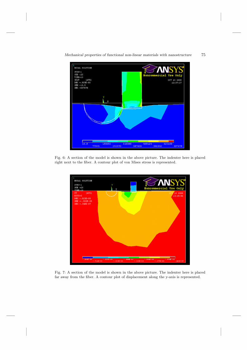
Mechanical properties of functional non-linear materials with nanostructure 75
Fig. 6: A section of the model is shown in the above picture. The indenter here is placedright next to the fiber. A contour plot of von Mises stress is represented.
Fig. 7: A section of the model is shown in the above picture. The indenter here is placedfar away from the fiber. A contour plot of displacement along the y-axis is represented.

76 H. M. Polatoglou and V. Gountsidou
Fig. 8: A section of the model is shown in the above picture. The indenter here is placedfar away from the fiber. A contour plot of von Mises strain is represented. The fiber is farfrom the indentation area and does not have any influence.
Fig. 9: A section of the model is shown in the above picture. The indenter here is placedfar away from the fiber. A contour plot of von Mises stress is represented. The fiber is farfrom the indentation area and does not have any influence.
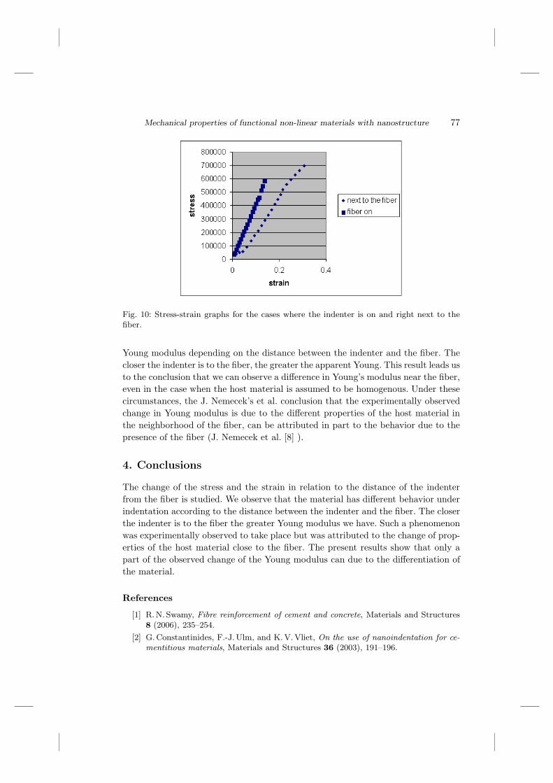
Mechanical properties of functional non-linear materials with nanostructure 77
Fig. 10: Stress-strain graphs for the cases where the indenter is on and right next to thefiber.
Young modulus depending on the distance between the indenter and the fiber. Thecloser the indenter is to the fiber, the greater the apparent Young. This result leads usto the conclusion that we can observe a difference in Young’s modulus near the fiber,even in the case when the host material is assumed to be homogenous. Under thesecircumstances, the J. Nemecek’s et al. conclusion that the experimentally observedchange in Young modulus is due to the different properties of the host material inthe neighborhood of the fiber, can be attributed in part to the behavior due to thepresence of the fiber (J. Nemecek et al. [8] ).
4. Conclusions
The change of the stress and the strain in relation to the distance of the indenterfrom the fiber is studied. We observe that the material has different behavior underindentation according to the distance between the indenter and the fiber. The closerthe indenter is to the fiber the greater Young modulus we have. Such a phenomenonwas experimentally observed to take place but was attributed to the change of prop-erties of the host material close to the fiber. The present results show that only apart of the observed change of the Young modulus can due to the differentiation ofthe material.
References
[1] R. N. Swamy, Fibre reinforcement of cement and concrete, Materials and Structures8 (2006), 235–254.
[2] G. Constantinides, F.-J. Ulm, and K. V. Vliet, On the use of nanoindentation for ce-mentitious materials, Materials and Structures 36 (2003), 191–196.
78 H. M. Polatoglou and V. Gountsidou
[3] E. K. K. Nambiar and K. Ramamurthy, Models for strength prediction of foam con-crete, Materials and Structures 41 (2008), 247–254.
[4] I. Papayianni and M. Stefanidou, Strength-porosity relationships in lime-pozzolanmortars, Construction and Building Materials 20 (2006), 700–705.
[5] Chen. Zhangxin, Finite Element Methods and Their Applications, Springer Verlag,Berlin, Heidelberg 2005.
[6] H. M. Jennings, J. J. Thomas, J. S. Gevrenof, G. Constantinidis, and F.-J. Ulm, Amulti-technique investigation of the nanoporosity cement paste, Cement and ConcreteResearch 37 (2007), 329–336.
[7] O. Bayard and O. Ple, Fracture mechanics of reactive powder concrete:material mod-eling and experimental investigations Engineering, Fracture Mechanics 70 (2003),839–851.
[8] J. Nemecek, P. Kabele, B. Zdenek, Nanoindentation based assessment of microme-chanical properties of fiber reinforced cementitious composite, 6th RILEM Symposiumon Fiber-Reinforced Concretes (FRC)-BEFIB 2004, 20–22 September 2004, Varenna,Italy, 401–410.
Department of Physics
Aristotle University of Thessaloniki
GR-54124 Thessaloniki, Greece
e-mail: [email protected]
Presented by Anna Urbaniak-Kucharczyk at the Session of the Mathematical-Phys-ical Commission of the �Lodz Society of Sciences and Arts on September 23, 2008
W�LASNOSCI MECHANICZNE (WIELO)FUNKCYJNYCHSUROWCOW NIELINIOWYCH Z NANOSTRUKTURA
S t r e s z c z e n i eOstatnio wystepuje zwiekszone zainteresowanie odkryciem nowych surowcow o zasto-
sowaniu przemys�lowym i komercyjnym, a szczegolnie surowcow wielofunkcyjnych. Mode-lujac strukture surowcow technicznych przy uzyciu analizy elementu skonczonego moznaods�lonic specyficzne zachowanie sie sk�ladnikow i elementow uszczelniajacych typu zapraw,ktore sa istotne na brzegach licznych surowcow technicznych. Do przedmiotu badan moznatez w�laczyc surowce porowate, osrodki niejednorodne i nawilzone; jest jednak wiadome,ze skomplikowane materia�ly nie dadza sie rzetelnie zbadac w oparciu o klasyczne metodyciag�le. Autorzy modeluja proces nanoidentacji dla betonu wzmocnionego w�loknami i badajaw�lasnosci mechaniczne w funkcji odleg�losci poszczegolnego w�lokna.

PL ISSN 0459-6854
B U L L E T I NDE LA SOCIETE DES SCIENCES ET DES LETTRES DE �LODZ
2008 Vol. LVIII
Recherches sur les deformations Vol. LVII
pp. 79–87
Giannis Moutsinas and Hariton M. Polatoglou
A DYNAMICAL APPROACH TO POPULATIONSWITH INHERITABLE CHARACTERISTICS
Summary
The process of reproduction in nature is approached by the means of an abstract popu-lation and a simple stochastic algorithm. The algorithm’s results appear to be predictable.When the Mendelian rules of inheritance are being used, natural selection has no effecton the population, all its members are equally qualified for reproduction, and the Hardy-Weinberg principle is found.
1. Introduction
The process of gene inheritance in a population is very complex since a wide listof interactions has to be taken into account, which includes the process of mating,interactions with other species, differences between genders, environmental changesand so forth. A complete analysis of all these seems, if not is, impossible. Howeverit is possible to decompose this process into its parts and try to analyze simplercases [1].
Initially the analysis targeted populations with non-overlapping generations,which required discrete equations [2]. Populations with overlapping generations re-quire continuous equations, which show the time evolution of distribution functions,however this can be avoided by separating the population in age classes [3]. In thesemethods natural selection usually appears only as a mortality or fertility rates. Amechanism to delve deeper natural selection requires the use of game theory. Gametheory allows us to recognize effective intra and inter species strategies, thus under-standing better the forces acting on evolution [4, 5].
In the present work the only mechanism that will be taken into account is themechanism of inheritance. Furthermore the rules of inheritance are generalized and

80 G. Moutsinas and H. M. Polatoglou
they do not need to be those of genetic inheritance. This dictates the use of ageneralized population which is nothing more than a discrete set and does not needto be considered as a biological one.
2. The population
The population is a discrete set of individuals with a set of exclusive characteristics.We assume that each θ has one and only one characteristic. A, with A = {Ai : i ∈{1, 2, . . . , ν}}. Each individual carries a characteristic, which is used to categorizeindividuals into subsets. This population does not interacts with its environment, infact the consept of environment is deprived of meaning. The only thing that changesthe population is the addition of new individuals, which will be called offspringhereon. Offspring carry also a characteristic, which is determined by the characteris-tics of two other individuals, which will be called parents, chosen randomly from thepopulation. Each parent is put back into the population after it has been chosen, sohe may be chosen twice.
Let Θ be the population and θ the individuals that are its members. We defineΘi as subset of Θ containing only individuals with the characteristic Ai, namely θi.We denote by αi their frequencies in Θ, namely the fraction with numerator thecardinality of Θi and denominator the cardinality of Θ, that is
αi =|Θi||Θ| .(1)
Due to the exclusive nature of characteristics we have
Θi
⋂Θj = ∅ when i �= j.
Furthermore all individuals have a characteristic from the set A, so we have
Θ1
⋃Θ2
⋃. . .⋃
Θν = Θ.
This gives us|Θ1| + |Θ2| + . . .+ |Θν | = |Θ|,
thusn∑i=1
αi = 1 .(2)
We now assume that the characteristics are inheritable. This means that we takesteps and add individuals to Θ. These individuals have a characteristic of the set Aaccording to rules we have decided beforehand. These rules will be named rule setof inheritance.
We make the assumption that the fraction of the number of individuals addedto Θ in every step to the cardinality of Θ is a constant and much smaller than 1. Ifwe name N the cardinality of Θ and n the number of individuals added in any step,then ε = n/N is a constant and ε� 1.

A dynamical approach to populations with inheritable characteristics 81
3. The process of change
The fundamental element in this model is inheritance. Inheritance creates the needto choose random individuals from Θ, the parents, and check against the rule set ofinheritance in order to decide the characteristic that the offspring will carry. We willarbitrarily limit the rules by saying that we need only a random pair of individualsand not more. We also assume that we choose θi with probability αi.
An example of rules of inheritance can be the one that states when the firstparent is θ1 and the second θ2, add n/2 θ3 and n/2 θ4. In order to represent ruleslike this, we will use a three dimensional matrix, Λ. It’s elements are symbolized asλijk . This represents the portion of the n individuals added in a step that are θk whenthe first parent is θi and the second θj . It seems natural to assume that λijk = λjik ,however there is no current need for this assumption. By definition we ensure that
λijk ∈ [0, 1].
The previous rule is written as
λ123 = λ12
4 =12.
The assumption that ε is constant dictates thatν∑k=1
λijk = 1 .
We also define pk as the fraction with numerator the mean number of the n
members added that are θk and denominator these n members added. Equivalentlyin equation form
pk =ν∑i=1
ν∑j=1
λijk αiαj .(3)
A useful attribute of pk is∑pk = 1. This can be shown easily
ν∑k=1
pk =ν∑k=1
ν∑i=1
ν∑j=1
λijk αiαj =ν∑i=1
ν∑j=1
(ν∑k=1
λijk αiαj
)
=ν∑i=1
ν∑j=1
(αiαj
(ν∑k=1
λijk
))=
ν∑i=1
ν∑j=1
αiαj
=
(ν∑i=1
αi
)2
= 1 .
We denote the change of a frequency αi, due to the addition of offspring whenthe first parent is θj and the second θk, δαjki , which is δαjki = α′
i − αi, where αi isthe frequency before the addition and α′
i the frequency after. The cardinality of Θi
is denoted by ni. In any given step, in Θi are added λjki n individuals. This gives us
82 G. Moutsinas and H. M. Polatoglou
δαjki = α′i − αi =
ni + λjki n
N + n− niN
=(ni + λjki n)N − ni(N + n)
N(N + n)
=niN + λjki nN − niN − nni
N(N + n)
=λjki nN − nniN(N + n)
=n
N + n
λjki N − niN
.
We define
κ =ε
1 + ε(4)
and with Eq. (1) we have
δαijk = κ(λijk − αk) .(5)
The above equations preserve Eq. (2), hence the normalization of the systemν∑k=1
δαijk =ν∑k=1
κ(λijk − αk
)= κ
(ν∑k=1
λijk −ν∑k=1
αk
)= κ(1 − 1) = 0.
4. Application to biology
Naturally, once the model is set up, one has to investigate whether it gives any usefullresults. Obviously the population that should be used is a biological one. In thesepopulations genes are being inherited, however the genotype is the characteristiceach individual carries. In order to stay in line with the initial assumptions, ourpopulation should have the following attributes.
• There should be no natural selection acting on the population.
• There are no mutations happening that can introduce new genes or alteringone gene to an other existing one.
• There is no migration.
• The individual’s genotype does not change its ability to reproduce.
• The population is sufficiently large.
The first three attributes imply that the frequencies do not change by any othermeans than the addition of offspring. The last two make sure that the assumptionof Paragraph 3, that we choose θi with probability αi, holds.

A dynamical approach to populations with inheritable characteristics 83
4.1. A simple population
The simplest biological population is one with two alleles of one gene, G and g re-spectively. The possible genotypes are three, GG, Gg and gg. We need to constructthe rule set of inheritance, in other words the matrix Λ, and we do so with an ex-tended Punnett square. The extended Punnett square is one with genotypes insteadof genes. One such square is Table 1. The fractions carry the meaning of probability.For example when one parent is Gg and the other GG, then most probably half oftheir offsprings will be GG and the other half will be Gg.
Tab. 1: The extended Punnett square
GG Gg gg
GG GG 12GG+ 1
2Gg Gg
Gg 12GG+ 1
2Gg14GG+ 1
2Gg + 14gg
12Gg + 1
2gg
gg Gg 12Gg + 1
2gg gg
We can now represent genotype GG with A1, Gg with A2 and gg with A3 and Table 1becomes
Tab. 2: System’s rule set of inheritance
A1 A2 A3
A1 A112A1 + 1
2A2 A2
A212A1 + 1
2A214A1 + 1
2A2 + 14A3
12A2 + 1
2A3
A3 A212A2 + 1
2A3 A3
The Λ matrix becomesλ11
1 = λ333 = λ13
2 = λ312 = 1,
λ121 = λ12
2 = λ211 = λ21
2 = λ222 = λ23
2 = λ233 = λ32
2 = λ323 = 1
2 ,
λ221 = λ22
3 = 14 ,
λi31 = λ3i1 = λi13 = λ1i
3 = λ112 = λ33
2 = 0 .
4.2. Prediction
With Λ known, by the definition of pi, Eq. (3), we have
p1 = α21 + α1α2 + 1
4α22,
p2 = 2α1α3 + α1α2 + α2α3 + 12α
22,
p3 = α23 + α2α3 + 1
4α22 .
The above equations can be written as
p1 =(α1 + 1
2α2
)2,
p2 = 2(α1 + 1
2α2
) (α3 + 1
2α2
),
p3 =(α3 + 1
2α2
)2.
(6)
84 G. Moutsinas and H. M. Polatoglou
We define two new quantities. The new quantities, and q, are respectively thefrequencies of genes G and g in the population.
= α1 + 12α2,
q = α3 + 12α2.
(7)
with + q = α1 + α2 + α3 = 1. Eqs. (7) can be written as
dα1
dt= 2 − α1
dα2
dt= 2q − α2(8)
dα3
dt= q2 − α3 .
The quantities and q are constants.d
dt=dα1
dt+
12dα2
dt
= 2 − α1 +12
(2q − α2)
= 2 − α1 + q − 12α2
= (+ q) − (α1 +12α2)
= − = 0 .
The same can be shown for q. This means that the differential Eqs. (8) are in factlinear and their equilibrium point is
α1 = 2,
α2 = 2q,α3 = q2,
(9)
which actually is a family of equilibrium points that form a curve as we shall see.
4.3. Graphical representation
The existence of Eq. (2) reduces by one the number of the differential equations. Inthis specific case the system (8) becomes 2-dimensional. We can visualize this factif we consider that in the 3-dimensional space (α1, α2, α3), the system remains onthe level α1 + α2 + α3 = 1. And since αi have to remain in the interval (0, 1) thesystem lays on the equilateral triangle with vertices the points (1, 0, 0), (0, 1, 0) and(0, 0, 1). We choose a transformation that does not distorts this equilateral triangle.One such transformation is M which transforms (α1, α2, α3) to (v, w) and is definedby
(v
w
)=
( 1√2
0 − 1√2
− 1√6
√23 − 1√
6
)⎛⎝ α1
α2
α3
⎞⎠ .
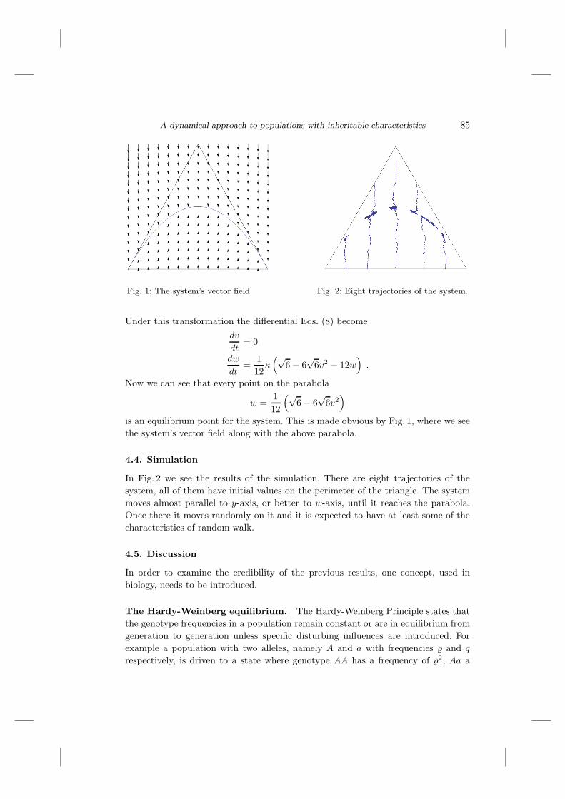
A dynamical approach to populations with inheritable characteristics 85
Fig. 1: The system’s vector field. Fig. 2: Eight trajectories of the system.
Under this transformation the differential Eqs. (8) becomedv
dt= 0
dw
dt=
112κ(√
6 − 6√
6v2 − 12w).
Now we can see that every point on the parabola
w =112
(√6 − 6
√6v2)
is an equilibrium point for the system. This is made obvious by Fig. 1, where we seethe system’s vector field along with the above parabola.
4.4. Simulation
In Fig. 2 we see the results of the simulation. There are eight trajectories of thesystem, all of them have initial values on the perimeter of the triangle. The systemmoves almost parallel to y-axis, or better to w-axis, until it reaches the parabola.Once there it moves randomly on it and it is expected to have at least some of thecharacteristics of random walk.
4.5. Discussion
In order to examine the credibility of the previous results, one concept, used inbiology, needs to be introduced.
The Hardy-Weinberg equilibrium. The Hardy-Weinberg Principle states thatthe genotype frequencies in a population remain constant or are in equilibrium fromgeneration to generation unless specific disturbing influences are introduced. Forexample a population with two alleles, namely A and a with frequencies and q
respectively, is driven to a state where genotype AA has a frequency of 2, Aa a
86 G. Moutsinas and H. M. Polatoglou
frequency of 2q and aa a frequency of q2. Moreover the frequencies, and q, remainconstant [1, 6].
This principle fails to apply in several occasions.
• When mating is non random, for example when one genotype is favored inbreeding or when parts of the population become isolated.
• When there is natural selection in the population, meaning that one genotypeis fitter for survival.
• When a mutation occurs in the population, that changes the one allele to theother.
Comparison. The Hardy-Weinberg Principle’s requirements stay in line with theassumptions made in the beginning of Paragraph 4 and the equilibrium points thatwere found (Eqs. (9)) are those of the Principle. Forthermore we have seen that thefrequencies and q remain constant, exactly as the principal states.
5. Conclusions
The above data show that a population with inheritable characteristics can be sim-ulated by a simple stochastic algorithm, as long as natural selection does not acton it and the members of the population are indifferent to the characteristics theycarry. Furthermore the assumption that the results can be predicted by the use ofthe mean change seems valid, since not only the prediction stays in line with thealgorithm’s results, but it also agrees with what is known from biology.
References
[1] S. Wright, Evolution in Mendelian Populations, University of Chicago, 1930http://www.esp.org/foundations/genetics/classical/holdings/w/sw-31.pdf.
[2] A. W. F. Edwards, Foundations of Mathematical Genetics, Cambridge UniversityPress, Second Edition, 2000.
[3] B. Charlesworth, Evolution in Age-Structured Populations, Cambridge UniversityPress, Second Edition, 1994.
[4] J. M. Smith, Evolution and the Theory of Games, Cambridge University Press, 1982.
[5] J. Hofbauer and K. Sigmund, Evolutionary Games and Population Dynamics, Cam-bridge University Press, 1998.
[6] G. H. Hardy, Mendelian proportions in a mixed population, Science 28 (1908), 49–50,http://www.esp.org/foundations/genetics/classical/hardy.pdf.
[7] R. Grimshaw, Nonlinear Ordinary Differential Equations, CRC Press, 1991.
[8] J. Hale and H. Kocak, Dynamics and Bifurcations, Springer-Verlag, 1991.
[9] G. Iooss and D. D. Joseph, Elementary Stability and Bifurcation Theory, Springer-Verlag, 1997.
[10] M. R. Spiegel, J. J. Schiller and R. A. Srinivasan, Schaum’s Outline of Probability andStatistics, McGraw-Hill, Second Edition, 2000.

A dynamical approach to populations with inheritable characteristics 87
Physics Department
Aristotle University of Thessaloniki
GR-54124 Greece
Presented by Leszek Wojtczak at the Session of the Mathematical-Physical Com-mission of the �Lodz Society of Sciences and Arts on September 23, 2008
PODEJSCIE DYNAMICZNE DO POPULACJIZ DZIEDZICZNYMI CHARAKTERYSTYKAMI
S t r e s z c z e n i eProces reprodukcji w przyrodzie jest przyblizony poprzez abstrakcyjna populacje i pro-
sty algorytm stochastyczny. Okazuje sie, ze jego rezultaty sa przewidywalne. Gdy stosowanesa regu�ly dziedziczenia Mendla, dobor naturalny nie ma wp�lywu na populacje, wszyscyjej cz�lonkowie w rownej mierze kwalifikuja sie do reprodukcji i dochodzimy do zasadyHardy’ego-Weiberga.

PL ISSN 0459-6854
B U L L E T I NDE LA SOCIETE DES SCIENCES ET DES LETTRES DE �LODZ
2008 Vol. LVIII
Recherches sur les deformations Vol. LVII
pp. 89–96
Grzegorz Karwasz
EXPERIMENTAL MODERN PHYSICS:WHY DO WE NEED NEW MATHEMATICS?
Summary
One hundred years or so, it was believed that the knowledge on Physics was completeand only tiny improvements are needed. Soon, Quantum Physics was discovered and theXIX century mathematical apparatus turned out useful in calculations of hydrogen-atomemission spectra and in designing pharmaceutical products, now.
It seems that we may face a similar revolution in the near future. A lot of experimentalevidence in Physics does not find clear theoretical explanations; numerous come to a totalsurprise. We mention here: in Solid State Physics high-T superconductors, in ElementaryParticle Theory – the wide (and apparently) disordered range of quark masses and theCP broken symmetry; in Cosmology – uknown solution of the General Relativity and theproblem of dark mass and energy. With a high probability new ideas from Mathematicsare needed for Physics.
1. Historical outline
The starting point of Quantum Physics is usually identified with the lecture of Planckat Berlin meeting of the Deutschen Physikalischen Gesellschaft on Dec. 14th, 1900,where he put the hypothesis of quanta as the portion of the radiative energy. Incommon understanding it appears to be a kind of ad hoc hypothesis invented byPlanck to avoid the problem with the black-body radiation density spectra in thehigh-frequency range (so called the UV catastrophy). However, a precise inspectionof Planck’s papers proves different.
Planck, searching for the unification between Maxwell-Boltzmann thermodynam-ics and Maxwell electrodynamics, produced several formulae which had predictedpretty well the experimentally measured intensity of radiation. However, at aboutmid October 1900 new measurements differed from Planck’s formulae, even if withthe difference almost impossible to notice. Planck, in several weeks of hard work
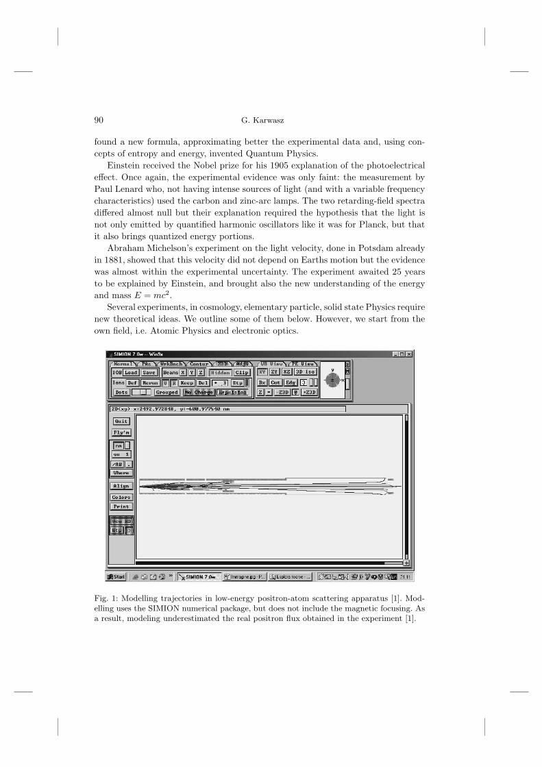
90 G. Karwasz
found a new formula, approximating better the experimental data and, using con-cepts of entropy and energy, invented Quantum Physics.
Einstein received the Nobel prize for his 1905 explanation of the photoelectricaleffect. Once again, the experimental evidence was only faint: the measurement byPaul Lenard who, not having intense sources of light (and with a variable frequencycharacteristics) used the carbon and zinc-arc lamps. The two retarding-field spectradiffered almost null but their explanation required the hypothesis that the light isnot only emitted by quantified harmonic oscillators like it was for Planck, but thatit also brings quantized energy portions.
Abraham Michelson’s experiment on the light velocity, done in Potsdam alreadyin 1881, showed that this velocity did not depend on Earths motion but the evidencewas almost within the experimental uncertainty. The experiment awaited 25 yearsto be explained by Einstein, and brought also the new understanding of the energyand mass E = mc2.
Several experiments, in cosmology, elementary particle, solid state Physics requirenew theoretical ideas. We outline some of them below. However, we start from theown field, i.e. Atomic Physics and electronic optics.
Fig. 1: Modelling trajectories in low-energy positron-atom scattering apparatus [1]. Mod-elling uses the SIMION numerical package, but does not include the magnetic focusing. Asa result, modeling underestimated the real positron flux obtained in the experiment [1].
Experimental Modern Physics: why do we need New Mathematics? 91
2. Electron (and positron) optics
Roman Ingarden in his PhD thesis in 1957 considered the use of new geometry, nowcalled Randers-Ingarden geometry, for modeling motion of electrons in an electronmicroscope. Nowadays, numerical packets allow to model even complex electronoptics, but these programs are not perfect and experimental setting of apparates needsome laboratory skills. We give an example of the recent apparatus for positron-atomscattering from Trento University, in which the setting used [1] differed significantlyfrom those projected: we have “inverted” the optics operation from an accelerating(200 → 2000 eV) to the decelerating (200 → 20 eV) mode.
This in principle is possible, but as the initial energy of positron is 2 eV withthe energy spread of about 1 eV, the numerical modeling, see Fig. 1, gave the verylow beam intensity, say of positrons per second. In spite of this, the convoluted useof the low-intensity, longitudinal guiding magnetic field allowed us to work with ashigh as 10-100 positrons per second counting rate and obtain some intriguing, newphysical results [1].
The numerical packets used, like SIMION, based on Poisson equation (in “nor-mal” 3D space), hardly allow to include effects of the magnetic field, which performsadditional focusing, but with a-quasi resonant conditions (an integer number ofpositron spiraling inside the scattering cell). We question, if the use of more sophis-ticated approach, say Randers-Ingarden geometries would facilitate modelling of thepositron optics in this practical case.
3. Solid State Physics
The quantum Hall effects was discovered in 1980 by Klaus von Klitzing. Work-ing with high magnetic fields he found that at low temperatures the Hall volt-age (perpendicular to the direction of the conduction current and arising fromcurving electron paths in the magnetic field) changes in a step-like manner. Thesuccessive values of the Hall conductance are integer multiples of the constante2/h = 1/(25812.807572 Ω). On this way, the quantum Hall effect allows to measurewith a high precision fundamental constants of nature irrespective of the sampleimperfections. It was shown only recently that quantization of the Hall conductanceresults from topological considerations on the Hamiltonian: under great deformationsof Hamiltonian the curvature of the Hall conductance passes from one topologicalChern number to another [2].
Also recently, new phenomena have been discovered for a class of materials witha high spin-orbit coupling, in which the internal magnetic field substitutes effectsof the external magnetic field. In HgTe-CdTe quantum wells changing the thicknessof the well induces the transition from an insulating state to a phase exhibitingquantum spin Hall effect. It has been recently shown that this change results froma topological quantum phase transition [3].
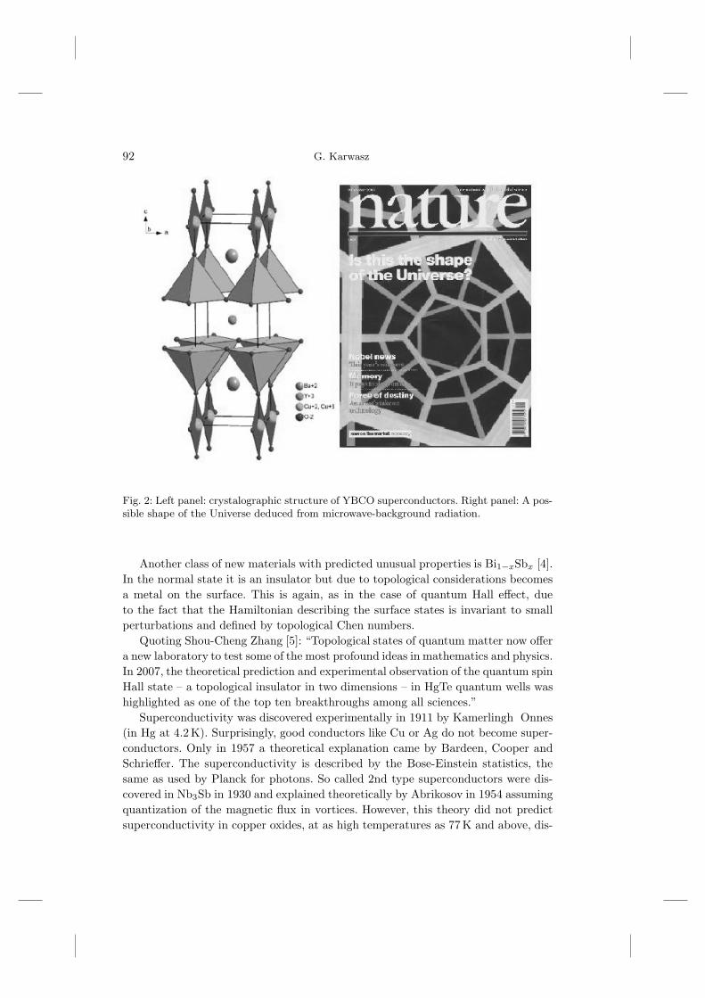
92 G. Karwasz
Fig. 2: Left panel: crystalographic structure of YBCO superconductors. Right panel: A pos-sible shape of the Universe deduced from microwave-background radiation.
Another class of new materials with predicted unusual properties is Bi1−xSbx [4].In the normal state it is an insulator but due to topological considerations becomesa metal on the surface. This is again, as in the case of quantum Hall effect, dueto the fact that the Hamiltonian describing the surface states is invariant to smallperturbations and defined by topological Chen numbers.
Quoting Shou-Cheng Zhang [5]: “Topological states of quantum matter now offera new laboratory to test some of the most profound ideas in mathematics and physics.In 2007, the theoretical prediction and experimental observation of the quantum spinHall state – a topological insulator in two dimensions – in HgTe quantum wells washighlighted as one of the top ten breakthroughs among all sciences.”
Superconductivity was discovered experimentally in 1911 by Kamerlingh Onnes(in Hg at 4.2 K). Surprisingly, good conductors like Cu or Ag do not become super-conductors. Only in 1957 a theoretical explanation came by Bardeen, Cooper andSchrieffer. The superconductivity is described by the Bose-Einstein statistics, thesame as used by Planck for photons. So called 2nd type superconductors were dis-covered in Nb3Sb in 1930 and explained theoretically by Abrikosov in 1954 assumingquantization of the magnetic flux in vortices. However, this theory did not predictsuperconductivity in copper oxides, at as high temperatures as 77 K and above, dis-
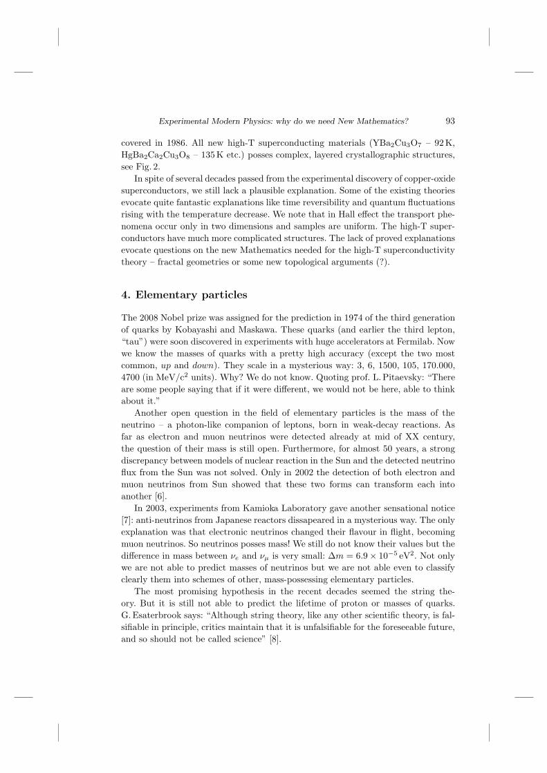
Experimental Modern Physics: why do we need New Mathematics? 93
covered in 1986. All new high-T superconducting materials (YBa2Cu3O7 – 92 K,HgBa2Ca2Cu3O8 – 135 K etc.) posses complex, layered crystallographic structures,see Fig. 2.
In spite of several decades passed from the experimental discovery of copper-oxidesuperconductors, we still lack a plausible explanation. Some of the existing theoriesevocate quite fantastic explanations like time reversibility and quantum fluctuationsrising with the temperature decrease. We note that in Hall effect the transport phe-nomena occur only in two dimensions and samples are uniform. The high-T super-conductors have much more complicated structures. The lack of proved explanationsevocate questions on the new Mathematics needed for the high-T superconductivitytheory – fractal geometries or some new topological arguments (?).
4. Elementary particles
The 2008 Nobel prize was assigned for the prediction in 1974 of the third generationof quarks by Kobayashi and Maskawa. These quarks (and earlier the third lepton,“tau”) were soon discovered in experiments with huge accelerators at Fermilab. Nowwe know the masses of quarks with a pretty high accuracy (except the two mostcommon, up and down). They scale in a mysterious way: 3, 6, 1500, 105, 170.000,4700 (in MeV/c2 units). Why? We do not know. Quoting prof. L. Pitaevsky: “Thereare some people saying that if it were different, we would not be here, able to thinkabout it.”
Another open question in the field of elementary particles is the mass of theneutrino – a photon-like companion of leptons, born in weak-decay reactions. Asfar as electron and muon neutrinos were detected already at mid of XX century,the question of their mass is still open. Furthermore, for almost 50 years, a strongdiscrepancy between models of nuclear reaction in the Sun and the detected neutrinoflux from the Sun was not solved. Only in 2002 the detection of both electron andmuon neutrinos from Sun showed that these two forms can transform each intoanother [6].
In 2003, experiments from Kamioka Laboratory gave another sensational notice[7]: anti-neutrinos from Japanese reactors dissapeared in a mysterious way. The onlyexplanation was that electronic neutrinos changed their flavour in flight, becomingmuon neutrinos. So neutrinos posses mass! We still do not know their values but thedifference in mass between νe and νµ is very small: Δm = 6.9 × 10⁻⁵ eV2. Not onlywe are not able to predict masses of neutrinos but we are not able even to classifyclearly them into schemes of other, mass-possessing elementary particles.
The most promising hypothesis in the recent decades seemed the string the-ory. But it is still not able to predict the lifetime of proton or masses of quarks.G. Esaterbrook says: “Although string theory, like any other scientific theory, is fal-sifiable in principle, critics maintain that it is unfalsifiable for the foreseeable future,and so should not be called science” [8].

94 G. Karwasz
Fig. 3: Cosmological puzzle: the narrow coloured slice is the Universe we detect with allknown-to-us methods. The rest is present, but simple invisible to us. Source: “Nature” [9].
5. Cosmology
The question of steady-state or gravitationally shrinking Universe was not obviousfor Einstein when he presented the general theory of relativity. On four Thurs-day meeting of the Preussische Akademie der Wissenschaften in November 1915 hecontinued introducing, then removing, an additional term in his equation. This ad-ditional term was invented to assure a steady Universe, and was not needed in theexpanding Universe model which held for decades, after Hubble’s discovery of thered shift from distant galaxies.
However, recent discoveries of the Universe accelerating and decelerating expan-sion in cosmological times (several billion years) made this term again necessary.It is small but different from zero. Possible explanations are many, from non-zeroenergy state of the vacuum; in reality, we completely ignore the physical reason forthe presence of this term.
Physics showed many ways to detect the Universe: using the whole spectrum ofthe electromagnetic radiation, using other elementary particles, like muons, neutri-nos, deducing on gravitational waves and so on. However, the exact observations ofthe past expansion (using some distant star flares, like supernovae and cephaloids)showed that we are experimentally aware of only 4% of the surrounding us “Global
Experimental Modern Physics: why do we need New Mathematics? 95
Entity”. In other words, all we see, thanks to known to us interactions betweenmatter is only 4% of the Universe. The rest is a dark matter, exceeding the visiblematter by three folds, and even more is the dark energy, changing up-and-down theacceleration of the Universe expansion [9].
Coming back to Einstein we note that successive steps in generalizing the New-ton law, through the special and then general relativity passed from Euclidean toMinkowski then pseudo-Riemannian metric. Now, we face a situation that the cosmo-logical term is different from zero: maybe a new metric would be needed to describethe Universe? Recent measurements of the cosmic radiation anisotropy [11] showedthat the geometry of the Universe is flat (i.e. Euclidean) but more complicatedshapes, maybe dodecaheral as shown in the Fig. 3 are not to be excluded.
To complete the question of our ignorance of the general relativity we quotethe SXS Internet project from Caltech University [10] “Einstein’s equations can bewritten in a beautifully simple form: G = 8πT . The G term on the left side representsall the curvature of spacetime at a point, while the T term on the right represents themass at a point, and its properties. This is the elegant part. The complicated partcomes when we realize that this formula is almost completely useless for doing actualcalculations. To use it, we have to expand it into at least ten different equations,each with dozens of terms. It is possible to solve the equations with pencil and paperin very special situationswhen most of the dozens of terms happen to be zeroor insituations with low speeds, small masses, and large distanceswhen most of the dozensof terms happen to be very small and practically zero.”
6. Concluding remarks
The conclusion is that we have large experimental evidence indicating the need fora revolution in Physics, like it happened in Planck’s time one hundred years ago.With high probability, also the Mathematics is ready. What we need is to mergePhysics and Mathematics platforms. Therefore we need to discuss jointly the newexperimental facts and emerging ideas. In this sense, I thank prof. J. �Lawrynowiczand prof. R. Ingarden for the invitation to the Hypercomplex Seminar.
Several subjcects of the present paper were developed in the EU Science-and-Society Project “Physics is Fun” [12].
References
[1] G. P. Karwasz, D. Pliszka, and R. S. Brusa, Total cross sections for positron scatteringin argon, nitrogen, and hydrogen below 20 eV, Nucl. Instr. Meth. B 247 (2006), 68.
[2] J. E. Avron, D. Osadchy, and R. Seiler, A Topological Look at the Quantum Hall Effect,Physics Today, August 2003, p. 38.
[3] B. A. Bernevig, T. L. Hughes, and Shou-Cheng Zhang, Quantum spin Hall effect andtopological phase transition in HgTe quantum wells, Science 314 (2006), 1757.
96 G. Karwasz
[4] ] C. Y. Teo, Liang Fu, and C. L. Kane, Surface states and topological invariants inthree-dimensional topological insulators: Application to Bi1−xSbx, Phys. Rev. B 78(2008), 045426.
[5] Shou-Cheng Zhang, Topological states of quantum matter, Physics 1 (2008), 6.
[6] Q. R. Ahmad et al., Measurement of the rate of ν+ + d → p + p + e− interactionsproduced by 8B solar neutrinos at the Sudbury Neutrino Observatory, Phys. Rev.Lett. 87 (2001), 071301.
[7] K. Eguchi, et al., First Results from KamLAND: evidence for Reactor AntineutrinoDissaperance, Phys. Rev. Lett. 90 (2003), 021802.
[8] G. Easterbrook, The Trouble With String Theory,http://www.slate.com/id/2149598/
[9] G. Brumfiel, Unseen Universe: A constant problem, Nature 448 (2007), 245.
[10] SXS Project, Caltech, http://www.black-holes.org/relativity6.html, see also:D. Neilsen, L. Lehner, O. Sarbach, and M. Tiglio, Recent analytical and numericaltechniques applied to the Einstein equations, Lect. Notes Phys. 692 (2006), 223.
[11] G. F. R. Ellis, Cosmology: The shape of the Universe, Nature 425 (2003), 566.
[12] G. Karwasz, et al., “Physics is Fun” Science-and-Society Project No. 02702 (2005);http://www.fizyka.apsl.edu.pl/zs/mod-layout/.
Institute of PhysicsUniversity Nicolaus CopernicusPL-87-100 TorunPoland
Presented by Anna Urbaniak-Kucharczyk at the Session of the Mathematical-PhysicalCommission of the �Lodz Society of Sciences and Arts on December 10, 2008
DOSWIADCZALNA FIZYKA WSPO�LCZESNA:DLACZEGO POTRZEBUJEMY NOWEJ MATEMATYKI?
S t r e s z c z e n i eSto lat temu wydawa�lo sie, ze obraz fizyki jest zamkniety i niezbedne sa jedynie ma�le
poprawki. Ale wkrotce zosta�la odkryta mechanika kwantowa, korzystajaca z aparatu ma-tematycznego rozwinietego w poprzednim wieku.
Wydaje sie, ze w niezbyt odleg�lej przysz�losci czeka nas podobna rewolucja. Wielewynikow fizyki doswiadczalnej nie znajduje rozsadnego wyjasnienia. Nie potrafimy przewi-dziec mas kwarkow, wyjasnic dzia�lania nadprzewodnikow wysokotemperaturowych, kom-pletnym zaskoczeniem by�lo odkrycie ciemnej masy i energii, stanowiacych 96% ca�legoWszechswiata, a kompletnie wymykajacych sie naszym metodom obserwacyjnym. Nowepomys�ly matematyczne sa pilnie potrzebne w fizyce.

���������� �������
������� ��� �� ���������� � ���� � �������� � �� � � � ������ ��� � ��� !"���# $%�%�
&� ��� $�'��� �&�( ������� $��� ��� �� ����) � *� ���� �*+���,��-�' &� ��. / 0, ��� �����1�-��� �� 2 3�� ������4�,��/ 2 ���/��� ������- ���� 5%5�� ���� �&�( �$�'��6�� � '��� �7 '���2��� � /���/��� �����������3 ���� � ������������ ���/�� 8�� '�� ������&��9 � ���� 9 � �-�' �:��� ���� �)���������� ���. 3���� ������ ��� ��� ������;�� � 7�<�' �) �9 �$ ����� � ���� �������� ' � �����/��� ������5�������9 ���� ��� ������
; ���� � *% ������ �5����)���� ����� ���� ���� 1�2 �� -�'����1��� ������� ���� ����� -����,���# 2�%�� '=� �# &��
&� ��. / -�' �/��� ������2���� -����/��� �������� ,����� &���� �&�( �2���9 &��� � �5� ��/� ���3 &�/ ����1��� �� ��� / ��� ��� &���� ���� -�'���:� '� &����� �������2���9 &���� �����1����' �� % � '� ��� �5�������� ��� ��� � &>���� � !"���# $%�%�� ?� � �85��� ����� ������@�� ��� A������ ���� ��.����'���� � �����/��� ������*���,��� �� ���/��� �������. ���. / ������1��� ������������ ��3��� � ������) �� 4 ��� � ���� -�'���0�� 4 � � ������

CONTENU DU VOLUME LVIII
1. R. Carhart, Our understanding of world vs. Godel’s theorem,quantum uncertainty principle and chaos theory . . . . . . . . . . . . . . ca. 10 pp.
2. S. Dimiev, Hypercomplex partial differential operators . . . . . . . ca. 12 pp.
3. Ya. G. Prytula, Influence of the Lvov School on generalizationsof complex analysis . . . . . . . . . . . . . . . . . . . . . . . . . . . . . . . . . . . . . . . . . . . ca. 12 pp.
4. Yu. Zelinskiı, Geometry of linearly convex sets . . . . . . . . . . . . . . ca. 10 pp.
5. J. �Lawrynowicz and R. S. Ingarden, Randers “antisymmetri-cal” metric in the space-time of general relativity . . . . . . . . . . . . . ca. 16 pp.
6. J. �Lawrynowicz, Randers and Ingarden spaces with thermody-namical applications . . . . . . . . . . . . . . . . . . . . . . . . . . . . . . . . . . . . . . . . . . ca. 14 pp.
7. A. Touzaline, Analysis of a frictional unilateral contact problemwith normal compliance for elastic materials . . . . . . . . . . . . . . . . . . ca. 17 pp.
8. V. S. Szpakowski, On solutions of general quaternionic qua-dratic equations . . . . . . . . . . . . . . . . . . . . . . . . . . . . . . . . . . . . . . . . . . . . . . ca. 14 pp.
9. S. Bednarek, Physical exploratoires in Poland – aims and or-ganisation . . . . . . . . . . . . . . . . . . . . . . . . . . . . . . . . . . . . . . . . . . . . . . . . . . . . ca. 11 pp.
10. M. Nowak-Kepczyk, Binary alloys with arbitrary atoms con-centration and with vacancies . . . . . . . . . . . . . . . . . . . . . . . . . . . . . . . . . ca. 10 pp.