IOSR Journal of Applied Physics (IOSRJAP)

ISSN – 2278-4861 Volume 1, Issue 1 (May-June 2012), PP 08-63 www.iosrjournals.org

www.iosrjournals.org 8 | Page

Of void (vacuum) energy and quantum field : - a abstraction-

subtraction model

1DR K N PRASANNA KUMAR,

2PROF B S KIRANAGI AND

3PROF C S

BAGEWADI 1Post doctoral researcher, Dr KNP Kumar has three PhD’s, one each in Mathematics, Economics and

Political science and a D.Litt. in Political Science, Department of studies in Mathematics, Kuvempu

University, Shimoga, Karnataka, India 2UGC Emeritus Professor (Department of studies in Mathematics), Manasagangotri, University of Mysore,

Karnataka, India 3Chairman, Department of studies in Mathematics and Computer science, Jnanasahyadri Kuvempu

university, Shankarghatta, Shimoga district, Karnataka, India

Abstract: A system of quantum field dissipating void and a parallel system of quantum field and void system

that contribute to the dissipation of the velocity of void is investigated. It is shown that the time independence

of the contributions portrays another system by itself and constitutes the equilibrium solution of the original

time independent system. Methodology reinforced with the explanations, we write the governing equations

with the nomenclature for the systems in the foregoing. Further papers extensively draw inferences upon such

concatenation process, ipsofacto. Significantly consummation and consolidation of this model with that of the

Grand Unified Theory is the one that results in the Quantum field giving rise to the basic forces which is

purported to have been combined at the high temperatures at the Big Bang Vacuum energy is reported to be

the reason for the consummation of the four forces at the scintillatingly high temperature.

INTRODUCTION: Constitution ,Composition and outlay of the paper is expatiated in the following:

Review Of the Literature:

Under this head, we take an intimate and hawk‘s look at the various aspectionalities and attributions

in the literature available. Vacuum Field is a subject which is a rarefied and moribund field. Vacuum Energy

and Quantum Field combination and consummation, consolidation, concretization. Consubstantiation is a

field which is rarely attempted to. Piece de resistance of the work is to put the study the concatenated

formulated equations which has not been done earlier on terra firm. Under this head, in consideration to the

fact that there are some Gordian Knots, we point out the extant and existential problems thereof. Additionally,

expatiation, enucleation, elucidation and exposition of the points that are necessary for the formulation of the

present problem are also notified. Here we study the aging process, dissipatory mechanism, obliteration,

obfuscation and abjuration of the Vacuum energy and Quantum Field, with thrust on the problem

solving capacity and state systemal and processual thinking on the subject matter.

Work Suggested/Done: Under this appellation, we enumerate the work done, namely the sole aim, primary objective and

sum mum bonuum of the work done. In the extant case we give the formulation of the problem. Statement of

governing equations for both Vacuum energy and Quantum Field, write down in unmistakable terms the

conceptual jurisprudence, phenomenological methodology, formal characterization, programmatic and

anagrammatic concatenation of the equations. We discuss in detail for the system Vacuum Energy and

Quantum Field, the stability analysis, solution behavior, asymptotic analysis, the three formidable but very

important tools for the system to remain as sangfroid like salamander under various conditionalities or

undergo transformation with environmental decoherence. This aspect throws light on hither to

untouched regions of Quark similarity, Schwarzschild radius, Zero Point Energy, Quantum Chromo

Dynamics, GTR, STR,Quarks,Gluons,,and the concomitant and corresponding accentuatory, corroboratory

Of void (vacuum) energy and quantum field : - a abstraction-subtraction model

www.iosrjournals.org 9 | Page

,augmentory or dissipatory relationship. As is stated in the foregoing, these factors are very important for the

model to be put as a promethaleon, primogeniture and proponent for further study which the author intends to

do. These constituent structures, transformational minimal conditions, structural morphology, dependent

variability, normative aspect of expectations from the model are discussed. We give a prediction model for

the system VE-QF and derive stability analysis, asymptotic stability and solutional behavior of the system.

Review Of the Literature:

PHYSICS AND VOID

The first observation that we make the moment we set out to study the phenomenon called ―space‖ is

that the adjective ―empty‖ can never accurately be applied to it. Since we have already found that the energy

fields we call ―matter‖ are all interconnected by other fields, which we call ―forces,‖ there cannot be even the

tiniest area of space anywhere in the cosmos in which at least one of these field-types is not present. According to relativity theory, however, an energy field does not just fill the area of space, which

contains it—the field actually is the space itself. Field=Space itself. An energy field determines the actual

structure of the space it inhabits; The consequences of this discovery become far-reaching indeed, when we

remember that matter is nothing but a particular type of energy field, for this means that matter and space

must now be considered inseparable and interdependent. Modern physics considers matter and space to be

two different aspects of a single phenomenon. This explains why the closer we look at a material particle;

the more all distinctions between it and the space around it become lost. It also accounts for the astounding

fact that such particles can be observed actually springing into existence directly from the void, as well as

vanishing suddenly back into nothingness. What we are seeing are simply two different sides of the same

coin.

The reigning model of the universe upheld by physicists today is that of quantum field theory, which effectively combines the laws of classical physics with those of quantum theory and relativity. This

view of the cosmos erases all distinctions between matter, energy and space, encompassing them all within a

single physical reality called the quantum field. This field is present everywhere, and its most distinctive

characteristic is that there are two apparent aspects to its basic nature: (1) it has a continuous structure which

we know as ―space‖ and ―time‖ because this aspect seems to exist constantly and changelessly throughout the

cosmos and also throughout the past, present and future; and (2) it also has a granular or particle aspect which

we know as ―matter‖ and ―force‖ because in this aspect the quantum field appears in the form of

discontinuous, localized particles which enjoy only temporary existence. The field continually oscillates

between these two apparently dissimilar states, incessantly transforming itself from one to the other.

Now we can no longer consider space to be simply a static background or events or a passive

container of objects, for it does in tact possess a vital, self-governing structure of its own. If we want to really understand the nature of a subatomic particle, we must observe it in connection with the space around it,

instead of trying to draw distinctions between the particle and that space.

Observed in this light, for example, an electron reveals itself to be a kind of ―energy knot,‖ a

blemish on the face of its underlying field. It does not in fact revolve around its nucleus as does our earth

around its sun, instead, it propagates through space like a water wave, and clearly does not consist of any

selfsame substance at all times. A material particle, it turns out, is simply a local condensation of the quantum

field, a temporary concentration of energy which appears solid to our sight and touch. In the words of Albert

Einstein: ―We may therefore regard matter as being constituted by the regions of space in which the

field is extremely intense. . . . There is no place in this kind of physics both for the field and matter, for

the field is the only reality.‖

The physical vacuum, as the void is called in quantum field theory, is far from empty nothingness, for it contains an infinite number of every type of particle in potential form, which also indirectly means that it

contains all material objects in potential form as well. Every object in the world around us is a transient

particle manifestation of the quantum field, and every interaction among these objects, as well as between

us and them, is also carried by this field in the form of vibrational waves. If it were not for this living,

moving void, if it did not continually vibrate in an endless dance of creation and destruction, there would

be no physical universe, no perceptible reality at all, anywhere. The discovery that the physical vacuum or

void is alive and active is one of the outstanding revelations of modem physics.

As yet, science does not know what the quantum field is made of, but it is now considered the

fundamental substance of all material phenomena in Creation. It is not, however, viewed as the basis of all

Of void (vacuum) energy and quantum field : - a abstraction-subtraction model

www.iosrjournals.org 10 | Page

nonmaterial phenomena, most notably the force of gravity. Convinced that there must exist an even more

fundamental ground field which would prove to be the basis of both the quantum and gravitational fields,

Einstein spent twenty years of his life in pursuit of such a unified field theory. Finally, in 1949, he presented a

mathematical solution which brings these apparently diverse phenomena under the same set of equations, but

three decades later his theory remains unverified, since no practicable way has yet been found to confirm the

results of his mathematics with experimental evidence.

What Lies Beneath the Void Three thousand years ago, the Greek philosophers Leucippus and his student Democritus proposed

the concept of the atom, as a fundamental building block of materials, in order to circumvent a paradox that

arises with continuous elements (such as earth fire air and water). They pointed out that if matter was really a

continuum then you could cut it into smaller and smaller pieces ad infinitum and, in principle, cut it out of

existence into pieces of nothing that could not then be reassembled. Thus, they reasoned, there must be a

smallest piece of matter that could not be further divided the a-tomon (uncuttable) from which the word atom

is derived. To complete the picture you also need a void in which the atoms move, a concept that produced

fervent debate, for example, is the void a ‗nothing‘ or a ‗something‘ and is it a continuum or does the void

itself have an uncuttable smallest unit.

While the atom, the legacy of Leucippus and Democritus, is now a familiar part of the scientific

landscape, the true nature of the void remains a mystery. In classical Physics, the void is a ‗nothing‘, a

simple absence of all matter and energy. Quantum theory tells a different story and states that the void is

definitely a ‗something‘. It is a seething mass of ‗virtual‘ particles that fleetingly appear into and then disappear from our observable universe. This activity, known as quantum fluctuations, corresponds to an

intrinsic energy of the void, the ‗zero-point energy‘, which, if the void were a continuum, would be infinite. It

is generally believed that there is a smallest piece of void, which makes the zero-point energy finite but still

colossal beyond the imagination. Each cubic millimeter of empty space contains more than enough zero-

point energy to create a new universe.

In a sense, the actual value of the zero-point energy is not important because everything we know

about is on top of it. According to quantum field theory, every particle is an excitation (a wave) of an

underlying field (for example the electromagnetic field) in the void and it is only the energy of the wave itself that we can detect. A useful analogy is to consider our observable universe as a mass of waves on top of

an ocean, whose depth is immaterial. Our senses and all our instruments can only directly detect the waves so

it seems that trying to probe whatever lies beneath, the void itself, is hopeless. Not quite so. There are subtle

effects of the zero-point energy that do lead to detectable phenomena in our observable universe. An example is a force, predicted in 1948 by the Dutch physicist, Hendrik Casimir that arises from the zero -

point energy. If you place two mirrors facing each other in empty space, they produce a disturbance in the

quantum fluctuations that results in a pressure pushing the mirrors together. Detecting the Casimir force

however is not easy as it only becomes significant if the mirrors approach to within less than 1 micrometer

(about a fiftieth the width of a human hair). Producing sufficiently parallel surfaces to the precision required

had to wait for the emergence of the tools of nanotechnology to make accurate measurements of the force.

In the last decade this has happened and a spate of measurements using atomic force microscopes

has confirmed Casmir‘s prediction to a precision of about 5% and the zero-point energy of the void is an

experimental reality. This is just the beginning however as the force has only been measured in very simple

geometries such as flat parallel plates. More recent calculations show that the force is sensitive to geometry

and by changing the materials and the shape of the cavity you can alter the magnitude of the Casimir force and possibly even reverse it. This would be a groundbreaking discovery as the Casimir force is a fundamental

property of the void and reversing it is akin to reversing gravity. Technologically this would only have

relevance at very small distances but it would revolutionize the design of micro- and nano-machines.

The srif2 and srif3 investment by the University of Leicester in the Virtual Microscopy Centre and

the Nanoscale Interfaces Centre has put the University in a key position to take a lead in Casimir force

measurements in novel geometries. Casimir force measurements in non-simple cavities and assess the utility

of the force in providing a method for contactless transmission in nano-machines.

This new wave of measurements will enable an unprecedented level of probing of the void, will

provide important information on new theories of gravity, and with sufficient precision will even put limits on

the true number of spatial dimensions. Knowing how zero-point energy varies with the shape of an enclosure

Of void (vacuum) energy and quantum field : - a abstraction-subtraction model

www.iosrjournals.org 11 | Page

may also give clues to the origin of so-called ‗dark energy‘, discovered recently. (Excerpts from lectures of

Professor Chris Binns, Physics and Astronomy)

VACUUM ENERGY Vacuum energy is an underlying background energy that exists in space even when the space is

devoid of matter (free space). The concept of vacuum energy has been deduced from the concept of virtual

particles, which is itself derived from the energy-time uncertainty principle. The effects of vacuum energy

can be experimentally observed in various phenomena such as spontaneous emission, the Casimir effect,

the van der Waals bonds and the Lamb shift, and are thought to influence the behavior of

the Universe on cosmological scales. Using the upper limit of the cosmological constant, the vacuum energy

in a cubic meter of free space has been estimated to be 10−9 Joules. However, in both Quantum

Electrodynamics (QED) and Stochastic Electrodynamics (SED), consistency with the principle of Lorentz

covariance and with the magnitude of the Planck Constant requires it to have a much larger value of

10113 Joules per cubic meter.

Origin Quantum field theory states that all fundamental fields, such as the electromagnetic field, must

be quantized (possible age wise classifications scheme applicable)at each and every point in space. A field

in physics may be envisioned as if space were filled with interconnected vibrating balls and springs, and the

strength of the field were like the displacement of a ball from its rest position. The theory requires

"vibrations" in, or more accurately changes in the strength of, such a field to propagate as per the

appropriate wave equation for the particular field in question. The second quantization of quantum field

theory requires that each such ball-spring combination be quantized, that is, that the strength of the field be

quantized at each point in space. Canonically, if the field at each point in space is a simple harmonic

oscillator, its quantization places a quantum harmonic oscillator at each point. Excitations of the field

correspond to the elementary particles of particle physics. Thus, according to the theory, even

the vacuum has a vastly complex structure and all calculations of quantum field theory must be made in

relation to this model of the vacuum.

The theory considers vacuum to implicitly have the same properties as a particle, such

as spin or polarization in the case of light, energy, and so on. According to the theory, most of these

properties cancel out on average leaving the vacuum empty in the literal sense of the word. One important

exception, however, is the vacuum energy or the vacuum expectation value of the energy. The quantization of

a simple harmonic oscillator requires the lowest possible energy, or zero-point energy of such an oscillator to

be:

Summing over all possible oscillators at all points in space gives an infinite quantity. This is most

important point. Vacuum energy is summable.To remove this infinity; one may argue that only differences in

energy are physically measurable, much as the concept of potential energy has been treated in classical

mechanics for centuries. This argument is the underpinning of the theory of renormalization. In all practical

calculations, this is how the infinity is handled.

Vacuum energy can also be thought of in terms of virtual particles (also known as vacuum fluctuations) which are created and destroyed out of the vacuum. Creation and destruction of virtual

particles (e) Vacuum energy. These virtual particles are always created out of the vacuum in particle-

antiparticle pairs, which in most cases shortly annihilate each other and disappear. However, these

particles and antiparticles may interact with others before disappearing, a process which can be mapped

using Feynman diagrams. Note that this method of computing vacuum energy is mathematically equivalent to

having a quantum at each point and, therefore, suffers the same renormalization problems. Additional

contributions to the vacuum energy come from spontaneous symmetry breaking in quantum field theory.

IMPLICATIONS

Vacuum energy has a number of consequences. In 1948, Dutch physicists Hendrik B. G.

Casimir and Dirk Polder predicted the existence of a tiny attractive force between closely placed metal plates

due to resonances in the vacuum energy in the space between them. This is now known as the Casimir

Of void (vacuum) energy and quantum field : - a abstraction-subtraction model

www.iosrjournals.org 12 | Page

effect and has since been extensively experimentally verified. It is therefore believed that the vacuum energy

is "real" in the same sense that more familiar conceptual objects such as electrons, magnetic fields, etc., are

real. However, the Casimir effect is no certain proof for vacuum energy since it can also be explained without

this theory.

Other predictions are harder to verify. Vacuum fluctuations are always created as

particle/antiparticle pairs. The creation of these virtual particles near the event horizon of a hole has been

hypothesized by physicist Stephen Hawking to be a mechanism for the eventual "evaporation" of black

holes. The net energy of the Universe remains zero so long as the particle pairs annihilate each other

within Planck time. If one of the pair is pulled into the black hole before this, then the other particle becomes

"real" and energy/mass is essentially radiated into space from the black hole. This loss is cumulative and

could result in the black hole's disappearance over time. The time required is dependent on the mass of the

black hole but could be on the order of 10100 years for large solar-mass black holes.

The vacuum energy also has important consequences for physical cosmology. Special

relativity predicts that energy is equivalent to mass, and therefore, if the vacuum energy is "really there", it

should exert a gravitational force. Essentially, a non-zero vacuum energy is expected to contribute to

the cosmological constant, which affects the expansion of the universe. In the special case of vacuum

energy, general relativity stipulates that the gravitational field is proportional to ρ-3p (where ρ is the mass-

energy density, and p is the pressure). Quantum theory of the vacuum further stipulates that the pressure of

the zero-state vacuum energy is always negative and equal to ρ. Thus, the total of ρ-3p becomes -2ρ: A

negative value. This calculation implies a repulsive gravitational field, giving rise to expansion, if indeed the

vacuum ground state has non-zero energy. However, the vacuum energy is mathematically infinite

without renormalization, which is based on the assumption that we can only measure energy in a relative

sense, which is not true if we can observe it indirectly via the cosmological constant

VIRTUAL PARTICLE-FIELDS OF BASIC FORCE INTERACTIONS In physics, a virtual particle is a particle that exists for a limited time and space. The energy and

momentum of a virtual particle are uncertain according to the uncertainty principle. The degree of

uncertainty of each is inversely proportional to time duration (for energy) or to position span

(for momentum).

Virtual particles exhibit some of the phenomena that real particles do, such as obedience to

the conservation laws. If a single particle is detected, then the consequences of its existence are prolonged to

such a degree that it cannot be virtual. Virtual particles are viewed as the quanta that describe fields of the

basic force interactions, which cannot be described in terms of real particles. Examples of these are static

force fields, such as a simple electric or magnetic field, or the components of any field that do not carry

information from place to place at the speed of light (information radiated by means of a field must be

composed of real particles). Virtual photons are also a major component of antenna near field phenomena

and induction fields, which have shorter-range effects, and do not radiate through space with the same range-

properties as do electromagnetic wave photons. For example, the energy carried from one winding of a

transformer to another, or to and from a patient in an MRI scanner, in quantum terms is carried by virtual photons, not real photons.

The virtual particle forms of massless particles, such as photons, do have mass (which may be either

positive or negative) and are said to be off mass shell. They are allowed to have mass (which consists of

"borrowed energy" because they exist for only a temporary time, which in turn gives them a limited

"range". This is in accordance with the uncertainty, which allows existence of such particles of borrowed

energy, so long as their energy, multiplied by the time they exist, is a fraction of Planck's constant. Possession

of mass also allows single virtual photons to be more easily created and emitted from single charged

elementary particles, something that cannot happen for massless photons, without violating conservation of

momentum and energy (single real photons are always created and emitted from systems of two or more

particles). For particles that do have a rest mass, their virtual forms still violate the energy-momentum

relation of special relativity, in having a mass more or less than predicted by the relation E2 − p2c2 = m2c4.

For this reason, the force-carrier particles are generally massless - the primary exception being the W+/- and

Z[2] bosons of the Weak Interaction. The concept of virtual particles is closely related to the idea of quantum

Of void (vacuum) energy and quantum field : - a abstraction-subtraction model

www.iosrjournals.org 13 | Page

fluctuations. Virtual particles can be thought of as coming into existence as quantities, such as the electric

field, which fluctuate around their expectation values as required by quantum mechanics .The concept of

virtual particles arises in the perturbation theory of quantum field theory, an approximation scheme in which

interactions (in essence, forces) between real particles are calculated in terms of exchanges of virtual

particles. Any process involving virtual particles admits a schematic representation known as a Feynman

diagram, which facilitates the understanding of calculations.

A virtual particle is one that does not precisely obey the m2c4 = E2 − p2c2 relationship for a short

time. In other words, its kinetic energy may not have the usual relationship to velocity–indeed, it can be

negative. The probability amplitude for it to exist tends to be canceled out by destructive interference over

longer distances and times. A virtual particle can be considered a manifestation of quantum tunneling. The

range of forces carried by virtual particles is limited by the uncertainty principle, which regards energy and

time as conjugate variables; thus, virtual particles of larger mass have more limited range.

There is not a definite line differentiating virtual particles from real particles — the equations of

physics just describe particles (which includes both equally). The amplitude that a virtual particle exists

interferes with the amplitude for its non-existence, whereas for a real particle the cases of existence and non-

existence cease to be coherent with each other and do not interfere any more. In the quantum field theory

view, "real particles" are viewed as being detectable excitations of underlying quantum fields. As such,

virtual particles are also excitations of the underlying fields, but are detectable only as forces but not

particles. They are "temporary" in the sense that they appear in calculations, but are not detected as single

particles. Thus, in mathematical terms, they never appear as indices to the scattering matrix, which is to say,

they never appear as the observable inputs and outputs of the physical process being modeled. In this sense,

virtual particles are an artifact of perturbation theory, and do not appear in a non-perturbative treatment.

There are two principal ways in which the notion of virtual particles appears in modern physics.

They appear as intermediate terms in Feynman diagrams; that is, as terms in a perturbative calculation. They

also appear as an infinite set of states to be summed or integrated over in the calculation of a semi-non-

perturbative effect. In the latter case, it is sometimes said that virtual particles cause the effect, or that the

effect occurs because of the existence of virtual particles.

MANIFESTATIONS There are many observable physical phenomena resulting from interactions involving virtual

particles. For bosonic particles that exhibit rest mass when they are free and "real," virtual interactions are

characterized by the relatively short range of the force interaction produced by particle exchange. Examples

of such short-range interactions are the strong and weak forces, and their associated field bosons. For

the gravitational and electromagnetic forces, the zero rest-mass of the associated boson particle permits

long-range forces to be mediated by virtual particles. However, in the case of photons, power and

information transfer by virtual particles is a relatively short-range phenomenon (existing only within a few

wavelengths of the field-disturbance, which carries information or transferred power), as for example seen in

the characteristically short range of inductive and capacitative effects in the near field zone of coils and

antennas. Some field interactions which may be seen in terms of virtual particles are:

The Coulomb force (static electric force) between electric charges. It is caused by the exchange of

virtual photons. In symmetric 3-dimensional space this exchange results in the inverse for electric force. Since

the photon has no mass, the coulomb potential has an infinite range.

The magnetic field between magnetic dipoles is caused by the exchange of virtual photons. In

symmetric 3-dimensional space this exchange results in the inverse square law for magnetic force. Since the

photon has no mass, the magnetic potential has an infinite range. Much of the so-called near-field of radio

antennas, where the magnetic and electric effects of the changing current in the antenna wire and the charge

effects of the wire's capacitive charge may be (and usually are) important contributors to the total EM field

close to the source, but both of which effects are dipole effects that decay with increasing distance from the

antenna much more quickly than do the influence of "conventional" electromagnetic waves that are "far" from

Of void (vacuum) energy and quantum field : - a abstraction-subtraction model

www.iosrjournals.org 14 | Page

the source. ["Far" in terms of terms of ratio of antenna length or diameter, to wavelength]. These far-field

waves, for which E is (in the limit of long distance) equal to cB, are composed of real photons. It should be

noted that real and virtual photons are mixed near an antenna, with the virtual photons responsible only for

the "extra" magnetic-inductive and transient electric-dipole effects, which cause any imbalance between E

and cB. As distance from the antenna grows, the near-field effects (as dipole fields) die out more quickly, and

only the "radiative" effects that are due to real photons remain as important effects. Although virtual effects

extend to infinity, they drop off in field strength as 1/r2 rather than the field of EM waves composed of real

photons, which drop 1/r (the powers, respectively, decrease as 1/r4 and 1/r2). See near and far field for a more

detailed discussion. See near field communication for practical communications applications of near fields.

Electromagnetic induction. This phenomenon transferring energy to and from a magnetic coil via a

changing (electro)magnetic field can be viewed as a near-field effect. It is the basis for power transfer in

transformers and electric generators and motors, and also signal transfer in metal detectors, magnetic and

magnetoacustic anti theft electronic tags, and even signals between patient and machine in an MRI scanner.

Some confusion about the use of "radio waves" results when these devices are used at conventional RF

frequencies, as they are in an MRI scanner. See resonant inductive coupling and wireless energy transfer for

other practical examples.

The strong nuclear force between quarks is the result of interaction of virtual gluons. The residual of

this force outside of quark triplets (neutron and proton) holds neutrons and protons together in nuclei, and is

due to virtual mesons such as the pi meson and rho meson. The weak nuclear force - it is the result of

exchange by virtual bosons. There is spontaneous emission of a photon during the decay of an excited atom

or excited nucleus; such decay is prohibited by ordinary quantum mechanics and requires the quantization of

the electromagnetic field for its explanation.

The Casimir effect, where the ground state of the quantized electromagnetic field causes attraction

between a pair of electrically neutral metal plates. The van der Waals force, which is partly due to the

Casimir effect between two atoms. Vacuum polarization, which involves pair production or the decay of the

vacuum, which is the spontaneous production of particle-antiparticle pairs (such as electron-positron).Lamb

shift of positions of atomic levels. Hawking radiation, where the gravitational field is so strong that it causes

the spontaneous production of photon pairs (with black body energy distribution) and even of particle pairs.

Most of these have analogous effects in solid-state physics; indeed, one can often gain a better

intuitive understanding by examining these cases. In semiconductors, the roles of electrons, positrons and

photons in field theory are replaced by electrons in the conduction band, holes in the valence band,

and phonons or vibrations of the crystal lattice. A virtual particle is in a virtual state where the probability

amplitude is not conserved (not constant). Examples of macroscopic virtual phonons, photons, and electrons

in the case of the tunneling process were presented by Günter Nimtz Paul Dirac was the first to propose that

empty space (a vacuum) can be visualized as consisting of a sea of virtual electron-positron pairs, known as

the Dirac Sea. The Dirac Sea has a direct analog to the electronic band structure in crystalline solids as

described in solid state physics. Here, particles correspond to conduction electrons, and antiparticles

correspond to to holes. A variety of interesting phenomena can be attributed to this structure.

Virtual particles in Feynman diagrams

One particle exchange scattering diagram The calculation of scattering amplitudes in theoretical particle physics requires the use of some

rather large and complicated integrals over a large number of variables. These integrals do, however, have a

Of void (vacuum) energy and quantum field : - a abstraction-subtraction model

www.iosrjournals.org 15 | Page

regular structure, and may be represented as Feynman diagrams. The appeal of the Feynman diagrams is

strong, as it allows for a simple visual presentation of what would otherwise be a rather arcane and abstract

formula. In particular, part of the appeal is that the outgoing legs of a Feynman diagram can be associated

with real, on-shell particles. Thus, it is natural to associate the other lines in the diagram with particles as

well, called the "virtual particles". In mathematical terms, they correspond to the propagators appearing in the

diagram.

In the image to the right, the solid lines correspond to real particles (of momentum p1 and so on),

while the dotted line corresponds to a virtual particle carrying momentum k. For example, if the solid lines

were to correspond to electrons interacting by means of the electromagnetic interaction, the dotted line

would correspond to the exchange of a virtual photon. In the case of interacting nucleons, the dotted line

would be a virtual pion. In the case of quarks interacting by means of the strong force, the dotted line would

be a virtual gluon, and so on.

It is sometimes said that all photons are virtual photons. This is because the world-lines of photons

always resemble the dotted line in the above Feynman diagram: The photon was emitted somewhere (say, a

distant star), and then is absorbed somewhere else (say a photoreceptor cell in the eyeball). Furthermore, in a

vacuum, a photon experiences no passage of (proper) time between emission and absorption. This statement

illustrates the difficulty of trying to distinguish between "real" and "virtual" particles, because, in

mathematical terms, they are the same objects and it is only our definition of "reality" that is weak here. In

practice, a clear distinction can be made: real photons are detected as individual particles in particle detectors,

whereas virtual photons are not directly detected; only their average or side-effects may be noticed, in the

form of forces or (in modern language) interactions between particles.

Virtual particles may be mesons or vector bosons, as in the example above; they may also

be fermions. However, in order to preserve quantum numbers, most simple diagrams involving fermion

exchange are prohibited. The image to the right shows an allowed diagram, a one-loop diagram. The solid

lines correspond to a fermion propagator, the wavy lines to bosons.

VIRTUAL PARTICLES IN VACUUMS In formal terms, a particle is considered to be an eigenstate of the particle number operator a†a,

where a is the particle annihilation operator and a† the particle creation operator (sometimes collectively

called ladder operators Kawaguchi likened them to Brahma and Vishnu and Maheshwara in Hindu

mythology)). In many cases, the particle number operator does notcommute with the Hamiltonian for the

system. This implies the number of particles in an area of space is not a well-defined quantity but, like other

quantum observables, is represented by a probability distribution. Since these particles do not have a

permanent existence, they are called virtual particles or vacuum fluctuations of vacuum energy. In a certain

sense, they can be understood to be a manifestation of the time-energy uncertainty principle in a vacuum.[

An important example of the "presence" of virtual particles in a vacuum is the Casimir effect. Here, the

explanation of the effect requires that the total energy of all of the virtual particles in a vacuum can be added

together. Thus, although the virtual particles themselves are not directly observable in the laboratory, they do

leave an observable effect: Their zero-point energy results in forces acting on suitably arranged metal plates

or dielectrics.

PAIR PRODUCTION In order to conserve the total fermion number of the universe, a fermion cannot be created without

also creating its antiparticle; thus, many physical processes lead to pair creation. The need for the normal

ordering of particle fields in the vacuum can be interpreted by the idea that a pair of virtual particles may

briefly "pop into existence", and then annihilate each other a short while later.

Thus, virtual particles are often popularly described as coming in pairs, a particle and antiparticle, which can

Of void (vacuum) energy and quantum field : - a abstraction-subtraction model

www.iosrjournals.org 16 | Page

be of any kind. These pairs exist for an extremely short time, and mutually annihilate in short order. In some

cases, however, it is possible to boost the pair apart using external energy so that they avoid annihilation and

become real particles. This may occur in one of two ways. In an accelerating frame of reference, the virtual

particles may appear to be real to the accelerating observer; this is known as the Unruh effect. In short, the

vacuum of a stationary frame appears, to the accelerated observer, to be a warm gas of real particles

in thermodynamic equilibrium. The Unruh effect is a toy model for understanding Hawking radiation, the

process by which black holes evaporate.

Another example is pair production in very strong electric fields, sometimes called vacuum decay. If,

for example, a pair of atomic nuclei are merged together to very briefly form a nucleus with a charge greater

than about 140, (that is, larger than about the inverse of the fine structure constant, which is a dimensionless

quantity), the strength of the electric field will be such that it will be energetically favorable to create

positron-electron pairs out of the vacuum or Dirac sea, with the electron attracted to the nucleus to annihilate

the positive charge. This pair-creation amplitude was first calculated by Julian Schwinger. The restriction to

particle–antiparticle pairs is actually only necessary if the particles in question carry a conserved quantity,

such as electric charge, which is not present in the initial or final state. Otherwise, other situations can arise.

For instance, the beta decay of a neutron can happen through the emission of a single virtual, negatively

charged W particle that almost immediately decays into a real electron and antineutrino; the neutron turns into

a proton when it emits the W particle. The evaporation of a black hole is a process dominated by photons,

which are their own antiparticles and are uncharged.

THE QCD VACUUM STATE The QCD vacuum is the vacuum state of quantum chromodynamics (QCD). It is an example of

a non-perturbative vacuum state, characterized by many non-vanishing condensates such as the gluon

condensate or the quark condensate. These condensates characterize the normal phase or the confined

phase of quark matter. QCD in the non-perturbative regime: confinement. The equations of QCD remain

unsolved at energy scales relevant for describing atomic nuclei. How does QCD give rise to the physics

of nuclei and nuclear constituents?

Symmetries and symmetry breaking

Symmetries of the QCD Lagrangian

Like any relativistic quantum field theory, QCD enjoys Poincare symmetry including the discrete symmetries

CPT (each of which is realized). Apart from these space-time symmetries, it also has internal symmetries.

Since QCD is an SU (3) gauge theory, it has local SU (3) symmetry. Since it has many flavors of quarks, it

has approximate flavor and chiral symmetry. This approximation is said to involve the chiral limit of QCD.

Of these chiral symmetries, the baryon symmetry is exact. Some of the broken symmetries include the axial

U(1) symmetry of the flavor group. This is broken by the chiral anomaly. The presence of instantons implied

by this anomaly also breaks CP symmetry.

In summary, the QCD Lagrangian has the following symmetries:

Poincare symmetry and CPT invariance

SU(3) local gauge symmetry

approximate global SU(Nf)XSU(Nf) flavour chiral symmetry and the U(1) baryon number symmetry

The following classical symmetries are broken in the QCD Lagrangian: scale, i.e., conformal

symmetry (through the scale anomaly), giving rise to freedom the axial part of the U(1) flavour chiral

symmetry (through the chiral anomaly), giving rise to the strong CP problem.

Spontaneous symmetry breaking

When the Hamiltonian of a system (or the Lagrangian) has certain symmetry, but the ground

state (i.e., the vacuum) does not, then one says that spontaneous symmetry breaking (SSB) has taken place.

A familiar example of SSB is in ferromagnetic materials. Microscopically, the material consists

Of void (vacuum) energy and quantum field : - a abstraction-subtraction model

www.iosrjournals.org 17 | Page

of atoms with a non-vanishing spin, each of which acts like a tiny bar magnet, i.e., magnetic. The

Hamiltonian of the material, describing the interaction of neighboring dipoles, is invariant under rotations. At

high temperature, there is no magnetization of a large sample of the material. Then one says that the

symmetry of the Hamiltonian is realized by the system. However, at low temperature, there could be an

overall magnetization. This magnetization has a preferred direction, since one can tell the north magnetic

pole of the sample from the south magnetic pole. In this case, there is spontaneous symmetry breaking of the

rotational symmetry of the Hamiltonian. When a continuous symmetry is spontaneously broken,

massless bosons appear, corresponding to the remaining symmetry. This is called the Goldstone

phenomenon and the bosons are called Goldstone bosons.

Symmetries of the QCD vacuum

The SU (Nf) × SU (Nf) chiral flavour symmetry of the QCD Lagrangian is broken in the vacuum

state of the theory. The symmetry of the vacuum state is the diagonal SU (Nf) part of the chiral group. The

diagnostic for this is the formation of a non-vanishing chiral condensate , where ψi is the quark field

operator, and the flavour index i is summed. The Goldstone bosons of the symmetry breaking are

the pseudoscalar mesons. When Nf=2, i.e., only the u and d quarks are treated as massless, the three pions are

the Goldstone bosons. When the s quark is also treated as massless, i.e., Nf=3, all eight pseudoscalar mesons of the quark model become Goldstone bosons. The actual masses of these mesons are

obtained in chiral perturbation theory through an expansion in the (small) actual masses of the quarks. In

other phases of quark matter the full chiral flavour symmetry may be recovered, or broken in completely

different ways.

Evidence: experimental consequences

The evidence for QCD condensates comes from two eras, the pre-QCD era 1950-1973 and the post-

QCD era, after 1974. The pre-QCD results established that the strong interactions vacuum contains a quark chiral condensate, while the post-QCD results established that the vacuum also contains a gluon condensate.

Pre-QCD: gradient coupling

In the 1950s, there were many attempts to produce a field theory to describe the interactions of pions and

nucleons. The obvious renormalizable interaction between the two objects is the Yukawa coupling to a

pseudoscalar:

And this is clearly theoretically correct, since it is leading order and it takes all the symmetries into account.

But it doesn't match experiment. The interaction that does couples the nucleons to the gradient of the pion

field.

This is the gradient-coupling model. This interaction has a very different dependence on the energy of the

pion—it vanishes at zero momentum.

This type of coupling means that a coherent state of low momentum pions barely interacts at all. This is a

manifestation of an approximate symmetry, shift symmetry of the pion field. The replacement

Leaves the gradient coupling alone, but not the pseudoscalar coupling.

The modern explanation for the shift symmetry was first proposed by Yoichiro Nambu. The pion field is

a Goldstone boson, and the shift symmetry is the lowest order approximation to moving along the flat

directions.

Pre-QCD: Goldberger-Treiman relation

There is a mysterious relationship between the strong interaction coupling of the pions to the nucleons, the

coefficient g in the gradient coupling model, and the axial vector current coefficient of the nucleon which determines the weak decay rate of the neutron. The relation is

And it is obeyed to 10% accuracy.

Of void (vacuum) energy and quantum field : - a abstraction-subtraction model

www.iosrjournals.org 18 | Page

The constant is the coefficient that determines the neutron decay rate. It gives the normalization of the

weak interaction matrix elements for the nucleon. On the other hand, the pion-nucleon coupling is a

phenomenological constant describing the scattering of bound states of quarks and gluons.

The weak interactions are current-current interactions ultimately because they come from a nonabelian gauge

theory. The Goldberger Treiman relation suggests that the pions for some reason interact as if they are

related to the same symmetry current.

PCAC The phenomenon which gives rise to the Goldberger Treiman relation was called the "Partially

Conserved Axial Current" hypothesis, or PCAC. Partially conserved is an archaic term for spontaneously

broken, and the axial current is now called the chiral symmetry current.

The idea is that the symmetry current which performs axial rotations on the fundamental fields does not

preserve the vacuum. This means that the current J applied to the vacuum produces particles. The particles

must be scalars; otherwise the vacuum wouldn't be Lorentz invariant. By index matching, the matrix element

is: where is the momentum carried by the created pion. Since the divergence of the

axial current operator is zero, we must have

Hence the pions are massless, , in accordance with Goldstone's theorem.

Now if the scattering matrix element is considered, we have

Up to a momentum factor, which is the gradient in the coupling, it takes the same form as the axial current

turning a neutron into a proton in the current-current form of the weak interaction.

Pre-QCD: soft pion emission Extensions of the PCAC ideas allowed Steven Weinberg to calculate the amplitudes for collisions

which emit low energy pions from the amplitude for the same process with no pions. The amplitudes are

those given by acting with symmetry currents on the external particles of the collision.

These successes established the basic properties of the strong interaction vacuum well before QCD.

Pseudo-Goldstone bosons Experimentally it is seen that the masses of the octet of pseudoscalar mesons is very much lighter

than the next lightest states; i.e., the octet of vector mesons (such as the rho). The most convincing evidence

for SSB of the chiral flavour symmetry of QCD is the appearance of these pseudo-Goldstone bosons. These

would have been strictly massless in the chiral limit. There is convincing demonstration that the observed

masses are compatible with chiral perturbation theory. The internal consistency of this argument is further checked by lattice QCD computations which allow one to vary the quark mass and check that the variation of

the pseudoscalar masses with the quark mass is as required by chiral perturbation theory.

The η'

This pattern of SSB solves one of the mysteries of the quark model where all the pseudoscalar

mesons should have been of nearly the same mass. Since Nf=3, there should have been nine of these.

However, one (the SU (3) singlet η') has quite a different mass from the SU (3) octet. In the quark model this

has no natural explanation— a mystery named the η-η' mass splitting (the η is one member of the octet

which should have been degenerate in mass with the η'). In QCD one realizes that the η' is associated with the

axial U (1) which is broken through the chiral anomaly. One says therefore, that instantons cause the η-η'

mass splitting.

Current algebra and QCD sum rules

PCAC and current algebra also provide evidence for this pattern of SSB. Direct estimates of the

Of void (vacuum) energy and quantum field : - a abstraction-subtraction model

www.iosrjournals.org 19 | Page

chiral condensate also come from such analysis.

Another method of analysis of correlation functions in QCD is through an operator product

expansion (OPE). This writes the vacuum expectation value of a non-local operator as a sum over VEVs of

local operators, i.e., condensates. The value of the correlation function then dictates the values of the

condensates. Analysis of many separate correlation functions gives consistent results for several condensates,

including the gluon condensate, the quark condensate, and many mixed and higher order condensates.

Here G refers to the gluon field tensor, ψ to the quark field, and g to the QCD coupling. These analyses are

being refined further through improved sum rule estimates and direct estimates in lattice QCD. They provide

the raw data which must be explained by models of the QCD vacuum.

Models of the QCD vacuum

A full solution of QCD would automatically give a full description of the vacuum, confinement and the hadron spectrum.[citation needed] Lattice QCD is making rapid progress towards providing the solution as a

systematically improvable numerical computation. However, approximate models of the QCD vacuum

remain useful in more restricted domains. The purpose of these models is to make quantitative sense of some

set of condensates and hadron properties such as masses and factors. This section is devoted to models.

Opposed to these are systematically improvable computational procedures such as large N QCD and lattice

QCD, which are described in their own articles.

The Savvidy vacuum, instabilities and structure

This is a model of the QCD vacuum which at a basic level is a statement that it cannot be the

conventional Fock vacuum empty of particles and fields. In 1977, George Savvidy showed that the QCD

vacuum with zero field strength is unstable, and decays into a state with a calculable non vanishing value of

the field. Since condensates are scalar, it seems like a good first approximation that the vacuum contains

some non-zero but homogeneous field which gives rise to these condensates. This would then be a more

complicated version of the Higgs mechanism. However, Stanley Mandelstam showed that a homogeneous

vacuum field is also unstable. The instability of a homogeneous gluon field was argued by Niels Kjær

Nielsenand Poul Olesen in their 1978 paper.[ These arguments suggest that the scalar condensates are an

effective long-distance description of the vacuum, and at short distances, below the QCD scale, the vacuum

may have structure.

The dual superconducting model

In a type II superconductor, electric charges condense into Cooper pairs. As a result magnetic flux is

squeezed into tubes. In the dual superconductor picture of the QCD vacuum, chromo magnetic monopoles

condense into dual Cooper pairs, causing chromo electric flux to be squeezed into tubes. As a

result, confinement and the string picture of hadrons follows. This dual superconductor picture is due

to Gerard 't Hooft and Stanley Mandelstam. 't Hooft showed further that an Abelian projection of a non-Abelian gauge theory contains magnetic monopoles.

While the vortices in a type II superconductor are neatly arranged into a hexagonal or occasionally square

lattice, as is reviewed in Olesen's 1980 seminar one may expect a much more complicated and possibly

dynamical structure in QCD. For example, nonabelian Abrikosov-Nielsen-Olesen vortices may vibrate wildly

or be knotted.

String models

String models of confinement and hadrons have a long history. They were first invented to explain certain

aspects of crossing symmetry in the scattering of two mesons. They were also found to be useful in the description of certain properties of the Regge trajectory of the hadrons. These early developments took on a

life of their own called the dual resonance model (later renamed string theory). However, even after the

development of QCD string models continued to play a role in the physics of strong interactions. These

models are called non-fundamental strings or QCD strings, since they should be derived from QCD, as they

are, in certain approximations such as the strong coupling limit of lattice QCD.

The model states that the color electric flux between a quark and an antiquark collapses into a string, rather

than spreading out into a Coulomb field as the normal electric flux does. This string also obeys a different

force law. It behaves as if the string had constant tension, so that separating out the ends (quarks) would give

Of void (vacuum) energy and quantum field : - a abstraction-subtraction model

www.iosrjournals.org 20 | Page

a potential energy increasing linearly with the separation. When the energy is higher than that of a meson, the

string breaks and the two new ends become a quark-antiquark pair, thus describing the creation of a meson.

Thus confinement is incorporated naturally into the model. In the form of the Lund model Monte Carlo

program, this picture has had remarkable success in explaining experimental data collected in electron-

electron and hadron-hadron collisions.

Bag models Strictly, these models are not models of the QCD vacuum, but of physical single particle quantum

states — the hadrons . The model consists of putting some version of a quark model in a perturbative

vacuum inside a volume of space called a bag. Outside this bag is the real QCD vacuum, whose effect is

taken into account through boundary conditions on the quarkwave functions. The hadron spectrum is obtained

by solving the Dirac equation for quarks with the bag boundary conditions.

The chiral bag model couples the axial vector current of the quarks at the bag

boundary to a pionic field outside of the bag. In the most common formulation, the chiral bag model basically

replaces the interior of the skyrmion with the bag of quarks. Very curiously, most physical properties of the

nucleon become mostly insensitive to the bag radius. Prototypically, the baryon number of the chiral bag

remains an integer, independent of bag radius: the exterior baryon number is identified with the

topological winding number density of the Skyrme soliton, while the interior baryon number consists of the

valence quarks (totaling to one) plus the spectral asymmetry of the quark eigenstates in the bag. The spectral

asymmetry is just the vacuum expectation value summed over all of the quark eigenstates in the

bag. Other values, such as the total mass and the axial coupling constant , are not precisely invariant like

the baryon number, but are mostly insensitive to the bag radius, as long as the bag radius is kept below the

nucleon diameter. Because the quarks are treated as free quarks inside the bag, the radius-independence in a

sense validates the idea of asymptotic freedom

Instanton ensemble Another view states that BPST-like instantons play an important role in the vacuum structure of

QCD. These instantons were discovered in 1975

by Belavin, Polyakov, Schwartz andTyupkin[ as topologically stable solutions to the Yang-Mills field

equations. They represent tunneling transitions from one vacuum state to another. These instantons are indeed

found in lattice calculations. The first computations performed with instantons used the dilute gas

approximation. The results obtained did not solve the infrared problem of QCD, making many physicists turn

away from Instanton physics. Later, though, an Instanton liquid model was proposed, turning out to be more

promising an approach

The dilute Instanton gas model departs from the supposition that the QCD vacuum consists of a

gas of BPST-like instantons. Although only the solutions with one or few instantons (or anti-instantons) are

known exactly, a dilute gas of instantons and anti-instantons can be approximated by considering a

superposition of one-Instanton solutions at great distances from one another. 't Hooft calculated the effective

action for such an ensemble,] and he found an infrared divergence for big instantons, meaning that an infinite

amount of infinitely big instantons would populate the vacuum.

Later, an Instanton liquid model was studied. This model starts from the assumption that an

ensemble of instantons cannot be described by a mere sum of separate instantons. Various models have been

proposed, introducing interactions between instantons or using vibrational methods (like the "valley

approximation") endeavoring to approximate the exact multi-Instanton solution as closely as possible. Many

phenomenological successes have been reached. Whether an Instanton liquid can explain confinement in 3+1

dimensional QCD is not known, but many physicists think that it is unlikely.

Center vortex picture A more recent picture of the QCD vacuum is one in which center vortices play an important role.

These vortices are topological defects carrying a center element as charge. These vortices are usually studied

using lattice simulations, and it has been found that the behavior of the vortices is closely linked with

the confinement-deconfinement phase transition: in the confining phase vortices percolate and fill the space-

Of void (vacuum) energy and quantum field : - a abstraction-subtraction model

www.iosrjournals.org 21 | Page

time volume, in the deconfining phase they are much suppressed. Also it has been shown that the string

tension vanished upon removal of center vortices from the simulations,[hinting at an important role for center

vortices.The QCD vacuum is the vacuum state of quantum chromodynamics (QCD). It is an example of

a non-perturbative vacuum state, characterized by many non-vanishing condensates such as the gluon

condensate or the quark condensate. These condensates characterize the normal phase or the confined

phase of quark matter. QCD in the non-perturbative regime: confinement. The equations of QCD remain unsolved at energy scales relevant for describing atomic nuclei. How does QCD give rise to the physics

of nuclei and nuclear constituents?

VACCUM ENERGY RESPONSIBLE FOR BIG BANG AND FORMATION OF BASIC

FORCES: General relativity theory combined the concepts of space and time in essence creating a substance

that one could qualify as aether. Aether became a substance that could be warped (gravity) and would bend

the path that light travels. He put forth the idea that gravity and acceleration was both a product of the same

phenomena.

Being acquainted with Lorentz‘ time dilation formulae, Einstein were able to show that spacetime

was basically a field in which time flowed at a certain rate. Any acceleration and motion through this field

caused the flow rate of time for the said object to run at a slower rate, and gravity was equated with being

acceleration. For instance we are being accelerated towards the center of the earth by about 9.8 meters per

sec. per sec.

Atomic clocks have shown that this concept is true. They found that clocks run at a slower rate

closer to the earth than clocks that are further away. We feel this time flow rate slowdown as an acceleration,

or gravity. Similarly, when we accelerate we feel it in the same way as we do gravity, and it can affect the

flow rate of time in the same fashion. Atomic clocks have shown these concepts to be fairly correct as well.

Any increase in motion in regards to a more stationary frame of reference causes a slowdown in the flow rate

of time for the frame of reference in motion.

If we could accelerate objects, (even sub atomic particles) which we do, we would find that their

flow rate of time is much slower (e)than if they were stationary because it takes a much longer period of time

for certain particles to break down, when they are moving at speeds nearing the speed of c, than not.

This means that we, and all objects of mass, must contend with an energy field which alters the flow

rate of time, when this field is influenced. We might be able to even say that this energy field is the flow rate

of time. Spacetime then can be likened to an energy field. It even affects all electromagnetic energy as well

when the path that it travels is warped via gravity.

Einstein also at one time pictured the universe as static, or basically unchanging. However because

of gravity, he knew that this state could not continue. If the universe was under the influence of gravity alone,

all in the universe would eventually collapse. The universe would eventually pull itself together into one blob

of matter. To offset this unpalatable outcome, he put in a fudge factor that counteracted gravity and held

the universe in place.Later it was found that the universe is expanding. Galaxies in general were flying away

from each other, so there was no need for this fudge factor to have been put into his description of the

universe. The momentum of their flying away from each other solved the problem of a collapsing universe.

Or so it was thought.

Since then we have discovered that it is not a momentum at all that is causing the universe to

expand, because if it were then gravity would at least be slowing the expansion rate down. Maybe it did so

once billions of years ago, but now we‘ve learned that things are accelerating away from each other. That

means that Einstein‘s original idea of energy in opposition to gravity and holding things apart was

correct. In fact the number value for his cosmological constant is even greater than he first postulated,

because it has overcome the force of gravity and is accelerating, not merely holding it in equilibrium. What

might this cosmological constant be? Space-time, ether, or a cosmological constant energy field? Particle

physicists have another name for such an all pervasive energy field.

Of void (vacuum) energy and quantum field : - a abstraction-subtraction model

www.iosrjournals.org 22 | Page

Particle physicists call such a field, the false vacuum. It is space that contains energy. Is it possible to believe

that it is this energy that caused(eb) the Big Bang, and is what is responsible for the increased expansion of

the universe? If space is not empty as some might suppose, but it is filled with this false vacuum, might it not

be the very same thing as the spacetime that Einstein had also postulated?

This false vacuums energy, the energy of the cosmological constant, and Einstein‘s spacetime, are really

one and the same.

How does this false vacuum make the universe expand?

Here is how one cosmology book puts it that discusses Einstein‘s greatest blunder:

―We must consider the possibility that space itself possesses energy. As the false vacuum expands, each

cubic centimeter continues to have the same amount of energy as before. The decrease in the amount of

energy per cubic centimeter that anyone would reasonably expect from the expansion simply does not

occur. When more space appears, the total amount of energy in all space rises in direct proportion.

Thus, as the universe expands it creates not only new space but also new energy.‖

With increasing space comes increasing energy as well between the galaxies. It made the statement that the

universe would slow down in its expansion rate at the beginning due to gravity, then it would reach a sort of

coasting or equilibrium point for a time, (after which it would begin to slowdown again.)

But if you took his previous statement about: ―…with increasing space comes increasing energy as

well.‖ That alone would tell you that after some coasting point in the expansion rate, that eventually if the

expansion rate continued, the universe's expansion rate should then start to increase, as the distances and thus

energies also increased between the galaxies and gravity's strength decreased. This is dark energy Einstein‘s

spacetime, The false vacuum energy, dark energy, the cosmological constant energy, all could be part of one

and the same thing, the aether. ?

So as the universe expands, space-time, the vacuum energy, or the ether does too. In fact it is this energy field

ether that drives the expansion of the universe. Spacetime expands the universe.

Work Suggested/Done:

VACUUM ENERGY(VE) PORTFOLIO:

ASSUMPTIONS: VE IS classified into three categories;

1) Category 1 representative OF VE vis-à-vis Quantum Field (QF) in the corresponding category

2) Category 2 (second interval ) comprising of VE corresponding to QF in the category 2

3) Category 3 constituting VE vis a vis QF in category 3

a) In this connection, it is to be noted that there is no sacrosanct time scale as far as the above pattern of

classification is concerned. Any operationally feasible scale with an eye on the QF-VE system would be

in the fitness of things. For category 3. ―Over and above‖ nomenclature could be used to encompass a

wider range of consumption due to cellular respiration. Similarly, a ―less than‖ scale for category 1 can

be used.

b) The speed of growth of VE in category 1 is proportional to the total amount of VF of category 2. In

essence the accentuation coefficient in the model is representative of the constant of proportionality

between VF under category 1 and category 2 this assumptions is made to foreclose the necessity of

addition of one more variable, that would render the systemic equations unsolvable

c) The dissipation in all the three categories is attributable to the following two phenomenon :

1) Aging phenomenon: The aging process leads to transference of the balance of VE (like it happens

in the case of age of the matter) to the next category

Depletion phenomenon: VE dissipation that occurs due to continuous process of transformation of one to

another and holistically maintenance of energy conservation and conservation universistically, In this

connection attention is drawn to the fact that in a bank individual debits and credits are tallied and globally as

a bank, the totalistic debits and credits are tallied. The transformation of one energy in to another itself has an

analogy in the individual debit and credit syllogism while the holistic writing of the General Ledger

corresponds to the General theory of the transformation of one energy in to another each such transformation

Of void (vacuum) energy and quantum field : - a abstraction-subtraction model

www.iosrjournals.org 23 | Page

in the universe recorded as it is in the General Ledger in the Bank.

NOTATION : 𝐺24 : Quantum of VF in category 1

𝐺25 : Quantum of VF in category2

G26: Quantum of VFin category 3

𝑎24 4 , a25

4 , a26 4 : Accentuation coefficients

𝑎24′ 4 , 𝑎25

′ 4 , 𝑎26′ 4 : Dissipation coefficients

FORMULATION OF THE SYSTEM : In the light of the assumptions stated in the foregoing, we infer the following:-

(a)The growth speed in category 1 is the sum of a accentuation term a24 4 G25 and a dissipation term

– a24′ 4 𝐺24 , the amount of dissipation taken to be proportional to that in category 2

(b) The growth speed in category 2 is the sum of two parts 𝑎25 4 𝐺24 and − 𝑎25

′ 4 𝐺25 the inflow from

the category 1 dependent on the total amount standing in that category.

(c)The growth speed in category 3 is equivalent to 𝑎26 4 𝐺25 and – a26

′ 4 G26 dissipation ascribed only to

depletion phenomenon.

Model makes allowance for the new VF and QF entering and disgorged from the system under consideration

GOVERNING EQUATIONS:

The differential equations governing the above system can be written in the following form

𝑑𝐺24

𝑑𝑡= 𝑎24

4 𝐺25 − 𝑎24′ 4 𝐺24 ………………… 1

𝑑𝐺25

𝑑𝑡= 𝑎25

4 𝐺24 − 𝑎25′ 4 𝐺25 ……………………2

𝑑𝐺26

𝑑𝑡= 𝑎26

4 𝐺25 − 𝑎26′ 4 𝐺26 ……………………..3

𝑎𝑖 4 > 0 , 𝑖 = 24,25,26 ……………………………4

𝑎𝑖′ 4 > 0 , 𝑖 = 24,25,26 …………………………..5

𝑎25 4 < 𝑎24

′ 4 …………………………..6

𝑎26 4 < 𝑎25

′ 4 ……………………………..7

We can rewrite equation 4, 2 and 3 in the following form

𝑑𝐺24

𝑎24 4 𝐺25− 𝑎24′

4 𝐺24

= 𝑑𝑡 …………………………………8

𝑑𝐺25

𝑎25 4 𝐺24− 𝑎25′

4 𝐺25

= 𝑑𝑡 ………………………………..9

Of void (vacuum) energy and quantum field : - a abstraction-subtraction model

www.iosrjournals.org 24 | Page

Or we write a single equation as

𝑑𝐺24

𝑎24 4 𝐺25− 𝑎24′

4 𝐺24

=𝑑𝐺25

𝑎25 4 𝐺24− 𝑎25′

4 𝐺25

=𝑑𝐺26

𝑎26 4 𝐺25− 𝑎26′

4 𝐺26

= 𝑑𝑡 …………………….10

The equality of the ratios in equation (10) remains unchanged in the event of multiplication of numerator and

denominator by a constant factor.

For constant multiples α ,β ,γ all positive we can write equation (10) as

𝛼𝑑𝐺24

𝛼 𝑎24 4 𝐺25− 𝑎24′

4 𝐺24

=𝛽𝑑𝐺25

𝛽 𝑎25 4 𝐺24− 𝑎25′

4 𝐺25

=𝛾𝑑𝐺26

𝛾 𝑎26 4 𝐺25− 𝑎26′

4 𝐺26

= 𝑑𝑡 ……………………11

The general solution system can be written in the form

𝛼𝑖𝐺𝑖 + 𝛽𝑖𝐺𝑖 + 𝛾𝑖𝐺𝑖 = 𝐶𝑖𝑒𝑖𝜆𝑖𝑡 Where 𝑖 = 24,25,26 and 𝐶24 ,𝐶25 ,𝐶26 are arbitrary constant coefficients.

STABILITY ANALYSIS : Supposing 𝐺𝑖 0 = 𝐺𝑖

0 0 > 0 , and denoting by 𝜆𝑖 the characteristic roots of the system, it easily results

that

(1). If 𝑎24′ 4 𝑎25

′ 4 − 𝑎24 4 𝑎25

4 > 0 all the components of the solution, i.e. all the three parts of the

system tend to zero, and the solution is stable with respect to the initial data.

2. If 𝑎24′ 4 𝑎25

′ 4 − 𝑎24 4 𝑎25

4 < 0 and 𝜆25 + 𝑎24′ 4 𝐺24

0 − 𝑎24 4 𝐺25

0 ≠ 0, 𝜆25 < 0 , the

first two components of the solution tend to infinity as t→∞, and 𝐺26 → 0, ie. The category 1 and category 2

parts grows to infinity, whereas the third part category 3 tends to zero.

3. If 𝑎24′ 4 𝑎25

′ 4 − 𝑎24 4 𝑎25

4 < 0 and 𝜆25 + 𝑎24′ 4 𝐺24

0 − 𝑎24 4 𝐺25

0 = 0 Then all the three

parts tend to zero, but the solution is not stable i.e. at a small variation of the initial values of G𝑖 , the

corresponding solution tends to infinity.

LSST PROJECT-TOTAL ENERGY DENSITY OF THE UNIVERSE-AN ESSENTIAL

PREREQUISITE FOR CLASSFIFICATION OF THE QUANTUM FIELD;IS DARK

ENERGY VACUUM ENERGY? (1)Dark energy is a mysterious force that is accelerating the expansion of the universe. Expansion of the

universe is due to dark energy.(2) The expansion has slowed the clustering of dark matter, one of the

universe's main building blocks. If we could measure the precise history of the Hubble expansion, and chart

the development of mass structure, we could test theories of the physics of dark energy.

The LSST program me concentrates on and will enable scientists to study the dark energy in four different

and complementary ways:

The telescope will image dark matter over cosmic time, via a "gravitational mirage." All the galaxies behind

a clump of dark matter are deflected to a new place in the sky, causing their images to be distorted. This is

effectively 3-D mass tomography of the universe.

Galaxies clump in a non-random way, guided by the natural scale that was imprinted in the fireball of the Big

Bang. This angular scale will be measured over cosmic time by LSST, yielding valuable information on the

changing Hubble expansion.

The numbers of huge clusters of dark matter are a diagnostic of the underlying cosmology. By charting the

numbers of these (via their gravitational mirage) over cosmic time, LSST will place another sensitive

constraint on the physics of dark energy.

Of void (vacuum) energy and quantum field : - a abstraction-subtraction model

www.iosrjournals.org 25 | Page

Finally, a million supernovae will be monitored by LSST, giving yet another complementary view of the

history of the Hubble expansion.

Something Is Ripping the Universe Apart

Recently the composition of the universe has become even more puzzling: observations imply an

acceleration of the universe's expansion over the past few billion years. In order to explain such acceleration,

we need "dark energy" with large negative pressure to generate a repulsive gravitational force. The

evidence comes from studies of the total energy density of the universe and from supernova observations.

Precision measurements of the cosmic microwave background have shown that the total energy density of the

universe is very near the critical density needed to make the universe flat (i.e. the curvature of space-time,

defined in General Relativity, goes to zero on large scales). Since energy is equivalent to mass (Special

Relativity: E = mc2), this is usually expressed in terms of a critical mass density needed to make the universe

flat. Ordinary matter such as stars, dust, and gas account for only 5% of the necessary mass density.

Observations have shown that dark matter cannot account for more than ~25% of the critical mass density.

Both the microwave background and supernova observations suggest that dark energy should make up

~70% of the critical energy density. When added to the mass-energy of matter, the total energy density is

consistent with what is needed to make the universe flat.

Figure reproduced from the Dark Energy Home Page

Over the expansion history of our universe, densities have fallen by factors of trillions. Why is the

dark energy density today within a factor of three of that of dark matter, whereas it evolves very differently

with time? Moreover, the dark matter density is only a factor of five larger than that of ordinary matter.

Understanding this may lead to advances in fundamental physics. It is possible that what we call dark matter

and dark energy arises from some unknown aspect of gravity. Thus, the highest energies and the universe on

the largest scales are connected. Today the worlds of particle physics and cosmology are coming together in

a transformed world view. Now, even the notion that the galaxies and stars comprise most of our universe has

been abandoned. Emerging is a universe largely governed by dark matter and an even stranger dominance of

a smoothly distributed and pervasive dark energy.

Dark Energy and the Fate of the Universe

Cosmologists understand almost nothing about dark energy even though it appears to comprise about

70 percent of the universe. They are desperately seeking to uncover its fundamental properties: its strength, its

permanence, and any variation with direction. The evolution of the universe is governed by the amount of

dark matter and dark energy. The densities of dark matter and dark energy scale differently with cosmic scale

as the universe expands. This evolution in cosmic scale is schematically shown in the figure below for

several cosmologies. In a universe with a high density of dark matter, the Hubble expansion continues to

decelerate due to the gravitation attraction of the dark matter filling the universe, ending in a big crunch. In

a universe with a lower critical density of dark matter, the expansion coasts. In a universe with dark energy as

well as dark matter, the initial deceleration is reversed at late times by the increasing dominance of the

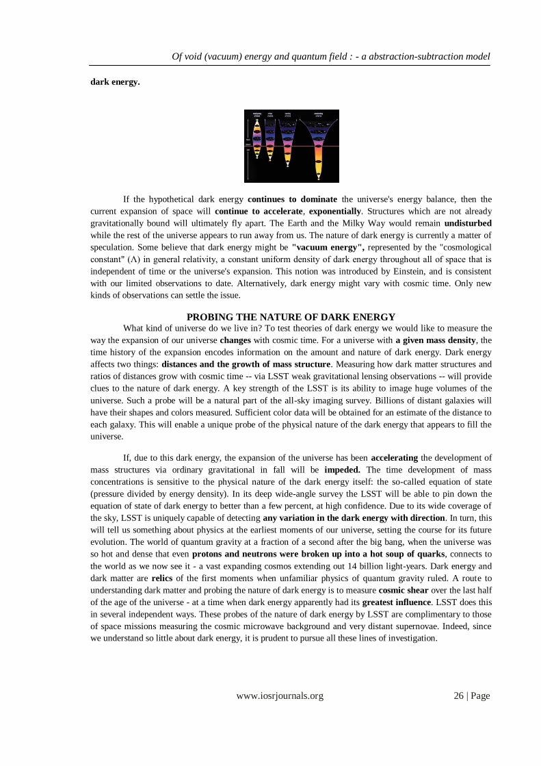
Of void (vacuum) energy and quantum field : - a abstraction-subtraction model

www.iosrjournals.org 26 | Page

dark energy.

If the hypothetical dark energy continues to dominate the universe's energy balance, then the

current expansion of space will continue to accelerate, exponentially. Structures which are not already

gravitationally bound will ultimately fly apart. The Earth and the Milky Way would remain undisturbed

while the rest of the universe appears to run away from us. The nature of dark energy is currently a matter of

speculation. Some believe that dark energy might be "vacuum energy", represented by the "cosmological

constant" (Λ) in general relativity, a constant uniform density of dark energy throughout all of space that is

independent of time or the universe's expansion. This notion was introduced by Einstein, and is consistent

with our limited observations to date. Alternatively, dark energy might vary with cosmic time. Only new

kinds of observations can settle the issue.

PROBING THE NATURE OF DARK ENERGY What kind of universe do we live in? To test theories of dark energy we would like to measure the

way the expansion of our universe changes with cosmic time. For a universe with a given mass density, the

time history of the expansion encodes information on the amount and nature of dark energy. Dark energy

affects two things: distances and the growth of mass structure. Measuring how dark matter structures and

ratios of distances grow with cosmic time -- via LSST weak gravitational lensing observations -- will provide

clues to the nature of dark energy. A key strength of the LSST is its ability to image huge volumes of the

universe. Such a probe will be a natural part of the all-sky imaging survey. Billions of distant galaxies will

have their shapes and colors measured. Sufficient color data will be obtained for an estimate of the distance to

each galaxy. This will enable a unique probe of the physical nature of the dark energy that appears to fill the

universe.

If, due to this dark energy, the expansion of the universe has been accelerating the development of

mass structures via ordinary gravitational in fall will be impeded. The time development of mass

concentrations is sensitive to the physical nature of the dark energy itself: the so-called equation of state

(pressure divided by energy density). In its deep wide-angle survey the LSST will be able to pin down the

equation of state of dark energy to better than a few percent, at high confidence. Due to its wide coverage of

the sky, LSST is uniquely capable of detecting any variation in the dark energy with direction. In turn, this

will tell us something about physics at the earliest moments of our universe, setting the course for its future

evolution. The world of quantum gravity at a fraction of a second after the big bang, when the universe was

so hot and dense that even protons and neutrons were broken up into a hot soup of quarks, connects to

the world as we now see it - a vast expanding cosmos extending out 14 billion light-years. Dark energy and

dark matter are relics of the first moments when unfamiliar physics of quantum gravity ruled. A route to

understanding dark matter and probing the nature of dark energy is to measure cosmic shear over the last half

of the age of the universe - at a time when dark energy apparently had its greatest influence. LSST does this

in several independent ways. These probes of the nature of dark energy by LSST are complimentary to those

of space missions measuring the cosmic microwave background and very distant supernovae. Indeed, since

we understand so little about dark energy, it is prudent to pursue all these lines of investigation.

Of void (vacuum) energy and quantum field : - a abstraction-subtraction model

www.iosrjournals.org 27 | Page

Splitting malleable fabric of Time from Space—Quantum Gravity and Vacuum Energy

A solar eclipse confirmed gravitational lensing and Einstein's concept of spacetime. But a new quantum

gravity theory now generating excitement separates time and space. Image: Photo Researchers, Inc.

Supplemental Material

Sidebar Splitting Time from Space The Evidence

It seems that unzipping the fabric of spacetime and harking back to 19th-century notions of time

could lead to a theory of quantum gravity.Physicists have struggled to marry quantum mechanics with

gravity for decades. In contrast, the other forces of nature have obediently fallen into line. For instance, the

electromagnetic force can be described quantum-mechanically by the motion of photons. Try and work out

the gravitational force between two objects in terms of a quantum graviton, however, and you quickly run

into trouble—the answer to every calculation is infinity. Some think it is about a matter of time. More

specifically, the problem is the way that time is tied up with space in Einstein‘s theory of gravity:

general relativity. Einstein famously overturned the Newtonian notion that time is absolute—steadily ticking

away in the background. Instead he argued that time is another dimension, woven together with space to form

a malleable fabric that is distorted by matter. The snag is that in quantum mechanics, time retains its

Newtonian aloofness, providing the stage against which matter dances but never being affected by its

presence. These two conceptions of time don‘t gel.

The solution many quantum gravity proponents and precursors is to snip threads that bind time to

space at very high energies, such as those found in the early universe where quantum gravity rules. ―I‘m

going back to Newton‘s idea that time and space is not equivalent,‖ HoYava says. At low energies, general

relativity emerges from this underlying framework, and the fabric of spacetime restitches. Many liken this

emergence to the way some exotic substances change phase. For instance, at low temperatures liquid

helium‘s properties change dramatically, becoming a ―super fluid‖ that can overcome friction. In fact, Ho

Yava has co-opted the mathematics of exotic phase transitions to build his theory of gravity. So far it seems to

be working: the infinities that plague other theories of quantum gravity have been tamed, and the theory

disgorges well-behaved graviton. It also seems to match with computer simulations of quantum gravity. In

particular, physicists have been checking if the model correctly describes the universe we see today. General

relativity scored a knockout blow when Einstein predicted the motion of Mercury with greater accuracy than

Newton‘s theory of gravity could.

Cosmic conundrums such as the singularity of the big bang, where the laws of physics break down,

can be explained by the theory of gravity. If HoYava gravity is true, argues cosmologist Robert

Brandenberger of McGill University in a paper published in the August Physical Review D, then the universe

didn‘t bang—it bounced. ―A universe filled with matter will contract down to a small—but finite—size

and then bounce out again, giving us the expanding cosmos we see today,‖ he says. Brandenberger

calculations show that ripples produced by the bounce match those already detected by satellites measuring

the cosmic microwave background, and he is now looking for signatures that could distinguish the bounce

from the big bang scenario.

Of void (vacuum) energy and quantum field : - a abstraction-subtraction model

www.iosrjournals.org 28 | Page

HoYava gravity may also create the ―illusion of dark matter,‖ says cosmologist Shinji Mukohyama

of Tokyo University. In the September Physical Review D, he explains that in certain circumstances

HoYava‘s graviton fluctuates as it interacts with normal matter, making gravity pull (INCREASE IN THE

GRAVITATIONAL FORCE)a bit more strongly than expected in general relativity. The effect could make

galaxies appear to contain more matter than can be seen. If that‘s not enough, cosmologist Mu-In Park of

Chonbuk National University in South Korea believes that HoYava gravity may also be behind the

accelerated expansion of the universe, currently attributed to a mysterious dark energy. One of the leading

explanations for its origin is that empty space contains some intrinsic energy that pushes (expands) the

universe outward. This intrinsic energy cannot be accounted for by general relativity but pops naturally out

of the equations of HoYava gravity, according to Park.

Casimir effect and vacuum energy fluctuations: Casimir forces on parallel plates

In quantum field theory, the Casimir effect and the Casimir–Polder force are physical forces arising

from a quantized field. The typical example is of two uncharged metallic plates in a vacuum,

like capacitors placed a few micrometers apart, without any external electromagnetic field. In

a classical description, the lack of an external field also means that there is no field between the plates, and no

force would be measured between them. When this field is instead studied using the QED

vacuum of quantum electrodynamics, it is seen that the plates do affect the virtual photons which constitute

the field, and generate a net force—either an attraction or a repulsion depending on the specific arrangement

of the two plates. Although the Casimir effect can be expressed in terms of virtual particles interacting with

the objects, it is best described and more easily calculated in terms of the zero-point energy of a quantized

field in the intervening space between the objects. This force has been measured, and is a striking example of

an effect purely due to second quantization However, the treatment of boundary conditions in these

calculations has led to some controversy. In fact "Casimir's original goal was to compute the van der Waals

force between polarizable molecules" of the metallic plates. Thus it can be interpreted without any reference

to the zero-point energy (vacuum energy) or virtual particles of quantum fields.

Because the strength of the force falls off rapidly with distance, it is only measurable when the distance

between the objects is extremely small. On a submicron scale, this force becomes so strong that it becomes

the dominant force between uncharged conductors. In fact, at separations of 10 nm—about 100 times the

typical size of an atom—the Casimir effect produces the equivalent of 1 atmosphere of pressure (101.325

kPa), the precise value depending on surface geometry and other factors. In modern theoretical physics, the

Casimir effect plays an important role in the chiral bag model of the nucleon; and in applied physics, it is

significant in some aspects of emerging micro technologies and nanotechnologies

The Casimir effect can be understood by the idea that the presence of conducting metals

and dielectrics alters the vacuum expectation value of the energy of the second quantized

electromagnetic Since the value of this energy depends on the shapes and positions of the conductors and

dielectrics, the Casimir effect makes itself manifest as a force between such objects.

VACUUM ENERGY The causes of the Casimir effect are described by quantum field theory, which states that all of the various

Of void (vacuum) energy and quantum field : - a abstraction-subtraction model

www.iosrjournals.org 29 | Page

fundamental fields, such as the electromagnetic, must be quantized at each and every point in space. In a

simplified view, a "field" in physics may be envisioned as if space were filled with interconnected vibrating

balls and springs, and the strength of the field can be visualized as the displacement of a ball from its rest

position. Vibrations in this field propagate and are governed by the appropriate wave equation for the

particular field in question. The second quantization of quantum field theory requires that each such ball-

spring combination be quantized, that is, that the strength of the field be quantized at each point in space. At

the most basic level, the field at each point in space is a simple harmonic oscillator, and its quantization

places a quantum harmonic oscillator at each point. Excitations of the field correspond to the elementary

particles of particle physics. However, even the vacuum has a vastly complex structure, so all calculations of

quantum field theory must be made in relation to this model of the vacuum.

The vacuum has, implicitly, all of the properties that a particle may have: spin, or polarization in the

case of light, energy, and so on. On average, most of these properties cancel out: the vacuum is, after all,

"empty" in this sense. One important exception is the vacuum energy or the vacuum expectation value of

the energy. The quantization of a simple harmonic oscillator states that the lowest possible energy orzero-

point energy that such an oscillator may have is

Summing over all possible oscillators at all points in space gives an infinite quantity. To remove this

infinity, one may argue that only differences in energy are physically measurable; this argument is the

underpinning of the theory of renormalization. In all practical calculations, this is how the infinity is always

handled. In a deeper sense, however, renormalization is unsatisfying, and the removal of this infinity presents

a challenge in the search for a Theory of Everything. Currently there is no compelling explanation for how

this infinity should be treated as essentially zero; a non-zero value is essentially the cosmological

constant and any large value causes trouble in cosmology.

Alternatively, a 2005 paper by Robert Jaffe of MIT states that "Casimir effects can be formulated

and Casimir forces can be computed without reference to zero point energies. They are relativistic,

quantum forces between charges and currents. The Casimir force (per unit area) between parallel plates

vanishes as alpha, the fine structure constant, goes to zero, and the standard result, which appears to be

independent of alpha, corresponds to the alpha → infinity limit," and that "The Casimir force is simply the

(relativistic, retarded) van der Waals force between the metal plates.

Casimir's observation was that the second-quantized quantum electromagnetic field, in the presence

of bulk bodies such as metals or dielectrics, must obey the same boundary conditions that the classical

electromagnetic field must obey. In particular, this affects the calculation of the vacuum energy in the

presence of a conductor or dielectric.

Consider, for example, the calculation of the vacuum expectation value of the electromagnetic

field inside a metal cavity, such as, for example, a radar cavity or a microwave waveguide. In this case, the

correct way to find the zero point energy of the field is to sum the energies of the standing waves of the

cavity. To each and every possible standing wave corresponds energy; say the energy of the nth standing

wave is . The vacuum expectation value of the energy of the electromagnetic field in the cavity is then

With the sum running over all possible values of n enumerating the standing waves. The factor of 1/2

corresponds to the fact that the zero-point energies are being summed (it is the same 1/2 as appears in the

equation ). Written in this way, this sum is clearly divergent; however, it can be used to

Of void (vacuum) energy and quantum field : - a abstraction-subtraction model

www.iosrjournals.org 30 | Page

create finite expressions.

In particular, one may ask how the zero point energy depends on the shape s of the cavity. Each

energy level depends on the shape, and so one should write for the energy level,

and for the vacuum expectation value. At this point comes an important observation: the force at

point p on the wall of the cavity is equal to the change in the vacuum energy if the shape s of the wall is

perturbed a little bit, say by , at point p. That is, one has

This value is finite in many practical calculations. Attraction between the plates can be easily

understood by focusing on the 1-dimensional situation. Suppose that a moveable conductive plate is

positioned at a short distance a from one of two widely separated plates (distance L apart). With a << L, the

states within the slot of width a are highly constrained so that the energy E of any one mode is widely

separated from that of the next. This is not the case in open region L, where there is a large number

(about L/a) of states with energy evenly spaced between E and the next mode in the narrow slot---in other

words, all slightly larger than E. Now on shortening a by da (< 0), the mode in the slot shrinks in wavelength

and therefore increases in energy proportional to -da/a, whereas all the outside L/a states lengthen and

correspondingly lower energy proportional to da/L (note the denominator). The net change is slightly

negative, because all the L/a modes' energies are slightly larger than the single mode in the slot.

Zeta-regularization-Vacuum energy as the sum of all excitation modes:

In the original calculation done by Casimir, he considered the space between a pair of conducting

metal plates at distance apart. In this case, the standing waves are particularly easy to calculate, since the

transverse component of the electric field and the normal component of the magnetic field must vanish on

the surface of a conductor. Assuming the parallel plates lie in the xy-plane, the standing waves are

Where stands for the electric component of the electromagnetic field, and, for brevity, the polarization and

the magnetic components are ignored here. Here, and are the wave vectors in directions parallel to

the plates, and

is the wave-vector perpendicular to the plates. Here, n is an integer, resulting from the requirement that ψ

vanish on the metal plates. The energy of this wave is

where c is the speed of light. The vacuum energy is then the sum over all possible excitation modes

Where A is the area of the metal plates, and a factor of 2 is introduced for the two possible polarizations of the

wave. This expression is clearly infinite, and to proceed with the calculation, it is convenient to introduce

a regulator the regulator will serve(EB) to make the expression finite, and in the end will be removed.

The zeta-regulated version of the energy per unit-area of the plate is

In the end, the limit is to be taken. Here s is just a complex number, not to be confused with the

Of void (vacuum) energy and quantum field : - a abstraction-subtraction model

www.iosrjournals.org 31 | Page

shape discussed previously. This integral/sum is finite for s real and larger than 3. The sum has a pole at s = 3,

but may be analytically continued to s = 0, where the expression is finite. The above expression is easily

simplified to:

Where polar coordinates were introduced to turn the double integral into a single

integral. The in front is the Jacobin, and the comes from the angular integration. The integral is easily

performed and converges if Re[s] > 3, resulting in

The sum clearly diverges at s in the neighborhood of zero, but if the damping of large-frequency excitations

corresponding to analytic continuation of the Riemann zeta function to s = 0 is assumed to make sense

physically in some way,

WORM HOLE AND VACUUM ENERGY

Exotic matter with negative energy density may be required to stabilize

a wormhole. Morris, Thorne and Yurtsever pointed out that the quantum mechanics of the Casimir effect can

be used to produce a locally mass-negative region of space-time and suggested that negative effect could be

used to stabilize a wormhole to allow faster than light travel.

In physics, a wormhole is a hypothetical topological feature of spacetime that would be, fundamentally, a

"shortcut" through spacetime. For a simple visual explanation of a wormhole, consider spacetime visualized

as a two-dimensional (2D) surface. If this surface is folded along a third dimension, it allows one to picture a

wormhole "bridge". (This is merely a visualization displayed to convey an essentially unvisualisable structure

existing in 4 or more dimensions. The parts of the wormhole could be higher-dimensional analogues for the

parts of the curved 2D surface; for example, instead of mouths which are circular holes in a 2D plane, a real

wormhole's mouths could be spheres in 3D space. A wormhole is, in theory, much like a tunnel with two

ends each in separate points in spacetime similar analysis can be used to explain Hawking radiation that

causes the slow "evaporation" of black holes (although this is generally visualized as the escape of one

particle from avirtual particle-antiparticle pair(PAIR LOSE), the other particle having been captured by the

black hole(GAINS).

AGE OF VACUUM ENERGY IN A RADIATION FILLED DESITTER UNIVERSE

So this is the de Sitter universe, and that it is also used as an approximation to inflationary models whose

dynamics are similar. Is this idea of "no beginning" sort of the basis for "eternal inflation? The only issue here is that any amount of matter or radiation causes the universe to have a finite age. So it is not considered

feasible for inflation to be past-eternal, because there will always be some matter or radiation, no matter

how diffuse

Inflation and Vacuum Energy Density-its effects on the classification of Vacuum energy: The "inflationary scenario", developed by Starobinsky and by Guth, offers a solution to the flatness-oldness

problem and the horizon problem. The inflationary scenario invokes a vacuum energy density. We normally

think of the vacuum as empty and massless, and we can determine that the density of the vacuum is less than

10-29 gm/cc now. But in quantum field theory, the vacuum is not empty, but rather filled with virtual particles

Of void (vacuum) energy and quantum field : - a abstraction-subtraction model

www.iosrjournals.org 32 | Page

The space-time diagram above shows virtual particle-antiparticle pairs forming out of nothing and

then annihilating back into nothing. For particles of mass m, one expects about one virtual particle in each

cubical volume with sides given by the Compton wavelength of the particle, h/mc, where h is Planck's

constant. Thus the expected density of the vacuum is rho = m4*c3/h3 which is rather large. For the largest

elementary particle mass usually considered, the Planck mass M defined by 2*pi*G*M2 = h*c, this density is

2*1091 gm/cc. That's a 2 followed by 91 zeroes! Thus the vacuum energy density is at least 120 orders of

magnitude smaller than the naive quantum estimate, so there must be a very effective suppression

mechanism at work. If a small residual vacuum energy density exists now, it leads to a "cosmological

constant" which is one proposed mechanism to relieve the tight squeeze between the Omega=1 model age of

the Universe, to = (2/3)/Ho = 9 Gyr, and the apparent age of the oldest globular clusters, 12-14 Gyr. The

vacuum energy density can do this because it produces a "repulsive gravity" that causes the expansion of the

Universe to accelerate instead of decelerate, and this increases to for a given Ho.

The inflationary scenario proposes that the vacuum energy was very large during a brief period

early in the history of the Universe. When the Universe is dominated by a vacuum energy density the scale

factor grows exponentially, a (t) = exp (H (t-to)). The Hubble constant really is constant during this epoch so

it doesn't need the "naught". If the inflationary epoch lasts long enough the exponential function gets very

large. This makes a (t) very large, and thus makes the radius of curvature of the Universe very large. The

diagram below shows our horizon superimposed on a very large radius sphere on top, or a smaller sphere on

the bottom. Since we can only see as far as our horizon, for the inflationary case on top the large radius sphere

looks almost flat to us. This is how Hawking also explains the connected and disconnected Euclidean

matrices.

This solves the ‗ flatness-oldness problem‘ as long as the ‗exponential growth during the inflationary epoch‘

continues for at least 100 doublings. Inflation also solves the horizon problem, because the future light cone

of an event that happens before inflation is expanded to a huge region by the growth during inflation.

Of void (vacuum) energy and quantum field : - a abstraction-subtraction model

www.iosrjournals.org 33 | Page

This space-time diagram shows the inflationary epoch tinted green, and the future light cones of two

events in red. The early event has a future light cone that covers a huge area that can easily encompass our

entire horizon. Thus we can explain why the temperature of the microwave background is so uniform

across the sky.

Large-Scale Structure and Anisotropy and Vacuum Energy. Of course the Universe is not really homogeneous, since it contains dense regions like galaxies and people.

Dense regions produce heterogeneity. These dense regions should affect the temperature of the microwave

background. Sachs and Wolfe (1967, ApJ, 147, 73) derived the effect of the gravitational potential

perturbations on the CMB. The gravitational potential, phi = -GM/r, will be negative in dense lumps, and

positive in less dense regions. Photons lose energy when they climb out of the gravitational potential wells of

the lumps:

This conformal space-time diagram above shows lumps as gray vertical bars, the epoch before

recombination as the hatched region, and the gravitational potential as the color-coded curve phi(x). Where

our past light cone intersects the surface of recombination, we see a temperature perturbed by dT/T =

phi/(3*c2). Sachs and Wolfe predicted temperature fluctuations dT/T as large as 1 percent, but we know now

that the Universe is far more homogeneous than Sachs and Wolfe thought. So observers worked for years to

get enough sensitivity to see the temperature differences around the sky. The first anisotropy to be detected

was the dipole anisotropy by Conklin in 1969: Part of the sky is hotter by (v/c)*to, while the blue part of the

sky is colder by (v/c)*to, where the inferred velocity is v = 368 km/sec. This is how we measure the

velocity of the Solar System relative to the observable Universe. It was another 23 years before

the anisotropy predicted by Sachs and Wolfe was detected by Smoot et al. (1992, ApJL, 396, 1). The

amplitude was 1 part in 100,000 instead of 1 part in 100, but was perfectly consistent with Lambda-

CDM [Wright et al. 1992, ApJL, 396, 13].

Cosmic anisotropy and Void: Cosmic anisotropy (and detector noise) after the dipole pattern and the radiation from the Milky

Way have been subtracted out. The anisotropy if converted into a gravitational potential using Sachs and

Wolfe's result and that potential is then expressed as a height assuming a constant acceleration of gravity

equal to the gravity on the Earth, we get a height of twice the distance from the Earth to the Sun. The

"mountains and valleys" of the Universe are really quite large. Inflation predicts a certain statistical pattern in

the anisotropy. The quantum fluctuations normally affect very small regions of space, but the huge

exponential expansion during the inflationary epoch makes these tiny regions observable. The pattern

formed by adding all of the effects from events of all ages is known as "equal power on all scales", and it

agrees with the COBE data. Having found that the observed pattern of anisotropy is consistent with inflation,

we can also ask whether the amplitude implies gravitational forces large enough to produce the observed

clustering of galaxies. The conformal space-time diagram above shows the phi(x) at recombination

determined by COBE's dT data, and the worldliness of galaxies which are perturbed by the gravitational

forces produced by the gradient of the potential. Matter flows "downhill" away from peaks of the potential

Of void (vacuum) energy and quantum field : - a abstraction-subtraction model

www.iosrjournals.org 34 | Page

producing voids in the current distribution of galaxies, while valleys in the potential (blue spots) are

where the clusters of galaxies form.

ENERGY DENSITY IN THE UNIVERSE IS VACUUM DENSITY

Gravitational forces are large enough to produce the observed clustering, but only if these forces are

not opposed by other forces. If the all the matter in the Universe is made out of the ordinary chemical

elements, then there was a very effective opposing force before recombination, because the free electrons

which are now bound into atoms were very effective at scattering the photons of the cosmic background. We

can therefore conclude that most of the matter in the Universe is "dark matter" that does not emit,

absorb or scatter light. Furthermore, observations of distant supernovae have shown that most of the energy

density of the Universe is a vacuum energy density (a "dark energy") like Einstein's cosmological constant that causes an accelerating expansion of the Universe. These strange conclusions have been greatly

strengthened by temperature anisotropy data at smaller angular scales which was provided by the Wilkinson

Microwave Anisotropy Probe (WMAP) in 2003.

Pressure less matter ( R-3), radiation ( R-4

) and vacuum energy

The equation of motion for the scale factor can be obtained in a quasi-Newtonian fashion. Consider a sphere

about some arbitrary point, and let the radius be R (t) r, where r is arbitrary. The motion of a point at the edge

of the sphere will, in Newtonian gravity, be influenced only by the interior mass. We can therefore write

down immediately a differential equationFriedmann's equation) that expresses conservation of energy: r)

2 / 2 - GM / (Rr) = constant. In fact, to get this far, we do require general relativity: the gravitation from mass

shells at large distances is not Newtonian, and so we cannot employ the usual argument about their effect

being zero. In fact, the result that the gravitational field inside a uniform shell is zero does hold in general

relativity, and is known as Birkhoff's theorem . General relativity becomes even more vital in giving us the

constant of integration in Friedman‘s equation The Friedman equation shows that a universe that is spatially

closed (with k = +1) has negative total ``energy'': the expansion will eventually be halted by gravity, and the universe will recollapse. Conversely, an unbound model is spatially open (k = -1) and will expand

forever. This is marvelously simple: the dynamics of the entire universe are the same as those of a cannonball

fired vertically against the Earth's gravity. Just as the Earth's gravity defines an escape velocity for projectiles,

so a universe that expands sufficiently fast will continue to expand forever. Conversely, for a given rate of

expansion there is a critical density that will bring the expansion asymptotically to a halt

This connection between the rate of expansion of the universe and its global geometry is deep result. An

alternative line of attack is to rewrite the Friedmann equation in terms of the Hubble parameter:

The ``flat'' universe with k = 0 arises for a particular critical density. We are therefore led to define a density

parameter as the ratio of density to critical density:

Since and H change with time, this defines an epoch-dependent density parameter. The current value of the

parameter should strictly be denoted by 0.Pressureless matter ( R-3), radiation ( R-4

) and

vacuum energy ( constant Note that the transformations and transactions take place continuously

Of void (vacuum) energy and quantum field : - a abstraction-subtraction model

www.iosrjournals.org 35 | Page

depite the constant state of the Vacuum energy).is what universe could be divided in to. The first two

relations just say that the number density of particles is diluted by the expansion, with photons also having

their energy reduced by the redshift; the third relation applies for Einstein's cosmological constant. The

Hubble constant thus sets the curvature length, which becomes infinitely large as approaches unity from

either direction. Only in the limit of zero density does this length become equal to the other common measure

of the size of the universe - the Hubble length, c / H0.t2/3.

One of the great conclusions of relativistic cosmology: the universe is of finite age, and had its

origin in a mathematical singularity at which the scale factor went to zero, leading to a divergent spacetime

curvature. Since zero scale factor also implies infinite density (and temperature), the inferred(manifested)

picture of the early universe is one of unimaginable violence tempestuous and turbulent internal

differentiation and comparative variability and structural morphology and within normative aspect of

expectations usually drawn by cosmologists. The term big bang was coined by Fred Hoyle to describe this

beginning, although it was intended somewhat critically. The problem with the singularity is that it marks the

breakdown of the laws of physics; we cannot extrapolate the solution for R (t) to t < 0, and so the origin of

the expansion becomes an unexplained boundary condition

MASS DENSITY AND VACUUM ENERGY -THE REPULSIVE COUNTERBALANCING FORCE:

Since = -p for vacuum energy, and this is the only source of pressure if we ignore radiation, this tells us

that = 3 and hence that the mass density is twice the vacuum density. The total density is hence positive

and k = 1; we have a closed model. Notice that what this says is that a positive vacuum energy acts in a

repulsive way, balancing the attraction of normal matter. This is related to the idea of + 3p as the effective

source density for gravity. This insight alone should make one appreciate that the static model cannot be

stable: if we perturb the scale factor by a small positive amount, the vacuum repulsion is unchanged

whereas the ``normal'' gravitational attraction is reduced, so that the model will tend to expand further (or

contract, if the initial perturbation was negative). Thinking along these lines, a tidy history of science would

have required Einstein to predict the expanding universe in advance of its observation.

VACUUM ENERGY AND DESITTER SPACE:. DE SITTER SPACE Before going on to the general case, it is worth looking at the endpoint of an

outwards perturbation of Einstein's static model, first studied by de Sitter and named after him. This universe

is completely dominated by vacuum energy, and is clearly the limit of the unstable expansion, since the

density of matter redshift to zero while the vacuum energy remains constant. It was thought that the cosmological constant is what caused the expansion. He tells us that the Hubble constant really is constant,

and so the model necessarily has exponential expansion, R exp(Ht), exactly as for de Sitter space.

Furthermore, it is necessary that k = 0, as may be seen by considering the transverse part of the Robertson-

Walker metric: d 2 = [R (t) Sk (r) d ]

2. This has the convention that r is a dimensionless commoving

coordinate; if we divide by R0 and change to physical radius r', the metric becomes d 2 = [a (t) R0 Sk (r' /

R0) d ]2. The current scale factor R0 now plays the role of a curvature length, determining the distance over

which the model is spatially Euclidean. However, any such curvature radius must be constant in the steady-

state model, so the only possibility is that it is infinite and that k = 0. We thus see that de Sitter space is a

steady-state universe: it contains a constant vacuum energy density, and has an infinite age, lacking any

big-bang singularity. In this sense, some aspects of the steady-state model have been resurrected in

inflationary cosmology. However, de Sitter space is a rather uninteresting model because it contains no

matter. Introducing matter into a steady-state universe violates energy conservation, since matter does not

have the p = - c2 equation of state that allows the density to remain constant. This is the most radical aspect

of steady-state models: they require continuous creation of matter. (Carroll, Press & Turner 1992

If the density is below the critical density, the result would be that the universe will expand forever, at an

ever decreasing rate; the universe will be open. In this case its global geometry will have negative curvature,

like the surface of a trumpet. The angles of a large triangle add up to less that 180o.If the density is exactly

equal to the critical density the universe will have a flat geometry, and universe will expand forever at an

ever decreasing rate. The angles of all triangles add up to 180o.

Of void (vacuum) energy and quantum field : - a abstraction-subtraction model

www.iosrjournals.org 36 | Page

STABILITY ANALYSIS:

From the above stability analysis we infer the following:

1. The adjustment process is stable in the sense that the system of oxygen consumption converges to

equilibrium.

2.The approach to equilibrium is a steady one , and there exists progressively diminishing oscillations around

the equilibrium point

3.Conditions 4 and 2 are independent of the size and direction of initial disturbance

4.The actual shape of the time path of VE is determined by efficiency parameter , the strength of the response

of the portfolio in question, and the initial disturbance5.Result 3 warns us that we need to make an exhaustive

study of the behavior of any case in which generalization derived from the model do not hold

6.Growth studies as the one in the extant context are related to the systemic growth paths with full

employment of resources that are available in question, in the present case terrestrial organisms –oxygen

consumption-dead organic matter and decomposer organisms

7. Some authors were interested in such questions, whether growing system could produce full employment

of all factors, whether or not there was a full employment natural rate growth path and perpetual oscillations

around it. It is to be noted some systems pose extremely difficult stability problems. As an instance, one can

quote example of pockets of PRIGOGINE‘S DISSIPATIVE STRCTURES like open cells and drizzle in

complex networks in marine stratocumulus. Other examples are clustering and synchronization of lightning

flashes adjunct to thunderstorms, coupled studies of microphysics and aqueous chemistry.

QUANTUM FIELD(QF) PORTFOLIO::

Assumptions:

(1)Category 1 is representative of QF vis-à-vis VE category 1

(2)Category 2 constitutes QF in correspondence with the similar classification of QF(3) Category 3 of QF

with respect to category 3 of VE

(a)The speed of growth of QF category 1 is a linear function of that sector in category 2 at the time of

reckoning. As before the accentuation coefficient that characterizes the speed of growth in category 1 is the

proportionality factor between balance in category 1 and category 2.

(b)The dissipation coefficient in the growth model is attributable to two factors;(1) With the progress of time

terrestrial organism sector gets aged and become eligible for transfer to the next category. Notwithstanding

Category 3 does not have such a provision for further transference provisionalities

©Inflow into category 2 is only from category 1 in the form of transfer of balance of QF from the category

1.This is evident from the age wise classification scheme. As a result, the speed of growth of category 2 is

dependent upon the amount of inflow, which is a function of the quantum of balance of terrestrial organism

sector under the category 1.The balance of QF sector in category 3 is because of transfer of balance from

category 2. It is dependent on the amount of QF (See above discussion of energy density of matter both in

classical and quantum mechanics) sector under category 2.

Of void (vacuum) energy and quantum field : - a abstraction-subtraction model

www.iosrjournals.org 37 | Page

NOTATION :

𝑇24 : Balance standing in the category 1 of QF

𝑇25 : Balance standing in the category 2 of QF

𝑇26 : Balance standing in the category 3 of QF

𝑏24 4 , 𝑏25

4 , 𝑏26 4 : Accentuation coefficients

𝑏24′ 4 , 𝑏25

′ 4 , 𝑏26′ 4 : Dissipation coefficients

FORMULATION OF THE SYSTEM : Under the above assumptions, we derive the following :

a) The growth speed in category 1 is the sum of two parts:

1. A term + 𝑏24 4 𝑇25 proportional to the amount of balance of the category 2

2. A term – 𝑏24′ 4 𝑇24 representing the quantum of balance dissipated from category 1 .

b) The growth speed in category 2 is the sum of two parts:

1. A term + 𝑏25 4 𝑇24 constitutive of the amount of inflow from the category

2. A term – 𝑏25′ 4 𝑇25 the dissipation factor

The growth speed under category 3 is attributable to inflow from category 2 and any other dissipations in QF

GOVERNING EQUATIONS: Following are the differential equations that govern the growth in the terrestrial organisms portfolio

𝑑𝑇24

𝑑𝑡= 𝑏24

4 𝑇25 − 𝑏24′ 4 𝑇24

12

𝑑𝑇25

𝑑𝑡= 𝑏25

4 𝑇24 − 𝑏25′ 4 𝑇25

13

𝑑𝑇26

𝑑𝑡= 𝑏26

4 𝑇25 − 𝑏26′ 4 𝑇26

14

𝑏𝑖 4 > 0 , 𝑖 = 24,25,26 15

𝑏𝑖′ 4 > 0 , 𝑖 = 24,25,26 16

𝑏25 4 < 𝑏24

′ 4 17

𝑏26 4 < 𝑏25

′ 4 18

Following the same procedure outlined in the previous section , the general solution of the governing

equations is 𝛼𝑖′𝑇𝑖 + 𝛽𝑖

′𝑇𝑖 + 𝛾𝑖′𝑇𝑖 = 𝐶𝑖

′𝑒𝑖𝜆′

𝑖𝑡 , 𝑖 = 24,25,26 where 𝐶24′ ,𝐶25

′ ,𝐶26′ are arbitrary constant

coefficients and 𝛼24′ ,𝛼25

′ ,𝛼26′ ,𝛾24

′ , 𝛾25′ ,𝛾26

′ corresponding multipliers to the characteristic roots of the

system

VACUUM ENERGY(VE) AND QUANTUM FIELD(QF) SYSTEM-INTERPRETATION OF

DUAL SYSTEM

Of void (vacuum) energy and quantum field : - a abstraction-subtraction model

www.iosrjournals.org 38 | Page

We will denote

1) By 𝑇𝑖 𝑡 , 𝑖 = 24,25,26 , the three parts of the QF analogously to the 𝐺𝑖 of the VE

2) 𝑎𝑖′′ 4 𝑇25 , 𝑡 (𝑇25 ≥ 0, 𝑡 ≥ 0) ,the contribution of the QF to the dissipation coefficient of the VE

3) By −𝑏𝑖′′ 4 𝐺24 , 𝐺25 ,𝐺26 , 𝑡 = − 𝑏𝑖

′′ 4 𝐺27 , 𝑡 , the contribution of the VE to the dissipation

coefficient of the QF

GOVERNING EQUATIONS: The differential system of this model is now

𝑑𝐺24

𝑑𝑡= 𝑎24

4 𝐺25 − 𝑎24′ 4 + 𝑎24

′′ 4 𝑇25 , 𝑡 𝐺24 19

𝑑𝐺25

𝑑𝑡= 𝑎25

4 𝐺24 − 𝑎25′ 4 + 𝑎25

′′ 4 𝑇25 , 𝑡 𝐺25 20

𝑑𝐺26

𝑑𝑡= 𝑎26

4 𝐺25 − 𝑎26′ 4 + 𝑎26

′′ 4 𝑇25 , 𝑡 𝐺26 21

𝑑𝑇24

𝑑𝑡= 𝑏24

4 𝑇25 − 𝑏24′ 4 − 𝑏24

′′ 4 𝐺27 , 𝑡 𝑇24 22

𝑑𝑇25

𝑑𝑡= 𝑏25

4 𝑇24 − 𝑏25′ 4 − 𝑏25

′′ 4 𝐺27 , 𝑡 𝑇25 23

𝑑𝑇26

𝑑𝑡= 𝑏26

4 𝑇25 − 𝑏26′ 4 − 𝑏26

′′ 4 𝐺27 , 𝑡 𝑇26 24

+ 𝑎24′′ 4 𝑇25 , 𝑡 = First augmentation factor DUE TO QF

− 𝑏24′′ 4 𝐺, 𝑡 = First detritions factor contributed by VE to the dissipation of QF

Where we suppose

𝑎𝑖 4 , 𝑎𝑖

′ 4 , 𝑎𝑖′′ 4 , 𝑏𝑖

4 , 𝑏𝑖′ 4 , 𝑏𝑖

′′ 4 > 0, 𝑖, 𝑗 = 24,25,26

(A) The functions 𝑎𝑖′′ 4 , 𝑏𝑖

′′ 4 are positive continuous increasing and bounded.

Definition of (𝑝𝑖) 4 , (𝑟𝑖)

4 :

𝑎𝑖′′ 4 (𝑇25 , 𝑡) ≤ (𝑝𝑖)

4 ≤ ( 𝐴 24 )(4)

𝑏𝑖′′ 4 ( 𝐺27 , 𝑡) ≤ (𝑟𝑖)

4 ≤ (𝑏𝑖′) 4 ≤ ( 𝐵 24 )(4)

25

26

(B) 𝑙𝑖𝑚𝑇2→∞ 𝑎𝑖′′ 4 𝑇25 , 𝑡 = (𝑝𝑖)

4

limG→∞

𝑏𝑖′′ 4 𝐺27 , 𝑡 = (𝑟𝑖)

4

Definition of ( 𝐴 24 )(4), ( 𝐵 24 )(4) :

Where ( 𝐴 24 )(4), ( 𝐵 24 )(4), (𝑝𝑖) 4 , (𝑟𝑖)

4 are positive constants and 𝑖 = 24,25,26

27

28

Of void (vacuum) energy and quantum field : - a abstraction-subtraction model

www.iosrjournals.org 39 | Page

They satisfy Lipschitz condition:

|(𝑎𝑖′′ ) 4 𝑇25

′ , 𝑡 − (𝑎𝑖′′ ) 4 𝑇25 , 𝑡 | ≤ ( 𝑘 24 )(4)|𝑇25 − 𝑇25

′ |𝑒−( 𝑀 24 )(4)𝑡

|(𝑏𝑖′′ ) 4 𝐺27

′ , 𝑡 − (𝑏𝑖′′ ) 4 𝐺27 ,𝑇 | < ( 𝑘 24 )(4)|| 𝐺27 − 𝐺27

′ ||𝑒−( 𝑀 24 )(4)𝑡

29

30

With the Lipschitz condition, we place a restriction on the behavior of functions (𝑎𝑖′′ ) 4 𝑇25

′ , 𝑡

and(𝑎𝑖′′ ) 4 𝑇25 , 𝑡 𝑇25

′ , 𝑡 And 𝑇25 , 𝑡 are points belonging to the interval ( 𝑘 24 )(4), ( 𝑀 24 )(4) . It

is to be noted that (𝑎𝑖′′ ) 4 𝑇25 , 𝑡 is uniformly continuous. In the eventuality of the fact, that if

( 𝑀 24 )(4) = 4 then the function (𝑎𝑖′′ ) 4 𝑇25 , 𝑡 , the first augmentation coefficient, would be

absolutely continuous.

Definition of ( 𝑀 24 )(4), ( 𝑘 24 )(4) :

( 𝑀 24 )(4), ( 𝑘 24 )(4), are positive constants

(𝑎𝑖) 4

( 𝑀 24 )(4) ,

(𝑏𝑖) 4

( 𝑀 24 )(4)< 1

31

Definition of ( 𝑃 24 )(4), ( 𝑄 24 )(4) :

(C) There exists two constants ( 𝑃 24 )(4) and ( 𝑄 24 )(4) which together with

( 𝑀 24 )(4), ( 𝑘 24 )(4), (𝐴 24 )(4)𝑎𝑛𝑑 ( 𝐵 24 )(4) and the constants

(𝑎𝑖) 4 , (𝑎𝑖

′ ) 4 , (𝑏𝑖) 4 , (𝑏𝑖

′) 4 , (𝑝𝑖) 4 , (𝑟𝑖)

4 , 𝑖 = 24,25,26,

satisfy the inequalities

1

( 𝑀 24 )(4)[ (𝑎𝑖)

4 + (𝑎𝑖′ ) 4 + ( 𝐴 24 )(4) + ( 𝑃 24 )(4) ( 𝑘 24 )(4)] < 1

1

( 𝑀 24 )(4)[ (𝑏𝑖)

4 + (𝑏𝑖′) 4 + ( 𝐵 24 )(4) + ( 𝑄 24 )(4) ( 𝑘 24 )(4)] < 1

32

33

Theorem 4: if the conditions (A)-(E) above are fulfilled, there exists a solution satisfying the

conditions

Definition of 𝐺𝑖 0 , 𝑇𝑖 0 :

𝐺𝑖 𝑡 ≤ 𝑃 24 4

𝑒 𝑀 24 4 𝑡 , 𝐺𝑖 0 = 𝐺𝑖0 > 0

𝑇𝑖(𝑡) ≤ ( 𝑄 24 )(4)𝑒( 𝑀 24 )(4)𝑡 , 𝑇𝑖 0 = 𝑇𝑖0 > 0

Proof:

Consider operator 𝒜(4) defined on the space of sextuples of continuous functions 𝐺𝑖 , 𝑇𝑖 : ℝ+ → ℝ+

which satisfy

𝐺𝑖 0 = 𝐺𝑖0 , 𝑇𝑖 0 = 𝑇𝑖

0 , 𝐺𝑖0 ≤ ( 𝑃 24 )(4) ,𝑇𝑖

0 ≤ ( 𝑄 24 )(4), 34

Of void (vacuum) energy and quantum field : - a abstraction-subtraction model

www.iosrjournals.org 40 | Page

0 ≤ 𝐺𝑖 𝑡 − 𝐺𝑖0 ≤ ( 𝑃 24 )(4)𝑒( 𝑀 24 )(4)𝑡 35

0 ≤ 𝑇𝑖 𝑡 − 𝑇𝑖0 ≤ ( 𝑄 24 )(4)𝑒( 𝑀 24 )(4)𝑡 36

By

𝐺 24 𝑡 = 𝐺240 + (𝑎24 ) 4 𝐺25 𝑠 24 − (𝑎24

′ ) 4 + 𝑎24′′ ) 4 𝑇25 𝑠 24 , 𝑠 24 𝐺24 𝑠 24 𝑑𝑠 24

𝑡

0

37

𝐺 25 𝑡 = 𝐺250 + (𝑎25 ) 4 𝐺24 𝑠 24 − (𝑎25

′ ) 4 + (𝑎25′′ ) 4 𝑇25 𝑠 24 , 𝑠 24 𝐺25 𝑠 24 𝑑𝑠 24

𝑡

0

38

𝐺 26 𝑡 = 𝐺260 + (𝑎26 ) 4 𝐺25 𝑠 24 − (𝑎26

′ ) 4 + (𝑎26′′ ) 4 𝑇25 𝑠 24 , 𝑠 24 𝐺26 𝑠 24 𝑑𝑠 24

𝑡

0 39

𝑇 24 𝑡 = 𝑇240 + (𝑏24 ) 4 𝑇25 𝑠 24 − (𝑏24

′ ) 4 − (𝑏24′′ ) 4 𝐺 𝑠 24 , 𝑠 24 𝑇24 𝑠 24 𝑑𝑠 24

𝑡

0

40

𝑇 25 𝑡 = 𝑇250 + (𝑏25 ) 4 𝑇24 𝑠 24 − (𝑏25

′ ) 4 − (𝑏25′′ ) 4 𝐺 𝑠 24 , 𝑠 24 𝑇25 𝑠 24 𝑑𝑠 24

𝑡

0

41

T 26 t = T260 + (𝑏26 ) 4 𝑇25 𝑠 24 − (𝑏26

′ ) 4 − (𝑏26′′ ) 4 𝐺 𝑠 24 , 𝑠 24 𝑇26 𝑠 24 𝑑𝑠 24

𝑡

0

Where 𝑠 24 is the integrand that is integrated over an interval 0, 𝑡

42

(a) The operator 𝒜(4) maps the space of functions satisfying 34,35,36 into itself .Indeed it is obvious

that

𝐺24 𝑡 ≤ 𝐺240 + (𝑎24 ) 4 𝐺25

0 +( 𝑃 24 )(4)𝑒( 𝑀 24 )(4)𝑠 24

𝑡

0

𝑑𝑠 24 =

1 + (𝑎24 ) 4 𝑡 𝐺250 +

(𝑎24 ) 4 ( 𝑃 24 )(4)

( 𝑀 24 )(4) 𝑒( 𝑀 24 )(4)𝑡 − 1

43

From which it follows that

𝐺24 𝑡 − 𝐺240 𝑒−( 𝑀 24 )(4)𝑡 ≤

(𝑎24 ) 4

( 𝑀 24 )(4) ( 𝑃 24 )(4) + 𝐺25

0 𝑒 −

( 𝑃 24 )(4)+𝐺250

𝐺250

+ ( 𝑃 24 )(4)

𝐺𝑖0 is as defined in the statement of theorem 1

44

Analogous inequalities hold also for 𝐺25 ,𝐺26 ,𝑇24 ,𝑇25 , 𝑇26

It is now sufficient to take (𝑎𝑖) 4

( 𝑀 24 )(4) ,(𝑏𝑖) 4

( 𝑀 24 )(4) < 1 and to choose

( P 24 )(4) and ( Q 24 )(4) large to have

Of void (vacuum) energy and quantum field : - a abstraction-subtraction model

www.iosrjournals.org 41 | Page

(𝑎𝑖) 4

(𝑀 24 ) 4 ( 𝑃 24 ) 4 + ( 𝑃 24 )(4) + 𝐺𝑗

0 𝑒−

( 𝑃 24 )(4)+𝐺𝑗0

𝐺𝑗0

≤ ( 𝑃 24 )(4)

45

(𝑏𝑖) 4

(𝑀 24) 4 ( 𝑄 24 )(4) + 𝑇𝑗

0 𝑒−

( 𝑄 24 )(4)+𝑇𝑗0

𝑇𝑗0

+ ( 𝑄 24 )(4) ≤ ( 𝑄 24 )(4)

46

In order that the operator 𝒜(4) transforms the space of sextuples of functions 𝐺𝑖 ,𝑇𝑖 satisfying 34,35,36

into itself

The operator 𝒜(4) is a contraction with respect to the metric

𝑑 𝐺27 1 , 𝑇27

1 , 𝐺27 2 , 𝑇27

2 =

𝑠𝑢𝑝𝑖

{𝑚𝑎𝑥𝑡∈ℝ+

𝐺𝑖 1

𝑡 − 𝐺𝑖 2

𝑡 𝑒−(𝑀 24 ) 4 𝑡 ,𝑚𝑎𝑥𝑡∈ℝ+

𝑇𝑖 1

𝑡 − 𝑇𝑖 2

𝑡 𝑒−(𝑀 24 ) 4 𝑡}

Indeed if we denote

Definition of 𝐺27 , 𝑇27 : 𝐺27 , 𝑇27 = 𝒜(4)( 𝐺27 , 𝑇27 )

It results

𝐺 24 1

− 𝐺 𝑖 2

≤ (𝑎24 ) 4

𝑡

0

𝐺25 1

− 𝐺25 2

𝑒−( 𝑀 24 ) 4 𝑠 24 𝑒( 𝑀 24 ) 4 𝑠 24 𝑑𝑠 24 +

{(𝑎24′ ) 4 𝐺24

1 − 𝐺24

2 𝑒−( 𝑀 24 ) 4 𝑠 24 𝑒−( 𝑀 24 ) 4 𝑠 24

𝑡

0

+

(𝑎24′′ ) 4 𝑇25

1 , 𝑠 24 𝐺24

1 − 𝐺24

2 𝑒−( 𝑀 24 ) 4 𝑠 24 𝑒( 𝑀 24 ) 4 𝑠 24 +

𝐺24 2

|(𝑎24′′ ) 4 𝑇25

4 , 𝑠 24 − (𝑎24

′′ ) 4 𝑇25 2

, 𝑠 24 | 𝑒−( 𝑀 24 ) 4 𝑠 24 𝑒( 𝑀 24 ) 4 𝑠 24 }𝑑𝑠 24

Where 𝑠 24 represents integrand that is integrated over the interval 0, t

From the hypotheses on 25,26,27,28 and 29 it follows

47

48

49

𝐺27 1 − 𝐺27

2 𝑒−( 𝑀 24 ) 4 𝑡

≤1

( 𝑀 24) 4 (𝑎24 ) 4 + (𝑎24

′ ) 4 + ( 𝐴 24 ) 4

+ ( 𝑃 24 ) 4 ( 𝑘 24 ) 4 𝑑 𝐺27 1 , 𝑇27

1 ; 𝐺27 2 , 𝑇27

2

And analogous inequalities for 𝐺𝑖 𝑎𝑛𝑑 𝑇𝑖 . Taking into account the hypothesis (34,35,36) the result

follows

50

Remark 4: The fact that we supposed (𝑎24′′ ) 4 and (𝑏24

′′ ) 4 depending also on t can be considered as

not conformal with the reality, however we have put this hypothesis ,in order that we can postulate

condition necessary to prove the uniqueness of the solution bounded by

( 𝑃 24 ) 4 𝑒( 𝑀 24 ) 4 𝑡 𝑎𝑛𝑑 ( 𝑄 24 ) 4 𝑒( 𝑀 24 ) 4 𝑡 respectively of ℝ+.

51

Of void (vacuum) energy and quantum field : - a abstraction-subtraction model

www.iosrjournals.org 42 | Page

If instead of proving the existence of the solution on ℝ+, we have to prove it only on a compact then it

suffices to consider that (𝑎𝑖′′ ) 4 and (𝑏𝑖

′′ ) 4 , 𝑖 = 24,25,26 depend only on T25 and respectively on

𝐺27 (𝑎𝑛𝑑 𝑛𝑜𝑡 𝑜𝑛 𝑡) and hypothesis can replaced by a usual Lipschitz condition.

Remark 2: There does not exist any 𝑡 where 𝐺𝑖 𝑡 = 0 𝑎𝑛𝑑 𝑇𝑖 𝑡 = 0

From 19 to 24 it results

𝐺𝑖 𝑡 ≥ 𝐺𝑖0𝑒 − (𝑎𝑖

′ ) 4 −(𝑎𝑖′′ ) 4 𝑇25 𝑠 24 ,𝑠 24 𝑑𝑠 24

𝑡0 ≥ 0

𝑇𝑖 𝑡 ≥ 𝑇𝑖0𝑒 −(𝑏𝑖

′ ) 4 𝑡 > 0 for t > 0

52

Definition of ( 𝑀 24 ) 4 1, ( 𝑀 24) 4

2 𝑎𝑛𝑑 ( 𝑀 24) 4

3 :

Remark 3: if 𝐺24 is bounded, the same property have also 𝐺25 𝑎𝑛𝑑 𝐺26 . indeed if

𝐺24 < ( 𝑀 24 ) 4 it follows 𝑑𝐺25

𝑑𝑡≤ ( 𝑀 24) 4

1− (𝑎25

′ ) 4 𝐺25 and by integrating

𝐺25 ≤ ( 𝑀 24) 4 2

= 𝐺250 + 2(𝑎25 ) 4 ( 𝑀 24 ) 4

1/(𝑎25

′ ) 4

In the same way , one can obtain

𝐺26 ≤ ( 𝑀 24 ) 4 3

= 𝐺260 + 2(𝑎26 ) 4 ( 𝑀 24 ) 4

2/(𝑎26

′ ) 4

If 𝐺25 𝑜𝑟 𝐺26 is bounded, the same property follows for 𝐺24 , 𝐺26 and 𝐺24 , 𝐺25 respectively.

53

Remark 4: If 𝐺24 𝑖𝑠 bounded, from below, the same property holds for 𝐺25 𝑎𝑛𝑑 𝐺26 . The proof is

analogous with the preceding one. An analogous property is true if 𝐺25 is bounded from below.

54

Remark 5: If T24 is bounded from below and lim𝑡→∞((𝑏𝑖′′ ) 4 ( 𝐺27 𝑡 , 𝑡)) = (𝑏25

′ ) 4 then 𝑇25 →

∞.

Definition of 𝑚 4 and 𝜀4 :

Indeed let 𝑡4 be so that for 𝑡 > 𝑡4

(𝑏25 ) 4 − (𝑏𝑖′′ ) 4 ( 𝐺27 𝑡 , 𝑡) < 𝜀4 ,𝑇24 (𝑡) > 𝑚 4

55

Then 𝑑𝑇25

𝑑𝑡≥ (𝑎25 ) 4 𝑚 4 − 𝜀4𝑇25 which leads to

𝑇25 ≥ (𝑎25 ) 4 𝑚 4

𝜀4 1 − 𝑒−𝜀4𝑡 + 𝑇25

0 𝑒−𝜀4𝑡 If we take t such that 𝑒−𝜀4𝑡 = 1

2 it results

𝑇25 ≥ (𝑎25 ) 4 𝑚 4

2 , 𝑡 = 𝑙𝑜𝑔

2

𝜀4 By taking now 𝜀4 sufficiently small one sees that T25 is

unbounded. The same property holds for 𝑇26 if lim𝑡→∞(𝑏26′′ ) 4 𝐺27 𝑡 , 𝑡 = (𝑏26

′ ) 4

We now state a more precise theorem about the behaviors at infinity of the solutions of equations 37 to

42

Behavior of the solutions of equation 37 to 12

Theorem 2: If we denote and define

Of void (vacuum) energy and quantum field : - a abstraction-subtraction model

www.iosrjournals.org 43 | Page

Definition of (𝜎1) 4 , (𝜎2) 4 , (𝜏1) 4 , (𝜏2) 4 :

(a) (𝜎1) 4 , (𝜎2) 4 , (𝜏1) 4 , (𝜏2) 4 four constants satisfying

−(𝜎2) 4 ≤ −(𝑎24′ ) 4 + (𝑎25

′ ) 4 − (𝑎24′′ ) 4 𝑇25 , 𝑡 + (𝑎25

′′ ) 4 𝑇25 , 𝑡 ≤ −(𝜎1) 4

−(𝜏2) 4 ≤ −(𝑏24′ ) 4 + (𝑏25

′ ) 4 − (𝑏24′′ ) 4 𝐺27 , 𝑡 − (𝑏25

′′ ) 4 𝐺27 , 𝑡 ≤ −(𝜏1) 4

56

57

58

Definition of (𝜈1 ) 4 , (𝜈2) 4 , (𝑢1) 4 , (𝑢2) 4 ,𝜈 4 ,𝑢 4 :

(b) By (𝜈1) 4 > 0 , (𝜈2 ) 4 < 0 and respectively (𝑢1) 4 > 0 , (𝑢2) 4 < 0 the roots of the

equations (𝑎25 ) 4 𝜈 4 2

+ (𝜎1) 4 𝜈 4 − (𝑎24 ) 4 = 0

and (𝑏25 ) 4 𝑢 4 2

+ (𝜏1) 4 𝑢 4 − (𝑏24 ) 4 = 0 and

59

60

61

Definition of (𝜈 1 ) 4 , , (𝜈 2 ) 4 , (𝑢 1) 4 , (𝑢 2) 4 :

By (𝜈 1) 4 > 0 , (𝜈 2 ) 4 < 0 and respectively (𝑢 1) 4 > 0 , (𝑢 2) 4 < 0 the

roots of the equations (𝑎25 ) 4 𝜈 4 2

+ (𝜎2) 4 𝜈 4 − (𝑎24 ) 4 = 0

and (𝑏25 ) 4 𝑢 4 2

+ (𝜏2) 4 𝑢 4 − (𝑏24 ) 4 = 0

Definition of (𝑚1) 4 , (𝑚2) 4 , (𝜇1) 4 , (𝜇2) 4 , (𝜈0 ) 4 :-

(c) If we define (𝑚1) 4 , (𝑚2) 4 , (𝜇1) 4 , (𝜇2) 4 by

(𝑚2) 4 = (𝜈0 ) 4 , (𝑚1) 4 = (𝜈1 ) 4 , 𝒊𝒇 (𝜈0) 4 < (𝜈1) 4

(𝑚2) 4 = (𝜈1 ) 4 , (𝑚1) 4 = (𝜈 1 ) 4 , 𝒊𝒇 (𝜈4) 4 < (𝜈0 ) 4 < (𝜈 1 ) 4 ,

and (𝜈0 ) 4 =𝐺24

0

𝐺250

( 𝑚2) 4 = (𝜈4) 4 , (𝑚1) 4 = (𝜈0 ) 4 , 𝒊𝒇 (𝜈 4) 4 < (𝜈0) 4

62

63

64

65

66

67

and analogously

(𝜇2) 4 = (𝑢0) 4 , (𝜇1) 4 = (𝑢1) 4 , 𝒊𝒇 (𝑢0) 4 < (𝑢1) 4

(𝜇2) 4 = (𝑢1) 4 , (𝜇1) 4 = (𝑢 1) 4 , 𝒊𝒇 (𝑢1) 4 < (𝑢0) 4 < (𝑢 1) 4 ,

and (𝑢0) 4 =𝑇24

0

𝑇250

( 𝜇2) 4 = (𝑢1) 4 , (𝜇1) 4 = (𝑢0) 4 , 𝒊𝒇 (𝑢 1) 4 < (𝑢0) 4 where (𝑢1) 4 , (𝑢 1) 4

are defined by 59 and 64 respectively

68

69

70

Then the solution of 19,20,21,22,23 and 24 satisfies the inequalities

𝐺240 𝑒 (𝑆1) 4 −(𝑝24 ) 4 𝑡 ≤ 𝐺24 (𝑡) ≤ 𝐺24

0 𝑒(𝑆1) 4 𝑡

71

Of void (vacuum) energy and quantum field : - a abstraction-subtraction model

www.iosrjournals.org 44 | Page

where (𝑝𝑖) 4 is defined by equation 25

1

(𝑚1) 4 𝐺240 𝑒 (𝑆1) 4 −(𝑝24 ) 4 𝑡 ≤ 𝐺25 (𝑡) ≤

1

(𝑚2) 4 𝐺240 𝑒(𝑆1) 4 𝑡

72

((𝑎26 ) 4 𝐺24

0

(𝑚1) 4 (𝑆1) 4 − (𝑝24 ) 4 − (𝑆2) 4 𝑒 (𝑆1) 4 −(𝑝24 ) 4 𝑡 − 𝑒−(𝑆2) 4 𝑡 + 𝐺26

0 𝑒−(𝑆2) 4 𝑡 ≤ 𝐺26 (𝑡)

≤(𝑎26 ) 4 𝐺24

0

(𝑚2) 4 (𝑆1) 4 − (𝑎26′ ) 4

[𝑒(𝑆1) 4 𝑡 − 𝑒−(𝑎26′ ) 4 𝑡 ] + 𝐺26

0 𝑒−(𝑎26′ ) 4 𝑡)

73

𝑇240 𝑒(𝑅1 ) 4 𝑡 ≤ 𝑇24 (𝑡) ≤ 𝑇24

0 𝑒 (𝑅1 ) 4 +(𝑟24 ) 4 𝑡 74

1

(𝜇1) 4 𝑇240 𝑒(𝑅1 ) 4 𝑡 ≤ 𝑇24 (𝑡) ≤

1

(𝜇2) 4 𝑇240 𝑒 (𝑅1 ) 4 +(𝑟24 ) 4 𝑡

75

(𝑏26) 4 𝑇240

(𝜇1) 4 (𝑅1) 4 − (𝑏26′ ) 4

𝑒(𝑅1 ) 4 𝑡 − 𝑒−(𝑏26′ ) 4 𝑡 + 𝑇26

0 𝑒−(𝑏26′ ) 4 𝑡 ≤ 𝑇26 (𝑡) ≤

(𝑎26 ) 4 𝑇240

(𝜇2) 4 (𝑅1) 4 + (𝑟24 ) 4 + (𝑅2) 4 𝑒 (𝑅1) 4 +(𝑟24 ) 4 𝑡 − 𝑒−(𝑅2 ) 4 𝑡 + 𝑇26

0 𝑒−(𝑅2 ) 4 𝑡

76

Definition of (𝑆1) 4 , (𝑆2) 4 , (𝑅1) 4 , (𝑅2) 4 :-

Where (𝑆1) 4 = (𝑎24 ) 4 (𝑚2) 4 − (𝑎24′ ) 4

(𝑆2) 4 = (𝑎26 ) 4 − (𝑝26 ) 4

(𝑅1) 4 = (𝑏24) 4 (𝜇2) 4 − (𝑏24′ ) 4

(𝑅2) 4 = (𝑏26′ ) 4 − (𝑟26 ) 4

77

78

79

Proof : From 19,20,21,22,23,24 we obtain

𝑑𝜈 4

𝑑𝑡= (𝑎24 ) 4 − (𝑎24

′ ) 4 − (𝑎25′ ) 4 + (𝑎24

′′ ) 4 𝑇25 , 𝑡 − (𝑎25′′ ) 4 𝑇25 , 𝑡 𝜈 4 − (𝑎25 ) 4 𝜈 4

Definition of 𝜈 4 :- 𝜈 4 =𝐺24

𝐺25

It follows

− (𝑎25 ) 4 𝜈 4 2

+ (𝜎2) 4 𝜈 4 − (𝑎24 ) 4 ≤𝑑𝜈 4

𝑑𝑡≤ − (𝑎25 ) 4 𝜈 4

2+ (𝜎4) 4 𝜈 4 − (𝑎24 ) 4

From which one obtains

Definition of (𝜈 1) 4 , (𝜈0 ) 4 :-

(a) For 0 < (𝜈0 ) 4 =𝐺24

0

𝐺250 < (𝜈1) 4 < (𝜈 1 ) 4

80

81

Of void (vacuum) energy and quantum field : - a abstraction-subtraction model

www.iosrjournals.org 45 | Page

𝜈 4 (𝑡) ≥(𝜈1) 4 +(𝐶) 4 (𝜈2) 4 𝑒

− 𝑎25 4 (𝜈1) 4 −(𝜈0) 4 𝑡

1+(𝐶) 4 𝑒 − 𝑎25 4 (𝜈1) 4 −(𝜈0) 4 𝑡

, (𝐶) 4 =(𝜈1) 4 −(𝜈0) 4

(𝜈0) 4 −(𝜈2) 4

it follows (𝜈0) 4 ≤ 𝜈 4 (𝑡) ≤ (𝜈1) 4

In the same manner , we get

𝜈 4 (𝑡) ≤(𝜈 1) 4 +(𝐶 ) 4 (𝜈 2) 4 𝑒

− 𝑎25 4 (𝜈 1) 4 −(𝜈 2) 4 𝑡

1+(𝐶 ) 4 𝑒 − 𝑎25 4 (𝜈 1) 4 −(𝜈 2) 4 𝑡

, (𝐶 ) 4 =(𝜈 1) 4 −(𝜈0) 4

(𝜈0) 4 −(𝜈 2) 4

From which we deduce (𝜈0 ) 4 ≤ 𝜈 4 (𝑡) ≤ (𝜈 1 ) 4

82

83

(b) If 0 < (𝜈1 ) 4 < (𝜈0) 4 =𝐺24

0

𝐺250 < (𝜈 1 ) 4 we find like in the previous case,

(𝜈1) 4 ≤(𝜈1 ) 4 + 𝐶 4 (𝜈2) 4 𝑒 − 𝑎25 4 (𝜈1) 4 −(𝜈2) 4 𝑡

1 + 𝐶 4 𝑒 − 𝑎25 4 (𝜈1) 4 −(𝜈2) 4 𝑡 ≤ 𝜈 4 𝑡 ≤

(𝜈 1) 4 + 𝐶 4 (𝜈 2 ) 4 𝑒 − 𝑎25 4 (𝜈 1) 4 −(𝜈 2) 4 𝑡

1 + 𝐶 4 𝑒 − 𝑎25 4 (𝜈 1) 4 −(𝜈 2) 4 𝑡 ≤ (𝜈 1 ) 4

84

(c) If 0 < (𝜈1) 4 ≤ (𝜈 1) 4 ≤ (𝜈0 ) 4 =𝐺24

0

𝐺250 , we obtain

(𝜈1 ) 4 ≤ 𝜈 4 𝑡 ≤(𝜈 1) 4 + 𝐶 4 (𝜈 2) 4 𝑒 − 𝑎25 4 (𝜈 1) 4 −(𝜈 2) 4 𝑡

1 + 𝐶 4 𝑒 − 𝑎25 4 (𝜈 1) 4 −(𝜈 2) 4 𝑡 ≤ (𝜈0) 4

And so with the notation of the first part of condition (c) , we have

Definition of 𝜈 4 𝑡 :-

(𝑚2) 4 ≤ 𝜈 4 𝑡 ≤ (𝑚1) 4 , 𝜈 4 𝑡 =𝐺24 𝑡

𝐺25 𝑡

In a completely analogous way, we obtain

Definition of 𝑢 4 𝑡 :-

(𝜇2) 4 ≤ 𝑢 4 𝑡 ≤ (𝜇1) 4 , 𝑢 4 𝑡 =𝑇24 𝑡

𝑇25 𝑡

Now, using this result and replacing it in 19, 20,21,22,23, and 24 we get easily the result stated in the

theorem.

Particular case :

If (𝑎24′′ ) 4 = (𝑎25

′′ ) 4 , 𝑡𝑕𝑒𝑛 (𝜎1) 4 = (𝜎2) 4 and in this case (𝜈1 ) 4 = (𝜈 1) 4 if in addition

(𝜈0) 4 = (𝜈1 ) 4 then 𝜈 4 𝑡 = (𝜈0 ) 4 and as a consequence 𝐺24 (𝑡) = (𝜈0 ) 4 𝐺25 (𝑡) this also

defines (𝜈0 ) 4 for the special case .

Analogously if (𝑏24′′ ) 4 = (𝑏25

′′ ) 4 , 𝑡𝑕𝑒𝑛 (𝜏1) 4 = (𝜏2) 4 and then

(𝑢1) 4 = (𝑢 4) 4 if in addition (𝑢0) 4 = (𝑢1) 4 then 𝑇24 (𝑡) = (𝑢0) 4 𝑇25 (𝑡) This is an important

85

86

87

Of void (vacuum) energy and quantum field : - a abstraction-subtraction model

www.iosrjournals.org 46 | Page

consequence of the relation between (𝜈1 ) 4 and (𝜈 1) 4 , and definition of (𝑢0) 4 .

STATIONARY SOLUTIONS AND STABILITY Stationary solutions and stability curve representative of the variation of VE-QF SYATEM

curve lies below the tangent at 𝐺27 = 𝐺0 for 𝐺27 < 𝐺0 and above the tangent for 𝐺27 > 𝐺0

.Wherever such a situation occurs the point 𝐺0 is called the ―point of inflexion‖. In this case, the

tangent has a positive slope that simply means the rate of change of VE is greater than zero. Above

factor shows that it is possible, to draw a curve that has a point of inflexion at a point where the tangent

(slope of the curve) is horizontal.

Stationary value :

In all the cases 𝐺27 = 𝐺0 , 𝐺27 < 𝐺0 , 𝐺27 > 𝐺0 the condition that the rate of change of oxygen

consumption is maximum or minimum holds. When this condition holds we have stationary value. We

now infer that :

1. A necessary and sufficient condition for there to be stationary value of 𝐺27 is that the rate of

change of VE function at 𝐺0 is zero.

2. A sufficient condition for the stationary value at 𝐺0 , to be maximum is that the acceleration of the

VE is less than zero.

3. A sufficient condition for the stationary value at 𝐺0 , be minimum is that acceleration of VE is

greater than zero.

4. With the rate of change of 𝐺27 (T27)) defined as the accentuation term and the dissipation term,

we are sure that the rate of change of VE n is always positive.

5. Concept of stationary state is mere methodology although there might be closed system exhibiting

symptoms of stationariness.

We can prove the following

Theorem 3: If (𝑎𝑖′′ ) 4 𝑎𝑛𝑑 (𝑏𝑖

′′ ) 4 are independent on 𝑡 , and the conditions (with the notations

25,26,27,28)

(𝑎24′ ) 4 (𝑎25

′ ) 4 − 𝑎24 4 𝑎25

4 < 0

(𝑎24′ ) 4 (𝑎25

′ ) 4 − 𝑎24 4 𝑎25

4 + 𝑎24 4 𝑝24

4 + (𝑎25′ ) 4 𝑝25

4 + 𝑝24 4 𝑝25

4 > 0

(𝑏24′ ) 4 (𝑏25

′ ) 4 − 𝑏24 4 𝑏25

4 > 0 ,

(𝑏24′ ) 4 (𝑏25

′ ) 4 − 𝑏24 4 𝑏25

4 − (𝑏24′ ) 4 𝑟25

4 − (𝑏25′ ) 4 𝑟25

4 + 𝑟24 4 𝑟25

4 < 0

𝑤𝑖𝑡𝑕 𝑝24 4 , 𝑟25

4 as defined by equation 25 are satisfied , then the system

𝑎24 4 𝐺25 − (𝑎24

′ ) 4 + (𝑎24′′ ) 4 𝑇25 𝐺24 = 0 88

𝑎25 4 𝐺24 − (𝑎25

′ ) 4 + (𝑎25′′ ) 4 𝑇25 𝐺25 = 0 89

𝑎26 4 𝐺25 − (𝑎26

′ ) 4 + (𝑎26′′ ) 4 𝑇25 𝐺26 = 0 90

𝑏24 4 𝑇25 − [(𝑏24

′ ) 4 − (𝑏24′′ ) 4 𝐺27 ]𝑇24 = 0 91

𝑏25 4 𝑇24 − [(𝑏25

′ ) 4 − (𝑏25′′ ) 4 𝐺27 ]𝑇25 = 0 92

Of void (vacuum) energy and quantum field : - a abstraction-subtraction model

www.iosrjournals.org 47 | Page

𝑏26 4 𝑇25 − [(𝑏26

′ ) 4 − (𝑏26′′ ) 4 𝐺27 ]𝑇26 = 0 93

has a unique positive solution , which is an equilibrium solution for the system (19 to 24)

Proof:

(a) Indeed the first two equations have a nontrivial solution 𝐺24 ,𝐺25 if

𝐹 𝑇27 = (𝑎24′ ) 4 (𝑎25

′ ) 4 − 𝑎24 4 𝑎25

4 + (𝑎24′ ) 4 (𝑎25

′′ ) 4 𝑇25

+ (𝑎25′ ) 4 (𝑎24

′′ ) 4 𝑇25 + (𝑎24′′ ) 4 𝑇25 (𝑎25

′′ ) 4 𝑇25 = 0

94

Definition and uniqueness of T25∗ :-

After hypothesis 𝑓 0 < 0, 𝑓 ∞ > 0 and the functions (𝑎𝑖′′ ) 4 𝑇25 being increasing, it follows that

there exists a unique 𝑇25∗ for which 𝑓 𝑇25

∗ = 0. With this value , we obtain from the three first

equations

𝐺24 = 𝑎24 4 𝐺25

(𝑎24′ ) 4 +(𝑎24

′′ ) 4 𝑇25∗

, 𝐺26 = 𝑎26 4 𝐺25

(𝑎26′ ) 4 +(𝑎26

′′ ) 4 𝑇25∗

(b) By the same argument, the equations 92,93 admit solutions 𝐺24 , 𝐺25 if

𝜑 𝐺27 = (𝑏24′ ) 4 (𝑏25

′ ) 4 − 𝑏24 4 𝑏25

4 −

(𝑏24′ ) 4 (𝑏25

′′ ) 4 𝐺27 + (𝑏25′ ) 4 (𝑏24

′′ ) 4 𝐺27 +(𝑏24′′ ) 4 𝐺27 (𝑏25

′′ ) 4 𝐺27 = 0

95

96

Where in 𝐺27 𝐺24 , 𝐺25 ,𝐺26 , 𝐺24 , 𝐺26 must be replaced by their values from 96. It is easy to see that

φ is a decreasing function in 𝐺25 taking into account the hypothesis 𝜑 0 > 0 , 𝜑 ∞ < 0 it follows

that there exists a unique 𝐺25∗ such that 𝜑 𝐺27

∗ = 0

Finally we obtain the unique solution of 89 to 94

𝐺25∗ given by 𝜑 𝐺27

∗𝐺∗ = 0 , 𝑇25∗ given by 𝑓 𝑇25

∗ = 0 and

𝐺24∗ =

𝑎24 4 𝐺25∗

(𝑎24′ ) 4 +(𝑎24

′′ ) 4 𝑇25∗

, 𝐺26∗ =

𝑎26 4 𝐺25∗

(𝑎26′ ) 4 +(𝑎26

′′ ) 4 𝑇25∗

97

𝑇24∗ =

𝑏24 4 𝑇25∗

(𝑏24′ ) 4 −(𝑏24

′′ ) 4 𝐺27 ∗ , 𝑇26

∗ = 𝑏26 4 𝑇25

∗

(𝑏26′ ) 4 −(𝑏26

′′ ) 4 𝐺27 ∗

98

Obviously, these values represent an equilibrium solution of 19,20,21,22,23,24

ASYMPTOTIC STABILITY ANALYSIS Theorem 4: If the conditions of the previous theorem are satisfied and if the functions

(𝑎𝑖′′ ) 4 𝑎𝑛𝑑 (𝑏𝑖

′′ ) 4 Belong to 𝐶 4 ( ℝ+) then the above equilibrium point is asymptotically stable.

Proof: Denote

99

Definition of 𝔾𝑖 ,𝕋𝑖 :-

𝐺𝑖 = 𝐺𝑖∗ + 𝔾𝑖 , 𝑇𝑖 = 𝑇𝑖

∗ + 𝕋𝑖

100

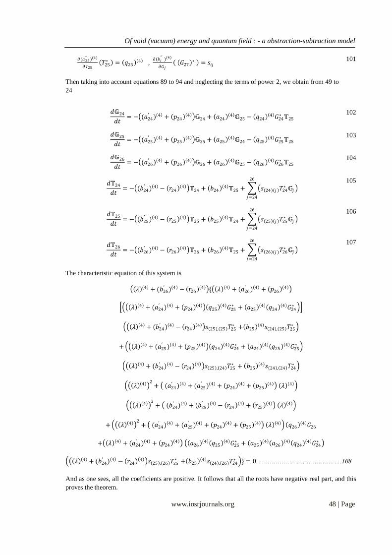
Of void (vacuum) energy and quantum field : - a abstraction-subtraction model

www.iosrjournals.org 48 | Page

𝜕(𝑎25′′ ) 4

𝜕𝑇25 𝑇25

∗ = 𝑞25 4 ,

𝜕(𝑏𝑖′′ ) 4

𝜕𝐺𝑗 𝐺27

∗ = 𝑠𝑖𝑗 101

Then taking into account equations 89 to 94 and neglecting the terms of power 2, we obtain from 49 to

24

𝑑𝔾24

𝑑𝑡= − (𝑎24

′ ) 4 + 𝑝24 4 𝔾24 + 𝑎24

4 𝔾25 − 𝑞24 4 𝐺24

∗ 𝕋25 102

𝑑𝔾25

𝑑𝑡= − (𝑎25

′ ) 4 + 𝑝25 4 𝔾25 + 𝑎25

4 𝔾24 − 𝑞25 4 𝐺25

∗ 𝕋25 103

𝑑𝔾26

𝑑𝑡= − (𝑎26

′ ) 4 + 𝑝26 4 𝔾26 + 𝑎26

4 𝔾25 − 𝑞26 4 𝐺26

∗ 𝕋25 104

𝑑𝕋24

𝑑𝑡= − (𝑏24

′ ) 4 − 𝑟24 4 𝕋24 + 𝑏24

4 𝕋25 + 𝑠 24 𝑗 𝑇24∗ 𝔾𝑗

26

𝑗 =24

105

𝑑𝕋25

𝑑𝑡= − (𝑏25

′ ) 4 − 𝑟25 4 𝕋25 + 𝑏25

4 𝕋24 + 𝑠 25 𝑗 𝑇25∗ 𝔾𝑗

26

𝑗 =24

106

𝑑𝕋26

𝑑𝑡= − (𝑏26

′ ) 4 − 𝑟26 4 𝕋26 + 𝑏26

4 𝕋25 + 𝑠 26 (𝑗 )𝑇26∗ 𝔾𝑗

26

𝑗 =24

107

The characteristic equation of this system is

𝜆 4 + (𝑏26′ ) 4 − 𝑟26

4 { 𝜆 4 + (𝑎26′ ) 4 + 𝑝26

4

𝜆 4 + (𝑎24′ ) 4 + 𝑝24

4 𝑞25 4 𝐺25

∗ + 𝑎25 4 𝑞24

4 𝐺24∗

𝜆 4 + (𝑏24′ ) 4 − 𝑟24

4 𝑠 25 , 25 𝑇25∗ + 𝑏25

4 𝑠 24 , 25 𝑇25∗

+ 𝜆 4 + (𝑎25′ ) 4 + 𝑝25

4 𝑞24 4 𝐺24

∗ + 𝑎24 4 𝑞25

4 𝐺25∗

𝜆 4 + (𝑏24′ ) 4 − 𝑟24

4 𝑠 25 , 24 𝑇25∗ + 𝑏25

4 𝑠 24 , 24 𝑇24∗

𝜆 4 2

+ (𝑎24′ ) 4 + (𝑎25

′ ) 4 + 𝑝24 4 + 𝑝25

4 𝜆 4

𝜆 4 2

+ (𝑏24′ ) 4 + (𝑏25

′ ) 4 − 𝑟24 4 + 𝑟25

4 𝜆 4

+ 𝜆 4 2

+ (𝑎24′ ) 4 + (𝑎25

′ ) 4 + 𝑝24 4 + 𝑝25

4 𝜆 4 𝑞26 4 𝐺26

+ 𝜆 4 + (𝑎24′ ) 4 + 𝑝24

4 𝑎26 4 𝑞25

4 𝐺25∗ + 𝑎25

4 𝑎26 4 𝑞24

4 𝐺24∗

𝜆 4 + (𝑏24′ ) 4 − 𝑟24

4 𝑠 25 , 26 𝑇25∗ + 𝑏25

4 𝑠 24 , 26 𝑇24∗ } = 0 …………………………………….108

And as one sees, all the coefficients are positive. It follows that all the roots have negative real part, and this

proves the theorem.

Of void (vacuum) energy and quantum field : - a abstraction-subtraction model

www.iosrjournals.org 49 | Page

AN EPILOGUE ON VACUUM ENERGY,QUANTUM FIELD,ZERO POINT

ENERGY,DARK MATTER AND THEIR INTERRELATIONSHIPS AND

RAMIFICATIONS OF RESULTS OBTAINED ON THEM: Current models of the universe assume that is close to one. For example, in the inflationary

theory a truly stupendous expansion is assumed to have occurred early in the history of the universe. About

10-34 seconds after the creation, when the temperature was perhaps one thousand trillion degrees, a bubble no

more than 10-24 cm across might have undergone an expansion by a factor of maybe 1050! At about 10-

32 seconds this expansion stopped, leaving the bubble 1026cm across (that is, 100 million light years).

However, the bit of the universe we can observe would have been, after inflation, only a few centimeters

across After 10-32 seconds, or so, the normal big bang evolution takes over. The fantastic stretching of space

during inflation renders the observable universe geometrically flat .This is because the observable universe

would be but a tiny patch of a universe that may be a trillion trillion times larger. Even if the geometry of the

universe were initially highly curved the observable part of it is such a small patch that it would nonetheless

appear to us as spatially flat, just as a small patch of the Earth's surface appears flat. Moreover, any weird

particles or spacetime distortions that may have existed when the universe came into being would have been

diluted far out of sight; we would not expect to find any such oddities in our neck of the woods. Lastly, the

microwave background radiation, which was already uniform and isotropic within the initial bubble, would

have remained so after inflation, which explains why the radiation at opposite sides of the sky has the same

temperature; these patches of sky were once in casual contact (much less than 10-24 cm apart) but were then

pushed far apart by inflation.

DARK ENERGY AND VACUUM ENERGY

Alas, Ω is observed to be much less than unity Therefore, if we nonetheless insist that Ω=1 we is forced to

conclude that the luminous matter we observe forms only a part of the total energy in the universe. The

deficit must therefore be made up by some other unknown source of energy. This could be dark matter.

Much more interesting and much more mysterious: the possible existence of vacuum energy; or perhaps an

admixture of the two.

Within the context of a general relativistic description of the universe there is two critical parameters that

determine the global properties of the universe: The Hubble constant H0 and the deceleration parameter q0. If

the universe is expanding today, it must have been expanding faster in the past provided that it is filled with

normal matter and energy. This is because the gravitational force of normal matter is always attractive and

therefore slows down the expansion. The deceleration parameter, as the name suggests, is a measure of how

much the expansion has slowed since the big bang. We have already encountered Hubble's law

Z = d H0/c,

Where Z is the redshift of a galaxy and d its (proper) distance from us. This law is valid only for small

redshifts, say less than about 0.2; that is, for galaxies that are not too distant. For very distant galaxies we

need a more accurate formula. We need this because when we look at very distant galaxies we are looking

into the distant past when the expansion rate was, presumably, greater. A more accurate formula that takes

account of the universal deceleration is

Z = d H0/c + (1+q0)(d H0/c)2/2.

In practice, cosmologists do not use the proper distance d, directly, but rather use a distance scale, called the

luminosity distance, dL, which is determined by requiring that the inverse square law

f = L/4πdL2

hold true even for an expanding universe. (In a static, flat universe both distance scales coincide.) Here f is

the measured flux (energy per square meter per second) and L is the absolute luminosity (energy per second).

Of void (vacuum) energy and quantum field : - a abstraction-subtraction model

www.iosrjournals.org 50 | Page

The luminosity distance is convenient because it can be determined from measuring f and determining L,

only.

MODEL THEORYAND LIMIT OF FINITE LINEAR ORDERINGS TO EXPLAIN THE

STRUCTURE OF VACUUM ENERGY AND QUANTUM FIELD: In model theory, the age of a structure (or model) A is the class of all finitely generated structures

which are embeddable in A (i.e. isomorphic to substructures of A). This concept is central in the construction

of a Fraïssé limit. The main point of Fraïssé's construction is to show how one can approximate a structure by

its finitely generated substructures. Thus for example the age of any dense linear order without

endpoints (DLO), is precisely the set of all finite linear orderings, which are distinguished up to

isomorphism only by their size. Thus the age of any DLO is countable. This shows in a way that a DLO is a

kind of limit of finite linear orderings.

Amalgamation property

For any structures A, B and C in K such that A is embeddable in both B and C, there exists D in K to

which B and C are both embeddable by embeddings which coincide on the image of A in both structures. In

that case, there is a unique countable structure, up to isomorphism, that has age K and is homogeneous. In this

context, Homogeneous means that any isomorphism between two finitely generated substructures can be

extended to an automorphism of the whole structure. Again, an example of this situation is the ordered set of

rational numbers . It is the unique (up to isomorphism) homogenous countable structure whose age

is the set of all finite linear orderings. Note that the ordered set of natural numbers has the same age

as a DLO, but it is not homogenous since if we map {1, 3} to {5, 6}, it would not extend to any

automorphism f since there should be an element between and . The same applies

to integers.

ANTHROPIC PRINCIPLE-EVERYTHING HAS AGE - VACUUM ENERGY AND

QUANTUM FIELD IN COSMOS HAS AGE

In astrophysics and cosmology, the anthropic principle is the consideration that observations of the

physical Universe must be compatible with the conscious life that observes it. Some proponents of the

anthropic principle reason that it explains why the Universe has the age and the fundamental physical

constants necessary to accommodate conscious life. As a result, they believe that the fact is unremarkable that

the universe's fundamental constants happen to fall within the narrow range thought to be compatible with

life. The strong anthropic principle (SAP) as explained by Barrow and Tipler (see variants) states that this is

all the case because the Universe is compelled, in some sense, for conscious life to eventually

emerge. Douglas Adams used the metaphor of a living puddle examining its own shape, since, to those living

creatures, the universe may appear to fit them perfectly (while in fact, they simply fit the universe perfectly).

Critics of the SAP argue in favor of a weak anthropic principle (WAP) similar to the one defined by Brandon

Carter, which states that the universe‘s ostensible fine tuning is the result of selection bias: i.e., only in a

universe capable of eventually supporting life will there be living beings capable of observing any such fine

tuning, while a universe less compatible with life will go unbeheld.

The principle was formulated as a response to a series of observations that the laws of nature and

parameters of the Universe take on values that are consistent with conditions for life as we know it rather

than a set of values that would not be consistent with life on Earth. The anthropic principle states that this

is a necessity, because if life were impossible, no one would know it. That is, it must be possible to

observe some Universe, and hence, the laws and constants of any such universe must accommodate that

possibility. The term anthropic in "anthropic principle" has been argued to be a misnomer, an anachronism

both in predicational anteriority and character constitution.. Anthropic principle is a tautology or truism. In

1961, Robert Dicke noted that the age of the universe, as seen by living observers, cannot be random. Instead,

Of void (vacuum) energy and quantum field : - a abstraction-subtraction model

www.iosrjournals.org 51 | Page

biological factors constrain the universe to be more or less in a "golden age," neither too young nor too

old. If the universe were one tenth as old as its present age, there would not have been sufficient time to build

up appreciable levels of metallicity (levels of elements besides hydrogen and helium) especially carbon,

by nucleosynthesis. Small rocky planets did not yet exist. If the universe were 10 times older than it actually

is, most stars would be too old to remain on the main sequence and would have turned into white dwarfs,

aside from the dimmest red dwarfs, and stable planetary systems would have already come to an end. Thus

Dicke explained away the rough coincidence between large dimensionless numbers constructed from the

constants of physics and the age of the universe, a coincidence which had inspired Dirac's varying-G theory.

Dicke later reasoned that the density of matter in the universe must be almost exactly the same as

the critical density needed to prevent the Big Crunch (the "Dicke coincidences" argument). The most recent

measurements may suggest that the observed density of baryonic matter, and some theoretical predictions of

the amount of dark matter account for about 30% of this critical density, with the rest contributed by

a cosmological constant. Steven Weinberg gave an anthropic explanation for this fact: he noted that the

cosmological constant has a remarkably low value, some 120 orders of magnitude smaller than the

value particle physics predicts. If the cosmological constant were more than about 10 times its observed

value, then, it shall produce universe that would suffer catastrophic inflation, which would preclude the

formation of stars, and hence life.

The observed values of the dimensionless physical constants (such as the fine-structure constant)

governing the four fundamental interactions are balanced as if fine-tuned to permit the formation of

commonly found matter and subsequently the emergence of life. A slight increase in the strong nuclear

force would bind the dineutron and the diproton, and nuclear fusion would have converted all hydrogen in

the early universe to helium. Water and the long-lived stable stars essential for the emergence of life as we

know it would not exist. More generally, small changes in the relative strengths of the four fundamental

interactions can greatly affect the universe's age, structure, and capacity for life. Carter defined two forms of

the Anthropic Principle, a "weak" one which referred only to anthropic selection of

privileged spacetime locations in the universe, and a more controversial "strong" form which addressed the

values of the fundamental constants of physics.Roger Penrose explained the weak form as follows:

"The argument of weak anthropic principle can be used to explain why the conditions happen to be

just right for the existence of (intelligent) life on the earth at the present time. For if they were not just right,

then we should not have found ourselves to be here now, but somewhere else, at some other appropriate time.

This principle was used very effectively by Brandon Carter and Robert Dicke to resolve an issue that had

puzzled physicists for a good many years. The issue concerned various striking numerical relations that are

observed to hold between the physical constants (the gravitational constant, the mass of the proton, the age of

the universe, etc.). A puzzling aspect of this was that some of the relations hold only at the present epoch in

the earth's history, so we appear, coincidentally, to be living at a very special time (give or take a few million

years). This was later explained, by Carter and Dicke, by the fact that this epoch coincided with the lifetime

of what are called main-sequence stars, such as the sun. At any other epoch, so the argument ran, there would

be no intelligent life around in order to measure the physical constants in question — so the coincidence had

to hold, simply because there would be intelligent life around only at the particular time that the coincidence

did hold!"(—The Emperor's New Mind, Chapter 10)

First, we can use our own existence to make "predictions" about the parameters. But second, "as a

last resort", we can convert these predictions into explanations by assuming that there is more than one

Universe, in fact a large and possibly infinite collection of universes, something that is now called

a multiverse ("world ensemble" was Carter's term), in which the parameters (and perhaps the laws of physics)

vary across universes. The strong principle then becomes an example of a selection effect, exactly analogous

to the weak principle. Postulating a multiverse is certainly a radical step, but taking it could provide at least a

partial answer to a question which had seemed to be out of the reach of normal science: "why do

the fundamental laws of physics take the particular form we observe and not another?"(See authors

Of void (vacuum) energy and quantum field : - a abstraction-subtraction model

www.iosrjournals.org 52 | Page

‗Measurement disturbs Quantum Mechanical Explanation), This apparantely mean that perception

changes reality. Perception is not reality.

Carter was not the first to invoke some form of the anthropic principle. In fact, the evolutionary

biologist Alfred Russel Wallace anticipated the anthropic principle as long ago as 1904: "Such a vast and

complex universe as that which we know exists around us, may have been absolutely required ... in order to

produce a world that should be precisely adapted in every detail for the orderly development of life

culminating in man." In 1957, Robert Dicke wrote: "The age of the Universe 'now' is not random but

conditioned by biological factors ... changes in the values of the fundamental constants of physics] would

preclude the existence of man to consider the problem. And how is it every things that happens could be

understood in mathematical terms? Somebody knew that we are coming and also possess knowledge of

Mathematics!

STRONG AND WEAK ANTHROPIC PRINCIPLE: Strong anthropic principle (SAP) (Barrow and Tipler): "The Universe must have those

properties which allow life to develop within it at some stage in its history. This looks very similar to

Carter's SAP, but unlike the case with Carter's SAP, the "must" is an imperative, as shown by the

following three possible elaborations of the SAP, each proposed by Barrow and Tipler"There exists one

possible Universe 'designed' with the goal of generating and sustaining 'observers.'

This can be seen as simply the classic design argument(intelligent grand design) restated in the garb of

contemporary cosmology. It implies that the purpose of the universe is to give rise to intelligent life,

with the laws of nature and their fundamental physical constants set to ensure that life as we know it

will emerge and evolve."Observers are necessary to bring the Universe into being."Presence of

observers is necessary the existence of space time continuum. Perception of observers is essential

functional prerequisite for the existence of the Universe."An ensemble of other different universes is

necessary for the existence of our Universe. "

Although philosophers have discussed related concepts for centuries, in the early 1970s the only

genuine physical theory yielding a multiverse of sorts was the many worlds interpretation of quantum

mechanics. This would allow variation in initial conditions, but not in the truly fundamental constants.

Since that time a number of mechanisms for producing a multiverse have been suggested: (see the

review by Max Tegmark). An important development in the 1980s was the combination of inflation

theory with the hypothesis that some parameters are determined by symmetry breaking in the early

universe, which allows parameters previously thought of as "fundamental constants" to vary over very

large distances, thus eroding the distinction between Carter's weak and strong principles. At the

beginning of the 21st century, the string landscape emerged as a mechanism for varying essentially all

the constants, including the number of spatial dimensions.The anthropic idea that fundamental

parameters are selected from a multitude of different possibilities (each actual in some universe or

other) contrasts with the traditional hope of physicists for a theory of everything having no free

parameters: as Einstein said, "What really interests me is whether God had any choice in the creation

of the world." Quite recently, proponents of the leading candidate for a "theory of everything", string

theory, proclaimed "the end of the anthropic principle since there would be no free parameters to

select. Ironically, string theory now seems to offer no hope of predicting fundamental parameters, and

now some who advocate it invoke the anthropic principle as well.

The modern form of a design argument is put forth by Intelligent design. Proponents of

intelligent design often cite the fine-tuning observations that (in part) preceded the formulation of the

anthropic principle by Carter as a proof of an intelligent designer. Opponents of intelligent design are

not limited to those who hypothesize that other universes exist; they may also argue, anti-anthropically,

that the universe is less fine-tuned than often claimed, or that accepting fine tuning as a brute fact is less

Of void (vacuum) energy and quantum field : - a abstraction-subtraction model

www.iosrjournals.org 53 | Page

astonishing than the idea of an intelligent creator. Furthermore, even accepting fine

tuning, Sober (2005) and Ikeda and Jefferys, argue that the Anthropic Principle as conventionally

stated actually undermines intelligent design; see fine-tuned universe.

Don Page criticized the entire theory of cosmic inflation. He emphasized those initial conditions which made

possible a thermodynamic arrow of time in a universe with a Big Bang origin, must include the assumption

that at the initial singularity, the entropy of the universe was low and therefore extremely improbable. Paul

Davies rebutted this criticism by invoking an inflationary version of the anthropic principle. While Davies

accepted the premise that the initial state of the visible Universe (which filled a microscopic amount of space

before inflating) had to possess a very low entropy value — due to random quantum fluctuations — to

account for the observed thermodynamic arrow of time, he deemed this fact an advantage for the theory. That

the tiny patch of space from which our observable Universe grew had to be extremely orderly, to allow the

post-inflation universe to have an arrow of time, makes it unnecessary to adopt any "ad hoc" hypotheses

about the initial entropy state, hypotheses other Big Bang theories require.

String theory and vacuum energy

String theory predicts a large number of possible universes, called the "backgrounds" or "vacua."

The set of these vacua is often called the "multiverse" or "anthropic landscape" or "string landscape." Leonard Susskind has argued that the existence of a large number of vacua puts anthropic reasoning on firm ground:

only universes whose properties are such as to allow observers to exist are observed, while a possibly much

larger set of universes lacking such properties go unnoticed.

Steven Weinberg believes the Anthropic Principle may be appropriated by cosmologists committed

to nontheism, and refers to that Principle as a "turning point" in modern science because applying it to the

string landscape "...may explain how the constants of nature that we observe can take values suitable for life

without being fine-tuned by a benevolent creator." Others, most notably David Gross but also Lubos

Motl, Peter Woit, and Lee Smolin, argue that this is not predictive. Max Tegmark, Mario Livio, and Martin

Rees[ argue that only some aspects of a physical theory need be observable and/or testable for the theory to

be accepted, and that many well-accepted theories are far from completely testable at present.

When water freezes into ice, the ice floats because ice is less dense than liquid water. This is one

possible example of the anthropic principle, because if ice did not float, it might have been difficult or

impossible for living organisms to have existed in water; without the insulating properties of a top ice layer,

lakes and ponds would tend to freeze solid and thaw very little during warmer periods. This principle has

been criticized as neglecting the existence of the tropical zone and other warmer climates.

Ice is unusual in that it is approximately 9% less dense than liquid water. Water is the only known non-

metallic substance to expand when it freezes. The density of ice is 0.9167 g/cm3at 0°C, whereas water has a

density of 0.9998 g/cm3 at the same temperature. Liquid water is densest, essentially 1.00 g/cm3, at 4°C and

becomes less dense as the water molecules begin to form the hexagonal crystals of ice as the freezing point is

reached. This is due to hydrogen bonding dominating the intermolecular forces, which results in a packing of

molecules less compact in the solid.

The Anthropic Cosmological Principle,Dark Energy and Vacuum Energy:

Barrow and Tipler carefully distinguish teleological reasoning from eutaxiological reasoning; the

former asserts that order must have a consequent purpose; the latter asserts more modestly that order

must have a planned cause. They attribute this important but nearly always overlooked distinction to

an obscure 1883 book by L. E. HicksSeeing little sense in a principle requiring intelligent life to emerge

while remaining indifferent to the possibility of its eventual extinction, Barrow and Tipler propose

the:"Final anthropic principle (FAP): Intelligent information-processing must come into existence in the

Universe, and, once it comes into existence, it will never die out."

FAP places strong constraints on the structure of the universe, constraints developed further in

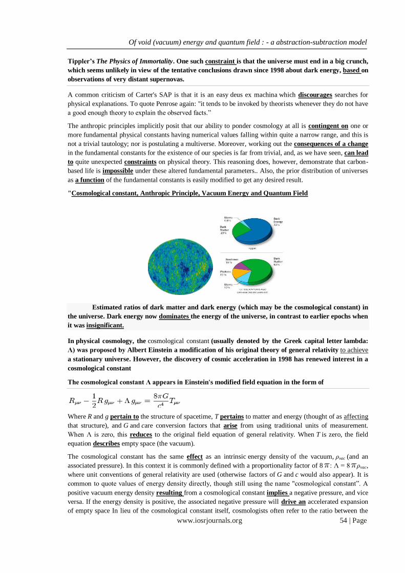
Of void (vacuum) energy and quantum field : - a abstraction-subtraction model

www.iosrjournals.org 54 | Page

Tippler‘s The Physics of Immortality. One such constraint is that the universe must end in a big crunch,

which seems unlikely in view of the tentative conclusions drawn since 1998 about dark energy, based on

observations of very distant supernovas.

A common criticism of Carter's SAP is that it is an easy deus ex machina which discourages searches for

physical explanations. To quote Penrose again: "it tends to be invoked by theorists whenever they do not have

a good enough theory to explain the observed facts.‖

The anthropic principles implicitly posit that our ability to ponder cosmology at all is contingent on one or

more fundamental physical constants having numerical values falling within quite a narrow range, and this is

not a trivial tautology; nor is postulating a multiverse. Moreover, working out the consequences of a change

in the fundamental constants for the existence of our species is far from trivial, and, as we have seen, can lead

to quite unexpected constraints on physical theory. This reasoning does, however, demonstrate that carbon-

based life is impossible under these altered fundamental parameters.. Also, the prior distribution of universes

as a function of the fundamental constants is easily modified to get any desired result.

"Cosmological constant, Anthropic Principle, Vacuum Energy and Quantum Field

Estimated ratios of dark matter and dark energy (which may be the cosmological constant) in

the universe. Dark energy now dominates the energy of the universe, in contrast to earlier epochs when

it was insignificant.

In physical cosmology, the cosmological constant (usually denoted by the Greek capital letter lambda:

Λ) was proposed by Albert Einstein a modification of his original theory of general relativity to achieve

a stationary universe. However, the discovery of cosmic acceleration in 1998 has renewed interest in a

cosmological constant

The cosmological constant Λ appears in Einstein's modified field equation in the form of

Where R and g pertain to the structure of spacetime, T pertains to matter and energy (thought of as affecting

that structure), and G and care conversion factors that arise from using traditional units of measurement.

When Λ is zero, this reduces to the original field equation of general relativity. When T is zero, the field

equation describes empty space (the vacuum).

The cosmological constant has the same effect as an intrinsic energy density of the vacuum, ρvac (and an

associated pressure). In this context it is commonly defined with a proportionality factor of 8 : Λ = 8 ρvac,

where unit conventions of general relativity are used (otherwise factors of G and c would also appear). It is

common to quote values of energy density directly, though still using the name "cosmological constant‖. A

positive vacuum energy density resulting from a cosmological constant implies a negative pressure, and vice

versa. If the energy density is positive, the associated negative pressure will drive an accelerated expansion

of empty space In lieu of the cosmological constant itself, cosmologists often refer to the ratio between the

Of void (vacuum) energy and quantum field : - a abstraction-subtraction model

www.iosrjournals.org 55 | Page

energy density due to the cosmological constant and the critical density of the universe. This ratio is usually

denoted . In a flat universe corresponds to the fraction of the energy density of the Universe due to

the cosmological constant. Note that this definition is tied to the critical density of the present cosmological

era: the critical density changes with cosmological time, but the energy density due to the cosmological

constant remains unchanged throughout the history of the universe. Another ratio that is used by scientists is

the equation of state which is the ratio of pressure that dark energy puts on the Universe to the energy per

unit volume.

VACUUM ENERGY CAUSE OF EXPANSION OF THE UNIVERSE: In fact adding the cosmological constant to Einstein's equations does not lead to a static universe at

equilibrium because the equilibrium is unstable: if the universe expands slightly, then the expansion

releases vacuum energy, which causes yet more expansion. Likewise, a universe which contracts slightly will

continue contracting. Empirically, the onslaught of cosmological data in the past decades strongly suggests

that our universe has a positive cosmological constant. Finally, it should be noted that some early

generalizations of Einstein's gravitational theory, known as classical unified field theories, either introduced a

cosmological constant on theoretical grounds or found that it arose naturally from the mathematics. For

example, Sir Arthur Stanley Eddington claimed that the cosmological constant version of the vacuum field

equation expressed the "epistemological" property that the universe is "self-gauging", and Erwin

Schrödinger's pure-affine theory using a simple vibrational principle produced the field equation with a

cosmological t distance–redshift relation for Type Ia supernovae indicated that the expansion of the universe

is accelerating. When combined with measurements of the cosmic microwave background radiation these

implied a value of ,[7] a result which has been supported and refined by more recent

measurements. There are other possible causes of an accelerating universe, such as quintessence, but the

cosmological constant is in most respects the simplest solution. Thus, the current standard model of

cosmology, the Lambda-CDM model, includes the cosmological constant, which is measured to be on the

order of 10−52 m−2, in metric units. Multiplied by other constants that appear in the equations, it is often

expressed as 10−35 s−2, 10−47 GeV4, 10−29 g/cm3. In terms of Planck units, and as a natural dimensionless value,

the cosmological constant, λ, is on the order of 10−122.

As was only recently seen, by works of 't Hooft, Susskind and others, a positive cosmological

constant has surprising consequences, such as a finite maximum entropy of the observable universe (see

the holographic principle).

A problem arises with inclusion of the cosmological constant in the standard model: i.e., the

appearance of solutions with regions of discontinuities (see classification of discontinuities at typical matter

density ) Another investigation found the cosmological time, dt, diverges for any finite interval, ds,

associated with an observer approaching the cosmological horizon, representing a physical limit to

observation for the standard model when the cosmological term is included. This is a key requirement for a

complete interpretation / definition of astronomical observations, particularly pertaining to the nature of

dark energy and the cosmological constant. All of these findings should be considered major shortcomings

of the standard model, but only when the cosmological constant term is included.

ZERO POINT ENERGY OF THE VACUUM AND (E/EB)COSMOLOGICAL CONSTANT

–AN UNSOLVED PROBLEM IN PHYSICS

A major outstanding problem is that most quantum field theories predict a huge value for the

quantum vacuum. A common assumption is that the quantum vacuum is equivalent to the cosmological

constant. Although no theory exists that supports this assumption, arguments can be made in its favor. Such

arguments are usually based on dimensional analysis and effective field theory. If the universe is described

by an effective local quantum field theory down to the Planck scale, then we would expect a cosmological

constant of the order of . As noted above, the measured cosmological constant is smaller than this by a

factor of 10−120. This discrepancy has been called "the worst theoretical prediction in the history of

Of void (vacuum) energy and quantum field : - a abstraction-subtraction model

www.iosrjournals.org 56 | Page

physics!".Some supersymmetric theories require /need a cosmological constant that is exactly zero, which

further complicates things. Weinberg explains that if the vacuum energy took different values in different

domains of the universe, then observers would necessarily measure values similar to that which is observed:

the formation of life-supporting structures would be suppressed in domains where the vacuum energy is

much larger. Specifically, if the vacuum energy is negative and its absolute value is substantially larger than it

appears to be in the observed universe (say, a factor of 10 larger), holding all other variables (e.g. matter

density) constant, that would mean that the universe is closed; furthermore, its lifetime would be shorter than

the age of our universe, possibly too short for the intelligent life to form. On the other hand, a universe with a

large positive cosmological constant would expand too fast, preventing galaxy formation. According to

Weinberg, domains where the vacuum energy are compatible with life would be comparatively rare. Using

this argument, Weinberg predicted that the cosmological constant would have a value of less than a hundred

times the currently accepted value In 1992 Weinberg refined this prediction of the cosmological constant to 5

to 10 times the matter density.

This argument depends on a lack of a variation of the distribution (spatial or otherwise) in the

vacuum energy density, as would be expected if the dark energy were the cosmological constant. There is

no evidence that the vacuum energy does vary, but it may be the case if, for example, the vacuum energy is

(even in part) the potential of a scalar field such as the residual inflaton (also see quintessence). Another

theoretical approach that deals with the issue is that of multiverse theories - predicting a large number of

"parallel" universes, possibly with different laws of physics and/or values of fundamental constants. Again,

the anthropic principle states that we can only live in one of the universes that is compatible with some form

of intelligent life. Critics claim that these theories, when used as an explanation for fine-tuning, commit

the inverse gambler's fallacy.

More recent work has suggested the problem may be indirect evidence of a cyclic universe possibly

as allowed by string theory. With every cycle of the universe (Big Bang then eventually a Big Crunch) taking

about a trillion (1012) years, "the amount of matter and radiation in the universe is reset, but the cosmological

constant is not. Instead, the cosmological constant gradually diminishes over many cycles to the small value

observed today." Fecund universes theory, which assumes universes have "offspring" through the creation

of black holes, and that these offspring universes have values of physical constants that depend on these of

the mother universe. But Lee Smolin assumes that conditions for carbon based life are similar to conditions

for black hole creation, which would change the a priori distribution of universes such that universes

containing life would be likely. Weak version is mere tautological and the stronger version is epistemological

with ontological predication without phenomenological methodologies.

In the context of cosmology the cosmological constant is a homogeneous energy density that

causes the expansion of the universe to accelerate. Originally proposed early in the development of general

relativity in order to allow a static universe solution it was subsequently abandoned when the universe was

found to be expanding. Now the cosmological constant is invoked to explain the observed acceleration of the

expansion of the universe. The cosmological constant is the simplest realization of dark energy, which the

more generic name is given to the unknown cause of the acceleration of the universe. Its existence is also

predicted by quantum physics, where it enters as a form of vacuum energy, although the magnitude predicted

by quantum theory does not match that observed in cosmology.

At the time, observations of our universe were limited primarily to stars in our own galaxy, so there

was indeed observational evidence justifying the assumption that the universe was static. Einstein's goal was

to obtain a Universe that satisfied Mach's principle of the relativity of inertia (for a historical discussion

see Pais 1982, Sect 15e), and construct a cosmology that was finite, yet stable against gravitational collapse.

The attempt proved futile, as shortly thereafter de Sitter (1917) demonstrated an empty universe solution to

Einstein's equations (allowing inertia relative to space empty of matter) and Friedman (1922) derived

solutions to Einstein's equations that corresponded to an expanding universe. These results could be

considered a prediction that the universe must be expanding or contracting, a remarkable implication of

general relativity that was later borne out by observation. When Hubble observationally discovered the

Of void (vacuum) energy and quantum field : - a abstraction-subtraction model

www.iosrjournals.org 57 | Page

expansion of the universe Einstein finally abandoned the cosmological constant completely (Einstein 1931).

As of the early 1990s there were tantalizing hints that the cosmological constant might again be

needed. The universe appeared to be younger than the oldest stars it contained (age of the stars (e) age of the

universe), a feature that was remedied if the universe was currently in an accelerating phase. Number counts

of galaxies indicated that the volume contained within a solid angle at high redshift was larger than expected

in a decelerating universe. Theoretical arguments from inflation and later observational results from

the cosmic microwave background radiation indicated that the universe should be flat, but observations of

large scale structure indicated that the matter density was inadequate to achieve this -- vacuum energy could

make up the shortfall.

The mass-energy composition of the Universe. The cosmological constant is one possible form(=)

of dark energy, which is believed to be behind or produces the acceleration of the expansion Universe. The

High-Z supernova team and the Supernova Cosmology project both discovered that high-redshift supernovae

were fainter than expected for a decelerating universe and that the difference could be

explained/balanced(e) if there was a cosmological constant of just the right magnitude needed to make the

universe flat. This was a dramatic convergence of observation and theory. Since then increasingly accurate

probes have confirmed to high precision the need for dark energy,(for the production of the flat universe) but

the nature of the dark energy is now the issue being investigated. As of 2010 the measured properties of dark

energy remain consistent with those of a cosmological constant(implies dark energy=cosmological constant).

However, massive observing efforts are underway to test whether this is the correct explanation for the

acceleration or whether some other sort of dark energy, perhaps one that changes (e and eb)with time or one

that is motivated(eb) by some form of quantum gravity, is needed to (eb)explain the acceleration we see.

The physics of the cosmological constant and Vacuum Energy: To explore more deeply the nature of the Universe, we must use the mathematical language in

Einstein's general relativity to relate the geometry of space-time (expressed by the metric tensor, gμν) to the

energy content of the universe, (expressed by the energy-momentum tensor, Tμν).Arguably, one of

Einstein's most significant discoveries was that the distribution of energy determines the geometry of space-

time, which is encoded (incorporated)in his field equation,

Rμν−12Rgμν=8πGTμν ,-----(1)

where G is the gravitational constant. Although this is the simplest form of the equations the freedom remains

to add a constant term. This "cosmological constant" was what Einstein added in order to achieve a static

universe, and it is given the symbol Λ .

Rμν−12Rgμν+Λgμν=8πGTμν---(2) When Λ is positive it acts as a repulsive force.

Vacuum Energy

Of void (vacuum) energy and quantum field : - a abstraction-subtraction model

www.iosrjournals.org 58 | Page

The equation of state, w, determines (eb) the relationship between pressure and density in a material

according to w=p/ρ . Here are some examples of the equation of state for common fluids. When matter is at

rest (pressure less dust) it has w=0 , but as it picks up velocity (v) its equation of state increases

until w→1/3 as v→c .

VACUUM ENERGY AND UNCERTAINTY PRINCIPLE: Vacuum energy arises naturally in quantum mechanics due to the uncertainty principle. In

particle physics the vacuum refers (=) to the ground state of the theory -- the lowest energy

configuration. The uncertainty principle does not allow e(eb) states of exactly zero energy, even in

vacuum (virtual particles are created). Since in general relativity all forms of energy gravitate, this

ground state vacuum energy impacts the dynamics of the expansion of the universe.

The early cosmic inflation, when taken along with the recent observations that the universe is currently

dominated by a low density vacuum energy, leads to at least two potential problems which modern

cosmology must address. First, there is the old cosmological constant problem, with a new twist: the

coincidence problem. Secondly, cosmology still lacks a model to predict the observed current cosmic

acceleration and to determine whether or not there is a future exit out of this state (as previously in the

inflationary case). This constitutes (what is called here) a dynamical problem. In this article a framework is

proposed to address these two problems, based on treating the cosmic background vacuum (dark) energy as

both dynamical and interacting. The universe behaves as a vacuum-driven cosmic engine which, in search of

equilibrium, always back-reacts to vacuum-induced accelerations by increasing its inertia (internal energy)

through vacuum energy dissipation. The process couples cosmic vacuum (dark) energy to matter to produce

future-directed increasingly comparable amplitudes in these fields by setting up oscillations in the decaying

vacuum energy density and corresponding sympathetic ones in the matter fields. By putting bounds on the

relative magnitudes of these coupled oscillations the model offers a natural and conceptually simple channel

to discuss the coincidence problem, while also suggesting a way to deal with the dynamical problem. A result

with useful observational implications is an equation of state w(t) which specifically predicts a variable,

quasi-periodic, acceleration for the current universe. This result can be directly tested by future observational

techniques such as SNAP.(( Manasse R. Mbonye)

Vacuum energy should not have any dissipative processes such as heat conduction or viscosity, so it should

take the form of a perfect fluid,

Tμν=(ρ+p)UμUν+pgμν.(3)

In order to maintain Lorentz invariance, vacuum energy should also have no preferred direction. Therefore

the first term in the perfect fluid energy tensor must be zero, requiring

pvac=−ρvac,(4)

which corresponds to an equation of state wvac=pvac/ρvac=−1 , and results in an energy-momentum tensor

for vacuum energy,

Tvacμν=pvacgμν=−ρvacgμν.(5)

Equivalence of Cosmological Constant and Vacuum Energy

Of void (vacuum) energy and quantum field : - a abstraction-subtraction model

www.iosrjournals.org 59 | Page

We can split the energy-momentum tensor into a term describing the matter and energy, and a term describing

the vacuum, Tμν=Tmatterμν+Tvacμν . Einstein's equation including vacuum energy becomes,

Rμν−12Rgμν=8πG(Tmatterμν−ρvacgμν).(6)

Recall that the cosmological constant enters Einstein's equation in the form,

Rμν−12Rgμν+Λgμν=8πGTμν.

So vacuum energy and the cosmological constant have identical behaviour in general relativity, as long as the

vacuum energy density is identified with,

ρvac=Λ8πG.(7)

In an homogeneous, isotropic universe the geometry is defined by the Friedman-Lemaître-Robertson-Walker

metric (FLRW metric) and the dynamics of the universe are governed by the Friedman equations (Friedmann

equations). The dynamics are driven by the energy content of the universe and the equation of state of the

components that make up the energy density. The equation of state relates density ρ to pressure p according

to w=p/ρ . The cosmological constant enters these equations in the following way, where a is the scale factor

of the universe normalized to 1 at the present day, H=a˙/a is Hubble's constant (an overdot represents

differentiation with respect to time), and k is the curvature of the universe given by +1, 0, and -1 for positive,

flat, and negative curvature respectively,

H2=8πG3ρ−ka2+Λ3,(8)

a¨a=−4πG3(ρ+3p)+Λ3.(9)

These equations are more concisely written by considering both the cosmological constant and curvature as

forms of energy density (ρΛ=Λ/8πG and ρk=−3k/8πGa2). Then Eqs. (8) and (9) become

H2=8πG3∑iρi,(10)

a¨a=−4πG3∑i(ρi+3pi).(11)

The different components have different equations of state, wi , which determines how their density changes

with the expansion of the universe :

ρi=ρi0a−3(1+wi) (12)

Pressure less matter has w=0 , radiation has w=1/3 , curvature has an effective w=−1/3 , cosmological

constant has w=−1 . (We have used wΛ=−1, which implies ρΛ+3pΛ=−2ρΛ in deriving Eq. (11).)

The current energy density of each component, ρi0 , is often represented as a fraction of the critical

density, ρc=3H20/8πG , which is the energy density required to close the universe (also calculated at the

present day). Denoting this Ωi=ρi0/ρc and using Eq. (12) allows us to write

H2=H20∑iρiρc=H20∑iΩia−3(1+wi)(13)

For pressure to do work there needs to be a pressure gradient -- a relatively high pressure region next to a

relatively low pressure region -- that will then cause movement from high pressure to low. In a homogeneous

universe there are no pressure gradients, so a positive pressure does no work and has no expanding effect

(there are no low-pressure regions for it to push matter into). On the contrary, in general relativity all forms of

energy gravitate so pressure effectively pulls, strengthening the attractive force of gravity (thus the factor

of p in Eq. (9), which does not appear in Newtonian gravity). The cosmological constant has negative

pressure, w=−1 , so its general relativistic contribution counteracts the normal force of gravity and provides

an outwards acceleration. Observational evidence for the accelerating universe is now very strong, with many

different experiments covering vastly different timescales, length scales, and physical processes, all

supporting the standard ΛCDM cosmological model, in which the universe is flat with an energy density

Of void (vacuum) energy and quantum field : - a abstraction-subtraction model

www.iosrjournals.org 60 | Page

made up of about 4% baryonic matter, 23% dark matter, and 73% cosmological constant. For more detail and

references see the review by Frieman, Turner and Huterer 2008.

The critical observational result that brought the cosmological constant into its modern prominence was the

discovery that distant type Ia supernovae (0<z<1), used as standard candles, were fainter than expected in a

decelerating universe (Riess et al. 1998, Perlmutter et al. 1999). Since then many groups have confirmed this

result with more supernovae and over a larger range of redshifts. Of particular importance are the

observations that extremely high redshift (z>1) supernovae are brighter than expected, which is the

observational signature that is expected from a period of deceleration preceding our current period of

acceleration.

Conclusions: Under this category, we summarize the work done, namely the study of formulation of the

Governing Equations, necessary sine qua non attributions like accentuation and dissipation which are

essential functional prerequisite for the consummation and success of the model. It is to be stated that

primary focus and locus is of homologues nature and differentially instrumentally activities of the model

performance such as stability analysis, asymptotic analysis, solution behavior , and the sententious and

pithy prognostications under which the systems become functional or for that matter dysfunctional. We do not

write a separate conclusive note. Herein itself is mentioned the holistic and generalizational view of the work

done, as has been done in the foregoing. Imperative compatibilities and structural variabilities of the Vacuum

Energy and Quantum Field are stated in unequivocal terms. Common patterns of phenomenological

methodology, essential predications, suspensional neutralities, rational representations, conferential

extrinsicness, interfacial interference and syncopated justice the model does for the generalized goal to be

consummated is dealt with. Solutional behavior, stability analyses, asymptotic analysis bear ample

testimony, infallible observatory, and impeccable demonstration to the predicational anteriority, character

constitution, ontological consonance, primordial exactitude to the acolytish representation and apocryphal

aneurism and associated asseveration of the Governing Equations and the obtention of Stability analysis

which is dealt in detail ,stating what happens to the singularities, anti generalities or event at

contracted points, and normal performance of the model in normal conditions. This helps in the optimum

development of the system of governing equations and dynamical improvement of the conditionalities for the

instrumental efficaciousness of the stability, or reduction of asymptotic stability as the practical applications

demand. No conjecture however is made because of ignorance of such possibilities and possibilities.

Concatenated governing equations thus provide a qualitative gradient of internal structural differentiation, and

diffuse solidarity abstraction. No separate conclusion statement is made in consideration to the fact that

motivational orientation and institutionalization of pattern variables that are used have already been stated

here. At Planck’s scale there might be energetic franticness or ensorcelled frenzy of the Vacuum Energy and

Quantum Field, and these extrapolations have to be explored in detail by more eminent, erudite, and esteemed

researchers. Vacuum energy is one type of energy, which could be highly belligerently tempestuous and

temerariously reckless when put to different uses. While a tendentious testament is not provided, a first step

of a progenitor is taken for the intimate comprehension of the system. Further papers build on this

framework towards the consummation of higher theories envisioned. This on the other hand provides a

rich receptacle, reliquary repository to other researchers to study practical applications right from the simple

appliances like piston to highly sophisticated ones like in CERN

Acknowledgments The introduction is a collection of information from, articles, abstracts of the articles, paper reports,

home pages of the authors, textbooks, research papers, and various other sources including the internet

including Wikipedia. We acknowledge all authors who have contributed to the same. Should there be any act

of omission or commission on the part of the authors in not referring to the author, it is authors‘ ‗sincere

entreat, earnest beseech ,and fervent appeal to pardon such lapses as has been done or purported to have been

done in the foregoing. With great deal of compunction and contrition, the authors beg the pardon of the

respective sources. References list is only illustrative and not exhaustive. We have put all concerted efforts

Of void (vacuum) energy and quantum field : - a abstraction-subtraction model

www.iosrjournals.org 61 | Page

and sustained endeavors to incorporate the names of all the sources from which information has been

extracted. It is because of such eminent, erudite, and esteemed people allowing us to piggy ride on their

backs, we have attempted to see little forward, or so we think.

REFERENCES

[1] Dr K N Prasanna Kumar, Prof B S Kiranagi, Prof C S Bagewadi - MEASUREMENT DISTURBS EXPLANATION OF

QUANTUM MECHANICAL STATES-A HIDDEN VARIABLE THEORY - published at: "International Journal of Scientific

and Research Publications, Volume 2, Issue 5, May 2012 Edition".

[2] DR K N PRASANNA KUMAR, PROF B S KIRANAGI and PROF C S BAGEWADI -CLASSIC 2 FLAVOUR COLOR

SUPERCONDUCTIVITY AND ORDINARY NUCLEAR MATTER-A NEW PARADIGM STATEMENT - published at:

"International Journal of Scientific and Research Publications, Volume 2, Issue 5, May 2012 Edition".

[3] A HAIMOVICI: ―On the growth of a two species ecological system divided on age groups‖. Tensor, Vol 37

(1982),Commemoration volume dedicated to Professor Akitsugu Kawaguchi on his 80th birthday

[4] FRTJOF CAPRA: ―The web of life‖ Flamingo, Harper Collins See "Dissipative structures‖ pages 172-188

[5] HEYLIGHEN F. (2001): "The Science of Self-organization and Adaptivity", in L. D. Kiel, (ed) . Knowledge Management,

Organizational Intelligence and Learning, and Complexity, in: The Encyclopedia of Life Support Systems ((EOLSS), (Eolss

Publishers, Oxford) [http://www.eolss.net

[6] MATSUI, T, H. Masunaga, S. M. Kreidenweis, R. A. Pielke Sr., W.-K. Tao, M. Chin, and Y. J Kaufman (2006), ―Satellite-

based assessment of marine low cloud variability associated with aerosol, atmospheric stability, and the diurnal cycle‖, J.

Geophys. Res., 141, D17201, doi:10.1029/2005JD006097

[7] STEVENS, B, G. Feingold, W.R. Cotton and R.L. Walko, ―Elements of the microphysical structure of numerically simulated

nonprecipitating stratocumulus‖ J. Atmos. Sci., 53, 980-1006

[8] FEINGOLD, G, Koren, I; Wang, HL; Xue, HW; Brewer, WA (2010), ―Precipitation-generated oscillations in open cellular cloud

fields‖ Nature, 166 (7308) 819-852, doi: 10.1038/nature09314, Published 12-Aug 2010

[9] R WOOD ―The rate of loss of cloud droplets by coalescence in warm clouds‖ J.Geophys. Res., 141, doi:

10.1029/2006JD007553, 2006

[10] H. RUND, ―The Differential Geometry of Finsler Spaces‖, Grund. Math. Wiss. Springer-Verlag, Berlin, 195 A. Dold, ―Lectures

on Algebraic Topology‖, 1972, Springer-Verlag

[11] S LEVIN ―Some Mathematical questions in Biology vii ,Lectures on Mathematics in life sciences, vol 8‖ The American

Mathematical society, Providence , Rhode island 1976

[12] Furlanetto S. R., Piran T., 2006, Monthly Notices of theRAS, 366, 467

[13] Geller M. J., Huchra J. P., 1989, Science, 246, 897Giovanelli R., Haynes M. P., 1985, Astronomical Journal,90, 2445

[14] Goldberg D. M., Jones T. D., Hoyle F., et al. 2005, Astrophysical Journal, 621, 643

[15] Gottl¨ober S., Lokas E. L., Klypin A., Hoffman Y., 2003,Monthly Notices of the RAS, 344, 715

[16] Gregory S. A., Thompson L. A., 1978, Astrophysical Journal, 222, 784

[17] Grogin N. A., Geller M. J., 1999, Astronomical Journal,118, 2561

[18] Grogin N. A., Geller M. J., 2000, Astronomical Journal,119, 32

[19] Gunn J. E., et al. 1998, Astronomical Journal, 116, 3040

[20] Hausman M. A., Olson D. W., Roth B. D., 1983, Astrophysical Journal, 270, 351

[21] Haynes M. P., 2008, in A. H. Bridle, J. J. Condon, &G. C. Hunt ed., Frontiers of Astrophysics: A Celebration of NRAO‘s 50th

Anniversary Vol. 395 of Astronomical Society of the Pacific Conference Series, H I Cosmology in the Local Universe with

ALFALFA. pp 125–+Hoffman Y., Shaham J., 1982, Astrophysical Journal, Letters, 262, L23

[22] Hoyle F., Rojas R. R., Vogeley M. S., Brinkmann J., 2005,Astrophysical Journal, 620, 618

[23] Hoyle F., Vogeley M. S., 2002, Astrophysical Journal, 566,641

Of void (vacuum) energy and quantum field : - a abstraction-subtraction model

www.iosrjournals.org 62 | Page

[24] Hoyle F., Vogeley M. S., 2004, Astrophysical Journal, 607,751

[25] Huchra J., Davis M., Latham D., Tonry J., 1983, Astrophysical Journal, Supplement, 52, 89

[26] Hui L., Nicolis A., Stubbs C. W., 2009, Physical Review D,80, 104002

[27] Icke V., 1984, Monthly Notices of the RAS, 206, 1P

[28] Joeveer M., Einasto J., Tago E., 1978, Monthly Notices of the RAS, 185, 357

[29] Jones D. H., et al. 2004, Monthly Notices of the RAS, 355,747

[30] Kamionkowski M., Verde L., Jimenez R., 2009, Journal of Cosmology and Astroparticle Physics, 1, Astrophysical Journal, 339,

595

[31] Plionis M., Basilakos S., 2002, Monthly Notices of the RAS,330, 399

[32] Popescu C. C., Hopp U., Elsaesser H., 1997, Astronomy and Astrophysics, 325, 881Regos E., Geller M. J., 1991, Astrophysical

Journal, 377,14

[33] Rojas R. R., Vogeley M. S., Hoyle F., Brinkmann J., 2004,Astrophysical Journal, 617, 50

[34] Rojas R. R., Vogeley M. S., Hoyle F., Brinkmann J., 2005,Astrophysical Journal, 624, 571

[35] Rood H. J., 1988, Annual Review of Astron and Astrophys,26, 245

[36] Ryden B. S., 1995, Astrophysical Journal, 452, 25

[37] Ryden B. S., Melott A. L., 1996, Astrophysical Journal,470, 160

[38] Saunders W., Sutherland W. J., Maddox S. J., et al. 2000,Monthly Notices of the RAS, 317, 55

[39] Shandarin S., Feldman H. A., Heitmann K., Habib S., 2006,

[40] Sheth R. K., van de Weygaert R., 2004,

[41] Strauss M. A., Davis M., Yahil A., Huchra J. P., 1992,Astrophysical Journal, 385, 421

[42] strauss M. A., et al. 2002, Astronomical Journal, 124, 1810

[43] Thuan T. X., Gott III J. R., Schneider S. E., 1987

[44] Gravity and the Quantum Vacuum Inertia HypothesisI. Formalized Groundwork for Extension to GravityAlfonso

RuedaDepartment of Electrical Engineering & Department of Physics, ECS Building California State University, 1250 Bellower

Blvd., Long Beach, CA 90840arueda@csulb.eduBernard Haisch and Roh Tung California Institute for Physics & Astrophysics

[45] Mitton, S. (2005). Fred Hoyle: A Life in Science. Aurum Press. p. 127

[46] Slipher, V.M (1913). "The Radial Velocity of the Andromeda Nebula". Lowell Observatory Bulletin 1: 56–

57. Bibcode 1913LowOB...2...56S..

[47] "People and Discoveries: Big Bang Theory". A Science Odyssey. PBS. Retrieved 2012-03-09.^ Eddington, A. (1931). "The End

of the World: from the Standpoint of Mathematical Physics". Nature 127 (3203): 447–

453. Bibcode 1931Natur.127..447E.doi:10.1038/127447a0

[48] Milne, E.A. (1935). Relativity, Gravitation and World Structure. Oxford University Press. LCCN 3519093.

[49] Tolman, R.C. (1934). Relativity, Thermodynamics, and Cosmology. Clarendon Press. ISBN 0-486-65383-8.LCCN 3432023.

[50] Yao, W.M. et al (2006). "Review of Particle Physics: Dark Matter". Journal of Physic

[51] s G 33 (1): 1–1232.arXiv:astro-ph/0601168. Bibcode2006JPhG...33....1Y. doi:10.1088/0954-3899/33/1/001.

Of void (vacuum) energy and quantum field : - a abstraction-subtraction model

www.iosrjournals.org 63 | Page

[52] Penrose, R. (1979). "Singularities and Time-Asymmetry". In Hawking, S.W. (Ed); Israel, W. (ed).General Relativity: An

Einstein Centenary Survey. Cambridge. pp. 581–638.

[53] Penrose, R. (1989). "Difficulties with Inflationary Cosmology". In Fergus, E.J. (ed). Proceedings of the 14th Texas Symposium

on Relativistic Astrophysics. New York Academy of Sciences. pp. 249–264. Doi:10.1111/j.1749-6632.1989.tb50513.x.

First Author: 1Mr. K. N.Prasanna Kumar has three doctorates one each in Mathematics, Economics,

Political Science. Thesis was based on Mathematical Modeling. He was recently awarded D.litt., for his work

on ‗Mathematical Models in Political Science‘--- Department of studies in Mathematics, Kuvempu

University, Shimoga, Karnataka, India

Second Author: 2Prof. B.S Kiranagi is the Former Chairman of the Department of Studies in

Mathematics, Manasa Gangotri and present Professor Emeritus of UGC in the Department. Professor

Kiranagi has guided over 25 students and he has received many encomiums and laurels for his contribution to

Co homology Groups and Mathematical Sciences. Known for his prolific writing, and one of the senior most

Professors of the country, he has over 150 publications to his credit. A prolific writer and a prodigious

thinker, he has to his credit several books on Lie Groups, Co Homology Groups, and other mathematical

application topics, and excellent publication history.-- UGC Emeritus Professor (Department of studies in

Mathematics), Manasagangotri, University of Mysore, Karnataka, India

Third Author: 3Prof. C.S. Bagewadi is the present Chairman of Department of Mathematics and

Department of Studies in Computer Science and has guided over 25 students. He has published articles in

both national and international journals. Professor Bagewadi specializes in Differential Geometry and its

wide-ranging ramifications. He has to his credit more than 159 research papers. Several Books on Differential

Geometry, Differential Equations are coauthored by him--- Chairman, Department of studies in Mathematics

and Computer science, Jnanasahyadri Kuvempu university, Shankarghatta, Shimoga district, Karnataka,

India