Journal of Sound and Vibration (1996) 198(5), 527–545

CRACK IDENTIFICATION IN A CANTILEVERBEAM FROM MODAL RESPONSE

K. D. H S. S

Department of Civil Engineering, University of Illinois, Urbana, Illinois 61801, U.S.A.

(Received 23 February 1995, and in final form 24 April 1996)

A damage detection and assessment algorithm is developed based on systemidentification using a finite element model and the measured modal response of a structure.The measurements are assumed to be sparse and polluted with noise. A change in anelement constitutive property from a baseline value is taken as indicative of damage. Anadaptive parameter grouping updating scheme is proposed to localize the damage zonesin the structure and a Monte Carlo method is used with a data perturbation scheme toprovide a statistical basis for assessing damage. Damage indices computed from the MonteCarlo sample of data perturbations are used to assess damage. The threshold values, whichdistinguish damage from measurement noise, are established through Monte Carlosimulation on the baseline structure. The proposed algorithm is applied to the problem oflocating a crack in a cantilever beam. A Bernoulli–Euler beam model and a plane stressmodel are employed to illustrate the use of the method and compare the efficacy of thetwo models for crack detection.

7 1996 Academic Press Limited

1. INTRODUCTION

Inspection of structural components for damage is vital to making decisions about theirrepair or retirement. The consequences of failing to detect damage vary greatly accordingto the application and the importance of the component, but can be considerable froman economic or safety point of view. Visual inspection is costly and tedious and often doesnot yield a quantifiable result. For some components, visual inspection is virtuallyimpossible. The importance and difficulty of the damage detection problem hasprecipitated a great deal of research on quantitative methods of damage detection basedupon physical testing. Among the many possible physical tests, the use of the modal testhas emerged as a particularly promising tool for use in damage detection [1–2].

In a modal test, one excites the structure either in free vibration or in forced resonanceand extracts the natural frequencies and mode shapes. There are many algorithms availableto extract the modal data [13]. The main idea behind damage detection schemes that usemodal data is that a change in the system due to damage will manifest itself as changesin the natural frequency spectrum and the associated mode shapes. Early attempts to detectdamage purely from changes in the frequency spectrum met with modest success. Morerecent work using mode shapes in addition to the natural frequencies has demonstratedfar more potential.

Damage to a structure can result from any of a number of well-known causes. In thepresent paper we are particularly interested in damage associated with a breach in thematerial; i.e., a crack. A crack in a solid body manifests itself as a change in the geometryof the body with respect to the uncracked solid (i.e., the traction-free crack surface of thedamaged solid was an internal, stress-transmitting surface in the uncracked solid), and

527

0022–460X/96/500527+19 $25.00/0 7 1996 Academic Press Limited

. . . 528

generally occurs without a change in the properties of the material adjacent to the crack.There is a substantial literature on the topic of cracked rotors that treats the change instiffness associated with the crack explicitly, in the context of beam theory, by introducinga crack element with compliances determined from fracture mechanics concepts [14] thattreat the crack as a geometric defect. Studies concerned with identification of cracks inbeams using this approach have been quite successful [3, 4, 10], but it is not entirely clearthat this approach can be generalized to other types of damage or to more complex bodies;e.g., structures that cannot be modelled as beams.

The purpose of the present paper is to present and examine an algorithm with a verygeneral framework that can identify damage from modal data. The algorithm looks forchanges in parametric constitutive properties of a finite element model of the structure (amodel without geometric defects), and takes those changes to be indicative of damage.Hence, we model the change in stiffness as a ‘‘smeared crack’’ rather than a discretegeometric crack. The treatment of damage as a reduction in a constitutive property lendsthe algorithm its generality, but also raises the question of its applicability to theidentification of a discrete geometric defect such as a crack. The focus of the present paperis on the examination of the efficacy of this smeared crack approach to crack identification.We adopt the cracked cantilever beam as a model problem for this study primarily becausethis structure has been the subject of several other investigations related to crackidentifiation.

In addition to the modelling problem, damage detection from measured data has twopractical obstacles. First, measured data are polluted with random measurement errors.(Unrecognized or unresolved systematic testing errors will not be directly treated here).The damage detection algorithm must be able to distinguish damage from measurementerror. Second, the measurements will generally be discrete and sparsely distributed overthe spatial domain of the structure. Furthermore, only a few of the natural modes (usuallythose associated with the lowest natural frequencies) will be accessible through testing. Thedamage detection algorithm must be robust in the face of sparse data. Of the many damagedetection and assessment algorithms that have been proposed, few seem to be well suitedto noisy and sparse data.

In this paper we present an algorithm for detecting damage based on modal data. Thedamage detection algorithm has three key features: (a) parameter estimation, (b)damage localization and (c) damage assessment. We infer damage from changes in theconstitutive properties of elements in a finite element model of the structure. Thevalues of the parameters are estimated from measured modal data using the modaldisplacement error method described by Hjelmstad et al. [15]. The discretization of acontinuous structural system by finite elements introduces a systematic modelling errorthat can spoil the damage detection results. To avoid these systematic errors one must usea suitably refined finite element model. However, mesh refinement generally implies farmore elements, and hence element properties, than the available data can reliablyestimate. To resolve this problem we introduce an adaptive parameter groupingalgorithm for the damage localization phase of the algorithm. The parameter valuesgenerated by the parameter estimation scheme will differ from the baseline values becauseof noise in the measurements, even when no damage has occurred. Consequently, thealgorithm must be able to distinguish measurement noise from damage in the damageassessment phase. We propose a data perturbation scheme, based on the Monte Carlomethod, to generate statistical indices for damage assessment. We use Monte Carlosimulation on the baseline structure to determine the limits for the damage indices, abovewhich they indicate damage and below which changes are probably due to measurementnoise.

529

We apply the damage detection algorithm to the problem of detecting a crack in acantilever beam, using data obtained from an experiment by Rizos et al. [10]. We comparetwo different finite element models of the beam, a Bernoulli–Euler beam model and a planestress model. Through the example, we demonstrate how the algorithm is applied and howto interpret the results. We also show the importance of appropriate model selection inquantitative damage detection schemes.

2. SYSTEM MODELLING AND PARAMETER ESTIMATION

Let us assume that we can characterize our structure with a finite element model withNd degrees of freedom. For the damage detection problem it is reasonable, even if notnecessary to the development of the algorithm, to assume that the damage processes donot change the mass M of the structure. As such, we view it as constant and known fromthe baseline properties of the structure. The linear stiffness K of the structure, on the otherhand, can change as a result of damage. Although we seek to locate and assess damagethat could be considered to be a change in the topology or geometry of the structure (i.e.,a crack) we shall model the damage as a change in constitutive properties of a structurewith fixed topology and geometry. Accordingly, the stiffness matrix K(x) is parameterizedby Np constitutive parameters x.

The selection of an appropriate parameter estimation algorithm is inextricably linkedto the parameterization of the model. In the literature one finds many modal parameterestimation algorithms based upon a nodal representation of the properties of the structure(e.g., the elements of the stiffness matrix K are taken as parameters). While this approachis useful for improving a finite element model to better represent measured data, it is notparticularly well suited to damage detection because damage is most naturally associatedwith element behavior. An alternative approach to structural modelling, the one we adopthere, is to take element constitutive properties as model parameters (see, for example,Hjelmstad et al. [16]). This approach is attractive because it preserves structure topology,and hence preserves the essential features of the flow of forces through the structure. Theelement-based model of the structure is also useful for the damage detection problembecause the estimated parameters are often directly indicative of damage.

Let us assume, for the sake of discussion, that a group of elements Vn can becharacterized by a single constitutive parameter xn , a multiplier of a nominal constitutiveproperty value, for example. Each element in the model belongs to one of the groups{V1, V2, . . . , VNp}. Thus, the parameter associated with element m $ Vn is xn . With theseconventions, the linear stiffness matrix of the model has the explicit form

K(x)=K0 + sNp

n=1

sm$Vn

fm(xn)Gm , (1)

where K0 is the fixed part of the stiffness matrix. In the parameterized part of the stiffnessmatrix, fm(xn) is the constitutive function and Gm is the Nd ×Nd globalized kernel matrixof element m. When the stiffness matrix is linear with respect to the parameters,fm(xn)= xn . The simplest possible parameterization is to take xn as a scalar multiplier ofthe nominal element stiffness matrix, then Gm = km [5]. Some structural models haveelement stiffness matrices that depend upon two essentially different phenomena. Forexample, a Timoshenko beam possesses both flexural and shear modes of behavior. It maybe important to parameterize those different modes independently. The structrure ofequation (1) can be easily generalized to accomodate elements with multiple parametersby adding an additional summation over parameter types [17]. The mechanical theory may

. . . 530

suggest that an element has more than one constitutive parameter, but one of thoseparameters might be far less sensitive to damage than the other. For example, in a planestress problem Young’s modulus is more sensitive to damage than is the Poisson ratio. Onecan view the insensitive constitutive parameter as fixed at some nominal value, therebyeliminating it from the damage detection scheme. The part of the stiffness associated withthe fixed parameters are assembled into K0.

The process of assembling the stiffness matrix in equation (1) requires only a slightmodification of the usual assembly process for a finite element model. Consequently, manyof the computations associated with parameter estimation can be organized in a mannersimilar to direct finite element computations. We will show in a subsequent section thatdamage localization can be viewed as a search for an optimal parameterization over a fixedfinite element mesh. The model implicit in equation (1) is well suited to such a search.

The undamped, free vibration of a structural system gives rise to the matrix eigenvalueproblem

K(x)f= lMf, (1)

where K(x) is the parameterized stiffness matrix, M is the mass matrix, l is the eigenvalue(the square of the natural frequency) and f is the eigenvector. The natural frequencies andnatural modes can be measured in a modal test [13]. Typically, the modal test would extractinformation about Nm modes. For each mode, we assume that the frequency can bemeasured accurately and that the mode shape would be sampled at N d discrete locations.The finite element model, with specific values of the parameters x, gives rise to Nd modessampled at Nd locations in space. For simplicity, we assume that the measurement locationscorrespond with degrees of freedom of the finite element model, so that the N d

measurement locations are a subset of the Nd locations on the model. We call themeasurements sparse if the measurement locations are few, N d�Nd , if the number ofmodes sampled is few, Nm�Nd , or if both are few NmN d�N2

d . Let $ be the set of degreesof freedom of the finite element model associated with measurement locations on the testpiece, and let $ be the set of remaining degrees of freedom. We can partition theeigenvectors and system matrices along these same lines. For example, we shall call f thepart of the eigenvector f associated with measurements values, and f� the part of f

associated with no measurements. We shall assume that the measurement locations are thesame for each of the Nm modes.

The damage detection and assessment algorithm proposed herein requires that theparameters of the model be estimated from the measured modal properties{(li , f� i), i=1, . . . , Nm} for a fixed grouping V0 {V1, V2, . . . , VNp} at each stage of thelocalization algorithm. We adopt the output error estimator of Hjelmstad et al. [15]. Sincethe performance of the damage detection algorithm will be a function of the performanceof the parameter estimator on which it is based, let us briefly summarize the estimator thatwill be used in the study of the cantilever beam.

Let us partition the mass matrices along the lines drawn above. In particular, let M bethe part of the mass matrix associated with the degrees of freedom $ , and let M� the portionassociated with the degrees of freedom $. Define the matrix Bi(x) as

Bi(x)0K(x)− li [O=M� ], (2)

where O is an Nd ×N d zero matrix. The output error for the modal response can be definedfrom equation (2) as

ei(x)0f i − liQB+i (x)M f i , (3)

where B+ indicates the generalized inverse of the matrix B and the N d ×Nd Boolean matrixQ extracts the components of the eigenvector associated with degrees of freedom $ from

531

the complete eigenvectors as f i =Qfi . The parameters are given as the solution to thefollowing constrained least-squares optimization problem:

minimizex $ RNp

J(x)= 12 s

Nm

i=1

ai>ei(x)>2, subject to x� E xE x̄, (4)

where x� and x̄ are the lower and upper bound vectors, and ai is the weight factor for theith mode.

There is a lower limit on the amount of information required to make an estimate withthe output error estimator. Let IC denote the ratio of data to unknowns as

IC=NmN d/Np . (5)

If ICQ 1, the parameter estimates will be completely unreliable. If ICe 1, then parameterestimation is possible. Clearly, more information will increase the reliability of theestimates. The amount of information redundancy required depends upon the particularapplication. With sparse data in a damage detection scheme one often pushes the limitsof identifiability.

3. ADAPTIVE PARAMETER GROUPING ALGORITHM

To localize damage in a systematic manner with sparse data, we propose an adaptiveparameter grouping algorithm. The main idea of the scheme is to isolate damaged partsin the finite element model by sequentially subdividing parameter groups, starting froma baseline grouping. Each subdivision stage corresponds to a specific parameter grouping.Let us designate the parameter grouping at the ith stage as Vi = {V1, V2, . . . , VNi

p}, where

Nip is the number of parameter groups at subdivision stage i. At each stage the parameters

associated with the grouping are determined by solving the constrained least-squaresproblem (4). The grouping Vi is determined from Vi−1 by subdividing one of the groupsin accord with a specified criterion. The baseline grouping is V0 and contains at least onegroup. Because several damaged regions with different levels of severity may coexist in astructural system, the subdivision must be continued until all of the damaged elements areisolated.

At each stage of the algorithm one must determine which group is the best candidatefor subdivision. Natke [6] and Natke and Cempel [7] recommend comparing the differencebetween the estimated parameter and the baseline value. The group with the largestabsolute difference would be selected for subdivision. Simulation studies havedemonstrated that, when noise is present in the measured data, the largest deviation frombaseline is often associated with noise rather than damage. Thus, the deviation frombaseline is not a suitable measure for subdivision when noise is not negligible.

One can also observe from simulations that the value of the error function J(x) alwaysdecreases with subdivision, and decreases precipitously when undamaged members areseparated from damaged ones. Therefore, the best group to subdivide is the one that resultsin the greatest decrease in, and hence the smallest value of, J(x). Clearly, one mustinvestigate the effect of subdividing all candidate groups to find the one that gives thegreatest decrease in error. However, multiple subdivision cases can be computedconcurrently, and the subdivision can be organized as a depth-first search so that thereare only a few candidate groups at each stage. This approach to subdivision iscomputationally intensive, but quite reliable for localizing damage. Generally, the

. . . 532

candidate subset is divided in half, but one could just as easily subdivide into a largernumber of subgroups if the data are sufficient. The reduction in estimation error isconsiderable when a damaged member is finally isolated.

The adaptive parameter grouping algorithm is best organized as a depth-first searchwherein subdivision continues along a certain line until the penultimate group has onlytwo elements, until subdivision gives a reduction in J(x) smaller that some predefinedtolerance, or until the change in estimated parameters is smaller than a predefinedtolerance. The parameters associated with the converged group are fixed at their currentlyestimated values and removed from the set of unknown parameters. The algorithm thenbacks up one level and investigates the branch not taken in the last search. Uponexhausting the alternate branch, the algorithm backs up one more level and continues untilit returns to the top level. The algorithm terminates when all branches have beeninvestigated. This algorithm makes optimal use of the sparse data, but it is possible to runafoul of the identifiability criterion. It at any stage ICQ 1 then damage detection is notpossible.

The subdivision of parameter groups implies a variation in the number of groups Np ,and hence a change in the complexity of the parameterized model. As the number ofparameters increases the value of the error function J(x) decreases. The theory ofparametric modelling suggests that the most complex model may not be the best whenthere is noise in the data. Beyond a certain level of complexity the estimator will start torepresent, rather than filter, the noise in the model. As one approaches an interpolatorymodel (IC=1) the sensitivity of the parameter estimates to noise increases rapidly.Therefore, it is important to deter the algorithm from seeking models that are too complex.

There are many approaches to limiting model complexity in the literature on systemidentification. One common approach is to penalize the error objective J(x) with terms thatgrow with the number of parameters. Accordingly, let us modify the original parameterestimation problem to minimize the squared model error (SME) rather than the objectivefunction J(x) itself as follows:

minimizeNp,x $ RNp

SME(x, Np)= J(x)r1(Np)+ r2(Np),

subject to x� E xE x̄, (6)

where r1(Np) and r2(Np) are monotonically increasing functions of the number ofparameters. Contained as a special case of SME is the predicted squared error of Barron[18] with r1(Np)=1 and r2(Np)=2s2Np/N*, where s2 is an estimate of the variance of theparameter estimates and N* is the maximum number of parameters. Also contained as aspecial case of SME is the finial prediction error of Akaike [19] with r2 =1 andr1 = (N*+Np)/(N*−Np). For the present study, we select the hybrid penalty functions

r1(Np)=1, r2(Np)= 12s̄

2N00 Np

Ns −Np12

, (7)

where s̄2 is an estimate of the variance in the parameter estimates, N0 =NmN p is themaximum number of parameters for identifiability, and Ns is the maximum number ofparameters possible in the finite element model (e.g., if there is one parameter per element,then Ns is equal to the number of elements). Other choices are clearly possible.

Ll

a hb

533

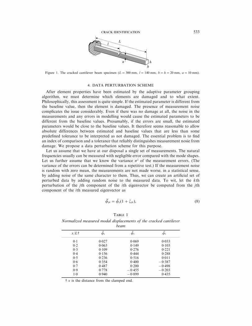
Figure 1. The cracked cantilever beam specimen (L=300 mm, l=140 mm, b= h=20 mm, a=10 mm).

4. DATA PERTURBATION SCHEME

After element properties have been estimated by the adaptive parameter groupingalgorithm, we must determine which elements are damaged and to what extent.Philosophically, this assessment is quite simple. If the estimated parameter is different fromthe baseline value, then the element is damaged. The presence of measurement noisecomplicates the issue considerably. Even if there was no damage at all, the noise in themeasurements and any errors in modelling would cause the estimated parameters to bedifferent from the baseline values. Presumably, if the errors are small, the estimatedparameters would be close to the baseline values. It therefore seems reasonable to allowabsolute differences between estimated and baseline values that are less than somepredefined tolerance to be interpreted as not damaged. The essential problem is to findan index of comparison and a tolerance that reliably distinguishes measurement nosie fromdamage. We propose a data perturbation scheme for this purpose.

Let us assume that we have at our disposal a single set of measurements. The naturalfrequencies usually can be measured with negligible error compared with the mode shapes.Let us further assume that we know the variance s2 of the measurement errors. (Thevariance of the errors can be determined from a repetitive test.) If the measurement noiseis random with zero mean, the measurements are not made worse, in a statistical sense,by adding noise of the same character to them. Thus, we can create an artificial set ofperturbed data by adding random noise to the measured data. To wit, let the kthperturbation of the jth component of the ith eigenvector be computed from the jthcomponent of the ith measured eigenvector as

f ijk =f ij(1+ zijk), (8)

T 1

Normalized measured modal displacements of the cracked cantileverbeam

x/L† f 1 f 2 f 3

0·1 0·027 0·069 0·0330·2 0·063 0·149 0·1030·3 0·109 0·276 0·2210·4 0·156 0·444 0·2880·5 0·236 0·516 0·0110·6 0·354 0·400 −0·3870·7 0·487 0·200 −0·4980·9 0·778 −0·455 −0·2031·0 0·940 −0·899 0·435

† x is the distance from the clamped end.

. . . 534

where zijk is a random variate with zero mean and variance s2. By carrying out the adaptiveparameter grouping algorithm M times, we generate a Monte Carlo sample of parameterestimates for each of the elements. We can take the mean value of the sample as theestimated parameter value, for each element. The standard deviation of the sample, foreach element, gives a measure of the sensitivity of that element to the measurement noise.

Let x*m represent the baseline value of the property associated with element m. Let x̄m

be the mean and sm the standard deviation of the Monte Carlo sample of estimates forelement m. Two damage indices can be defined to assist the damage detection andassessment process as follows:

bias–cxm ==x̄m − x*m =

x*m, bias–sdm =

=x̄m − x*m =sm

. (9, 10)

The first index, bias–cxm , indicates how close the averaged element parameter x̄m is to thebaseline value x*m . If the measurement noise is small and if the parameter value of elementm is reliably estimated, then bias–cxm will be a good indicator of damage. However, whenthe noise level is high or when the parameter value of element m is not well representedin the data, it may be difficult to reliably infer damage from bias–cxm . An insensitiveelement will generally exhibit a high variance in the Monte Carlo sample. Thus, bias–sdm

can be used to reduce the risk of identifying an actually undamaged element as a damagedone. It is possible for bias–sdm to become a large value when sm is small compared with=x̄m − x*m = due to an excellent estimation. Therefore, the two damage indices must be usedtogether to detect damage in a structural system.

Let cxlmt and sdlmt be the threshold values of bias–cx and bias–sd, respectively. Wewill consider an element damaged if

bias–cxm q cxlmt AND bias–sdm q sdlmt. (11)

The threshold values of the two damage indices must be determined to optimallydistinguish measurement noise from damage. These values can be estimated from a MonteCarlo simulation of the baseline structure. At the given noise level, cxlmt and sdlmt arethose values that predict no damage in all elements, say, 97% of the time. Damage canoften change the behavior of the structure a great deal. One may wish to repeat the MonteCarlo simulation on the identified damaged structure, as an a posteriori estimate, to assessthe efficacy of the values chosen from the baseline study. In the following case study wewill demonstrate the overall procedure of damage detection.

5. CRACK IDENTIFICATION CASE STUDY

In this section our damage assessment algorithm is used to locate and assess the severityof the crack in the cantilever beam shown in Figure 1. The modal responses were obtainedexperimentally by Rizos et al. [10]. They measured natural frequencies and modaldisplacements of a cantilever structure with a transverse surface crack extending uniformlyalong the width. The 300 mm cantilever with square cross-section 20 mm ×20 mm wasclamped to a vibrating table. Resonant harmonic excitation was applied and each of threemodes was investigated independently. Even though they tested various cases withdifferent crack locations and different crack depths, they documented the measurementsappropriate to our damage detection scheme for the case with the crack depth a=10 mmand the crack located at l=140 mm from the clamped end, as shown in Figure 1. Thecrack was initiated with a thin saw cut and propagated to the desired depth by fatigueloading. The crack depth was measured directly and verified with an ultrasonic detectorfor uniformity and actual depth of the crack.

535

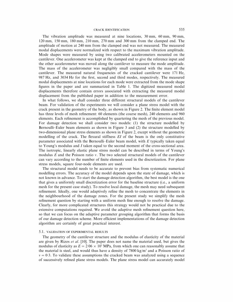
The vibration amplitude was measured at nine locations, 30 mm, 60 mm, 90 mm,120 mm, 150 mm, 180 mm, 210 mm, 270 mm and 300 mm from the clamped end. Theamplitude of motion at 240 mm from the clamped end was not measured. The measuredmodal displacements were normalized with respect to the maximum vibration amplitude.Mode shapes were measured by using two calibrated accelerometers mounted on thecantilever. One accelerometer was kept at the clamped end to give the reference input andthe other accelerometer was moved along the cantilever to measure the mode amplitude.The mass of the accelerometer was negligibly small compared with the mass of thecantilever. The measured natural frequencies of the cracked cantilever were 171 Hz,987 Hz, and 3034 Hz for the first, second and third modes, respectively. The measuredmodal displacements at nine locations for each mode were extracted from the mode shapefigures in the paper and are summarized in Table 1. The digitized measured modaldisplacements therefore contain errors associated with extracting the measured modaldisplacement from the published paper in addition to the measurement error.

In what follows, we shall consider three different structural models of the cantileverbeam. For validation of the experiments we will consider a plane stress model with thecrack present in the geometry of the body, as shown in Figure 2. The finite element modelhas three levels of mesh refinement: 60 elements (the coarse mesh), 240 elements and 960elements. Each refinement is accomplished by quartering the mesh of the previous model.For damage detection we shall consider two models: (1) the structure modelled byBernoulli–Euler beam elements as shown in Figure 3 and (2) the structure modelled bytwo-dimensional plane stress elements as shown in Figure 2, except without the geometricmodelling of the crack. The flexural stiffness EI of the beam is the only constitutiveparameter associated with the Bernoulli–Euler beam model, with E typically taken equalto Young’s modulus and I taken equal to the second moment of the cross-sectional area.The isotropic, linearly elastic plane stress model can be described in terms of Young’smodulus E and the Poisson ratio n. The two selected structural models of the cantilevercan vary according to the number of finite elements used in the discretization. For planestress models, square four-node elements are used.

The structural model needs to be accurate to prevent bias from systematic numericalmodelling errors. The accuracy of the model depends upon the state of damage, which isnot known in advance. To start the damage detection algorithm, the best model is the onethat gives a uniformly small discretization error for the baseline structure (i.e., a uniformmesh for the present case study). To resolve local damage, the mesh may need subsequentrefinement. Ideally, one would adaptively refine the mesh to concentrate the elements inthe neighbourhood of the damage zones. For the present study we simplify the meshrefinement question by starting with a uniform mesh fine enough to resolve the damage.Clearly, for more complicated structures this strategy would not be practical due to theextensive computations required. We avoid the adaptive mesh refinement question here,so that we can focus on the adaptive parameter grouping algorithm that forms the basisof our damage detection scheme. More efficient implementations of the damage detectionalgorithm are certainly of great practical interest.

5.1.

The geometry of the cantilever structure and the modulus of elasticity of the materialare given by Rizos et al. [10]. The paper does not name the material used, but gives themodulus of elasticity as E=2·06×105 MPa, from which one can reasonably assume thatthe material is steel, and would thus have a density of 7800 kg/m3 and a Poisson ratio ofn=0·3. To validate these assumptions the cracked beam was analyzed using a sequenceof successively refined plane stress models. The plane stress model can accurately model

514631266

Measurement locations

11 16 21 36

L = 300 mm

140 mm

. . . 536

Figure 2. The structural model with 50 Bernoulli–Euler beam elements.

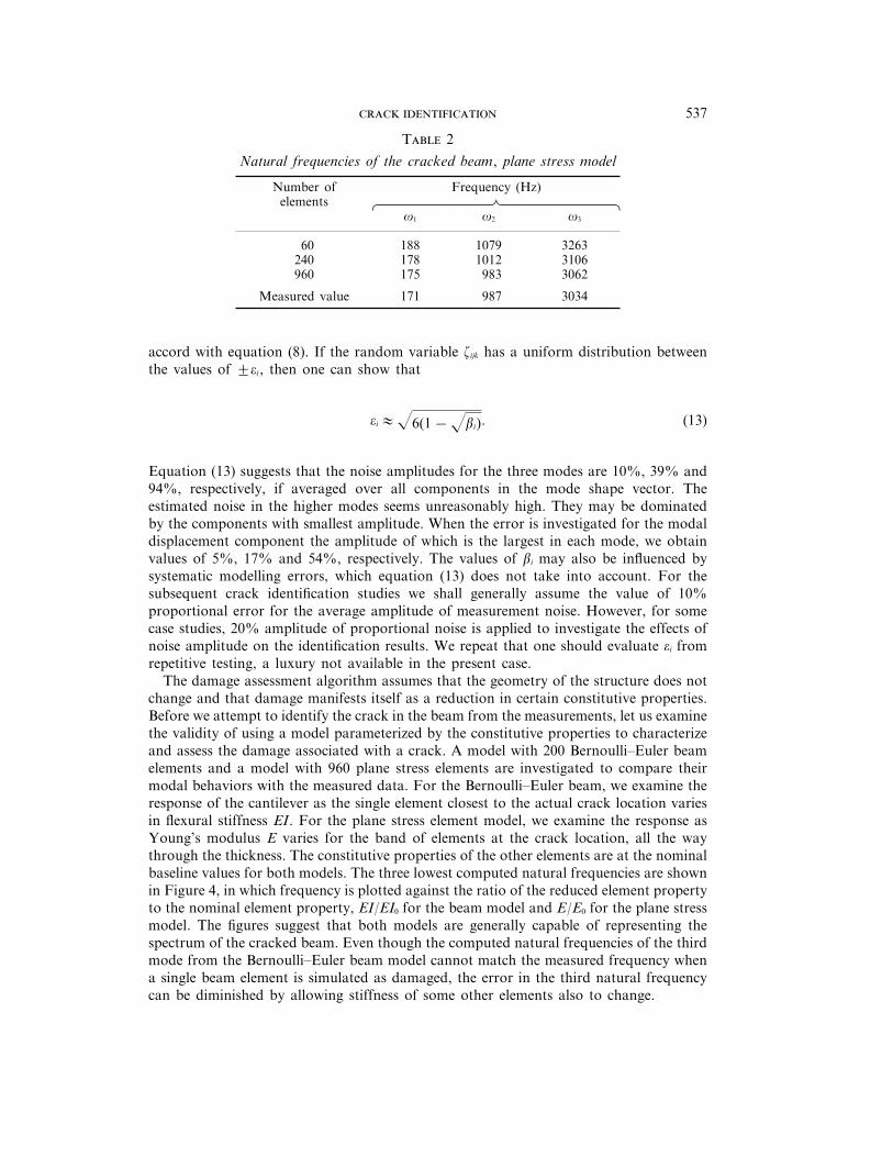
the geometry of the cracked beam, unlike the Bernoulli–Euler beam model. The threelowest computed natural frequencies from 60-, 240- and 960-element meshes aresummarized in Table 2. From the table, we can observe that the computed frequenciesdiffer from the measured data by less than 2% when 960 elements are used. The closecorrespondence between measurements and model suggest that the properties andgeometry used in the model closely reflect the features of the experiment.

The results in Table 2 also show that the less refined models predict natural frequencieshigher than the measured values for all the three modes. Despite the fact that these modelsare not completely accurate, we shall demonstrate that they are still useful for the problemof damage detection. The error in frequency will be distributed across the structure as areduction in element stiffness by the parameter estimation algorithm, rather than as localchanges in element properties, and will not necessarily mask the real damage. The questionof how accurate the finite element model needs to be to minimize the affects of thesesystematic modelling errors is problem dependent, but can always be addressed by a meshrefinement study.

The amplitude of noise in the measured modal displacements is needed in the damageassessment algorithm. Typically, this information would be available from a baselineevaluation of the undamaged structures. No baseline measurements are available for thecurrent problem. However, since the exact crack location and depth are given from theexperiment by Rizos et al. [10], the missing information may be deduced from theanalytical study of the cracked beam. The error in the modal displacement is thecombination of the actual sensor error and the error that we committed in digitizing thedata from the original paper. To quantify the error between the analytical mode shape andthe measured mode shape, we employ the well-known modal assurance index.

bi 0(c i · f i)2

>c i>2>f i>2, (12)

where c i and f i are the ith analytical and measured mode shapes, respectively, with onlythe measurement locations included. Clearly, when the analytical mode shape is close tothe measured shape, the value of bi is close to unity. The discrepancy between the computedand measured modes for the three different plane stress models is summarized in Table 3.From the table, one can observe that the error increases with the mode number, but theerrors do not change with refinement of the finite element mesh. There is a considerabledifference between the third mode shape predicted by the finite element model and the onemeasured.

The amplitude of measurement noise can be deduced from the modal assurance indexif one assumes that errors are random and proportional to the measurement value, in

Figure 3. The structural model with plane elements (coarse mesh).

537

T 2

Natural frequencies of the cracked beam, plane stress model

Frequency (Hz)Number ofZxxxxxxxCxxxxxxxVelements

v1 v2 v3

60 188 1079 3263240 178 1012 3106960 175 983 3062

Measured value 171 987 3034

accord with equation (8). If the random variable zijk has a uniform distribution betweenthe values of 2oi , then one can show that

oi 1z6(1−zbi). (13)

Equation (13) suggests that the noise amplitudes for the three modes are 10%, 39% and94%, respectively, if averaged over all components in the mode shape vector. Theestimated noise in the higher modes seems unreasonably high. They may be dominatedby the components with smallest amplitude. When the error is investigated for the modaldisplacement component the amplitude of which is the largest in each mode, we obtainvalues of 5%, 17% and 54%, respectively. The values of bi may also be influenced bysystematic modelling errors, which equation (13) does not take into account. For thesubsequent crack identification studies we shall generally assume the value of 10%proportional error for the average amplitude of measurement noise. However, for somecase studies, 20% amplitude of proportional noise is applied to investigate the effects ofnoise amplitude on the identification results. We repeat that one should evaluate oi fromrepetitive testing, a luxury not available in the present case.

The damage assessment algorithm assumes that the geometry of the structure does notchange and that damage manifests itself as a reduction in certain constitutive properties.Before we attempt to identify the crack in the beam from the measurements, let us examinethe validity of using a model parameterized by the constitutive properties to characterizeand assess the damage associated with a crack. A model with 200 Bernoulli–Euler beamelements and a model with 960 plane stress elements are investigated to compare theirmodal behaviors with the measured data. For the Bernoulli–Euler beam, we examine theresponse of the cantilever as the single element closest to the actual crack location variesin flexural stiffness EI. For the plane stress element model, we examine the response asYoung’s modulus E varies for the band of elements at the crack location, all the waythrough the thickness. The constitutive properties of the other elements are at the nominalbaseline values for both models. The three lowest computed natural frequencies are shownin Figure 4, in which frequency is plotted against the ratio of the reduced element propertyto the nominal element property, EI/EI0 for the beam model and E/E0 for the plane stressmodel. The figures suggest that both models are generally capable of representing thespectrum of the cracked beam. Even though the computed natural frequencies of the thirdmode from the Bernoulli–Euler beam model cannot match the measured frequency whena single beam element is simulated as damaged, the error in the third natural frequencycan be diminished by allowing stiffness of some other elements also to change.

. . . 538

5.2. –

Let us turn our attention to the problem of identifying the location of the crack usinga Bernoulli–Euler beam model. Since we assume no knowledge of the crack location inadvance, it is most logical to discretize the cantilever beam with equal sized elements. Thefinite element model does not change during the damage localization process, so it isimportant to begin with a suitably fine mesh at the outset. For the current study, we usea model with 50 Bernoulli–Euler beam elements. Although 50 elements is far more thanrequired to reduce the finite element discretization error, this refinement is necessary toaccurately resolve the damage. The data perturbation iterations are executed 50 times,which is adequate to establish statistical significance of the estimates.

The Bernoulli–Euler beam element has a single constitutive parameter, the flexuralstiffness EI. Damage is inferred as a reduction in the flexural stiffness of an element orgroup of elements. Since the number of measured modal displacement for each node N d

is equal to nine and the number of measured modes Nm is equal to three, the limit to thenumber of unknown parameters in the model N0 is 27, according to equation (5). Sincethe member properties of the uncracked baseline cantilever structure can be assumed tobe uniform over the whole length of the structure, the number of parameter groups startswith Np =1. Subdivision can continue up to a maximum of 27 groups.

Before evaluating the cracked cantilever structure, it is necessary to determine the upperlimit values for the damage indices from a simulation study of the baseline structure. Thedetermined upper limit values cxlmt and sdlmt for damage indices bias–cx and bias–sd,respectively, will be used to discern damage from noise in each element. In Figure 5(a) areshown the mean and standard deviation of the parameter estimates of the baselinestructure (no crack) over 50 Monte Carlo trials with 10% imposed noise. One can see thatthe elements at the tip of the cantilever beam are the most influenced by noise. Theprobability of detecting each member as damaged as a function of the sdlmt value is shownin Figure 5(b). There is a curve plotted for each element, with the ordinate giving thepercentage of times the member was identified as damaged in the Monte Carlo sample forthe given sdlmt value. One can see that for values of sdlmt less than 1, many of the membersare detected as damaged, some of them quite often, even though there is no damage.Therefore, an appropriate value of sdlmt for damage detection is 1·1. For this value ofsdlmt no member in the baseline structure is detected as damaged in more than 3% of theMonte Carlo trials. One can do the same exercise to determine cxlmt, but in this case thestructure is not sensitive to cxlmt. Shin and Hjelmstad [17] have suggested setting cxlmtequal to the noise amplitude, 10% in the present case.

Now let us try to locate the crack in the damaged structure. In Figure 6(a) are shownthe computed mean and standard deviation values of flexural stiffnesses of the damagedstructure, as determined from the 50 data perturbation iterations. The damage indices are

T 3

Computed modal displacement errors, plane stress model

Modal assurance indexNumber ofZxxxxxxxCxxxxxxxVelements

b1 b2 b3

60 0·996 0·956 0·729240 0·996 0·953 0·729960 0·997 0·951 0·730

0.2

200

1500.0

Fre

quen

cy (

Hz) 190

180

170

160

0.1

(a)

0.2

1200

7000.0

Stiffness ratio

1100

1000

900

800

0.1

(b)

0.2

3300

29000.0

3200

3100

3000

0.1

(c)

3000

Fle

xura

l sti

ffn

ess

2500

1000

500

(a)

Element ID number

2000

1500

2

40

0

Dam

age

prob

abil

ity

(%)

20

10

(b)

sdlmt

30

1

01 8 15 5022 29 36 43

539

Figure 4. Variation of the natural frequencies with respect to the stiffness ratio for (a) the first mode; (b) thesecond mode and (c) the third mode. ——, Measured value; W, Bernoulli–Euler beam model; R, plane stressmodel.

shown in Figure 6(b). The bias–sd values of elements 1–25 are rather large, but the bias–cxvalues are less than cxlmt. Hence, these elements are not detected as damaged. Element26 is clearly identified as damaged. It is quite near the actual crack. With cxlmt=10%and sdlmt=1·1, elements 31 and 46 are also detected as damaged. This anomalous resultis worth noting, and is indicative of the problem of identifying a crack with aBernoulli–Euler beam model.

The fact that we very nearly detected all of members 1–25 as damaged deserves furtherexamination. In Figure 7 are shown the computed natural frequencies of the damagedcantilever beam from three different estimated models. In case (i) we set EI of element 26equal to its estimated values but all others at their nominal values. In case (ii) we set EIof elements 26, 31 and 46 equal to their estimated values with all others at their nominalvalues. In case (iii) we set EI of all elements equal to their estimated values. Case (i) matchesthe first frequency very well, but has difficulty with the second and third. Thus, changingelement 26 gets us fairly close to the measured response. The changes in parameters in theother elements are needed to match the higher modes more closely. This problem is anartifact of the inability of the Bernoulli–Euler beam to capture the spectrum of the crackedbeam noted earlier. The estimated parameters will attempt to make up for shortcomingsin the model, often to the detriment of damage detection. The mode shapes for case (i)

Figure 5. (a) The mean and standard deviation of the estimated flexural stiffnesses from the Monte Carlosample: ——, baseline; W, mean; R, standard deviation. (b) The variation of the damage probability with respectto sdlmt for the baseline structure for cxlmt=10%.

50

3000

01

Fle

xura

l sti

ffn

ess

2500

1000

500

8

(a)

Element ID number

2000

1500

15 22 29 36 43

50

15

0

(b)

Element ID number1 8 15 22 29 36 43

105

60

01020304050

100

0

bias

–sd

20

40

501 8 15 22 29 36 43

60

80

bias

–sd

bias

–sd

300

0

Fre

quen

cy (

Hz)

100

(i)

(a)

200

(ii) (iii)

1150

850

950

(i)

1050

(ii) (iii)

3300

3000

3100

(i)

(c)

3200

(ii) (iii)

(b)

. . . 540

Figure 6. Damage localization and assessment with the 50 Bernoulli–Euler beam element model. (a) Parameterestimates and standard deviations from perturbation iterations: ——, base line; W, mean; R, standard deviation.(b) Damage indices for each element.

are compared with the measured data in Figure 8. The mode shapes from the other twocases also yielded roughly the same results.

One of the primary interests of the current study is to investigate how well aBernoulli–Euler beam model can locate the crack and assess damage by a reduced flexuralstiffness. In Figure 9, the results from three different Bernoulli–Euler beam models with20, 30 and 50 beam elements are compared. For the purpose of comparison, the locationof a crack is defined as the distance from the fixed end to the middle of the element whichwas detected as the most highly damaged. The estimated flexural stiffness of the detectedelement is also compared in the same figure. We can observe that the identified cracklocation approaches the actual cracked section as a more refined beam model is applied.As more elements are used, flexural stiffness of the element identified as damaged reducesrapidly because the length of the damaged element decreases.

Figure 7. Computed natural frequencies with reduced flexural stiffness in different elements; cases (i), (ii) and(iii) for (a) the first mode, (b) the second mode and (c) the third mode. The solid horizontal line represents themeasured value.

1

–1

0

0.0

(c)

0.2 0.4 0.6 0.8 1.0

x/L

1

–1A

mpl

itu

de

0

(b)

1

0

(a)

300

0

100

(a)

20 30 40 50 60

Number of beam elements

Cra

ck lo

cati

on

10

50

150200250

1200

0

(b)

20 30 40 50 60

Fle

xura

l sti

ffn

ess

10

300

600

900

541

Figure 8. The computed lowest three mode shapes of the Bernoulli–Euler beam model with 50 elements whenthe flexural stiffness of element 26 is reduced with (a) the first mode, (b) the second mode and (c) the third mode.——, Identified; W, measured.

We have repeated the analysis of the cracked beam using Timoshenko beam elements.The results, presented in detail in reference [17], are omitted here for the sake of brevity.The Timoshenko beam element has twice as many constitutive parameters as theBernoulli–Euler beam. Consequently, the advantages gained by accounting for sheardeformation in the vibration frequencies and mode shapes are counteracted by the relativeloss of information content in the data. That observation notwithstanding, the results ofthe Timoshenko beam model are qualitatively similar to those of the Bernoulli–Euler beammodel, leading us to conclude that the performance of these two models is dominated bythe one-dimensional nature of the approximation rather than the importance of shear.

5.3.

For a plane stress model, there are two constitutive parameters in each element, Young’smodulus E and the Poisson ratio n. By modelling the cantilever with plane stress elements,one can capture many physical features of the cracked beam that the Bernoulli–Eulermodel precluded. For example, shear deformation becomes important in studying themodes of vibration of higher frequencies [20]. Also, the stress concentration effects of acrack can be represented by a plane stress model.

Figure 9. The estimated crack location (a) and the flexural stifiness of the cracked element (b). ——, Actualcrack location; W, estimated crack location.

5000

1000

(b)

Eb

Element ID number

200030004000

5000

01000

(a)200030004000

10

0

(c)

0.5 1.0Dam

age

prob

abil

ity

(%)

sdlmt

5

0 10 20 30 40 6050

. . . 542

Figure 10. The mean and standard deviation of E from the Monte Carlo sample for (a) top elements and (b)bottom elements: ——, baseline; W, mean; R, standard deviation. (c) Variation of the damage probability withrespect to sdlmt for the baseline structure for cxlmt=10%.

When there are more than two parameters per element, it may be that they are notequally represented in the data. In the plane stress problem, the Poisson ratio is typicallydifficult to estimate from the given (transverse displacement) measurements because it isnot sensitive to them. In a simulation study of the cantilever beam, we observed thatestimated values of the Poisson ratio hit the upper or lower bounds frequently during theidentification processes, while Young’s modulus was more robustly estimated. To generatean alternate measurement set, we used a 960-element plane stress model. Those data werethen used with a 60-element plane stress model for damage detection. Estimating twoparameters in each element, we found that the estimates of the Poisson ratio were notreliable for locating damage in the structure, while Young’s modulus estimates were. Wetherefore consider the Poisson ratio for all elements to be fixed at the nominal value forall of the subsequent studies. A model with 60 plane stress elements is selected to carryout damage detection on the cantilever structure. The initial number of parameter groupsstarts from one because the stiffness properties of the uncracked baseline cantileverstructure can be assumed to be uniform over the whole structure.

The upper limit values for the damage indices are determined by the damage probabilitycurves obtained from a simulation study of the baseline structue as shown in Figure 10.Mean and standard deviations from the Monte Carlo sample for the baseline structure arealso shown. From the figure, one can observe that most of the elements are sensitiveenough with respect to the test conditions with their small standard deviations, eventhough the elements near the free end show a little higher standard deviation values. Fromthe damage probability figure, we can determine the upper limit values as sdlmt=0·48 andcxlmt=10% (equal to the noise amplitude).

The computed mean and standard deviation values and the damage indices for eachelement compiled in Figure 11, from 50 data perturbation iterations. From the figure, the

5000

0

1000

(b)

10 20 30 40 60

Eb

50Element ID number

200030004000

80

0

(e)

10 60

bias

–cx

(%)

Element ID number

40

5000

01000

(a)200030004000

4020 30 50

20

60

80(c)

bias

–cx

(%)

4020

60

800

0

(f)

10 60

bias

–sd

Element ID number

400

4020 30 50

200

600

800

0

(d)

bias

–sd

400200

600

0

543

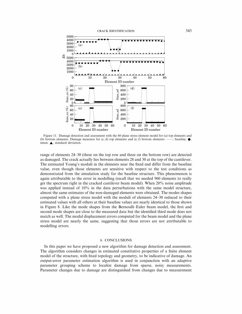
Figure 11. Damage detection and assessment with the 60 plane stress element model for (a) top elements and(b) bottom elements. Damage measures for (c, d) top elements and (e, f) bottom elements. ——, baseline; W,mean; R, standard deviation.

range of elements 24–30 (three on the top row and three on the bottom row) are detectedas damaged. The crack actually lies between elements 28 and 30 at the top of the cantilever.The estimated Young’s moduli in the elements near the fixed end differ from the baselinevalue, even though those elements are sensitive with respect to the test conditions asdemonstrated from the simulation study for the baseline structure. This phenomenon isagain attributable to the error in modelling (recall that we needed 960 elements to reallyget the spectrum right in the cracked cantilever beam model). When 20% noise amplitudewas applied instead of 10% in the data perturbations with the same model structure,almost the same estimates of the non-damaged elements were obtained. The modes shapescomputed with a plane stress model with the moduli of elements 24–30 reduced to theirestimated values with all others at their baseline values are nearly identical to those shownin Figure 8. Like the mode shapes from the Bernoulli–Euler beam model, the first andsecond mode shapes are close to the measured data but the identified third mode does notmatch as well. The modal displacement errors computed for the beam model and the planestress model are nearly the same, suggesting that those errors are not attributable tomodelling errors.

6. CONCLUSIONS

In this paper we have proposed a new algorithm for damage detection and assessment.The algorithm considers changes in estimated constitutive properties of a finite elementmodel of the structure, with fixed topology and geometry, to be indicative of damage. Anoutput-error parameter estimation algorithm is used in conjunction with an adaptiveparameter grouping scheme to localize damage from sparse, noisy measurements.Parameter changes due to damage are distinguished from changes due to measurement

. . . 544

noise with a data perturbation scheme. The limiting values for the two statistical damageindices are established through a Monte Carlo simulation of the baseline structure. Oneof the advantages of the algorithm presented here is that the sensitivity of each elementparameter can be evaluated during the process of the damage detection. The sensitivityof the element parameters need not be determined separately before trying to detectdamage in the structure.

The damage detection algorithm was applied to the problem of identifying a crack ina cantilever beam. The measured data for the cracked beam were taken from the literature.All aspects of the damage detection scheme were examined except for establishing thebaseline parameters from measurements, which were not available among the reportedresults. (We considered the baseline model to be adequately described by the nominaldimensions and properties of the beam.) The Bernoulli–Euler beam model identified thecrack, but also suggested damage at other locations along the beam. Analysis showed thatthe kinematic constraints associated with the beam theory caused difficulties in matchingthe response of the higher frequency modes when only the beam modulus EI was availableto adapt to the measurements. A reduced bending modulus is only a marginally effectiveway of modelling a crack in a beam. (Beam theory with a crack element as in reference[10] that explicitly models the geometric defect does not suffer from this problem.) Theplane stress model gave much better results, giving a reliable and accurate assessment ofthe crack location. Thus, one can conclude that using a change in element constitutiveproperties is a reasonable approach to the problem of detecting topological damage likecracks. Furthermore, the mesh refinement required to detect damage is relatively modest.The 60-element model proved adequate to detect damage even though the 60-elementmodel with the crack explicitly modelled showed errors in frequency of the order of 10%.

It seems intuitively clear that the smeared crack approach cannot do better than anapproach that geometrically models the crack because the singularity in the strain fieldassociated with the crack is very important. In particular, all other things being equal, oneshould expect the estimates from the crack element approach [10] to be sharper than thoseobtained here. However, identification of geometric features of a solid body in general isinherently more difficult than identification of constitutive parameters. In the case studyexamined here there was a single vertical crack in the beam. In a practical application wemay not have such knowledge. The strength of the present approach lies in its generality.We need know nothing about the damage (e.g., that it even manifests as a crack) beforewe begin our assessment of it. The method can adapt to a variety of defects withoutrequiring a reformulation. We have shown that this general approach has merit in thecontext of the difficult problem of crack identification.

ACKNOWLEDGMENT

The research reported here was supported by the National Science Foundation undera Presidential Young Investigator Award. The results, opinions and conclusions expressedin the paper are solely those of the writers and do not necessarily represent those of thesponsors.

REFERENCES

1. M. S. A, S. F. M, R. K. M and T. K. C 1991 Journal of EngineeringMechanics, American Society of Civil Engineers 117, 370–390. System identification approachto detection of structural changes.

545

2. P. H and F. J. S 1990 American Institute of Aeronautics and Astronautics Journal 28,1110–1115. Structural damage detection based on static and modal analysis.

3. F. I, A. I and H. R. M 1990 Journal of Sound and Vibration 140, 305–317.Identification of fatigue cracks from vibration testing.

4. T. Y. K and T. Y. L 1994 International Journal of Solids and Structures 31, 925–940. Cracksize identification using an expanded mode method.

5. T. W. L and T. A. L. K 1994 American Institute of Aeronautics and AstronauticsJournal 32, 1049–1057. Structural damage detection of space truss structures using bestachievable eigenvectors.

6. H. G. N 1989 ’89, Politechnike Pozuanska, 99–110. Identification approachesin damage detection and diagnosis.

7. H. G. N and C. C 1991Mathematical Systems and Signal Processing 5, 345–356. Faultdetection and localization in structures: A discussion.

8. A. K. P, M. B and M. M. S 1991 Journal of Sound and Vibration 145,321–332. Damage detection from changes in curvature mode shape.

9. J. M. R and J. B. K 1992 American Institute of Aeronautics and AstronauticsJournal 30, 2310–2316. Damage detection in elastic structures using vibratory residual forces andweighted sensitivity.

10. P. F. R, N. A and A. D. D 1990 Journal of Sound and Vibration 138,381–388. Identification of crack location and magnitude in a cantilever beam from the vibrationmodes.

11. N. S, T. H. B and R. O 1990 International Journal of Analytical andExperimental Modal Analysis 5, 67–79. Global non-destructive damage evaluation in solids.

12. D. C. Z and M. K 1992 American Institute of Aeronautics and AstronauticsJournal 30, 1848–1855. Eigenstructure assignment approach for structural damage detection.

13. D. J. E 1984 Modal Testing: Theory and Practice. New York: John Wiley.14. J. W 1990 Applied Mechanics Reviews 43, 13–17. On the dynamics of cracked rotors: a

literature survey.15. K. D. H, M. R. B and M. R. B 1995 Earthquake Engineering and Structural

Dynamics 24, 53–67. On building finite element models of structures from modal response.16. K. D. H, S. L. W and S. J. C 1992 Journal of Structural Engineering, American

Society of Civil Engineers 118, 223–242. Mutual residual energy method for parameter estimationin linear structures.

17. S. S and K. D. H 1994 Structural Research Series Report No. 593,UILU-ENG-94-2013, Department of Civil Engineering, University of Illinois at Urbana–Cham-paign. Damage detection and assessment of structural systems from measured response.

18. A. R. B 1984 in Self-organizing Methods in Modelling (S. J. Falow, editor). New York:Marcel Dekker. Predicted squared error: a criterion for automatic model selection.

19. H. A 1972 in Proceedings of the 2nd International Symposium on Information Theory (B. N.Petrov and F. Csaki, editors), 267–281. Budapest: Akademiai Kiado. Information theory andan extension of the maximum likelihood principle.

20. S. T, D.H. Y and W. W, J. 1974 Vibration Problems in Engineering NewYork: John Wiley; fourth edition.