1968 Risk, Return and Equilibrium Some Clarifying Comments

8/13/2019 1968 Risk, Return and Equilibrium Some Clarifying Comments

http://slidepdf.com/reader/full/1968-risk-return-and-equilibrium-some-clarifying-comments 1/12

RISK, RETURN AND EQUILIBRIUM: SOME CLARIFYING

COMMENTS

EUGENE F. F M

SH RPE [12] ND LINTNER [7] have recently proposed models directed at

the following questions: a What is the appropriate measure of the risk ofa capital asset? b What is the equilibrium relationship between this measureof the asset's risk and its one-period expected returnr Lintner contends thatthe measure of risk derived from his model is different and more general than

that proposed by Sharpe. In his reply to Lintner, Sharpe [13] agrees thattheir results are in some ways conflicting and that Lintner's paper supersedeshis.

This paper will show that in fact there is no conflict between the SharpeLintner models. Properly interpreted they lead to the same measure of therisk of an individual asset and to the same relationship between an asset'srisk and its one-period expected return. The apparent conflicts discussed bySharpe and Lintner are caused by Sharpe's concentration on a special stochasticprocess for describing returns that is not necessarily implied by his asset

pricing model. 'When applied to the more general stochastic processes thatLintner treats, Sharpe's model leads directly to Lintner's conclusions.

I. EQUILmRIUM IN THE SH RPE MODEL

The Sharpe capital asset pricing model is based on the following assumptions: a The market for capital assets is composed of risk averting investors,

all of whom are one-period expected-utility-of-terminal-wealth maximizers (inthe von Neumann-Morgenstern [16] sense) and find it possible to make

optimal portfolio decisions solely on the basis of the means and standarddeviations of the probability distributions of terminal wealth associated withthe various available portfolios. the one-period return on an asset or portfolio is defined as the change in wealth during the horizon period divided by

the initial wealth invested in the asset or portfolio, then the assumption implies

Associate Professor of Finance, Graduate School of Business, University of Chicago. preparing this paper I have benefited from discussions with members of the Workshop in Financeof the Graduate School of Business. The comments of M. Blume, P. Brown, M. Jensen, M.Miller, H. Roberts, R. Roll, M. Scholes and A. Zellner were especially helpful. The research was

supported by a grant from the Ford Foundation.1. The terms capital asset and one-period return will be defined below.

2. In the one-period expected utility of terminal wealth model, the objects of choice for theinvestor are the probability distributions of terminal wealth provided by each asset and portfolio.Each portfolio represents a complete investment strategy covering all assets (e.g., bonds, stocks,insurance, real estate, etc.) that could possibly affect the investor's terminal wealth. That is, atthe beginning of the borizon period the investor makes a single portfolio decision concerning theallocation of his investable wealth among the available terminal wealth producing assets. ADterminal wealth producing assets are called capital assets.





a R

o

Risk Return and quilibrium

1 ~ 1A

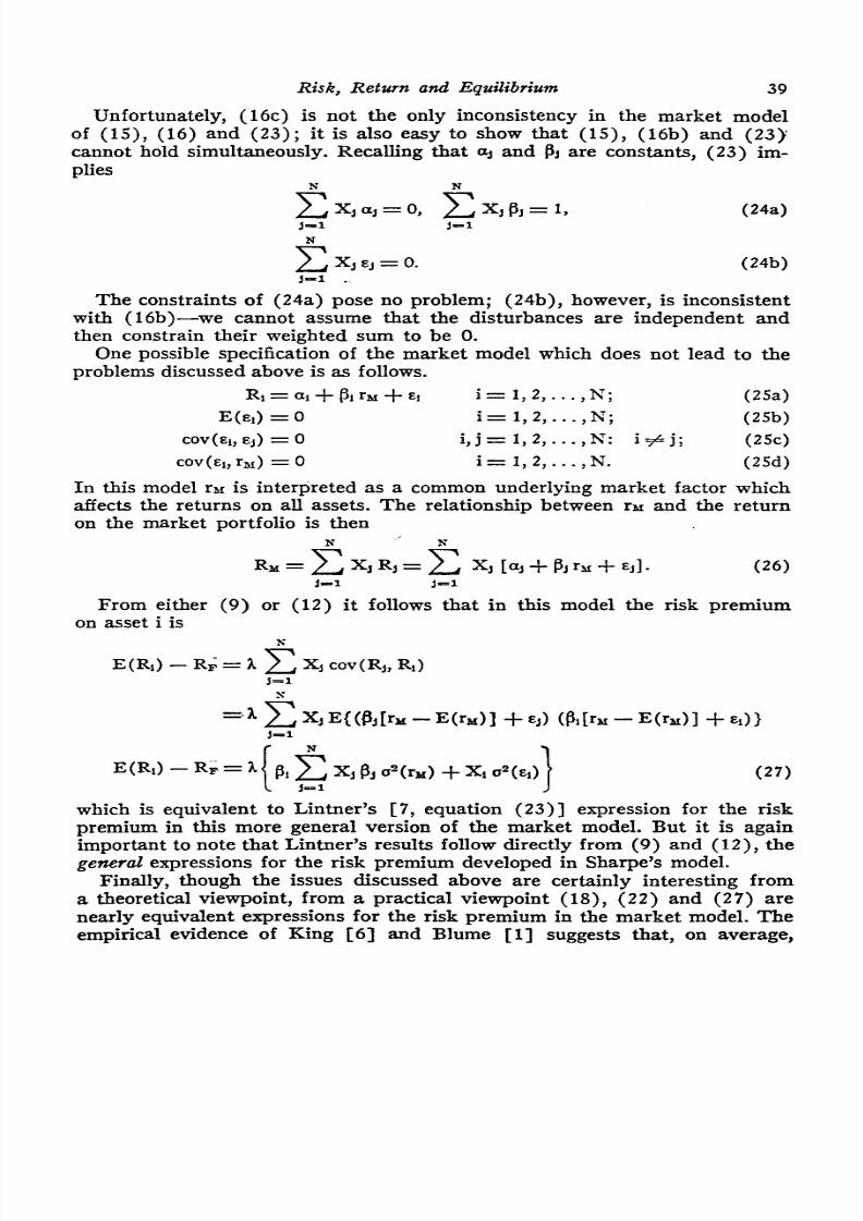
FIGURE 1

z

31

Assumptions b , (c) and (d) of the Sharpe model standardize the pictureof the portfolio opportunity set available to each investor. Assumption b implies that the portfolio decisions of all investors are made at the same pointin time, and the horizon considered in making these decisions is the same forall. Assumptions (c) and d standardize both the set of available portfolios

and investors evaluations of the combinations of expected return and standarddeviation provided by each member of the set,The situation facing each investor can be represented as in Figure 1. The

horizontal axis of the figure measures expected return E R over the commonhorizon period, while the vertical axis measures standard deviation of return,a R . attention is restricted to portfolios involving only risky assets,Sharpe [12] shows that the set of mean-standard deviation efficient portfolioswill fall along a curve convex to the origin, like LMO in Figure 1.8

7. Lintner [7, pp, 600-01] considers an extension of the asset pricing model to the case where

investors disagree on the expected returns and standard deviations provided by portfolios. Theresults are essentially the same as those derived under the assumption of homogenous expectations. Since Lintner s criticism of Sharpe does not depend on this part of his work, our discussion will use the simpler homogeneous expectations version of the model. Most of Lintner sdiscussion is also within this framework, and in all other respects his assumptions are identical tothose of Sharpe.

It is important to emphasize that the Sharpe-Lintner asset pricing models, like the MarkowitzTobin portfolio models, present one-period analyses. For a more complete discussion of the onperiod framework see [4].

8. Strictly speaking this result presupposes that there are at least two portfolios in the efficientset. That is, there is no portfolio which has both higher expected return and lower standard devia-



32 h ournal of inance

The model assumes, however, that in addition to the opportunities presentedby portfolios of risky assets, there is a riskless asset F which will provide the

sure return RF over the common horizon period; it is assumedthat

the investorcan both borrow and lend at the riskless rate RF. Consider portfolios C involving combinations of the riskless asset F and an arbitrary portfolio A ofrisky assets. The expected return and standard deviation of return providedby such combinations are

E Re = x RF + 1 - x) E RA

a Re = 1 - x) a RA

1, 1

2

3

where x is the proportion of available funds invested in the riskless asset F,

so that l-x is invested in A. Applying the chain rule,d a Re d a Re dx a RA

d E Re dx d E Re E RA - RF

This implies that the combinations of expected return and standard deviationprovided by portfolios involving F and A must fall along a straight line throughRF and A in Figure 1.

t is now easy to determine the effects of borrowing-lending opportunitieson the set of efficient portfolios. In Figure 1 consider the line RFMZ, touch

ing LMO at M. This line represents the combinations of expected return andstandard deviation associated with portfolios where the proportion x x 1)is invested in the riskless asset F and 1-x in the portfolio of risky assets M.At the point RF, x = 1, while at the point M, x = Points below M alongRFMZ correspond to lending portfolios x> 0 , while points above Mcorrespond to borrowing portfolios x < 0 . At given levels of a R there areportfolios along RFMZ which provide higher levels of E R than the corresponding portfolios along LMO. Thus except for M the portfolios alongLMO are dominated by portfolios along RFMZ, which is now the efficient set.

The conditions necessary for equilibrium in the asset market can now bestated. Since all investors have the same horizon and view their portfolioopportunities in the same way, the Sharpe model implies that everybody facesthe same picture of the set of efficient portfolios. the relevant picture isFigure 1, then all efficient portfolios for all investors will lie along RFMZ.More risky efficient portfolios involve borrowing x < 0) and investing allavailable funds including borrowings) in the risky combination M. Lessrisky efficient portfolios involve lending x 0) some funds at the rate RFand investing remaining funds in M. The particular portfolio that an investor

chooses will depend on his attitudes toward risk and return, but optimumportfolios for all investors will involve some combination of the riskless assetF and the portfolio of risky assets M There will be no incentive for anyone

tion of return than any other portfolio. In a market of risk averters with homogeneous expectations this is not a strong presumption.

9. As noted earlier, Tobin [15] shows that the mean-standard deviation portfolio model isappropriate either when probability distributions of returns on portfolios are normal or wheninvestor utility of return functions are well approximated by quadratics. In either case the indifference curves I.e., loci of constant expected util ity) of a risk averter will be positively sloping



Risk Return and Equilibrium 33

to hold risky assets not included in M. M does not contain all the riskyassets in the market, or if it does not contain them in exactly the proportionsin which they are outstanding, then there will be some assets that no one willhold. This is inconsistent with equilibrium, since in equilibrium all assets mustbe held.

Thus, Figure 1 is to represent equilibrium, M must be the market portfolio; that is, M consists of all risky assets in the market, each weighted bythe ratio of its total market value to the total market value of all assets. Inaddition, the riskless rate RF must be such that net borrowing in the marketis 0; that is, at the rate RF the total quantity of funds that people want toborrow is equal to the quantity that others want to lend.

As a description of reality, this view of equilibrium has an obvious shortcoming. In particular, all investors hold only combinations of the risklessasset F and M. The market portfolio M is the only efficient portfolio of allrisky assets. This result follows from the assumed existence of the oppor-

and concave to the origin in the E R , a R plane of Figure 1, with expected utility increasingas we move on to indifference curves further to the right in the plane. Since the efficient set ofportfolios is linear, equilibrium for the investor (i.e., the point of maximum attainable expectedutility) will occur at a point of tangency between an indifference curve and the efficient set orat the point RF . The degree of the investor s risk aversion w ll determine whether this will bea point above or below M along ~ in Figure 1.

10. Figure 1 itself does not tell us that the market portfolio M is the only combination ofrisky assets with expected return and standard deviation E Ry) and a Ry . Suppose there is

another portfolio G such that E RG) =E Ry ) and a RG

=a RM) . Consider portfolios C wherethe proportion x, (0, < x < 1 , is invested in G and t-x in M. Then

E Rc = x E RG) I-X E RM) = E RM)

a Rc =[x a RG) (1-x)2a2 R

M) 2x l-x corr RG,Ry ) a RG a RM) ]1/2.

t follows that a Rc < a RM unless corr(RG,Ry ) = 1, that is, unless the returns on portfoliosG and M are perfectly correlated. The condition a Rc < a RM is inconsistent with equilibrium,since in equilibrium M must be a member of the efficient set. Thus, i there is a portfolio withthe same expected return and standard deviation as the market portfolio M, its returns must beperfectly correlated with those of M, an unlikely situation. In any case, such a portfolio would

be a perfect substitute for M.11. Sharpe [12] himself proposes a slightly different version of equilibrium, one which does

not imply that the market portfolio M is the o y efficient portfolio of risky assets. He argues that

in equilibrium an entire segment of the right boundary of the set of feasible risky portfolios maybe tangent to a straight line through RF • He further shows that the returns on all portfoliosalong such a segment must be perfectly correlated. Since ex post returns on portfolios of differentrisky assets are never perfectly correlated, it is unlikely that investors w ll expect them to beperfectly correlated ex ante, and so multiple tangencies would seem to represent an uninterestingcase.

Note, though, that if a segment of the right boundary of the set of feasible risky portfolios is

tangent to a line through RF, to be consistent with equilibrium the market portfolio M must beone of the tangency points along the segment. This is an implication of the fact that when the

portfolios of individuals are aggregated, the aggregate is just the market portfolio with zero netborrowing. Thus, it must be possible to obtain the market portfolio by taking weighted combinations of portfolios along the tangency segment.

In sum, given the assumptions of the Sharpe model, equilibrium can be associated (a) with asituation where the market portfolio is the only efficient combination of risky assets or (b) with asituation where there are many efficient combinations of risky assets, one of which is the marketportfolio. Fortunately, Sharpe shows that in using the portfolio model to develop the relationshipbetween risk and expected return on individual assets, it does not matter which of these representations of equilibrium is adopted. Because t simplifies the exposition of the model and alsoseems to be more realistic, we shall concentrate on the case where the market portfolio is theonly efficient combination of risky assets. This is also the case dealt with by Lintner [7].




tunity to borrow or lend indefinitely at the riskless rate Rs. Fortunately, in[4] it is shown that the measure of the risk of an individual asset and the

equilibrium relationship between risk and expected return derived from thecapital asset pricing model will be essentially the same whether or not it isassumed that such riskless borrowing-lending opportunities exist.

II. THE MEASUREMENT OF RISK AND THE RELATIONSHIP

BETWEEN RISK AND RETURN

We consider now the major problems of the Sharpe capital asset pricingmodel; that is, a determination of a measure of risk consistent with theportfolio and expected utility models, and b derivation of the equilibrium

relationship between risk and expected return. t

is important to note that thedevelopment of the Sharpe model to this point is completely consistent withLintner [7]. In particular, the two models are based on the same set ofassumptions, and the resulting views of equilibrium are the same. Thus itseems unlikely that the implications of the two models for the measurementof risk and the relationship between risk and return can be different. In factit will now be shown that Sharpe s approach leads to exactly the same conclusions as Lintner s. The conflicts which they find in their respective results will be shown to arise from the fact that both misinterpret the implica

tions of the Sharpe model.For any risky asset i there will be a curve, like i 1\1 i in Figure 1, whichshows the combinations of E R and O R) that can be attained by formingportfolios of asset i and the market portfolio M. x is the proportion ofavailable funds invested in asset i, the returns on such portfolios C can beexpressed as12

Rc= x R1+ 1 x)RM (x I) . 4

Now consider portfolios D where the proportion x is invested in the risklessasset F and (1 - x) in the market portfolio M. The returns on such portfolioswill be given by

RD=xRF+ I -x RM • (5)

As noted earlier, the combinations of expected return and standard deviationof return provided by such portfolios fall along the efficient set line RFMZ inFigure 1. t is easy to show that the functions underlying i M i and LMO areboth differentiable at the point M. Since RpMZ is the efficient set, i M if andLMO must be tangent at M. That is,

d O R.c) _ d O R , when x = O. (6)d E Rc d E Rn

The economic interpretation of (6) is familiar. d a Rn /d E Rn is the

12. When 0 x 1 portfolios along i M i between i and M are obtained. At x = 0, themarket portfolio M is obtained. Since M contains asset i, even when x=0 the portfolio C wiDcontain some of i. When x< 0, so that there is a short position in asset i, portfolios along thesegment M i are obtained.

Though the discussion in the text is phrased in terms of individual assets, the analysis appliesdirectly to the case where i is a portfolio.



Risk Return and quilibrium 35

(7)

marginal rate of exchange of standard deviation for expected return alongthe efficient set RFMZ. Since all investors have the same view of the efficient

set, d a Ro)/d E Ro)

is in fact themarket

rate of exchange. On the otherhand, d a Rc)/d E Rc) is the marginal rate of exchange of standard deviation for expected return in the market portfolio as the proportion of asset iin the market portfolio is changed. In equilibrium excess demand for asset imust be O But this will only be the case i f when x= 0 in 4), the expectedreturn on asset i is such that the marginal rate of exchange d a Rc)/d E Rc)

is equal to the market rate of exchange d a Ro)/d E Ro).

Sharpe s insight was in noting that the equilibrium condition (6) impliesboth a measure of the risk of asset i and the equilibrium relationship between

the risk and the expected return on the asset. Using the chain rule to deriveexpressions for d a Rc)/d E Rc) and d a Ro)/d E(Ro),13 and then evaluating these derivatives at x = 0, 6) becomes

cov(Rh RM - a RM

[E R1) - E Ry ) ] aeRy)

To get an expression for the expected return on asset i, it suffices to solve 7) for E Ri), leading to

[E Ry - RF ]E R i = RF + covfRj, Rll , i = 1,2, . . . , N, (8)

o2(R l l )

where N is the total number of assets in the market. Alternatively, the risk

premium in the expected return on asset i is

[E Ry) - RFJ .

E R i - RF = cov(Rh Rl l ) =} cov(Rh RM ,

a2 RM)

i = 1,2, . . . ,N. (9)

Now (9) applies to each of the N assets in the market, and the value of the ratio of the risk premium in the expected return on the market portfolioto the variance of this return, will be the same for all assets. Thus the differences between the risk premiums on different assets depend entirely on thecovariance term in 9). The coefficient A can be thought of as the market

price per unit of risk so that the appropriate measure of the risk of asset i iscovtRi, RM). Thus this term certainly deserves closer study. In the processwe shall find that 9), which is just a rearrangement of the last expression inSharpe s [12] footnote 22, is exactly Lintner s [7] expression for the riskpremium.

Note that by definition Ra, the return on the market portfolio, is just theweighted average of the returns on all the individual assets in the market. That

is,

10)

13. That is,da Rc>

dE Re>

da Re>

dx

dx d a Ro> d a Ro dxand = - - -

dE Re> dE Ro> dx dE Ro>



36 The ournal of inance

where j is the proportion of the total market value of all assets that isaccounted for by asset j. I t follows that

cov Rb RM = E{ [RM- E RM ] [RI - E RI ] }

= { tx, [R j - E Rj ] [RI - E RI

j

N

L x, cov(Rj , RI .

j=

Substituting (11) into (9) yieldsN

E RI ) - RF = l x, covfRj, R1)

j=

i = 1,2, , N,

(11)

(12)

which is exactly Lintner s [7, p. 596] equation (11) but derived from Sharpe smodel.

Within the context of the Sharpe model (12) is quite reasonable. From (10)N N N N

cr2 RM = l l x, X j covt Rj, Rk = x, X j covtRj, Rk . 13

k= j= k= j=

Now the term for k = i in (13) is justN

Xi x, cov(Rj , R1 = x, cov(Rb RM .

j=

Thus COV RI RM measures the contribution of asset i to the variance ofthe return on the market portfolio. Since this contribution is proportional toCOV RI RM and since the market portfolio is the only stochastic componentin all efficient portfolios, i t is not unreasonable that the risk premium on asset

i is proportional to COV RI RM .Note that (9) and (12) allow us to rank the risk premiums in the expected

returns on different assets, but they provide no information about the magnitudes of the premiums. These depend on the difference E RM - RF, which inturn depends on the attitudes of all the different investors in the markettoward risk and return. Without knowing more about attitudes toward risk,all we can say is that E RM - RF must be such that in equilibrium all riskyassets are held and the borrowing-lending market is cleared.

Thus, properly interpreted, the models of Sharpe and Lintner lead to

identical conclusions concerning the appropriate measure of the risk of anindividual asset and the equilibrium relationship between the risk of the

14. Lintner [7, 8] makes much of the fact that

(14) cov(R,.,RM) = x, c o v R j ~ ) +X1 2 RI)

j icontains a term for the variance of asset i. He stresses the importance of the variance term inempirical studies concerned with measuring the riskiness of an individual asset. Recall, however,that XI is the total market value of all outstanding units of asset i divided by the total marketvalue of all assets. Thus the variance term in (14) is likely to be trivial relative to the weightedsum of covariances--a familiar result in portfolio models.




asset and its expected return. What, then, is the source of the conflict between the two models which both authors apparently feel exists? Unfortunately

Sharpe puts the major results of his paper in his footnote 22 [12, p.438];

in the text he concentrates on applying these results to the market or diagonal model of the behavior of asset returns which he proposed in an earlierpaper [14]. But the market model that he uses contains inconsistent constraints which lead to misinterpretation of the capital asset pricing model.Lintner, in his tum, does not appreciate the generality of Sharpe s results,and accepts (and in some ways misinterprets) Sharpe s treatment of themarket model.

III. THE RELATIONSHIP BETWEEN RISK AND RETURN

IN THE MARKET MODEL

In the market model which Sharpe [12, pp. 438-42] uses to illustratehis asset pricing model, it is assumed that there is a linear relationship betweenthe one-period return on an individual asset and the return on the marketportfolio M. That is,

R1= a l + RM + £1 i = 1,2, . . . , N, (15)

where a l and are parameters specific to asset i. I t is further assumed that

the random disturbances I have the properties,

E(EI) = 0 i = 1, 2, ,N (16a)

COV £J ,E j =0 i j= I N j (16b)

COV Eh RM) = O i = 1,2, , N. (16c)

Thus the assumption is that the only relationships between the returns on individual risky assets arise from the fact that the return on each is related tothe return on the market portfolio M via (15).

Applying the market model of (15) and (16) to the equivalent risk premium

expressions (9) and (12) will allow us to pinpoint the apparent source ofconflict between the results of Sharpe and Lintner. From (15) and (16)

cov(Rh RM = E{ [RM - E RM ] £1) (RM - E Ry » } (17a)

= a2 R l [COV £h Ry) (17b)

= a2 R l [ . (17c)

Substituting (17c) into 9 yields

E R1) - RF = A a2 RM = [E RM) - ~ i = 1,2, . . . , N.(18)

Thus when the stochastic process generating returns is as described by

the market model of (15) and 16 , the risk premium in the expected returnon a given asset is proportional to the slope coefficient ~ for that asset. Themore sensitive the asset is to the return on the market portfolio, the larger itsrisk premium.In discussing the implications of his capital asset pricing model Sharpe con

centrates on (18). But it is important to remember that the market modelassumes a very special stochastic process for asset returns which was not




(22)

assumed in the derivation of the general expressions (9) and (12) for therisk premium in the capital asset pricing model. The asset pricing model

itself, as summarized by expressions 9)

and (12), applies to much moregeneral stochastic processes than those assumed in the market model and thusin (18). This point is especially crucial since we shall now see that the marketmodel, as defined by (15) and (16), is inconsistent.

Expression (18) was obtained by applying the market model to 9) . Since(12) and (9) are equivalent expressions for the risk premium in the expectedreturn on asset i, it should be possible to apply the market model to (12) andobtain 18):

N

E RI) -RF=i. . L:XJCOv(RJ,RI) 19J-1

= i { ~ XJ J2 Rl l ) +XI J2 EI }, 20)

J-1

which is exactly Lintner s [7, p. 605] expression (24). I t will presently beshown that the market model implies ~ ~ = 1. Thus (20) reduces to

E RI) - RF= i [ ~ J2 Rl l ) +XI J2 EI ] 21

or

E RI) - RF= [E(Rl l

) - RF) ] ~ + X: J2 EI

J (Rl l

)

But (22) includes a term involving J2 El which does not appear in (18),and this is the major source of controversy between Lintner and Sharpe. napplying the asset pricing model to the market model, Sharpe arrives at (18)while Lintner derives (20) or its equivalent (22). Lintner [7, pp. 607-08]presumes that Sharpe is considering the case where all residual variances[the J2 EI ] are o. But Sharpe clearly did not intend to impose this restriction

on his model. In addition, (18) is derived directly from 9), (15), and (16),and there is no presumption in the derivation that the residual variances are O.

nfact the discrepancy between (18) and (22) arises from an inconsistencyin the specification of the market model; neither of these expressions for therisk premium is correct. Note that (10) and (15) together imply

N N

Rll = XJRJ= XJ r j + Rll+ Ej]. (23)j J

Thus, since El is one of the terms in R (16c) is inconsistent with the remain

ing assumptions of the market model. Since (16c) is used in deriving both(18) and (22), these are both incorrect expressions for the risk premium inthe market model.

IS. Cf., Sharpe [12, pp. 438-39]. The response of to changes in Rg (our Rl l and varia

tions in Rg itself) account for much of the variation of ~ I t is this component of the asset s

total risk which we term the systematic risk. The remainder, being uncorrelated with ~ is the

unsystematic component. Though Sharpe does not explicitly specify the version of the marketmodel he is considering, it seems clear from this quotation and the remainder of his discussion that,for his purposes, (15) and (16) represent the relevant model.




Unfortunately, (16c) is not the only inconsistency in the market modelof (15), (16) and 23 ; it is also easy to show that (15), (16b) and 23

cannot hold simultaneously. Recalling thatI1 j

and are constants, (23) impliesN

::X j I1j = 0,j=

N

::x,«, = Ol .

N

::X j ~ j = I, l

24a

24b

2Sa

2Sb

2Sc

2Sd

i ¥= j ;

i = I 2 ,N;

1,2, ,N;

i j= I 2 ,N:

1,2, ,N.

The constraints of (24a) pose no problem; (24b), however, is inconsistent

with 16b -we cannot assume that the disturbances are independent andthen constrain their weighted sum to be o

One possible specification of the market model which does not lead to theproblems discussed above is as follows.

R1= 111+ ~ r + I

E EI = 0

COV(E , Ej = 0

COV(E , rM = 0

In this model rM is interpreted as a common underlying market factor whichaffects the returns on all assets. The relationship between rM and the returnon the market portfolio is then

26

N N

RM= ::x,R j = ::x, [l1j + ry + Ej] . l l

From either (9) or (12) it follows that in this model the risk premiumon asset i is

N

E R1) - R ~ = AI:: x, cov Rj R1)

l

N

=. ., I:x j E{(f j[rM- E(rM)] +Ej ~ I [ r y - E r y ] +EI)} l

E R1) - RF= { ~ t x, a2(rM) XI a2(EI)} (27)j=

which is equivalent to Lintner s [7, equation 23 ] expression for the riskpremium in this more general version of the market model. But it is againimportant to note that Lintner s results follow directly from (9) and (12), thegeneralexpressions for the risk premium developed in Sharpe s model.

Finally, though the issues discussed above are certainly interesting froma theoretical viewpoint, from a practical viewpoint (18), (22) and (27) arenearly equivalent expressions for the risk premium in the market model. The

empirical evidence of King [6] and Blume [1] suggests that, on average,



40 The Journal of Finance

a2 ( ) and a2 R y in 22) are about equal. Thus the size of the residual termin (22) will be determined primarily by XI, the proportion of the total value

of all assets accounted for by asset i, which will usually be quite small relativeto (which is on average 1). The risk premiums given by (18) and 22),

then, will be nearly equal.Next note that it is always possible to scale n. in (26) so that ~ X, = 0

and ~ x, = 1. Then1\

a2 Ry) = a2 (rM) + ~ a2 (£j). (28) l

But again the weighted sum of residual variances will be small relative to

a2 rM

so that a2

RM a2 r M ,

which implies that the risk premiums givenby 22) and 27) are almost equal.

IV. CONCLUSIONS

In sum, then, there are no real conflicts between the capital asset pricingmodels of Sharpe [12] and Lintner [7, 8]. When they apply their generalresults to the market model, both make errors which turn out to be unimportant from a practical viewpoint. The important point is that their generalmodels represent equivalent approaches to the problem of capital asset

pricing under uncertainty.REFEREKCES

1. Marshall E. Blume. The Assessment of Portfolio Performance, unpublished Ph.D. dissertation, Graduate School of Business, University of Chicago, 1967. .

2. Eugene F. Fama. The Behavior of Stock-Market Prices, Journal of Business January,

1965), 34-105.3. . Portfolio Analysis in a Stable Paretian Market, Management Science Janu-

ary, 1965), pp. 404-19.4. . Risk, Return, and Equilibrium in a Stable Paretian Market, unpublished

manuscript (October, 1967).5. Michael Jensen. Risk, the Pricing of Capital Assets, and the Evaluation of Investment

Portfolios, unpublished Ph.D. dissertation, Graduate School of Business, University of

Chicago, 1967.6. Benjamin F. King. Market and Industry Factors in Stock Price Behavior, Journal of

Business Supplement January, 1966), pp, 139-90.7. John Lintner. Security Prices, Risk, and Maximal Gains from Diversification, Journal 01

Finance (December, 1965), pp. 587-615.8. . The Valuation of Risk Assets and the Selection of Risky Investments in

Stock Portfolios and Capital Budgets. v ~ w of Economics and Statistics (February,1965), pp. 13-37.

9. Benoit Mandelbrot. The Variation of Certain Speculative Prices, Journal of Business(October, 1963), 394-419.

10. Harry Markowitz. Portfolio Selection: Efficient Diversification of Investments New York:John Wiley and Sons, Inc., 1959.

11. Richard Roll. The Efficient Market Model Applied to U.S. Treasury Bill Rates unpublishedPh.D. thesis, Graduate School of Business, University of Chicago, 1968.

12. William F. Sharpe. Capital Asset Prices: A Theory of Market Equilibrium under Conditionsof Risk, Journal of Finance (September, 1964), pp, 425-42.

13. . Security Prices, Risk, and Maximal Gains from Diversification: Reply,Journal of Finance (December, 1966), pp. 743-44.

14. . A Simplified Model for Portfolio Analysis, Management Science January,

1963), pp. 277-93.IS. James Tobin. Liquidity Preference as Behavior Towards Risk, v ~ w of Economic

Studies February, 1958), pp. 65-86.

16. John von Neumann and Oskar Morgenstern. Theory of Games and Economic BehaviorPrinceton: Princeton University Press, third edition, 1953.

http://dx.doi.org/10.1287/mnsc.11.3.404

http://dx.doi.org/10.2307/2977249

http://dx.doi.org/10.2307/2977249

http://dx.doi.org/10.2307/1924119

http://dx.doi.org/10.2307/1924119

http://dx.doi.org/10.2307/2977928

http://dx.doi.org/10.2307/2977532

http://dx.doi.org/10.2307/2977532


http://dx.doi.org/10.2307/2296205

http://dx.doi.org/10.2307/2296205

http://dx.doi.org/10.2307/2296205

http://dx.doi.org/10.2307/2296205

http://dx.doi.org/10.2307/2296205


http://dx.doi.org/10.2307/2977532

http://dx.doi.org/10.2307/2977928

http://dx.doi.org/10.2307/1924119

http://dx.doi.org/10.2307/2977249

http://dx.doi.org/10.2307/2977249


Documents

1968 Risk, Return and Equilibrium Some Clarifying Comments