THERMODYNAMIC PROPERTIES OF STRONTIUM BROMIDE AND STRONTIUM NITRATE

by

ARTHUR R. TAYLOR, JR.

A DISSERTATION

Submitted in partial fulfillment of the requirements for the degree of Doctor of Philosophy in the School of Chemistry

in the Graduate School of the University of Alabama

UNIVERSITY, ALABAMA

1961

ACKNOWLEDGMENT

It is the author1 s privilege and pleasure to acknowledge

his indebtedness to those individuals who were indispensable in

the successful completion of this study: Dr. Donald F. Smith who

suggested the problem~ and the staff of the U. S. Bureau of Mines~

Tuscaloosa Research Center who aided in the construction and opera ...

tion of the apparatus.

The author also expresses his appreciation for the financial

assistance offered by the Bureau of Mines toward completion of

this project.

ii

CONTENTS

Chapter

I INTRODUCTION

II THEORY 1. Free-Energy Changes in Chemical Reactions 2. Entropy and the Third Law of Thermodynamics 3. Modern Theories of the Heat Capacity of Solids

III EXTRAPOLATION TECHNIQUES 1. Born and von Karman Extrapolation 2. Debye Extrapolations 3. Empirical Relations

IV APPARATUS 1. Calorimeter Assembly 2. Electric Control Circuits 3. Electric Measuring Circuits

V OPERATION 1. Loading the Sample Container 2. Measurement Procedure 3. Recording and Calculating Heat Capacity

Measurements

VI COMPOUNDS AND THEIR PREPARATION 1. Strontium Nitrate 2. Strontium Bromide

Page

1

6 )

6 9

14

21 21 23 25

26 26 32 35

38 38 39

42

46 46 46

VII LOW TEMPERATURE RESULTS 49 1. Heat Capacity of Empty Sample Container 49 2. Heat Capacity of Benzoic Acid 49 3. Heat Capacity and Thermodynamic Functions

of Strontium Bromide and Strontium Nitrate 54

VIII HIGH TEMPERATURE MEASUREMENTS AND RESULTS 63 1. Measurements 63 2. Analyses of Measurements 64 3. Results of High Temperature Measurements 69

iii

CONTENTS--Continued

Chapter

IX DISCUSSION 1. Relation to Previous Work 2. Scatter 3. Summary and Conclusions

BIBLIOGRAPHY

iv

Page

77 77 77 81

83

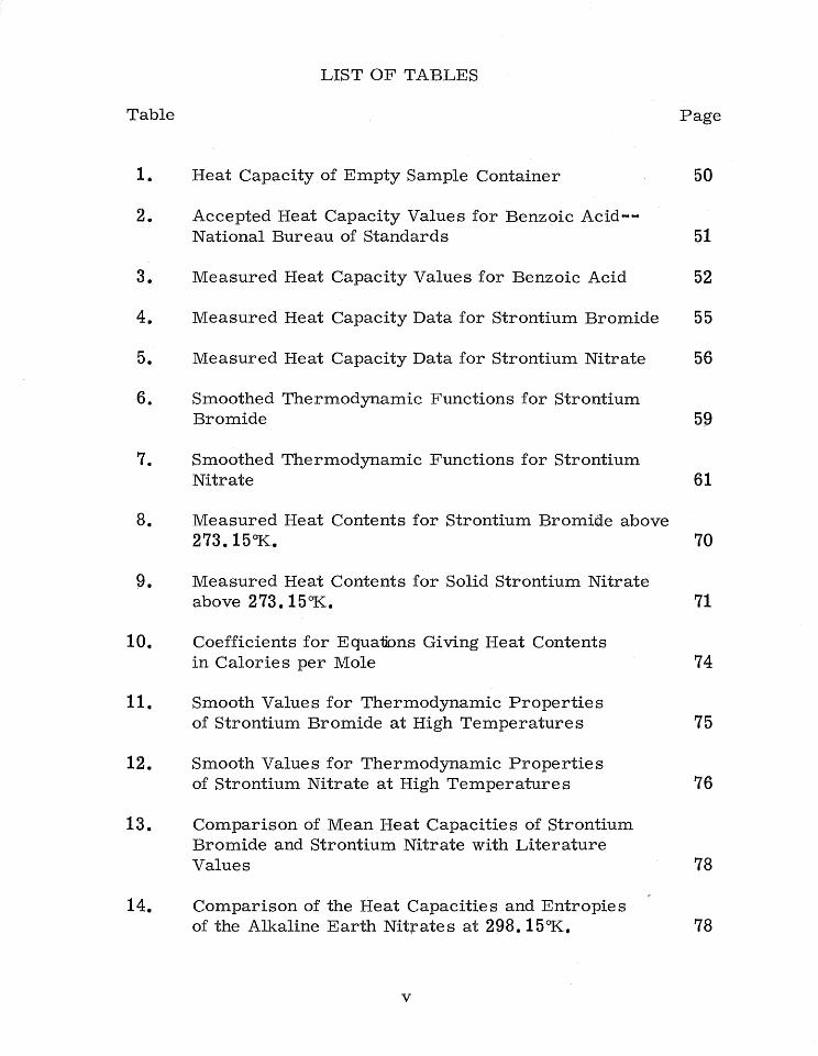
LIST OF TABLES

Table Page

1. Heat Capacity of Empty Sample Container 50

2. Accepted Heat Capacity Values for Benzoic Acid--National Bureau of Standards 51

3. Measured Heat Capacity Values for Benzoic Acid 52

4. Measured Heat Capacity Data for Strontium Bromide 55

5. Measured Heat Capacity Data for Strontium Nitrate 56

6. Smoothed Thermodynamic Functions for Strontium Bromide 59

7. Smoothed Thermodynamic Functions for Strontium Nitrate 61

8. Measured Heat Contents for Strontium Bromide above 273.15°K. 70

9. Measured Heat Contents for Solid Strontium Nitrate above 273.15°K. 71

10. Coefficients for Equaiions Giving Heat Contents in Calories per Mole 74

11. Smooth Values for Thermodynamic Properties of Strontium Bromide at High Temperatures 75

12. Smooth Values for Thermodynamic Properties of Strontium Nitrate at High Temperatures 76

13. Comparison of Mean Heat Capacities of Strontium Bromide and Strontium Nitrate with Literature Values 78

14. Comparison of the Heat Capacities and Entropies of the Alkaline Earth Nitrates at 298.15°K .• 78

V

LIST OF ILLUSTRATIONS

Figure Page

1. Sectional View of Calorimeter 28

2. Diagram of Electric Control Circuits 34

3. Diagram of Electric Measuring Circuits 36

4. Sample Data Sheet 43

5. Low-Temperature Heat Capacities of Benzoic Acid 53

6. Low-Temperature Heat Capacities of Strontium Nitrate and Strontium Bromide 57

7. High-Temperature Heat Contents of Sr(NO3 )2 &SrBr2 72

vi

Symbol

a

b

B

C

C

Cv

d

D

E

E

F

h

LIST OF SYMBOLS

Description

Coefficient in heat content equation

Coefficient in heat content equation

Coefficient of Compressibility

Coefficient in heat content equation

Heat capacity

Heat capacity at constant pressure

Heat capacity at constant volume

Coefficient in heat content equation

Indicates a Debye Function

Indicates an Einstein Function

Energy per mole

Standard electromotive force

Free energy

Free energy of a substance in a specified standard state

Standard free energy change

Free energy change of a reaction

Units

cal. mole-1

-1 -1 cal. deg. mole

atm. -i

cal. deg. - 2mole -l

cal. deg. -l

cal. deg. - 1mole -l

-1 cal. deg. mole

erg. mole-1

volts

cal. mole-1

-1 cal. mole

cal. mole-1

cal. mole-1

Free energy change in an isothermal re-action at temperature T cal. mole -l

Planck's constant erg.sec.

vii

Symbol

H

Ho 0

K

n

n

N

p

Q

R

V

a

LIST OF SYMBOLS--Continued

Description

Enthalpy {heat content)

Enthalpy of a substance at O°K. in its standard state

Heat of reaction

Boltzmann's constant

Degrees Kelvin

number of equivalents per mole re­acting in a cell

number of experimental data points

Avagadro 1s Number

Number of atoms in the simplest compositional formula

Thermal energy

Gas constant

Entropy for a substance in a specified standard state above 0°K.

Entropy change of a reaction

Temperature

Frequency of vibration

Coefficient of thermal expansion

elastic constant

viii

Units

cal. mole-1

cal. mole-1

cal. mole-1

-1 erg. deg.

OK .•

equiv. mole-1

atoms mole-1

cal.

cal. deg. - 1mole -i

cal. deg. - 1mole-1

°K .•

cycles sec. -1

gm.cm. '""2

Symbol

LIST OF SYMBOLS--Continued

Description

elastic constant

Debye 1s characteristic temperature

Einstein's characteristic temperature

ix

Units

gm. cm-2

oK.

CHAPTER I

INTRODUCTION

This dissertation concerns a branch of physical chemistry

that began in the era when chemistry was first emerging as a

recognized branch of natural philosophy. Antoine' Lavoisier,

rrthe father of chemistry,'' conducted some of the 'first calorimetric

experiments over 170 years ago when he determined the heats of

combustion of hydrogen, phosphorus, candle wax,. and olive oil

and the heat of reaction of potassium nitrate with charcoal. Al­

though experiments concerning heats of combustion and reaction

are more properly termed thermochemistry,. the related field of

chemical thermodynamics evolved simultaneously as the laws of

thermodynamics were discovered and consolidated. Despite their

age# these fields continue to interest investigators--a fact made

evident by the numerous current re search publications dealing

with problems in thermochemistry and chemical thermodynamics.

One important practical problem falling within the realm

of this particular branch of chemistry is the determination of the

feasibility of experimentally untested reactions. Thermodynamics

affords a method not only for predicting whether a reaction will

proceed or not under given conditions but also for determining the

1

2

amount of energy which can be obtained from the process or which

must be supplied in order to make the reaction proceed. Moreover.,

the ratio of products to reactants can be calculated for any given

set of experimental conditions., and, in addition., the optimum tempera­

ture and pressure for maximum yield of product can be determined.

Before thermodynamic calculations can be made for a reac­

tion., certain properties of each substance involved in the reaction

must be known. One fundamental property that must be known for

each substance is the heat capacity and its variation with temperature.

The heat capacity represents the quantity of thermal energy gained or

lost by a body per unit change in temperature and is defined mathe­

matically by the equation

(1)

in which C represents heat capacity., Q represents heat transferred.,

and T represents temperature. Heat capacity is a property propor­

tional to the quantity of matter present and is therefore classified as

an rrextensiverr property. When based on 1 gram of material., the

heat capacity is usually called n specific heat" and the dimensions~

as seen from equation (1)., may be expressed in calories per degree

per gram. A form of the heat capacity considered more u?eful by

chemists is that based on one m,ole of substance and commonly

designated by the term "molar heat capacity." The heat capacity

3

of a substance can have a definite value only under certain speci­

fied conditions., the two most importing conditions being constant

pressure and constant volume.

Because of its relationship to chemical equilibria., the

problem of accurate measurement of heat capacities has received

considerable attention in recent years and has led to important

contributions in the fields of crystal and molecular structure. Two

general methods used for determining heat capacities at different

temperatures are

(1) direct measurement (2) indirect determinations from enthalpy measurements.

For direct measurements, small measured quantities of

heat are put into the sample and the temperature rise determined

under adiabatic conditions; elaborate shielding and insulation are

necessary to prevent the exchange of heat between the sample and

its environment. "Adiabatic" calorimeters working on this principle

are presently considered the most accurate means available for

determining heat capacities below room temperature.

For indirect determinations., the enthalpy or heat content

(H) is measured at different temperatures. The rate of change in

enthalpy with temperature is numerically identical with the heat

transferred in a constant pressure process. Changes in enthalpy

can be measured readily by experimental methods and can be re­

lated to the heat capacity at constant pressure (Cp) by the equation

C =( 0 H~ p OT p

4

(2)

The investigation discussed in this dissertation was con­

cerned with four principal objectives: (1) the design and construc­

tion of a calorimeter capable of accurately measuring heat capaci­

ties from 300° K. down to 60° K. or lower temperatures., (2) the

determination of the accuracy and reliability of the calorimeter,

(3) the utilization of this calorimeter to measure the heat capacity

of strontium bromide and strontium nitrate., two compounds not

studied previously by calorimetric methods., and (4) the extension

of these heat capacity measurements on strontium bromide and

strontium nitrate to as high a temperature as practicable using

a Bunsen ice calorimeter. To meet the first of these objectives.,

a low temperature adiabatic calorimeter was constructed using a

l modification of the calorimeter described by Ruehrwein and Huffman

for the basic design. Heat capacity measurements were made on

a sample of benzoic acid obtained from the National Bureau of

Standards. The results of the measurements on benzoic acid com-

pared favorably with similar measurements by the Bureau of Stand­

ards and indicated that the accuracy and reliability of the calorimeter

1 R. A. Ruehrwein and H. H. Huffman., J. Am. Chem. Soc • .,

65., 1620., (1943).

5

built for this investigation were satisfactory. Experimental heat

capacity measurements were made with the calorimeter at tempera­

tures ranging from 60 to 300° K. on strontium bromide and strontium

nitrate. Enthalpy measurements made with a Bunsen ice calorimeter

extended from 300° to nearly 1000° K. on both strontium compounds.

CHAPTER II

THEORY

A brief discussion of the basic theory involved in chemical

therrnodynarnics will illustrate the applications of heat capacity

data and the problems involved in obtaining accurate experimental

data.

1. Free-Energy Changes in Chemical Reactions

Before a prediction of the desirability or feasibility of a

chemical process can be rnade, a knowledge of the equilibria in­

volved is necessary. The free energy change., calculable from. ex­

perimental data., is the criterion as to whether or not a chemical

reaction will occur at constant temperature and pressure.

Free energy is a single-valued., extensive therrnodynarnic

property subject to regular rnathernatical operations and is de­

fined by the equation

F = H - TS (3)

in which H represents enthalpy or heat content and S represents

entropy. For an isotherm.al process, the change in free energy

obtained from. equation (3) is

AFT = AH - TAS . (4) I

Equation (4) is important since it relates AF to the quantities AH

6

7

and .6.S which may be obtained from calorimetric measurements.

In a chemical reaction

aA + bB + ••• ----) gG + hH + ...• (5)

the free energy change at constant temperature and pressure is

given by

.6.F T p = ~F (products) ., LF (reactants) . (6)

The standard free energy change .6.FT is the change in free

energy for a chemical reaction at a specified temperature T in which

reactants in their standard states go to products in their standard

states. The standard state must be specified in every case since

0

the valte of .6.F T depends on the standard state employed. The

standard free energy change is related to the equilibrium constant

KT of a chemical reaction by the equation

(7)

Four general methods are available for determining free

energy changes accompanying reactions:

1. The equilibrium constant may be measured and equation

(7) used to calculate the free energy change. This method is not

generally applicable, however., since experimental difficulties at

high temperatures usually preclude equilibrium measurements.

2. The reaction may be allowed to take place reversibly

in a galvanic cell., in which case

~F0 = -nFE 0

T (8)

8

where n is the number of equivalents per mole reacting in the cell~

F is Faradayt s constant and E° is the standard emf of the cell. Since

relatively few reactions can be made to occur reversibly in galvanic

cells., this method is quite limited in usefulness.

3. Spectroscopic data may be used as an indirect method

to obtain free energy data. This method is applicable only to reac­

tions in which both reactants and products are gases.

4. Use may be made of the general equation sometimes re­

ferred to as a mathematical expression of the second law of thermo­

dynamics

0

~F = T

(9)

0

Here, ~HT is the heat of reaction and ~ST is the entropy of reac-

tion., both at the temperature T° K. with reactants and products in

specified standard states. This expression is usually the best and

may be the only method for determining the free energy change for

a particular reaction. In many reactions., it is a relatively simple

matter to obtain the heat of reaction., ~HTJ with the reactants and

products in their standard states. The problem is thus reduced to

finding the corresponding entropy change, ~ST, which in turn may

be accomplished by properly combining the absolute entropies of

the compounds taking part in the reaction

~S 0 = ~S 0 (products) - ~S 0 (reactants) . (10)

9

The most important method for evaluating the absolute entropies

of compounds is the use of the third law of thermodynamics in

conjunction with low temperah .. re heat capacity data.

2. Entropy and the Third Law of Thermodynamics

The entropy of any substance at a temperature T and at a

given pressure may be expressed by the equation

S = S0 + J (Cp/T) dT

0

(11)

Where S0 is the entropy at absolute zero. From equation (11) it

is evident that if the value of S0 were known, it would be possible

to derive the absolute entropy at any temperature from heat

capacity data alone.

Enlarging upon the ideas of W. Nerst's "heat theorem.,"

which now is considered mainly of historical interest, M. Plank

(1912) advanced a hypothesis concerning S0 which has become known

as the third law of thermodynamics. Unlike the first and second

laws., which advanced the concepts of energy content and entropy.,

the third law leads to no new concepts but only places a limitation

on the value of the entropy. The third law of thermodynamics stated

. 1 in its broadest form, may be written as follows:

1s. Glasstone, Textbook of Physical Chemistry, 2nd ed., D. Van Nostrand Co., Inc., Lancaster, Pa. , 1946., p. 865.

Every substances has a finite positive entropy, but at the absolute zero of temperature., the entropy rnay become zero., and does so become in the case of a per­fectly crystalline substance.

10

Thus, according to the third law., S0 rnay be taken as zero in equa­

tion (11) for perfectly crystalline substances reducing the problem.

of evaluating the entropy of such a solid to the determination of heat

capacity at a series of temperatures down to absolute zero. Equa­

tion (11) shows that if the values of C /T are plotted against T., p

or alternatively., the values of Cp against 1 n T., the area under the

resulting curve from. 0° K. to any temperature T gives the entropy

of the solid at this temperature and at the pressure at which the

heat capacities were measured.

Two important qualifications rnust be kept in rnind when using

equation (11) to evaluate entropies:

(1) The heat heat capacity rnust be a continuous function of temperature between the temperature limits.

(2) For S0 to be zero at T = 0° K • ., the substance rnust be "perfectly crystalline."

Provided a substance becomes perfectly crystalline as 0° K. is

approached., discontinuities in the variation of heat capacity with

temperature do not preclude entropy calculations since the integral

in equation (11) can be divided into temperature intervals within

which the heat capacity is continuous. Situations of this type are

quite comm.on since rnost substances undergo a transition or phase

11

change at some temperature. In addition to the heat capacity data., it

is necessary to know the heats of these transitions or phase changes

at the temperatures where they occur. As an example., consider a

substance in equilibrium crystalline condition as O{) K. is approached

but which undergoes a transition at temperature T'., melts at tem­

perature T", and boils at temperature Tift., the temperatures T'.,

T", and T" t all lying within the range 0° to T°K. The integral in

equation (11) may be separated into several constituent parts:

Tl

= s- Cp (cr:;stals I)

0

+

+ +

Tl

f cp(gas) ----dT

T

T'''

T"

.6.H' + f Cp( crystals II) T + -- --------------dT

Tltt T' T

5 Cp(hT·guid) :: + t.Httr Tttt

T"

(12)

in which .6.H11 .6.Htt., and .6.H1tt are the heats of transition, fusion and

vaporization respectively.

In order for a substance to obey the third law of thermody­

namics., it must be "perfectly crystalline. " The definition of a

perfect crystal must be made quite strict in order to exclude sub­

stances that otherwise would appear as exceptions to the third law.

It is not sufficient that a substance be chemically pure and in well

defined macrocrystalline form as absolute zero is approached but

12

the concept of internal purity must also be included before a sub­

stance may be considered as perfectly crystalline. Fortunately.,

the majority of chemical compounds in the pure solid state may

be considered as perfect crystals and the use of heat capacity

measurements in conjunction with the third law to determine

entropies is therefore widely applicable.

Situations in which the third law does not apply arise when

substances nfreezen in energy states which do not represent the

minimum energy possible for the substance and temperature in­

volved. Such substances are usually found in one of the following

ca te gorie s :

(1) solid solutions

(2) amorphous substances

(3) irregular crystals

(4) compounds with strong hydrogen bonding tendencies

(5) substances that exist as equilibrium mixtures of two distinct species

It can be shown mathematically that S0 is not zero at 0° K. for

solid solutions; hence., the third law is not applicable. Glasses are

amorphous solid substances which have retained a random., liquid-

like orientation of the molecules. It has been found experimentally

that the specific heat of glasses is abnormally high as absolute zero

I

is approached and that entropy values computed from the heat capacity

13

data are far in excess of values normally obtained for analogous

crystalline compounds.

Irregular crystals., exemplified by compounds such as CO.,

NQ, or N2 0., usually possess a molecular structure which is nearly

identical in mass or electrical configuration at either end of the

major axis. It has been found that entropies determined from heat

capacity data for such substances are less by a factor (R ln n) than

the corresponding entropies calculated statistically for the gaseous

compounds. In this factor., rrRrr is the gas constant and nnrr repre­

sents the maximum possible number of equally probable configurations

of the molecule in the crystal.

The entropy of water vapor determined from heat capacity

data is less than the value calculated by statistical means. This

discrepancy is usually attributed to random hydrogen bonding. Some

substances exist in the solid state as an equilibrium mixture of two

distinct species. Solid hydrogen., containing ortho and para forms

in a 3 to 1 ratio., is an example of such substances whose entropy at

0° K. is not zero but is equal to the entropy of mixing. This entropy

of mixing is subject to calculation; when its value is added to the

apparent value of the entropy obtained from third law calculations.,

the result is in good agreement with the statistically calculated

entropy.~

14

3. Modern Theories of the Heat Capacity of Solids

In order to determine entropies from heat capacity data., it

is necessary to know heat capacities for temperatures down to abso­

lute zero. The difficulty of obtaining temperatures much below

100° K. has fostered many attempts to extrapolate the heat capacity

versus temperature curve. Early theories of the heat capacity of

solids were totally inadequate to represent the decrease of heat

capacity with decreasing temperature. Dulong and Petit., and Kopp

proposed general values for the heat capacities of all solids., such

values being temperature independent.

In 1907., Albert Einstein2 made the fir st notable contribution

to the theory of heat capacity when he applied Planckts quantum

hypothesis to the problem of the heat capacity of solids. Einstein

considered a solid as consisting of vibrating dipoles behaving as

linear harmonic oscillators whose mean energy of vibration., e., is

given by

_ hv/kT e = hv/(e -1} (13)

where his Planckrs constant, k is the Boltzmann constant., and v

is the characteristic frequency of the oscillator. If a mole of a

monoatomic solid is considered as composed of N atoms arranged

in a cubical space lattice., each atom having 3 degrees of freedom

2

Albert Einstein., Ann. Phys. (4)., 22., 180., (1907).

15

the energy per mole is then

hv/kT E = 3Nhv/ (e ... 1) . (14)

Since the heat capacity at constant volume., C ., is defined as V

(15)

Einstein1s equation for the heat capacity at constant volume is

C ... _ (aE) hv/k1/ hv/kT = 3Nk(hv/kT/ e (e ... 1)2

V oT V

(16)

If Nk is replaced by the gas constant., R., and a constant., 9E., is

defined so that

(17)

equation. (16) simplifies to . . /

€v = 3R (9E/T)2 e 9

E/T I ( e9E1l -1)

2 (18)

which is known as Einsteints equation. According to equation (18).,

Cv should approach zero at low temperaturesi at high temperatures.,

Cv should become equal to the classical value., 3R. For most

elements., 9E/T is small at ordinary temperatures and the atomic

heat capacity is approximately equal to 3R or 6 calories per degree

per mole; however., if 0E is large., as it is for substances such as

diamond where the atoms are firmly bound., a much higher temp•

erature may be necessary before the heat capacity increases to 3R.

In equation (18)., QE is a constant for a particular substance and the

16

plot of Cv versus T gives a curve similar to the experimental

curves., the exact shape depending on the value of 9E which must

be determined experimentally.

At low temperatures, Einsteints equation (18) reduces to:

(19)

Values of CV determined at low temperatures by equation (19) fall

off more rapidly than do the experimental results.

In 1912, P. Debye3 advanced a theoretical improvement on

Einsteints treatment of heat capacities which resulted in an equation

that represented experimental results more exactly. While the

Einstein treatment postulated a lattice of independent atoms all

oscillating at the same frequency, Debye assumed that atoms vi­

brated throughout a whole spectrum of frequencies. Applying the

theory of elasticity to an isotropic elastic solid of volume, V,

Debye showed that the number of vibrations, z, below a definite

frequency,. v., was given by the equation

z = v3 VF. (20)

In equation (20}, F is a function of the elastic constants., .A and µ., 4

3 P. Debye., Ann. Phys • ., (4)., 22., 789., (1912).

4In Equation (21)., the el9-stic constants ,,l and µ are defined in such a way that Young 1s modulus., E, is

E = µ (3 ,,l. +2µ) / ( ,l + µ ) and Poissonrs ratio, 11. is

11_ =X-/2(fa+ µ)

17

and the density, t<), of the crystal and is given by the expression

(21)

When a crystal is in thermal motion., three sets of waves

will be set up in the crystal., one longitudinal and two transverse.

This means that in a mole of solid containing N atoms there will

be 3N modes of vibration., and if a maximum frequency of vibra­

tion (v ) is assumed., equation (20) becomes m

3N = v3 VF m

the differential of equation (20) is

2 dz = 3VF v dv

(22)

(23)

Eliminating the VF factor by combining equations (22) and (23)

yields

dz = 9N v2 dv

v3 m

(24)

Equation (13) states that the average energy of one mode

of vibration is

hv/kT e = hv/ (e - 1) (13)

Therefore, the total energy, E., of a solid vibrating at all frequencies

up to a maximum frequency, v ., is given by the equation m

V m 9Nh

E = 1; dz = vs m

0

18

Tre quantity hv/k has the dimensions of temperature. The

special value hvm /k, called the 11 characteristic temperature 11

(9D), has a definite value for every substance. The factor hv /kT

is dimensionless so that replacing it by the variable, x, and sub-

stituting gD for hvm/k in equation (25) yields

gD/T

J x3

_e_x __ -1---ux. (26)

0

Differentiation of equation (26) with respect to temperature gives

the Debye heat capacity equat:oni~:dx

CV = 9Nk 4(T/9) ex - 1

0 0n/T 1 e -

(27)

X In equation (27) when T is large, x becomes small, e may

be approximated by 1 + x, and the Debye equation reduces to the

classical form, Cv = 3R. Thus, both the Debye and Einstein

theories fail to explain the existence of heat capacities larger

than 3R which have been observed experimentally for the alkali

metals. As T approaches zero in equation (27), the upper

limit on the integral approaches infinity, allowing the integral

to be evaluated as 71' 4 /15; at the same time, the last term be­

comes negligible. At low temperatures then, the Debye

equation reduces to

or

3 C = aT V

where 11a" has been substituted for the constant multipliers.

19

(28)

(29)

Equation (29), usually considered valid when (Hn/T) > 10, illus­

trates one of the more significant consequences of the Debye theory

of the heat capacity of solids--the fact that the heat capacity at

constant volume is proportional to the third power of the absolute

temperature at low temperatures.

The Debye equation may be written as

(30)

which means that if CV is plotted against T / 9D the same curve

should result for all solid monoatomic elements. This has been

demonstrated experimentally for many diverse substances such as

aluminum and diamond.

The heat capacity theories of Einstein and Debye cannot be

applied directly to non-cubic or polyatomic crystals due to the

limitations imposed by their initial assumptions:

(1) isotropic crystal (cubic lattice)

(2) complete mechanical and electrical symmetry.

Born and von Karman5 modified the assumptions of Einstein and

5 Born and von Karman., Phys. Zeit . ., 14, 15., (1913).

Debye to take into account the fact that neighboring atoms in a

crystal may be non-identical. The expression resulting from

their work is

20

3 ( ~ . . 3(p .. 1) ~ SD. ~ LD __ l ·He L i=l T i=l

(31)

where D(0DJT) and E(SE/T) represent Debye and Einstein

functions respectively. Derivation of this equation was based on

the following assumptions:

(1) An atomic crystal may be regarded as composed of 11n" parallelepipeds.

(2) The heat content may be considered as being com­posed of two portions given by: a. 'Th.e sum of three Debye functions related to

elastic properties. b. The sum of 3 (p - 1) Einstein functions where

"p" refers to the number of atoms in the simplest compositional formula.

The theoretical approach of Born and von Karman furnishes the basis

for the most useful method of extrapolating heat capacity data to

absolute zero. This method is discussed in detail in the next section.

CHAPTER III

EXTRAPOLATION TECHNIQUES

Since it is impossible to obtain absolute zero tempera ..

ture and usually impracticable to obtain temperatures much be­

low 60° K. ~ some method of extrapolation is necessary to make

an accurate estimate of absolute entropies from heat capacity

data. Some of the more commonly used techniques will be dis­

cussed in this section.

1. Born and von Karman Extrapolation

Since sufficient data have not been determined in most

cases to permit evaluation of all the Debye and Einstein functions

in equation (31)., Millar1 proposed a simplified form of this equa-

tion

I (32)

i = 1

to be used to extrapolate experimental heat capacity data to abso­

lute zero. Equation (32) has been shown capable of adequately

representing heat capacity data of oxides., halides, etc., over

temperature ranges wide enough to permit accurate extrapolations.

l R. W. Millar, J. Am. Chem. Soc . ., 50, 1880 (1928).

21

22

Kelly2 has estimated a maximum error of 10 per cent in en­

tropies obtained by extrapolation from temperatures in the

neighborhood of 60° K. to absolute zero.

Carrying out extrapolations by means of equation (32) is

a trial and error process. The measured heat capacity values

are plotted against the logarithm of the temperature and the

curve extended smoothly into an estimated Debye function,

3 tables being used to obtain values of Cv as a function of 9 /T .

. D

The Debye function is drawn, extended to 300° K., and the dif-

ferences between the Debye curve and the measured heat capac­

ities at the higher temperatures are determined. These differ­

ences are plotted against the logarithm of temperature and

fitted with a series of Einstein functions. Although the results

of the first trial may not represent the heat capacity data satis­

factorily, an examination of the results will show the changes

which must be made in the Debye function to produce a better

fit of the experimental data. Usually a satisfactory fit will

be obtained after two or three trials.

The heat capacity at constant volume, C , is treated in all V

the theoretical discussions whereas the heat capacity at constant

i K. K. Kelley, U. S. Bureau of Mines Bull. 447, 1950,

p. 147.

3 Landolt- B8rnstein, Physikalische-Chemische Tabellen, J. Springer, Berlin, 1st Supp., (1927), pp. 702-'70'l.

23

pressure, Cp, is the quantity measured experimentally. Considera­

tion of the equation

C - C = a 2 VT/B p V (33)

where a and B are, respectively., the coefficients of thermal ex­

pansion and compressibility., and V is the atomic volume, shows

that Cp - Cv approaches zero as T approaches zero. It has been

found experimentally that for most substances the difference be­

tween Cp and Cy at temperatures below 60° K. is less than preci­

sion of measurement and therefore negligible.

Nernst and Lindermann4 have proposed that Cp - Cy may

be evaluated for numerous solids from the equation

Cp - Cv = o. 0214 Cp (T /Tm) (34)

where Tm represents the melting point in degrees Kelvin. Since

the magnitude of the difference Cp - Cy is small, equation (34)

can be applied to Cp data at low temperature in order to fit experi­

mental data with Debye and Einstein functions without introducing

appreciable error.

2. Debye Extrapolations

For monoatomic elements crystallizing in a cubic lattice.,

equation (27) has been found usually to represent experimental

data within the limits of accuracy of these data. The value 8D

4Nernst and Lindermann., Zeit. fur Electrochem • ., 17, p. 817, (1911).

24

must be determined, however, before equation (27) can be used to

represent heat capacity data. Debye showed that 8D should be re­

lated to the elastic constants, A and µ, of the medium, which

were discussed on page 16.

As an approximation, it may be assumed that the Debye and

Einstein frequencies are the same. In this case Einstein5 has shown

that the characteristic frequency of a substance may be calculated

from the specific volume, compressibility, and molecular weight.

Rubens6 and collaborators utilized the phenomenon of se-

lective reflection for determining the characteristic frequencies of

substances. When polychromatic light is incident upon a solid, the

reflected rays are deficient in certain wave length regions. These

regions of 11residual rays" indicate the characteristic frequencies

of the solid required for use in the heat capacity equations of Einstein

and Debye.

Since sufficient data are seldom available, it is usually neces­

sary to obtain 9n by determining the heat capacity at a known temper­

ature experimentally. In the few cases where sufficient data are

available, the calculated values of characteristic temperatures

agree closely with experimental heat capacity results.

5 A. Einstein, op. cit. , p. 180.

6 ' Rubens and Nolnogel, Phil. Mag. 19, 761, (1910).

25

3. Empirical Relations

Lewis and Gibson7 have utilized the general expression

(n < 1) (35)

where fD represents the Debye function, to successfully represent

the heat capacities of a number of compounds. By choosing appro­

priate values of 11n 11 the relationship has been found to hold for

iodine, sulfur, and a number of metal halides.

Nernst8 expressed heat capacity as the weighted sum of an

Einstein function (fE) and a Debye function (fD):

Cv = afE (T /{\) + bfD (T /82) (36)

where 81 and 82 are constants for a given compound. Other combi­

nations of Debye and Einstein functions have been used to represent

heat capacity data, but although many combinations represent dis­

crete portions of the data, most fail to adequately represent a major

portion of the experimental measurements. Thus entropies based

upon such extrapolations would have a large uncertainty. The Born

and von Karman approach, as modified by Millar, has a stronger

theoretical foundation and is usally more successful than empirical

relations. For this reason, the method of Born and von Karman

was selected for use in this dissertation to extrapolate heat capac­

ity data to zero degrees Kelvin.

7 Lewis and Gibson., Jour. Am. Chem. Soc. 39, 2554, (1917).

8 Nernst., Sitzb. Konig, Preuss. Akad. Wiss., p. 353., 1914.

CHAPTER IV

APPARATUS

Two types of calorimeters were used in this investigation:

(1) Bunsen ice calorimeter for high temperature enthalpy measure­

ments, and (2) adiabatic calorimeter for low temperature heat

capacity measurements. The Bunsen ice calorimeter was con-

structed in this laboratory as part of a previous investigation; an

adequate description of the construction and operation of this

calorimeter is available in previous reports. 1 ' 2 A major part

of the present investigation was to design and construct a low

temperature adiabatic calorimeter. A detailed description of

this apparatus is presented in this section.

1. Calorimeter Assembly

The calorimeter assembly consists of four principal parts:

(1) the sample container, (2) the thermal shields# (3) the outer

jacket and associated radiation shields# and (4) the vacuum system.

1 C. E. Kaylor# "Heat Capacities at High Temperatures, n a

dissertation, University of Alabama# 1958. 2 G. E. Walden, 11 The NaF - RbF System at High Tempera-

tures., 11 a dissertation., University of Alabama., 1959.

26

27

Figure 1 presents a schematic diagram of the calorimeter used in

this re search.

The sample container., L., a cylindrical copper container,

1 1/2 inches in diameter and 3 inches long., has hemispherical

ends. The container., made of O. 01-inch copper foil., has a ther•

mometer well., M., (3 / 8 by 2 inches) surrounded by 6 copper vanes

which facilitate transfer of heat to the sample. The sample heater

and platinum resistance thermometer are arranged concentrically

inside the well. The sample heater consists of about 13 feet of

No. 34 B. W. G. nickel-chrome enameled wire (230 ohms total

resistance) wound bifilarly on a stainless steel tube. The winding

was wrapped with lens paper., impregnated with insulating varnish.,

and baked at 110° C. for several hours. The finished heater fits

snugly into the thermometer well and the thermometer fits snugly

inside the heater. Apiezon M grease was applied to both ther ...

mometer and heater before their insertion into the well to increase

thermal conductivity. Once the heater and thermometer were in•

serted into the well, they were not removed until all measurements

had been completed. This assured that no change would occur in

the heat capacity of the container due to different weights of grease.,

etc.

A small screw was sold~red to one side of the sample con ..

tainer so that one junction of a copper•constantan difference

28

A Q

p B

C 11 II I ,, 11 II I

,, 1111 I ,: 1111 l

,, j I II I

,, D 1.111;

,, ,, 0

ii ii I II i 1 [I I 1' I I II I 11 if f I f I II I I 1111 I II II I

A. Windlass 11 !I l I I II I

B. Neoprene "O" ring I I II I

: : H : C. Brass case 11 II I D. Metal Dewar vessel , , 11 I

11 :: I E. Upper tanK F. Radiation shield

F G. Economizer H. Lower tank

G i. Radiation shield J. Outer adiabatic shield K. Inner adiabatic shield L. Sample container

ii M. Thermometer well ii Ii N. Ring ii 0. Outlet to vacuum ,,

H 11 P. Nylon string II II Q. Lead-wire outlet II ii II 11 II 11 II

29

thermocouple could be attached. This thermocouple indicates the

magnitude and direction of the temperature difference between the

sample container and the adiabatic shield. A short length of 1 / 4 -

inch m.onel tubing inserted in the upper end of the container pro­

vided an opening for loading. This m.onel metal tube was pro­

vided with a copper cap which could be soldered in place to pro­

vide a vacuum. tight seal. The outside of the sample container

was gold plated to m.inim.iz e oxidation and to decrease the in -

evitable radiation losses. The empty container had a weight of

about 63 g • ., an inside volume of 70 m.l. 1 and a heat capacity of

approximately 6. 5 cal. /degree at room. temperature.

Surrounding the sample container are two gold plated

adiabatic shields, J and K., one inside the other. The cylindrical

shields are constructed of O. 015-inch sheet copper and have hemi­

spherical ends. The inside shield., K, is 2 1 /2 inches in diameter

and 5 inches long., while the outer shield., J, is 3 1 /2 inches in

diameter and 6 inches long. The outer surface of each shield was

covered with three separate bifilar windings of No. 36 B. and S.

gauge teflon covered copper wire. Difference thermocouples

were attached between the top., bottom.., and side of each shield

and between the sides of the inside and outside shields. These

difference thermocouples enabled detection of any differences in

temperature along the surface of the shields. This difference could

be corrected by adjusting the current in the appropriate heater

winding. All electrical wires leading to the adiabatic shields.,

30

the thermometer, and heater were wound around a ring, N., whose

temperature was kept within a few degrees of the temperature of

the outside adiabatic shield by using an auxiliary heater and dif­

ference thermocouple.

The sample container, adiabatic shields, and ring are

surrounded by a copper radiation shield., I., which is attached to

the lower tank, H., by a threaded connection. Apiezon M grease

was used on the threaded connection to insure good thermal con­

tact between the radiation shield and the lower tank. In a similar

manner another radiation shield, F, was attached to the upper

tank., E., and surrounded the lower tank and its attached radiation

shield. A stainless steel dewar flask., D., 7 1/2 inches inside

diameter and 36 inches high, contained the upper and lower tanks

and their attached shields and minimized heat transfer into the

system. The whole assembly was enclosed by a vacuum tight

brass case, C., which was attached to a top plate with thumb screws,

a neoprene "Orr ring, B, effecting a vacuum tight seal.

The upper tank was supported from the top plate by two

3 /8-inch stainless steel tubes. One of the tubes extended into the

tank and ended about 3 / 4 inch from the tank bottom, while the other

tube barely entered the top of the tank. The longer tube was used

31

to fill the tank with liquid air. When it was desirable to remove

liquid air from the tank, compressed air was blown into the shorter

tube and the liquid air was ejected through the fill tube. The lower

tank was supported from the top plate by two 3 /8-inch stainless

steel tubes connected in the same fashion as the top tank. These

tubes passed through the upper tank, but were not fastened to it.

A 1 / 4-inch copper tube., G., also entered the lower tank and was

coiled several times between the upper and lower tanks. This tube

was called an economizer since gases coming from the evaporating

liquid in the lower tank were forced to pass through the coiled tube

and absorb additional sensible heat. A vacuum pump was attached

to the economizer outlet when temperatures lower than that of

liquid air (86°K. ) were desired.

Figure 1 shows the calorimeter in operating condition with

the sample container supported by a nylon string extending from

the windlass., A, to the top of the container. The outer adiabatic

shield is supported by three nylon strings attached to the ring while

the inner adiabatic shield is supported by three nylon strings at­

tached to the outer shield. Conical copper fittings were attached

to the sample container, both adiabatic shields., and the bottom of

the lower tank to increase the contact area and thus decrease

thermal resistance to conduction when cooling the sample to low

temperatures.

32

The brass case, C, was connected to a vacuum system

through the tube., O. An oil diffusion pump., backed by a mechani­

cal pump., was operated continuously to supply the vacuum while

measurements were in progress. The ultimate vacuum attained,

as indicated by an ionization gauge, was 9 x 10""5 mm. of mercury.

2. Electric Control Circuits

Keeping the temperature difference between the adiabatic

shield and the sample at a minimum is of primary importance in

the operation of an adiabatic calorimeter. The temperature dif­

ferential between sample and shield and between the top., bottom.,

and side of each adiabatic shield was measured by means of copper­

constantan difference thermocouples described in the preceding

section. These seven difference thermocouples were divided into

two groups: (1) the difference couples between the inner shield

side and sample, the inner shield side and top, and the inner shield

side and bottom., (2) the difference couples between inner and

outer shields, outer shield side and top, outer shield side and bot­

tom., and outer shield side and ring. The two groups of difference

couple leads were connected through separate rotary selector

switches to two galvanometers. Rotation of the appropriate se­

lector switch allowed simultaneous observation of temperature

differentials in the inner and outer shield areas. The two

33

galvanometers had a sensitivity of O. 5 microvolts per millimeter

at one meter distance and were used in conjunction with a scale

located two meters from the galvanometers., thus doubling their

sensitivity.

The temperature differences observed by means of the dif­

ferential couples and galvanometers were controlled by varying

the current in the resistance heaters described in the preceding

section. Figure 2 shows the control system used to regulate the

current flow in the shield heaters. The resistances marked side,.

bottom., top., ring., etc. represent the heaters on the respective

parts of the adiabatic shield system. A transformer reduced the

110-volt line voltage to 24 volts for use in the shield heater cir­

cuits. As Figure 2 shows., a special 3 position switch was pro­

vided in each heater circuit so that two resistors could be shorted,

providing a quick increase in heater current. These heater surge

switches were normally off in the middle position but could be

closed temporarily by holding in the down position or closed for

longer periods without holding by placing in the up position. For

more sensitive current regulation., a power stat was placed in each

heater circuit.

- II 24-volt

60 ""a.c

Heat-surge switch

Meter range

Powerstat Powerstat Powerstat

Top Side Bottom

INSIDE SHIELD

Powerstat Powerstat Powerstat

Top Side Bottom

OUTSIDE SHIELD

Fig. 2. Diagram of Electric Control Circuits

Powerstat

ma.

120 n.

Ring

~ 31'5

c...., >+:>-

35

3. Electric Measuring Circuits

Operation of an adiabatic calorimeter requires an accurate

measurement of three quantities: (1) initial temperature., (2)

heat input., and (3) final temperature. To determine the heat

input., measurements must made of current., voltage., and heating

time. Figure 3 shows the electric circuits used to make the

necessary measurements. The temperature measurements were

made with a Mueller resistance bridge by determining the re­

sistance of a four-lead capsule type platinum resistance ther­

mometer. Both the bridge and the thermometer were calibrated

by the National Bureau of Standards; the resistance thermometer

had an approximate resistance of 25 ohms at 0° C. A table of

temperature-resistance values was supplied with the thermometer

calibration by the Bureau of Standards. While the Mueller bridge

could be read directly to the nearest O. 0001 ohm by correctly

adjusting the resistance decades., it was easier to determine the

last significant figure of the resistance reading by utilizing a tele­

scope to read the deflection of the bridge galvanometer on an il­

luminated scale reflected in the galvanometer mirror. The il­

luminated scale and the bridge galvanometer were placed 6 meters

apart to increase the accuracy of the readings.

The circuits used for measuring the energy supplied to the

sample heater are shown in Figure 3. The d. c. voltage necessary

Potentiometer

2-16-volt d.c.

Volt box

Potentiometer

1-ohm standard resistor

Double pole, double throw switch

• (1 I Timer I 110-volt 60 .,, a.c. _ • I j

Heater

Dummy heater

Fig. 3. Diagram of Electric l'vTeasuring 1----:ircuits

Mueller bridge

~ 113,f.

37

for heating was supplied by Willard 2--:rolt lead storage cells con­

nected in parallel banks of four cells each. The supply voltage

could be varied in 2-volt increments from 2 to 16 volts. In order

to measure the voltage drop across the sample heater I it was

necessary to reduce this voltage to a value that could be read on a

potentiometer (O - 1. 6 volts). This was accomplished by using

a volt box or potential divider which provided a reduction ratio

of 10 to 1. The current through the heater was determined by

measuring the potential drop across a standard one-ohm resistor

connected in series with the heater, subsequently making a cor•

rection for the current flowing in the volt box circuit. Two Leeds

and Northrup K-3 potentiometers were used for the current and

voltage measurements. When the current was not flowing through

the sample heater I it flowed through a dummy of equal resistance

so that the battery current was constant.

The heating time was measured with a synchronous timer

which was started and stopped at the same time as the heater cur­

rent by using a double pole switch. The time of heating could be

read directly from the timer to 0.1 second and estimated to the

nearest 0. 01 second.

CHAPTER V

OPERATION

1. Loading the Sample Container

The sample container was weighed empty, then loaded with

dry sample through the 1/4-inch monel tube and reweighed. Next

the copper filler cap was soldered in place with woods metal,

closing the container except for a small pin hole in the center of

the cap. After thoroughly evacuating the container, helium gas

was admitted and the pin hole sealed with a pressure of 1 atmos­

phere of helim inside the container. The helium gas provided a

highly conductive medium for heat transfer within the calorimeter

thus decreasing the time required for the establishment of equilib­

rium after a heating period. Monel metal was selected for the

filler tube because it is a poor conductor of heat and would there­

fore minimize the transfer of heat to the sample container while

the filler cap was being soldered in place.

After the sample container had been filled with helium and

sealed, it was suspended from a nylon string attached to the windlass.

Finally, the sample container difference thermocouple was attached

and the thermometer and heater lead wires connected by soldering.

38

39

After closing the adiabatic shields, attaching the radiation shields,

and securing the outer brass case to the top plate, the mechanical

vacuum pump was started. The system was evacuated for several

hours with the mechanical pump before the oil diffusion pump was

started. The latter was allowed to operate for at least 12 hours

before heat capacity measurement were begun, this amount of

time being necessary to reach a pressure of 9 x 10-5 mm. of

mercury.

2. Measurement Procedure

After the calorimeter had been assembled and evacuated,

the windlass was used to raise the sample container and adiabatic

shields into contact with the bottom of the lower tank. Liquid air

was introduced into the upper and lower tanks, cooling the sample

to a temperature of about 86° K. in 16 hours. An additional 12 hours,

was required to cool the apparatus to 60° K.; this was accomplished

by reducing the pressure on the liquid air in the lower tank.

After the sample had cooled to the de sired temperature,

the sample container and adiabatic shields were lowered into

operating position and measurements begun. Two operators were

required to operate the calorimeter control and measurement

systems. The energy input and temperature measurements were

controlled by one operator while the adiabatic shields and ring

40

were controlled by the second operator. After the sample tempera­

ture had been observed for a short time the heating period was

begun. The double pole switch was closed to start the heater cur­

rent and the timer simultaneously. Voltage and current measure­

ments were made after 21 per cent and 79 per cent of the time

interval of heat input had elapsed. The average current and voltage

was assumed to be the mean of the currents and voltages recorded

in accordance with the work of Gibson and Giauque. 1 Prior to open­

ing the switch at the end of the heating period., the shield operator was

notified and, at the proper moment, the double pole switch was opened.

Four or five minutes were allowed to pass for thermal equilibrium

to be restored in the sample container; then temperature readings

were taken and recorded at one .. minute intervals until a uniform

temperature drift was established. After the temperature drift

rate had been determined, another heating period was started. A

heating current was selected to produce a temperature rise of ap­

proximately 5 degrees in a 5-minute heating period.

l G~ E. 0-ibson. and W. F. Giauque, J. Am. Chem. Soc.,

45., (1923), p. 99. These workers showed that the current passing through the heater varied with the time beaause (1) the resistance increased as the temperature of the heater increased and (2) the batteries discharged slowly during use. The overall variation of current with time was found to be consistent with a quadratic equa­tion of the type I =A+ Bt + Ct2 ., By integration of this equation be­tween limits., Gibson and Giauque showed that the averages of the 21 and 79 per cent readings represented the average emf and amper­age values satisfactorily.

41

The adiabatic shield operator was responsible for minimizing

heat transfer by radiation to the sample container. By observing

the deflection of two illuminated hairlines on a frosted glass scale.,

the shield operator was able to observe temperature differences

detected by the difference thermocouples described in the section

entitled rrApparatus rr. The inside shield temperature was kept as

close to the sample container temperature as possible at all times.

Galvanometer sensitivity enabled the detection of 0. 25 microvolts

as a hairline deflection of 1 millimeter on the glass scale. Since

a copper-constantan thermocouple generated about 15 microvolts

per degree at 60°K . ., one-millimeter deflection corresponded to a

temperature difference of about O. 02°C. At 300°K. a copper­

constantan couple generates 41 microvolts per degree, correspond­

ing to a temperature difference of only 0. 006°C. The difference

between the inner shield temperature and the sample temperature

was kept smaller than a value corresponding to a galvanometer

deflection of about 2 millimeters from the balance point except at

the beginning and end of a heating period when deflections of 5 or 6

millimeters might exist temporarily.

The outside shield served to isolate the inside shield from

cold surroundings., enabling the temperature of the inside shield

to be controlled closely and easily with only small currents flowing

in the inner shield heaters. The outer shield was kept a few tenths

of a degree cooler than the inside shield to provide a small cooling

42

effect. The ring temperature was not particularly critical since

two adiabatic shields were used., and the ring temperature was

roughly controlled to within a few degrees of the outer shield

temperature.

3. Recording and Calculating Heat Capacity Measurements

Figure 4 is a sample of the data sheet used when recording

the measurements made in this investigation. Before the heating

period was started the Mueller bridge was balanced to a scale

reading of a few centimeters from. the gal vanom.eter zero posi ....

tion. The bridge reading (BR), scale reading (S ), and galvano-c

meter zero (G0 ) were recorded on the data sheet immediately

before the heating period was started. Next, the switch was

thrown starting the heating period. The time of day was re -

corded when the heating period began, and voltage (E) and

current (I) were recorded in the appropriate spaces after 21 per

cent and 79 per cent of the total heating time had passed. After

the selected time had elapsed (usually 5 or 6 minutes) the heat-

ing current was turned off, the time of day was again recorded,

and the heating time was recorded from. the synchronous timer

to the nearest 0. 01 second. After waiting 5 or 6 minutes for

therm.al equilibrium. to be established, the Mueller bridge was

balanced again and a temperature ' 1driftn was observed until a

constant rate was reached. The drift was determined by recording

43 Compound: Benzoic Acid Operators: Taylor and Smith

Date: Dec. 26, 1960. Time Heat on: 11 :42 Calculated by: __I_

Checked G G0 47 cm

50 cm E(volts) I(amps)

13,959 .05857 -3 cm

13,941 • 05847 ~ x • 000134 = - • 000402 ohms

avg. 13,950 • 05852 BR 12. 8990 ohms

E/3000 • 00465 Time cBR 12. 898598 ohms

13. 950 x • 05387 x 359. 93 x • 239006 = 64. 64695 cal.

Time Heat Off 11 :49

(driftx time) + (G0 - S ) C

( 0 X 12) + {1_Q -_1a) X • 000134 = ~ 000402

FBR 13. 4510 FcBR 13. 450598

T = 156. 690 2

T1 = 151. 512 ~T= 5.178 Tm = 154.10° K dH/dT = 12. 485 ------

Figure 4. Sample Data Sheet

Drift Sc(cm) Time

11 :58 50 :59 49 :60 49 :61 49

44

time and scale readings at one-minute intervals.

The data sheet is arranged so that the scale reading, Sc,

in the upper right corner is always subtracted from the gal vano­

meter zero, G0 ., just above it. The difference, ~, which may be

positive or negative, is multiplied by a predetermined constant

converting~ into an equivalent number of ohms. The product of

~ and its conversion factor is added algebraically to the Mueller

bridge reading., BR, giving the corrected bridge reading., cBR.

The value cBR is the reading the Mueller bridge would have given

directly if the bridge had been balanced to give a galvanometer

deflection of zero. From tables furnished with the platinum re­

sistance thermometer., cBR is converted directly to the tempera­

ture., Ti, and placed in the lower left corner of the data sheet.

Average values of current and voltage are computed and

placed in the indicated lines in the upper left of the data sheet.

Since a shunt circuit was used in measuring the applied voltage.,

the current flowing in the shunt circuit., illustrated in Figure 2,

must be subtracted from the average total current. The current

in the shunt circuit is calculated by dividing the average voltage

by the total resistance of the shunt, 3000 ohms. Multiplying the

factors., average voltage, corrected average current., heating

time, and the conversion factor 0. 239006 gives the heat input in

calories.

45

The final bridge reading., FBR., is corrected for tempera­

ture drift in addition to scale correction. After uniform drift was

established., it was assumed to be constant from the end of the

heating period until the last scale reading was taken. After adding

the drift and scale correction to FBR to obtain the final corrected

bridge reading., FcBR., the same tables were consulted to obtain

the final temperature., T2 • Subtracting T1 from T2 gave -6. T., the

temperature rise during a heating period. Averaging T1 and T2

gives Tm" the mean temperature of the run. The mean specific

heat of the container plus sample., dH/dT., is the heat input divided

by the temperature rise.

In most of the experimental runs., the temperature drift was

zero or less than one centimeter per minute (0. 0001 degree per

minute). The constant used for converting the scale reading to ohms

depended on the galvanometer sensitivity and the scale and telescope

positions. This constant changed very little with time., but was

carefully determined before beginning each set of measurements.

CHAPTER VI

COMPOUNDS AND THEIR PREPARATION

1. Strontium Nitrate

Baker and Adamson reagent grade strontium nitrate was

used in this investigation. The label on the bottle indicated the

following impurities:

insoluble in water ci-so4 Fe Heavy metals (as Pb) Mg and alkalies

0. 01 per cent . 002

.. 005 . 0005 . 0005 .15

Spectrographic analysis confirmed the bottle label with the ex­

ception of calcium which was found present to the extent of O. 01

to O. 1 per cent. No further attempt was made to purify the

strontium nitrate; it was loaded into the sample container after

drying at 200° C. for four hours. Strontium nitrate forms no

hydrates and is neither deliquescent nor hygroscopic.

2. Strontium Bromide

The best grade of strontium bromide available for use in

this investigation was Mallinckrodt Chemical Works' chem­

ically pure strontium bromide hexahydrate. Spectrographic

46

analysis showed the following approximate concentrations of

impurities:

calcium magnesium copper tin sodium

0. 01 to 0. 1 per cent . 001 to O. 01 . 001 to . 01 .001 to .01 . 001 to . 01

Analysis for chloride ions utilizing ion exchange resins showed

that the chloride ion concentration was below 8.1 per cent. No

attempt was made to purify the strontium bromide.

Strontium bromide forms several hydrates and is quite

hygroscopic in the anhydrous form. Obtaining the anhydrous

47

salt from the hexahydrate proved.more difficult than was antici­

pated. Literature references1 ' 2 indicated that strontium bromide

could be fused (melting point 643° C.) to free the salt from com-

bined water. Fusing the strontium bromide in air, however, was

found to convert from 1 to 3 per cent of the salt to strontium

oxide. This decomposition occurred even when strontium bro­

mide was mixed with ammonium bromide before melting.

After experimentation with several small samples, it

was found that the strontium bromide hexahydrate could be

.l G. F. Huttig and C. Slonim, z. anorg. angem. Chem.,

181, pp. 65 - 77 (1929). 2 J. W. Mellor, A Comprehensive Treatise on Inorganic

and Theoretical Chemistry, Longmans, Green, and Co., Vol. III, p. 729, (1946).

48

dried without appreciable decomposition by heating at a temperature

of 400 to 450° C. for four hours. Although the salt discolored some­

what while drying at this temperature, analysis showed that con­

version to the oxide was less than 0. 1 per cent.

CHAPTER VII

LOW TEMPERATURE RESULTS

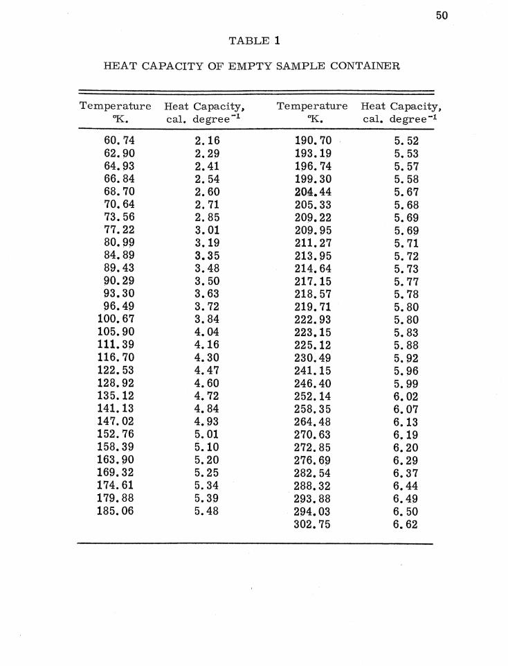
1. Heat Capacity of Empty Sample Container

Before the heat capacity of a sample could be determined

over a range of temperatures., it was first necessary to measure

the heat capacity of the empty sample container over the same

temperature range. The heat capacity measurements on the empty

container were plotted against temperature and a smooth curve

drawn through the points. The sample container was then filled

with the compound to be studied and the heat capacities of the com­

pound and container were determined over the de sired temperature

range. The heat capacity of the sample at each temperature was

determined by subtracting the empty container's heat capacity.,

which was read from the smooth curve at the corresponding

temperature. Table 1 lists the measured heat capacities of the

empty sample container.

2. Heat Capacity of Benzoic Acid

To test the reliability and accuracy of the low tempera­

ture calorimeter., heat capacity measurements were made on

benzoic acid. Benzoic acid is one of three materials available

49

50

TABLE 1

HEAT CAPACITY OF EMPTY SAMPLE CONTAINER

Temperature Heat Capacity, Temperature Heat Capacity, OK .• cal. degree-I aK. cal. degree-I

60.74 2.16 190.70 5. 52 62.90 2.29 193.19 5. 53 64.93 2.41 196.74 5.57 66.84 2.54 199.30 5.58 68.70 2.60 204.44 5.67 70.64 2.71 205.33 5.68 73.56 2.85 209.22 5.69 77.22 3.01 209.95 5.69 80.99 3.19 211. 27 5.71 84.89 3.35 213.95 5.72 89.43 3.48 214.64 5.73 90.29 3.50 217.15 5.77 93.30 3.63 218.57 5.78 96.49 3.72 219.71 5.80

100.67 3.84 222.93 5.80 105.90 4.04 223.15 5.83 111. 39 4.16 225.12 5.88 116.70 4.30 230.49 5.92 122.53 4.47 241.15 5.96 128.92 4.60 246.40 5.99 135.12 4.72 252.14 6.02 141.13 4.84 258.35 6.07 147.02 4.93 264.48 6.13 152.76 5.01 270.63 6.19 158.39 5.10 272.85 6.20 163.90 5.20 276.69 6.29 169.32 5.25 282.54 6.37 174.61 5.34 288.32 6.44 179.88 5.39 293.88 6.49 185.06 5.48 294.03 6.50

302.75 6.62

51

from the National Bureau of Standards for use as a standard in

testing and calibrating various types of calorimeters. The purity

of the benzoic acid samples has been determined as 99. 997 mole

per cent and the calorimetric properties of any two samples

should be the same within the accuracy of present experimental

apparatus. Table 2 lists smooth heat capacity values determined

by the Bureau of Standards for one of their benzoic acid samples. 1

TABLE 2

ACCEPTED HEAT CAPACITY VALUES FOR BENZOIC ACID--NATIONAL BUREAU OF STANDARDS

Temperature Heat Capacity (Cp).. °K. cal. degree -i mole-1

0 5

10 15 20 25 30 35 40 45 50 55

0 . 06 . 46

1. 46 2.63 3.95 5.24 6.47 7.57 8.55 9.44

10.23

Temperature Heat Capacity (cpt "'K. cal. degree-1 mole -i

60 80

100 120 140 160 180 200 220 240 260 280 300

10.97 13.35 15.28 17.10 18.90 20.74 22.63 24.59 26.62 28.73 30.88 33.08 35.29

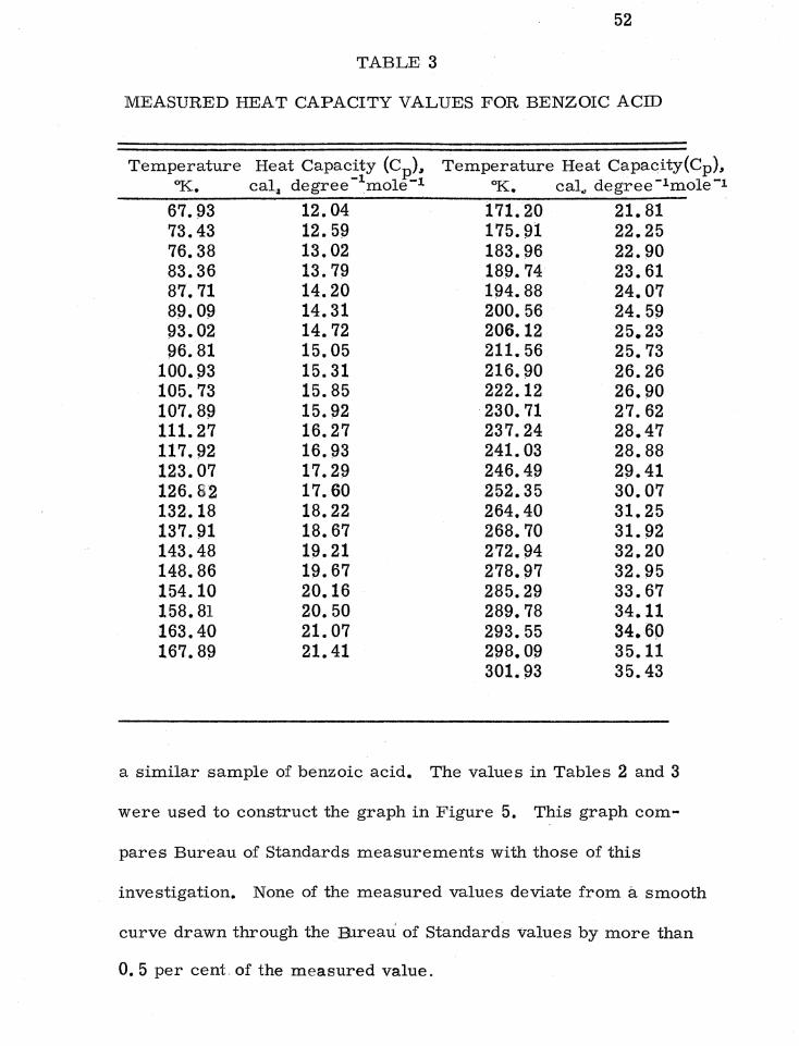
Table 3 lists heat capacities measured in this investigation on

1 G. T. Furukawa, R. E. Mccoskey, and G. J. King, l•

Res. NBS, 47 (1951), p. 256. ,

52

TABLE 3

MEASURED HEAT CAPACITY VALUES FOR BENZOIC ACID

Temperature Heat Capacity (Cp), °K. cal1 degree - 1mole-1

Temperature Heat Capacity(Cp), °K. cal., degree - 1 mole-1

67.93 12.04 171.20 21.81 73.43 12.59 175.91 22.25 76.38 13.02 183.96 22.90 83.36 13.79 189.74 23.61 87.71 14.20 194.88 24.07 89.09 14.31 200.56 24.59 93.02 14.72 206.12 25.23 96.81 15.05 211.56 25.73

100.93 15.31 216.90 26.26 105.73 15.85 222.12 26.90 107.89 15.92 230.71 27.62 111.27 16.27 237.24 28.47 117.92 16.93 241.03 28.88 123.07 17.29 246.49 29.41 126.62 17.60 252.35 30.07 132.18 18.22 264.40 31.25 137.91 18.67 268.70 31.92 143.48 19.21 272.94 32.20 148.86 19.67 278.97 32.95 154.10 20.16 285.29 33.67 158.81 20.50 289.78 34.11 163.40 21.07 293.55 34.60 167.89 21.41 298.09 35.11

301.93 35.43

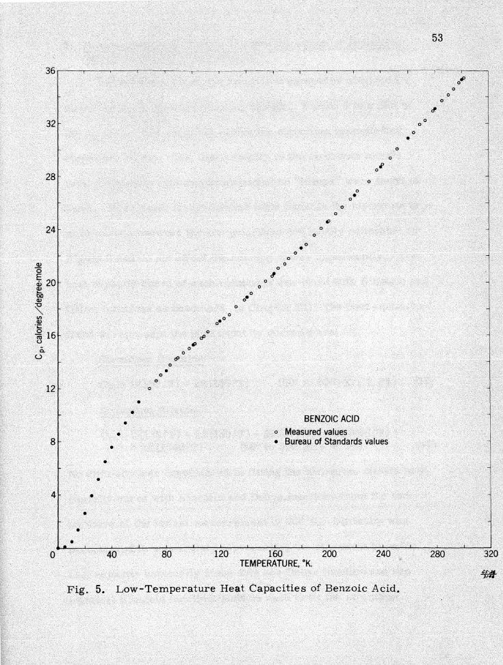
a similar sample of benzoic acid. The values in Tables 2 and 3

were used to construct the graph in Figure 5. This graph com­

pares Bureau of Standards measurements with those of this

investigation. None of the measured values deviate from a smooth

curve drawn through the B..1reau of Standards values by more than

O. 5 per cent of the measured value.

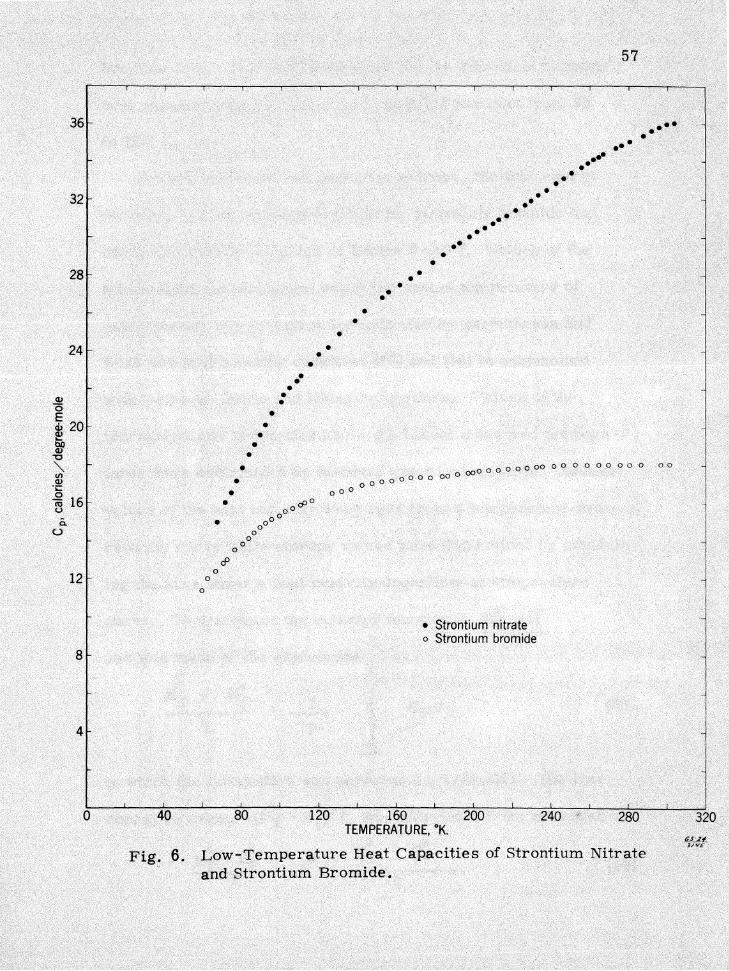
3. Heat capacity and Thermodynamic Functions of Strontium Bromide and Strontium Nitrate

Tables 4 and 5 list measured heat capacities obtained for

strontium bromide and strontium nitrate. Figure 6 is a plot of

54

the measured heat capacity values for strontium bromide and

strontium nitrate. The heat capacity of the strontium nitrate

varies smoothly with temperature and no nhumpsn were found to

exist. Some small irregularities were found in the strontium bro­

mide curve. however the irregularities are hardly noticeable in

Figure 6 and do not affect the entropy values significantly. The

heat capacity curve of each compound was fitted with Einstein and

Debye functions as described in Chapter III. The best equations

found to represent the heat capacity curves were:

Strontium Bromide

Cp = D(l50/T) + 2E(l57/T) (60° to 100° K.; 1. 8%) (37)

Strontium Nitrate

Cp = D(l33/T) + 2E(l88/T) + 2E(277 /T) + 2E(868/T) + + 2E(l 740/T) (68° to 300° K.; 0. 8%). (38)

No difficulty was encountered in fitting the strontium nitrate heat

capacity curve with Einstein and De bye functions from the tern -

perature of the lowest measurement to 300°K. Difficulty was

encountered in accourately representing the strontium bromide

heat capacity especially since only one Debye function and two

identical Einstein functioll'lB could be used to fit the strontium

55

TABLE 4

MEASURED HEAT CAPACITY DATA FOR STRONTIUM BROMIDE

Temperature Heat Capacity (Cp), Temperature Heat Capacity(Cp), °K. cal. degree - 1mole -i °K. cal. degree -1mo1e-1

60.30 63.60 67.55 70.73 73.26 77.57 80.92 84.15 87.25 90.28 93.28 96.21 99.52

103.18 106. 74 . 110.56 112.93 lit"l,.,.82 ua,r;.is 132.29 137.73 143.05 148.24 153.38 158.44 163.43

11.41 11. 97 12.38 12.78 13.04 13.54 13.84 14.14 14.41 14. 73 14.89 15.11 15.34 15. 57. 15.68 15.85 16.00 16.15 16.42 16.58 16.73 16.89 17.01 17.07 17.15 17.23

168.37 173.28 178.47 183.91 187.18 192.48 197.75 199.91 202.96 208.13 213.25 218.34 223.38 228.38 233.34 236.36 242.12 247.83 253.50 259.12 264.70 270.22 275.70 281.12 286.48 297.07 301.86

17.29 17.33 17.33 17.40 17.42 17.53 17.58 17.60 17.65 17.70 17.73 17.77 17.80 17.84 17.88 17.90 17.92 18.00 18.00 18.00 18.00 18.00 17.98 17.99 18.01 18.01 18.02

56

TABLE 5

MEASURED HEAT CAPACITY DATA FOR STRONTIUM NITRATE

Temperature, Heat Capacity(Cp)., Temperature., Heat Capacity(Cp)., oK. cal. degree-1mole-t OK .• cal. degree - 1mole-1

67.97 15.02 189.60 29.48 72.34 15.96 193.40 29.69 75.16 16.48 198.16 30.01 77.85 17.14 202.37 30.27 80.69 17.83 205.89 30.52 83.68 18.47 209.97 30.74 86.57 18.96 213.99 30.93 89.60 19.56 216.71 31.09 92.81 20.09 222.30 31. 39 96.28 20.66 227.12 31. 70

100.59 21.32 230.18 31. 93 102.14 21. 65 234.04 32.21 105.40 21.90 238.42 32.44 108.91 22.40 242.62 32.80 111.09 22.65 246.97 33.10 115.65 23.29 250.88 33.37 120.20 23.76 255.77 33.72 124.64 24.21 259.06 33.88 131. 32 24.89 262.03 34.07 139.47 25.64 264.98 34.22 144.23 26.06 267.48 34.41 153.53 26.82 273.65 34.74 156.22 27.05 276.63 34.77 162.18 27.48 280.59 34.94 167.53 27.79 288.22 35.32 172.07 28.12 292.21 35.58 178.68 28.69 296.02 35.77 184.82 29.10 299.79 35.88

303. 54 36.06

bromide data. The best fit obtained for the strontium bromide

heat capacity data was accurate to only 1. 8 per cent from 60

to 100° K.

Smooth values of heat capacity, entropy,. the free energy

function., and the enthalpy function for strontium bromide and

strontium nitrate are given in Tables 6 and 7. Values of the

thermodynamic properties below the lowest temperature of

experimental measurement are indicated by parentheses and

were obtained by using equations (37) and (38) in conjunction

58

with tables of Debye and Einstein functions. Values of the

thermodynamic properties above the lowest measured tempera­

tures were determined by standard graphical methods. Smooth

values of the heat capacity were read from a temperature-heat

capacity curve while entropy values were determined by measur­

ing the area under a heat capacity-logarithm of temperature

curve. To determine the enthalpy function,.

use was made of the expression

0 H -T

T = 1

T

T

I in which the integration was performed graphically. The free

(39)

0 O energy function,. -(FT - H0)/T, was calculated from the equation

= so - (40) T

TABLE 6

SMOOTHED THERMODYNAMIC FUNCTIONS FOR STRONTIUM BROMIDE

Temperature, Heat Capacity Entropy Enthalpy Function Free Energy Function (CF) (So) 0 0 0 0

HT - Ho (-)

FT .... Ho oK. cal. deg-1 mole-1 e. u.

1 1ct -1 1 -1 T ca. eg mo e cal. deg-1 mole-1

0 0 0 0 0 10 ( .14) • 05 . 03 . 01 20 (1.25) . 39 .30 . 09 30 (3. 96) 1. 37 1.04 .33 40 (7. 00) 2.93 2.15 . 78 50 (9. 50) 4.77 3.38 1. 39 60 (11. 40) 6.68 4.56 2.11 70 12.67 8.54 5.64 2.90 80 13.70 10.30 6.59 3.71 90 14.64 11. 97 7.43 4.54

100 15.35 13.56 8.19 5.37 110 15.85 15.05 8.84 6. 18 120 16.21 16.44 9.46 6.98 130 16.51 17.75 9.99 7.76 140 16.79 18.99 10.47 8.52 150 17.00 20.16 10.90 9.26 160 17.20 21. 26 11. 28 9.98 170 17.34 22.31 11. 64 10.67

C)l

co

180 17.45 23.30 11. 96 11. 34

TABLE 6--Continued

Temperature, Heat Capacity Entropy Enthalpy Function Free Energy Function . (Cp) _1 _ 1 (So) H9i, .. H~ -} F; - H~

"K. cal. deg. mole .· e. u. T ( T cal. deg .... 1mole -l cal. deg. -1 mole -l

190 17.55 24.24 12.25 12.00 200 17.65 25.14 12.52 12.63 210 17.73 26.01 12.76 13.24 220 17.80 26.83 12.99 13.84 230 17.87 27.62 13.20 14.42 240 17.93 28.39 13.40 14.99 250 17.96 29.12 13.58 15.54 260 17.99 29.83 13.75 16.08 . . .

270 18.00 30.50 13.91 16.60 273.15 18.00 30.71 13.95 16.76 280 18.00 31.16 14.05 17.11 290 18.01 31.79 14.19 17.60 298.15 18.01 32.29 14.29 18.00 300 18.01 32.40 14.32 18.09

(» 0

TABLE 7

SMOOTHED THERMODYNAMIC FUNCTIONS FOR STRONTIUM NITRATE

Temperature Heat Capacity Entrc?PY Enthalpy Function Free Energ:g Function 6K. (Cp)., (S ), HT - H~ (-) FT - Ho ,

T T

cal. deg. - 1mole-1 e. u. cal. deg. - 1mo1e-1 cal. deg-lmole -i

0 0 0 0 0 10 ( • 20) .07 .05 • 02 20 (1. 36) .48 .37 .12 30 ~3. 62) 1.43 1.05 .38 40 6. 63) 2.88 2.06 • 82 50 (9. 94) 4.70 3.30 1. 41 60 (12. 85) 6.77 4.64 2.13 70 15.40 8.94 6.00 2.94 80 17. 61 11.14 7.32 3.82 90 19.54 13.34 8.58 4.76

100 21. 31 15.49 9.77 5.72 110 22.59 17.58 10.88 6.70 120 23.70 19.59 11. 90 7.69 130 24.76 21. 53 12.86 8.68 140 25.68 23.40 13.74 9.66 150 26.52 25.20 14.57 10.63 160 27.30 26.94 15.34 11. 60 170 27.99 28.62 16.06 12.55 0:,

180 28.71 30.24 16.75 13.49 I-'-

TABLE 7--Continued

TempE;rature Heat Capacity Entropy Enthalpy Function (Cp), (SO), 0

o K. HT - Ho T

,

cal. deg. -1 mole-1 e. u. cal. deg-1mole-1

190 29.44 31. 81 17.40 200 30.14 33.34 18.02 210 30. 74 34.83 18.61 220 31.27 36.28 19.17 230 31.90 37.68 19.71 240 32.59 39.05 20.23 250 33.31 40.40 20.74 260 33.94 41. 72 21. 23 270 34. 53 43.01 21.72 273.15 34.66 43.41 21.86 280 34.95 44.27 22.18 290 35. 43 45.51 22.63 298.15 35.83 46.50 22.99 300 35.91 46.72 23.07

Free Energy Function FT - Hg (-) ,

T cal. deg-1mole-1

14.42 15.33 16.22 17.10 17.97 18.82 19.66 20.48 21.29 21. 55 22.09 22.88 23.51 23.65

0) t..:,

CHAPTER VIII

HIGH TEMPERATURE MEASUREMENTS AND RESULTS

1. Measurements

Heat content measurements were made in a Bunsen ice

calorimeter. The calibration factor, determined both elec-

1 trically and calorimetrically, checked accepted values satis-

factorily.

Each sample (weight approximately 18 g. ) was sealed in

a container (weight about 30 g. empty) and heated to a selected

temperature in a tube furnace having a uniform temperature

zone approximately 6 inches in length. The temperature of the

furnace was measured with a platinum, platinum 10 per cent

rhodium thermocouple previously calibrated against a platinum

resistance thermometer. When thermal equilibrium was estab-

lished at the desired temperature, the sample was dropped into

the calorimeter and the heat evolved as it cooled to 273. 15° K.

was measured. This procedure was repeated at temperature

intervals of 30° K. or less over the temperature range covered.

1

G. T. Furukawa, T. B. Douglas, R. E. McCoskey, and D. C. Ginnings, J. Res NBS, ~,, (1956), pp. 67-82.

63

The previously determined heat content of the sample container

was subtracted from the total heat evolved during each heat

content determination.

A platinum container was used for the strontium bromide;

an inconel steel container was used for the strontium nitrate.

64

Some decomposition of strontium nitrate was expected at tempera­

tures above its melting point, therefore steel was selected for its

container to avoid the possible loss of a costly platinum vessel.

Decomposition products of the nitrate attacked the steel container

at high .temperatures, however, and no heat content measurements

of strontium nitrate could be obtained in the liquid state.

2. Analyses of Measurements

Previous investigators have usually reported high tempera­

ture heat content measurements in the form of tables of smooth

values. Some investigators have also expressed their results

in the form of an equation giving heat content as a function of

temperature. When an equation is used, heat capacities and

entropy increments can be determined conveniently by differen­

tiation or integration of the equation; also, the equation can be

used to smooth the heat content-temperature data. The equation

selected should be as simple as ,possible but must be capable

of accurately representing the experimental data. To conform

65

to previous works, the equation recommended by Maier and Kelley2

was adopted for the solid compounds; a similar equation without

the T-1 term was used for molten strontium bromide:

Solid

Liquid

b 2 d _1 HT - H2T3. 15 = a + T + c T + T

2 HT - H273. 15 = a + bT + cT •

(41)

(42)

HT - H273 • 15 is the heat content in calories per mole above

273.15°K.; a, b, c, and d are constart s determined from the

experimental data; and T is the temperature in degrees Kelvin.

Since the heat capacity at constant pressure is given by

cP = (::JP (43)

heat capacities in the solid and liquid states are given by

Solid

Liquid

Cp = b + 2cT - dT-2

Cp = b + 2cT

(44)

(45)

Entropy increments can be calculated from the following equation

T f (CpfT) dT.

Tl

(46)

Integration of equation (46) gives the following equations for the

entropies of the solids and liquids as a function of temperature

2 C. G. Maier and K. K. Kelley, nAn Equation for the

Presentation of High Temperatl,lre Heat Content Data, n J. Am. Chem. Soc., 54, 1932, p. 3243.

66

Solid ST - STl = b ln (T/T1) + 2c(T - T1) +

(d/2)(T-2 ... Ti2)

Liquid ST .... STl = b ln (T/T1)+ 2c(T - T1).

(47)

(48)

Various graphical and trial and error methods have been

advanced for determining the arbitrary constants in equations

(41) and (42). The method of least squares was selected for use

in this investigation because., unlike the usual graphic techniques ..

the least squares procedure reduces the sum of the squared devia ...

tions to an absolute minimum. Curve fitting by the method of

least squares is strictly a mathematical procedure and depends

in no way on the judgment of the investigator. Many investigators

have avoided the method of least squares because of the large

number of calculations involved;,, however, the procedure is

readily handled by modern computer techniques.

If H is used to represent measured heat capacities above

273.15° K • ., the least squares method may be used to fit the

measured values with equation (41) by minimizing the sum

""'( 2 ... 1)2 k./ H - a - bT ... cT - dT . (49)

The minimization of this sum is accomplished by taking partial

derivatives of the sum with respect to a, b., c., and d and

setting these derivatives equal to zero. The result is four

normal equations which must be solved simultaneously to obtain

a., b., c., and d:

67

(50)

(51)

(52)

(53)

In the above equations., n represents the number of experimental

data points. It should be noted that in this general application

of the least squares method the first normal equation (50) re­

quires that the algebraic sum of the deviations of the experimental

data points from the corresponding calculated values must be

zero. The normal equations obtained from equation (42) for

use with liquid compounds are

(54)

(55)

(56)

In ice calorimetry., the heat content of the sample at the ice

temperature must be zero. For this reason it is desirable to

impose the following constraint on the least squares solution of

that portion of the heat content curve from 273.15° K. to the

temperature at which the first transition occurs

H273 • 15 - H2113,i5 = 0 = a + b(273. 15) + c(273. 15)2 + d(273. 15):1

. , (57)

68

Solving equation (57) for a and substituting the result into the

general heat. content equation (41) gives the constrained equation

(58)

in which T 0 = 273. 15~ K. If x, y, and z are substituted for the

coefficients of b, c., and d respectively in equation (58) and the

least squares method applied, the normal equations are found

to be

b~x2 + c~xy + d~xz - ~Hx = 0

b~xy + c:!;y2 + d~yz - ~Hy = 0

b~xz + c~yz + d~z2 - ~Hz = 0 .

(59)

(60)

(61)

In the normal equations of the constrained solutions., the number

of data points, n, does not appear and the algebraic sum of the

deviations of measured values from calculated values is not re­

quired to be zero.

Heat capacity measurements made with adiabatic calori­

meters are usually considered more accurate than heat capacities

derived from drop calorimeter measurements at temperatures up

to a few hundred degrees centigrade. Since heat capacity measure­

ments obtained with the adiabatic calorimeter used in this investi­

gation overlapped measurements obtained with the ice calorimeter

from 273. 15 to 300° K., it was desirable to correct the ice calori­

meter measurements in this temperature region. This correction

69

was accomplished by imposing an additional constraint on the heat

content-temperature equation. This constraint forced the first

derivative of equation (41) to yield a known value of the heat capac­

ity., g., at a given temperature., T1 :

(62)

Substitution of equations (62) and (57) into equation (41) yields a

heat content equation with only two constants., c and d

H = g(T - T0) + (T -T0 )(T + T0 - 2T1 ) c + [ T-1

- T;1 + (T ;{oj d,

· (63)

If x1 and y1 are substituted for the coefficients of c and d.,

respectively., and z for the expression g(T - T0) in equation (63)

application of the least squares method yields two normal equa-

tions

(64)

(65)

from which the least squares value of the constants c and d may be

determined.

3. Results of High Temperature Measurements

Tables 8 and 9 list measured heat contents above 273.15,° K.

obtained with the Bunsen ice calorimeter on strontium nitrate and

strontium bromide. Figure 7 is a plot of the m~a.~ured heat content

TABLE 8

MEASURED HEAT CONTENTS FOR STRONTIUM BROMIDE ABOVE 273.15° K.

Solid

Temperature, aK.

293.1 294.1 321. 8 358. 6 359.2 393.1 396.9 412.9 427.0 430.1 450.6 468.6 489.9 515.1 542.9 553.8 562.2 591. 0 604.7 622.6 627.2 654.0 677.6 702.1 708.9 733.5 758.8 810.4 826.6 845.2 868.6 877.5 880.5 885.4 899.5 902.3

H; - H2'13. 1s, cal. mole- 1

350 400 930

1440 1460 2020 2060 2480 2600 2770 3250 3830 4160 4600 5070 5340 5520 6080 6400 6600 6860 7270 7790 8380 8500 8940 9660

10600 10960 11450 11830 12060 12200 12330 12650 12740

Liquid

Temperature, o K.

926.6 940.1 969.7 976.0 984.0

1000.6 1017.8 1043.8 1055.5 1066.7 1092.1 1118.1

18480 18850 19630 19730 20010 20410 20990 21620 22020 22540 23210 23820

70

TABLE 9

MEASURED HEAT CONTENTS FOR SOLID STRONTIUM NITRATE

ABOVE 273.15° K.

Temperature, o K.

298.7 375.2 391. 6 421. 6 426.7 468.0 493.2 511.0 535.60 560.9 569.9 576.6 588.7 621. 4 640.7 641. 0 677.8 705.4· 735.8 752.1 780.6 812.7 842.2 863.2 878.8

Ho o T - H273.1s

cal. mole-1

890 3680 4320 5550 5730 7350 8630 9590

10920 12180 12520 13020 13620 15280 16240 16350 18270 19910 21600 22300· 24100 25930 27750 28960 29660

71

32

I •

• 28~ •

•

24l • 0

0

• 0 0

• 0

• Strontium nitrate 0

f 0r 0 Strontium bromide 0

• 0 oo

0

• 0

</) Q)

·,:: 0

~ 16r ,

• i.O .....

""

}12l

• • • 6'

• 0 6>' 0

• 0 0

• 0

0 • oO 8~ 0

~

• 0 0

0 0

0

•• 0

00

0

4~ • 0

• 0

0

0 8 cP

I 6) -:J ts.:)

• 0

0 6>

250 350 450 550 650 750 850 950 1,050 1,150 TEMPERATURE, 0 K.

Fig. 7. High-Temperature Heat Contents of Strontium Nitrate and Strontium Bromicf~~.Z:

73

values. The heat content of both compounds varies regularly with

temperature up to the melting point. Heat content measurements

on strontium bromide were extended above its melting point, but

no measurements were made on liquid strontium nitrate.

Both least squares solutions with one constraint and with

two constraints, were used to derive coefficients for algebraic

equations selected to represent the heat content data. Table 10 lists

the equation coefficients determined for each compound and gives

the standard error calculated for each equation. The equation co­

efficients derived for liquid strontium bromide were calculated

with a desk calculator while the coefficients in the equations for

solid strontium bromide and nitrate were calculated with a com-

puter. The equations which included two restrictions were used

to compile Tables 11 and 12 which give smooth molar thermo­

dynamic properties above 273.15° K. for strontium bromide and

strontium nitrate. The heat and entropy of fusion of strontium

bromide at its melting point, 3 916° K., were calculated to be

5250 calories per mole and 5. 73 calories per degree mole,

respectively.

3

J. W.• Mellor, A Comprehensive Treatise on Inorganic and Theoretical Chemistry, Vol. III, Longmans, Green, and Co., New York, p. 727, (1946).

TABLE 10

COEFFICIENTS FOR EQUATIONS GIVING HEAT CONTENTS IN CALORIES PER MOLE

Compound Molecular Type of COEFFICIENTS No. of Weight1 Equation2 Deter-

a b C X 10 d x 10- 3 mina- Std. Error

Tempera-ture, °K.

tions cal. mole - 1 Min. Max.

SrBr2 247.46 1 ... 7532 21.490 4.058 459.3 41 88 300 916

SrBr2 247. 46 2 -4662 15.940 36.23 10.6 41 93 300 916

SrBJ:'2 247.46 3 +5097 3.242 121. 23 ...... 18 78 916 1150

Sr(N6)3)2 211. 65 1 -19610 45.816 93.02 1747.6 25 107 300 900

Sr(NO3)2 211. 65 2 -10420 27.866 200.3 357.3 25 168 300 900

1The molecular weights are based on 1956 International Atomic Weights.

2Types of equations used: 1. H = a+ bT + cT2 + dT:1 The least squares solution included the restriction that H273 • 15 = O. 2. H = a+ bT + cT2 + dT 1 The least squares solution included the restriction that H273• 15 = O.

and Cp = b + 2CT - dT .. 2 at T = 300° K.; Cp being determined by adiabatic calorimetric measurements.

3. H = a+ bT + cT2 No restrictions imposed on least squares solution.

-.J .,::..

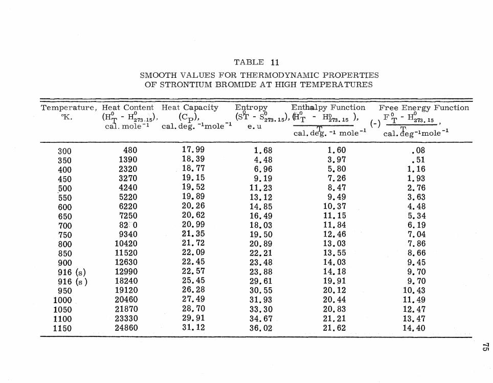
TABLE 11

SMOOTH VALUES FOR THERMODYNAMIC PROPERTIES OF STRONTIUM BROMIDE AT HIGH TEMPERA TURES

Temperature, Heat Content Heat Capacity Entropy Enthalpy Function Free Energy Function °K. (H~ - H~73 _15), ( cP), _ (sir - s~73 • 15), (H; - Hg73 • 15 ), FT - H~73 • 15

300 350 400 450 500 550 600 650 700 750 800 850 900 916 (s) 916 (s) 950

1000 1050 1100 1150

cal.mole-1 cal.deg. -1 mole 1 e.u T 1 (-) ;I; ' cal. deg. - 1 mole- cal. eg-lmole -l

480 1390 2320 3270 4240 5220 6220 7250 82 0 9340

10420 11520 12630 12990 18240 19120 20460 21870 23330 24860

17.99 18.39 18.77 19.15 19. 52 19.89 20.26 20.62 20.99 21.35 21. 72 22.09 22.45 22.57 25.45 26.28 27.49 28.70 29.91 31.12

1. 68 4.48 6.96 9.19

11. 23 13.12 14.85 16.49 18.03 19.50 20.89 22.21 23.48 23.88 29.61 30.55 31. 93 33.30 34.67 36.02

1. 60 3.97 5.80 7.26 8.47 9.49

10.37 11.15 11.84 12.46 13.03 13.55 14.03 14.18 19.91 20.12 20.44 20.83 21.21 21. 62

• 08 • 51

1. 16 1. 93 2.76 3.63 4.48 5.34 6.19 7.04 7.86 8.66 9.45 9.70 9.70

10.43 11. 49 12.47 13.47 14.40

-l CJl

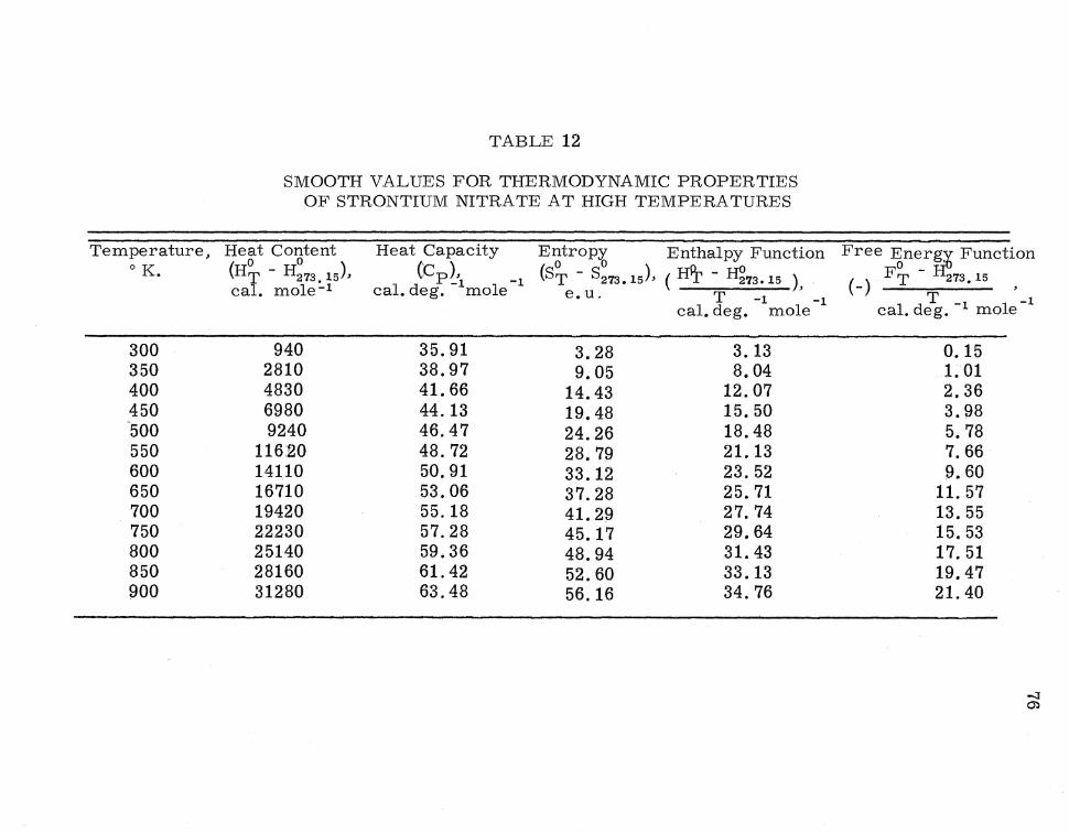
TABLE 12

SMOOTH VALUES FOR THERMODYNAMIC PROPER TIES OF STRONTIUM NITRATE AT HIGH TEMPERATURES

Temperature, Heat Content o K. (H; - H~73. 15),

cal. mole- 1

300 940 350 2810 400 4830 450 6980 -500 9240 550 11620 600 14110 650 16710 700 19420 750 22230 800 25140 850 28160 900 31280

Heat Capacity Entropy Enthalpy Function Free Ener~ Function

(CP~'1 -1 (s; - s~73. 15), ( Hit, - H~73.15 ), (-) F; - 273, 15 , cal. deg. mole e. u. T _1 _1 T _1

cal. deg. mole cal. deg. - 1 mole

35.91 3.28 38.97 9.05 41. 66 14.43 44.13 19.48 46.47 24.26 48.72 28.79 50.91 33.12 53.06 37. 28 55.18 41. 29 57.28 45.17 59.36 48.94 61.42 52.60 63.48 56.16

3.13 8.04

12.07 15.50 18.48 21.13 23.52 25.71 27.74 29.64 31.43 33.13 34.76

0.15 1.01 2.36 3.98 5.78 7.66 9.60

11. 57 13.55 15. 53 17.51 19.47 21. 40

-:J Cl)

CHAPTER IX

DISCUSSION

1. Relation to Previous Work

Neither strontium bromide nor strontium nitrate had been

studied extensively by calorimetric means before this investiga­

tion. However two investigators have obtained mean heat capacity

values over certain temperature intervals, and these literature

values are compared with the results of this investigation in

Table 13. The comparisons were made by interpolating the

tabulated heat capacities at the proper temperature intervals.

In the alkaline earth family of nitrates, the low tempera-

ture heat capacities of magnesium, calcium, and barium were

l studied by Shomate and Kelley. As shown in Table 14 a compari-

son of the heat capacities and entropies of the alkaline earth

nitrates at 298.15° K. indicates that both heat capacity and entropy

increase as the atomic weight of the cation increases.

2. Scatter

The scatter of the data in both high and low temper.ature

work is small and substantially random. Only a few measure-

1C. H. Shomate, and K. K. Kelley, J. Am. Chem. Soc., 66., p. 1490 (1944).

77

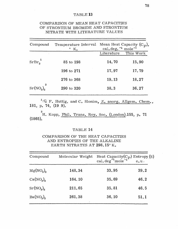
TABLE13

COMPARISON OF MEAN HEAT CAPACITIES OF STRONTIUM BROMIDE AND STRONTIUM

NITRATE WITH LITERATURE VALUES

78

Compound Temperature Interval Mean Heat Capacity (Cp), cal. deg. ':"l mole-1 o K.

Literature This Work

SrBr2 1

85 to 198 14.70 15.90

196 to 271 17.97 17.79

276 to 368 19.13 18.27 2

Sr(NO3) 2 290 to 320 38.3 36.27

1(Ci F. Huttig, and C. Slonim, z. anorg. Allgem. Chem., 181, p. 74, (19. 9).

2

H. Kopp, Phil. Trans. Roy. Soc. (London),155, p. 71 (1865).

TABLE 14

COMPARISON OF THE HEAT CAPACITIES AND ENTROPIES OF THE ALKALINE

EARTH NITRATES AT 298.15° K.

Compound Molecular Weight Heat Capacity(Cp) Entropy,(S) -1 -1 cal. deg mole e. u.

Mg(NO3 ) 2 148.34 33.95 39.2

Ca(NO3 ) 2 164.10 35.69 46.2

Sr(NO3 ) 2 211. 65 35.81 46.5

Ba(NO3) 2 261. 38 36.10 51.1

79

ments obtained with the low temperature calorimeter deviate

from a smooth curve drawn through the data points by more than

0. 2 per cent. The standard errors for single values calculated

from the equations selected to represent the high temperature

heat content data amount to only about O. 4 calories per gram.

Errors in the low temperature measurements could be

caused by three factors: (1) transfer of heat to or from the

sample container, (2) errors in measurement of energy input,

(3) errors in measurement of the temperature rise. Transfer

of heat to the sample container might occur by conduction of heat

along the copper lead wires or nylon string support, by convec­

tion currents in the rarified atmosphere, or by interchange of

radiant energy with the adiabatic shield. The lead wires were

wrapped around the adiabatic shield several times and painted

with varnish to insure good thermal contact with the shield. Ac -

curate regulation of the shield temperature could therefore

minimize both conduction and radiation. The shield control

circuit enabled the detection of as little as 0. 3 microvolts gener­

ated by a difference thermocouple between the shield and sample

container. This voltage corresponds to about 0. 02° K. at 60° K.

or 0. 008° K. at 300° K. for the copper constantan couple used.

Energy input measurements depended on the accuracy of the

potentiometer and precision resistors used in the electrical

80

circuits and on the accuracy of the sychronous timer used to

measure the time of energy input. The potentiometers and

resistors had been calibrated and were considered accurate

to 0. 05 per cent or better:;>. the timer, however, depended on

the accuracy of the 60 cycle alternating current. Fluctuations

in the line frequency might therefore cause significant errors

in the heat capacity measurements. The temperature before

and after heating was measured with a platinum resistance

thermometer and a Mueller bridge, both of which had been cali­

brated by the National Bureau of Standards. Information re­

ceived with the thermometer and bridge calibration certificates

indicated that a temperature rise of about 5 degrees could be

measured accurately to 0. 001 degree. At 60° K., an error

of 0. 001 degree in a 5 degree temperature rise corresponds

to an error of less than 0. 05 per cent in the heat capacity

measurements.

The standard errors obtained from high temperature

enthalpy measurements (about O. 4 calories per gram) were ap­

proximately constant regardless of the temperature range

covered. Experimentation identified the major cause of error

in the high temperature enthalpy measurements as the mercury

handling system of the Bunsen ice calorimeter. An error of '

0. 4 calories per gram could be caused by a change in volume

81

of the mercury system of only 0. 005 ml. The operation of the

valve in the mercury line could easily cause a change in volume

of this magnitude.

3. Summary and Conclusions

A low temperature adiabatic calorimeter was designed, con­

structed, and operated. The operation of the calorimeter was

tested and proved satisfactory by measuring the heat capacity of

a sample of benzoic acid obtained from the National Bureau of

Standards. These measured heat capacity values were compared

with similar values obtained by the Bureau of Standards, and they

agreed within + 0. 5 per cent. After the accuracy was checked

the calorimeter was used to measure the heat capacities of

strontium bromide and strontium nitrate from 60 to 300° K. The

heat capacity data were extrapolated to 0° K. with the method used

2 by Kelley and smooth values of heat capacity, entropy, enthalpy

O O 0 function HT - Hg , and free energy function FT - H0 were cal-

T T culated and tabulated at even 10-degree intervals.

Enthalpy measurements were made on strontium bromide

at temperatures ranging from 300 to 1150° K. and on strontium

nitrate from 300 to 900° K. using a Bunsen ice calorimeter.

2K. K. Kelley, Contributions to the Data on Theoretical Metallurgy. U. S. Bureau of Mines Bull. 477, 137 p., (1950).

82

The enthalpy data were fitted with algebraic equations by applying

the method of least squares; calculations of values of heat capacity,

entropy, enthalpy function, and free energy function were made

at even 50-degree temperature intervals. The heat and entropy

of fusion of strontium bromide were calculated from the enthalpy

measurements.

The largest source of error in the entropy and thermodynamic

functions calculated for the strontium compounds is probably the

error in the extrapolated portion of the heat capacity curve. All

of the low temperature measurements should be extended to liquid

helium temperatures to eliminate this error. Based on measure­

ments with benzoic acid, the heat capacity measurements should

be within+ O. 5 per cent of the true values.

BIBLIOGRAPHY

BIBLIOGRAPHY

BOOKS

Archibald, E. H., The Preparation of Pure Inorganic Substances. New York: John Wiley & Sons, Inc., 1932.

Booth, S. F. , Precision Measurement and Calibration, Selected Papers on Heat and Mechanics., Vol. 2. National Bureau of Standards Handbook 77., 1961.

Glasstone., S., Textbook of Physical Chemistry, 2nd ed. New York: D. Van Nostrand Co • ., Inc., 1946.

_____ . Thermodynamics for Chemists. New York: D. Van Nostrand Co., Inc., 1947.

Kelley, K. K., Contributions to the Data on Theoretical Metal­lurgy. U. S. Bureau of Mines Bulletin 477., 1950.

Mellor, J. W. , A Comprehensive Treatise on Inorganic and Theoretical Chemistry, Vol. 3. New York: Longmans, Green., & Co., 1946.

Roth, W. A. and K. Schell., eds • ., Landolt - Bornstein Physikalisch-Chemische Tabellen., 1st supp. Berlin: Verlag von Julius Springer., 1927.

PERIODICALS

Born., M • ., and T. von Karman., rrTheory of Specific Heats., rr Phys. Zeit., 14:15-19, 1913.

Debye, P • ., rrzur Theorie der Spezifischen Warmen., rr Annalen der Physik., 39 :789-839, 1912.

Einstein., A • ., rrPlanck' s Theory of Radiation and the Theory of Specific Heats, rr Ann. Phys. (4) 22:180-190., 1907.

Furukawa., G. T • ., R. E. Mccoskey., and G. J. King, rrca:lorimetric Properties of Benzoic Acid from 0° to 410° K • ., n J. Res. N. B. S • ., 47:256-261, Octe>ber., 1951.

84

85

Furukawa .. G. T ... T. B. Douglas .. R. E. Mccoskey, and D. C. Ginnings., rrThermal Properties of Aluminum Oxide from 0° to 1200° K ... tr J. Res. N. B. S. 57:67-82, August .. 1956.

Gibson .. G. E ... and Giauque .. W. F. riThe third law of thermo­dynamics. Evidence from the specific heats of glycerol that the entropy of a glass exceeds that of a crystal at the absolute zero, ir Jour. Am. Chem. Soc., 45: 99 .. 1923.

Huttig, C. F., and C. Slonim .. rrDie Spezifischen Warmen., Bildungswarmen und Zersetzungsdrucke der Strontium­ha1ogenidp:ydrate, tr z. anorg. und allgem. Chem ... 181: 65-77,1929.

Kopp., H. "Investigations of Specific Heat of Solid Bodies .. n

Phil. Trans. Roy. Soc. (London) .. 155:71 .. 1865.

Lewis .. G. N . ., and G. E. Gibson .. "Entropy and the Third Law of Thermodynamics., 11 J. Am. Chem. Soc., 39:2554-81, 1917.

Maier .. C. G. and K. K. Kelley .. ttAn Equation for the Presen­tation of High Temperature Heat Content Data, tr J. Am. Chem. Soc • ., 54: 3243 .. 1932.

Millar., R. W • ., rrThe Specific Heats at Low Temperatures of Manganous Oxide, Manganous-manganic oxide and Manganese Dioxide, n J. Am. Chem. Soc ... 50:1875-1883 .. 1928.

Nernst, W ., and F. Schwers, ninvestigations of Specific Heats at Low Temperatures, n Sitzb. Konig., Preuss. Akad. Wiss., 1914.

Nernst, W. , and F. A. Lindemann, ttspezifische Warme und Quantentheorie, 11 Zeit. fur Electrochem., 17:817-833, 1911.

Rebens, H. and H. Nolnogel, irinvestigations with Infra-red Rays of Great Length, ,r Phil. Mag., 19:761-771, 1910.

Ruehrwein, R. A., and H. M. Huffman, rrA New Method of Heat Transfer in Low Tempe:t?ature Calorimetry, ir J. Am. Chem. Soc., 65:1620-1624, 1943.

86

Shomate, C. H. , and K. K. Kelley, ir The Specific Heats at Low Temperatures of Nitrates of Magnesium., Calcium., Berium., and Aluminum., n J. Am. Chem. Soc., 66:1490-1492, 1944.

DOCUMENTS AND MANUSCRIPTS

Kaylor, C. E., Heat Capacities at High Temperatures, a disserta­tion, University of Alabama., 1958.

Walden., G. E • ., The NaF -RbF System at High Temperatures., a dissertation., University of Alabama., 1959.