Embed Size (px)
Citation preview
THE ANALYSIS AND INTERPRETATION
OF HIGH RESOLUTION
NUCLEAR MAGNETIC RESONANCE SPECTRAby 4T. OF TECHN
by JUL 16 1958Richard Warren Fessenden ' IR RA
B.S., University of Massachusetts(1955)
SUBMITTED IN PARTIAL FULFILLMENT
OF THE REQUIREMENTS FOR THE
DEGREE OF DOCTOR OF
PHILOSOPHY
at the
MASSACHUSETTS INSTITUTE OF TECHNOLOGY
June, 1958
Signature
Certified
of Author
by
Department of Chemistry, May 16, 195d
Th silg STpervisor
Accepted byCha man, Depitmenfalf Committee
on Gradua /Students
I- " ~ ` ~'~Tm` w W

This thesis has been examined by:
Thesis~ommi~ttee Chairman
SThesis ommittee Chairman
Thesis Supervisor
MCI'V V- , o, V
3
THE ANANLYSIS AND INTERPRETATION OF
HIGH RESOLUTION NUCLEAR MAGNETIC RESONANCE SPECTRA
by
Richard Warren Fessenden
Submitted to the Department of Chemistry
on May 16, 1958
in Partial Fulfillment of the Requirements
for the Degree of Doctor of Philosophy
ABSTRACT
The high resolution nuclear magnetic resonance spectraof three ompounds containing three nonequivalent spin 1/2nuclei (H ) have been observed at several magnetic fieldstrengths. The compounds studied were styrene, 2,4-dichloro-aniline and 2,5-dichloroaniline. The spectra, which departconsiderably from first order behavior, have been analyzedand it was found that the sam.e set of parameters describethe spectra at all the magnetic fields used. Using thesecompounds, combination lines have been observed for thefirst time and it was demonstrated that these lines arenot always of small intensity, as had been commonly supposed.It was shown that in styrene the spin-spin coupling constantshave the same sign.
Methods were developed which aid greatly in the analysisof spectra of systems of three spins, when these spectrashow the results of intermediate coupling between the nuclei.
A Using these methods it is possible, in favorable cases, todetermine the relative signs of the coupling constantswithout a complete analysis.
Two substituted ethanes, CHCIBrCBrF2 and CHCI CC1Fwere studied; the spectra were found to exhibit the effectsSof internal rotation. The temperature dependences ofcertain chemical shifts and spin-spin couplings weremeasured, and an attempt made to interpret them in termsof the simple theory of rotational averaging which hasappeared in the literature.
Thesis Supervisor: John S. Waugh
Title: Assistant Professor ofChemistry

ACKNOWLEDGEMENTS
It is with great pleasure that I acknowledge the
guidance of Prof. John S. Waugh during the course of
this research. His help in selecting the problem,
opportune suggestions regarding both the work in
progress and that contemplated, and leadership in
many inspiring discussions made the research pleasant,
stimulating and productive.
I am grateful for the many opportunities of
discussing the three-spin problem with Dr. Salvatore
Castellano, for the many discussions with Dr. Donald
M. Graham, and for the latter's pioneering efforts
with the thermostat. I would also like to express
my appreciation to those who have already left the
laboratory for leaving much experimental "lore",
and to those who are still here for helping me to
realize the value of perpetuating it. I am grateful,
too, to my wife for her help in preparing the manuscript.
I wish to thank both the National Science Foundation,
for their fellowship support, and the directors of the
Research Laboratory of Electronics, for making the
Laboratory's facilities available for this research.
TABLE OF CONTENTS
I. Introduction: Spectra of Three-Spin Systems ...
II. Theory of the Case ABC.........
III. Experimental ...................
IV. Results and Discussion.........
V. Conclusion......................
VI. Introduction: Internal Rotation
VII. Theory of Rotational Averaging.
VIII: Theory of the Case ABX..........
IX. Experimental...................
X. Results and Discussion..........
XI. Conclusion......................
Appendix A .......................
Appendix B ........................
Literature Cited ..................
........ 7
..11
S.33
.. 38
*.59
. .61
.. 62
.. 69
* .73
•.79
.. 88
..90
- .95
.103
........
LIST OF FIGURES
First Order Spectrum for ABC ........
Spectrum of Styrene, 40 Mc..........
.................. ...20
..................... 39
1.
2.
3.4.
5.6.
7.8.
9.10.
11.
12.
13.
14.
.40
.44
.45
.48
.51
.56
.72
.76
Two Alternate Calculated Spectra for Styrene
Spectrum of Styrene, 22.55 Mc................
Spectrum of Styrene, 10 Mc ..................
Correlation Diagram for Styrene..............
Spectra of 2,4-Dichloroaniline..............
Spectra of 2,5-Dichloroaniline ..............
Spectrum Calculated for ABX = F 1 F 2 H.........
Thermostat for Rotating Sample...............
Spin-Spin Coupling Constant in CHC12CC1F 2
vs. Temperature...................
AHF in CHC12CC1F 2 vs. FB, EB - EA 0........AHF in CHC1 2CC1F2 vs. FB, EB - EA( 0........
VF2 - V at 40 Mc. in CHClBrCBrF2 vs. Tempei
15. The Two H-F Spin-Spin Couplings in CHClBrCBrF 2vs. Temperature ............................. ...... 86
LIST OF TABLES
Matrix Elements of Y ........................First Order Transitions -i j..............The Aij as They Appear in a First Order Spectrum.
Styrene, 40 Mc....................................
Styrene, 22.55 Mc. and 10 Mc.....................
2,4 -Dichloroaniline, 40 Mc. and 22.55 Mc..........
2,5-Dichloroaniline, 40 Mc. and 22.55 Mc..........
Energy Levels for the Case ABX...................
.14
.18
.21
.42
.46
.53
.57
.70
............. 80
....... ....... 82
....... ....... 83
rature.......85
i.
II.
III.
IV.
V.
VI.
VII.
VIII.
I. INTRODUCTION: SPECTRA OF THREE-SPIN SYSTEMS
The Hamiltonian used to describe the fine structure
in the nuclear magnetic resonance spectra of liquid and
gaseous samples was proposed by Hahn and Maxwell (17) and
by Gutowsky et al. (16), and has been justified by Ramsey
(32, 33) and Ramsey and Purcell (34). There are two
kinds of effects involved: shielding of the nucleus from
the external magnetic field by induced electron currents
and orientation-independent coupling of pairs of magnetic
nuclei by the electrons. The Hamiltonian describing these
two effects can be written(0) 1(/,)
where --(0) _ itiHiizi (1)
and -1 -Z 2Aii
Here'r has the usual significance, Ti is the magnetogyric
ratio of nucleus i, Hi the magnetic field at nucleus i,
Izi the z component of the spin angular momentum, Aij a
coupling constant, and I. and I. the spin angular momenta.()-i (1)
ýV(O) is dependent upon magnetic field while j) is not,
because A.. is assumed to be independent of magnetic
field, as predicted by Ramsey and Purcell (34). There
is good experimental and theoretical justification (32)
for assuming Hi to be of the form Ho(1-%i), that is,
linear in the external field. The Ai for some selected
compounds have been shown to be independent of magnetic
field between the values 200--6000 gauss, to within the
experimental error of approximately 10/o (31, 16). Over
the temperature range studied by Gutowsky et al. (16), no
change in the values Aij were detected. The dependence
of Hi on magnetic field and the independence of Aij
can be assumed until refuted by some more sensitive
method of measuring the effects by which Hi ( i) and
A.. are manifest. The work described herein deals with13
this question only indirectly.
The ability of the Hamiltonian to describe the
positions of lines and their intensities -- the observable
features of a magnetic resonance spectrum -- has been
tested in many cases. If
2wAij <<
IYHi-HjI
for all pairs of nuclei, then the interpretation is simple:
a first order perturbation treatment is sufficient, and
it has always been possible to determine a set of para-
meters, the i andAij, which adequately describes the
experimental spectra.
Some simple cases where first order theory is not
adequate have been investigated. Following the notation
used by Bernstein, Pople, and Schneider (7), nuclei i and
j for which .\. Y 1 will be denoted by the first letters13
of the alphabet A,B,C---; nuclei i, for which .ij<< 1
with all others j, will be called by other letters, such
as P, X, or Y. In this notation, three nuclei with only
1-2 1 would be called ABX. Systems AB (17), AB n with
n = 2,3,4 (6), and A2X2 (24) have been treated exactly.
Some other systems have been discussed (7, 15, 20, 30),
but the results are not easily presented in closed form.
One of these systems is ABX, which has been treated by
Bernstein, Pople, and Schneider (7) and Gutowsky et al.
(15). This is a special case of the general system of
three nuclei which will be treated in detail in section II.
A perturbation treatment has also been presented (2) for
cases in which the N.. are appreciable but still lessthan unity. Here the perturbation is expanded in terms
than unity. Here the perturbation is expanded in terms
of the -'s, and in one case (4) it has been carried out
to third order. In all cases it has been possible to get
satisfactory agreement between theory and experiment, and
the parameters a. and A.. have been obtained.1 ijThe case of three non-equivalent nuclei, ABC, is
more complicated than those previously mentioned, and
it is quite worthwhile to determine for this case whether
satisfactory agreement with experiment exists when the
values of >i approach unity or even exceed it. Here
the perturbation treatment may not be valid because there
is a possibility that the series in the A's will not
converge. In fact, the three-spin system is the simplest
one in which it is possible that neither a series in A
nor one in 1/? will converge.
For one to be able to interpret the spectra of three-
spin systems conveniently, the spectra cannot depart greatly
from those in which a first order theory is appropriate.
If this is true, the three hij are significant but not
large, and the case does not present a difficult enough
test to the theory. It is possible, however, to analyze
a spectrum taken at a higher magnetic field (in which
some A• 1/2) and then to take a spectrum at a lower
magnetic field, where the A's are larger. If the same
set of parameters is assumed to hold at the lower field
and the spectrum calculated on that basis agrees with
experiment, then the theory has been put to a significant
test (A r 2) and has withstood that test.
The spectra at several magnetic fields can be used
at the same time to verify that the same set of parameters,
ai and Aij, describes the spectrum at different magnetic
fields. This relates to the dependence of Hi and Aij on
magnetic field, but the proper dependence has been shown
previously only for cases in which all .ij(l.
10
Systems containing three or more spins are of particular
interest because of some additional properties of their
spectra. As Anderson (2) has mentioned, in this case it
is possible to determine the relative signs of the three
or more Aij, although the absolute signs can never be-ijdetermined (Appendix A). Several theories (16, 21, 33)indicate that for protons all the coupling constants
should be positive; however, one paper has appeared in
the literature (1) in which the author claims to have
found an instance in which all the proton couplings are
not of the same sign. Since it has been possible to find
the signs of the A's in very few cases, it is important
to do so in more cases in order to verify or reject theories
of their origin.
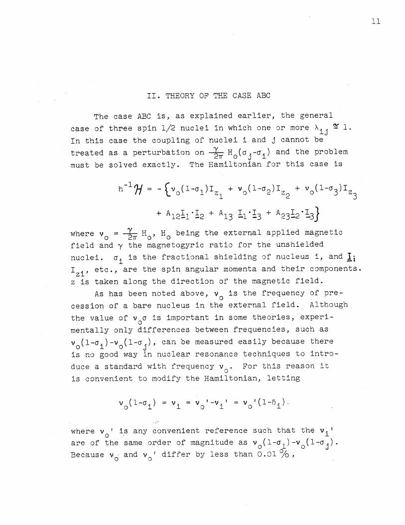
II. THEORY OF THE CASE ABC
The case ABC is, as explained earlier, the general
case of three spin 1/2 nuclei in which one or more ij .In this case the coupling of nuclei i and j cannot be
treated as a perturbation on -- H (a• - i ) and the problem
must be solved exactly. The Hamiltonian for this case is
h- 1J= - (v1-al1) + V (l-ai,)I + v (1-C )Iz
12 Z1 2 13 1 3+ A1211 *12 + A13 L1 i 3 + A2312131
where v = -•- H, H being the external applied magnetic0 27 o0 o
field and y the magnetogyric ratio for the unshielded
nuclei. ai is the fractional shielding of nucleus i, and Ji
Izi , etc., are the spin angular momenta and their components.
z is taken along the direction of the magnetic field.
As has been noted above, vo is the frequency of pre-
cession of a bare nucleus in the external field. Although
the value of v a is important in some theories, experi-
mentally only differences between frequencies, such as
vo(1-i)-Vo(l-oj), can be measured easily because there
is no good way in nuclear resonance techniques to intro-
duce a standard with frequency v0 . For this reason it
is convenient to modify the Hamiltonian, letting
v (1- v = V '-v.' = V '(1-5i)
where vo ' is any convenient reference such that the vi '
are of the same order of magnitude as v (l-oi)-vo(l- 1).
Because v and v ' differ by less than 0.01 %,/oBecus Oo adv
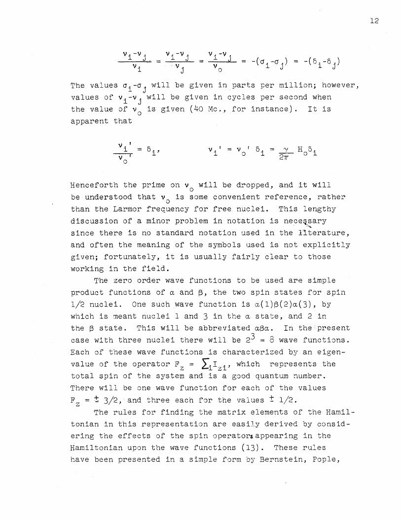
12
V -v . V.-V vL-v ( )
Vi V. V 1 3 11i 0
The values .i-aj will be given in parts per million; however,
values of vi-v j will be given in cycles per second when
the value of v is given (40 Mc., for instance). It is
apparent that
V. Si , V.= 5 = V Ho5t 1 1 0 1 o0v 27
Henceforth the prime on vo will be dropped, and it will
be understood that vo is some convenient reference, rather
than the Larmor frequency for free nuclei. This lengthy
discussion of a minor problem in notation is neceQsary
since there is no standard notation used in the literature,
and often the meaning of the symbols used is not explicitly
given; fortunately, it is usually fairly clear to those
working in the field.
The zero order wave functions to be used are simple
product functions of a and D, the two spin states for spin
1/2 nuclei. One such wave function is a(l)ý(2)a(3), by
which is meant nuclei 1 and 3 in the a state, and 2 in
the ý state. This will be abbreviated a8a. In the'present
case with three nuclei there will be 2 = 8 wave functions.
Each of these wave functions is characterized by an eigen-
value of the operator Fz = I i , which represents the
total spin of the system and is a good quantum number.
There will be one wave function for each of the values
Fz = t 3/2, and three each for the values ± 1/2.
The rules for finding the matrix elements of the Hamil-
tonian in this representation are easily derived by consid-
ering the effects of the spin operatorsappearing in the
Hamiltonian upon the wave functions (13). These rules
have been presented in a simple form by Bernstein, Pople,
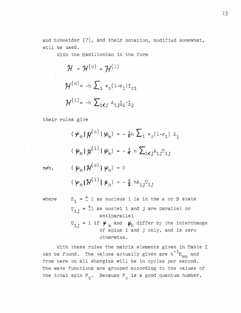
13
and Schneider (7), and their notation, modified somewhat,
will be used.
With the Hamiltonian in the form
(o) -h vo(1-al)Izi
(1)= h i(j A.I.*I..
their rules give
(o) m = - Ih vi(1-cli) S i
("m (1) m):= - h Zi<jAijTij
(Y (I1)I(n) I hA.UL.
where Si =+ 1 as nucleus i is in the a or $ state
Tij = + as nuclei i and j are parallel orTij
antiparallel
Ui. = 1 if m and Kn differ by the interchange
of spins i and j only, and is zero
otherwise.
With these rules the matrix elements given in Table I
can be found. The values actually given are h -H m n and
from here on all energies will be in cycles per second.
The wave functions are grouped according to the values of
the total spin F . Because FZ is a good quantum number,z
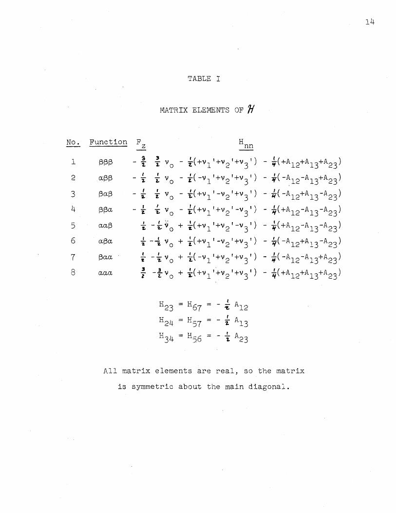
TABLE I
MATRIX ELEMENTS OF
Function
Ba$
Bpa
maa
apa
Baa '
maa
F
3
3-i
I
3
3t V
v 0
V 0o0
V o
3 oE V! o
H23H2 4
H314
Hnn
- {(+v 1 +v2 + 31')
- (-v 1 '+v2 +v )
+1 2 3(+v '-v '+v ')(+ 1 2 3
- 1 '+v I -V )+ j(-v 1 2'+ 31)
+ t(+v l' -v 2 +v3 ')
+ (-'+v '+v ')+L(vl 2 3+ -(+v1 '+v '+v ')-- 1 2 3
H A67 - 12
H P57 2• 13
H6 . A23
- #(+A1 2+A13+A23)
- (-A12+A13-A23)
- (+A 12 -A 13 -A2 3)
(-A12 + 13A23)-(+AA +A -A)
-L(+A +A +A2 )q 12 13 23
All matrix elements are real, so the matrix
is symmetric about the main diagonal.
No.
1
2
3
4
5
6
7
8
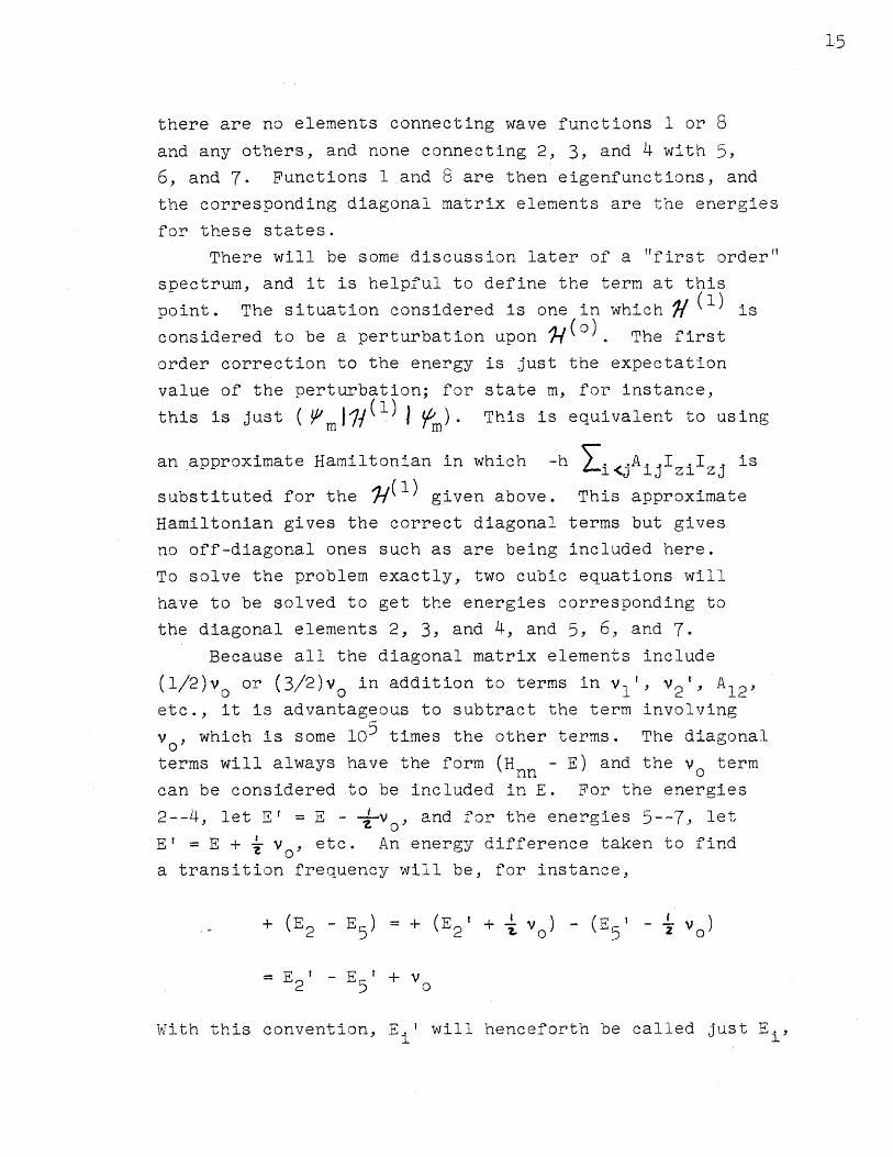
there are no elements connecting wave functions 1 or 8
and any others, and none connecting 2, 3, and 4 with 5,
6, and 7. Functions 1 and 8 are then eigenfunctions, and
the corresponding diagonal matrix elements are the energies
for these states.
There will be some discussion later of a "first order"
spectrum, and it is helpful to define the term at this
point. The situation considered is one in which / (1) is
considered to be a perturbation upon •(o). The first
order correction to the energy is just the expectation
value of the perturbation; for state m, for instance,
this is just ( nmli(1) m) . This is equivalent to using
an approximate Hamiltonian in which -h Ai ziIz is
substituted for the ýY(1) given above. This approximate
Hamiltonian gives the correct diagonal terms but gives
no off-diagonal ones such as are being included here.
To solve the problem exactly, two cubic equations will
have to be solved to get the energies corresponding to
the diagonal elements 2, 3, and 4, and 5, 6, and 7.
Because all the diagonal matrix elements include
(1/2)v or (3/2)v in addition to terms in v1j, V2 A1 2 ,
etc., it is advantageous to subtract the term involving
v , which is some 105 times the other terms. The diagonal
terms will always have the form (H - E) and the v termnn o
can be considered to be included in E. For the energies
2--4, let E' = E - -v, and for the energies 5--7, let
E' = E + - v , etc. An energy difference taken to find
a transition frequency will be, for instance,
+ (E2 - g) (E + (2 j ) - (E5' - V)
E2' - E5 o
With this convention, E.' will henceforth be called just E i ,
!
16
and it will be understood that the value of v should be
included.
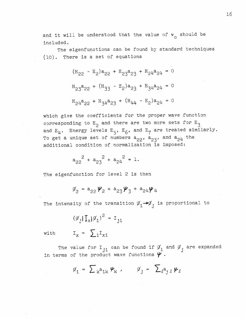
The eigenfunctions can be found by standard techniques
(10). There is a set of equations
(H22 - E2)a 2 2 + H2 3 a 2 3 + H2 a 2 4 = O0
H2 3 a 2 2 + (H3 3 - E2)a 2 3 + H3 4 a 2 4 = 0
H24a22 + H3 4a2 3 + (H4 4 - E2 )a24 = 0
which give the coefficients for the proper wave function
corresponding to E2 and there are two more sets for E3
and E 4 . Energy levels E 5 , E6 , and E7 are treated similarly.
To get a unique set of numbers a2 2 , a2 3 , and a24 the
additional condition of normalization is imposed:
2 2 222 + a23 + 24 =1.
The eigenfunction for level 2 is then
2 = a22 2 + a 2 3 Y 3 + a24?4
The intensity of the transition pi--.j is proportional to
with I x = ixi
The value for I ji can be found if i and .j are expanded
in terms of the product wave functions .
Si Z kZaik Zk j = ,aj p
I
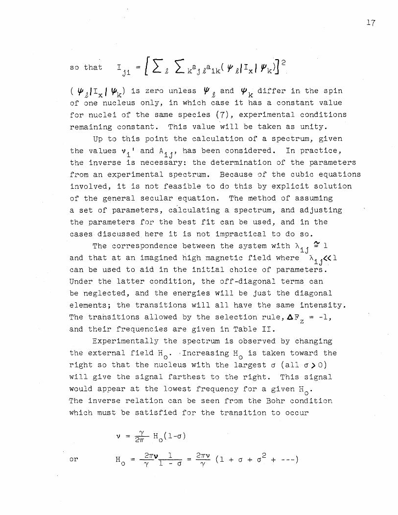
so that i = fZ, jka. 2 a ik( 4 Ix k l 2
( J(Ixl Yk) is zero unless V1, and (k differ in the spinof one nucleus only, in which case it has a constant value
for nuclei of the same species (7), experimental conditions
remaining constant. This value will be taken as unity.
Up to this point the calculation of a spectrum, given
the values v. ' and Ai , has been considered. In practice,
the inverse is necessary: the determination of the parameters
from an experimental spectrum. Because of the cubic equations
involved, it is not feasible to do this by explicit solution
of the general secular equation. The method of assuming
a set of parameters, calculating a spectrum, and adjusting
the parameters for the best fit can be used, and in the
cases discussed here it is not impractical to do so.
The correspondence between the system with A 1
and that at an imagined high magnetic field where ..<<((l13
can be used to aid in the initial choice of parameters.
Under the latter condition, the off-diagonal terms can
be neglected, and the energies will be just the diagonal
elements; the transitions will all have the same intensity.
The transitions allowed by the selection rule, AF = -1,
and their frequencies are given in Table II.
Experimentally the spectrum is observed by changing
the external field Ho . Increasing H is taken toward the0 0
right so that the nucleus with the largest a (all a>O)
will give the signal farthest to the right. This signal
would appear at the lowest frequency for a given Ho
The inverse relation can be seen from the Bohr condition
which must be satisfied for the transition to occur
v = H (1-)2w 0
2wv 1 27v 2or H0 -- , = -- (+ + +---)
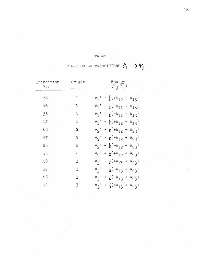
18
TABLE II
FIRST ORDER TRANSITIONSi -- (j
Transitionvji
78
46
35
12
68
47
25
13
58
37
26
14
Origin
v!
v 1
v 1
v 2
v 2
v 2
v 3
v 3
v 3 '
v 313
Energy-(H -H,)
- t(+A + A13)-(-A12 + 13)+ t(-A 2 + A13)
+ -(+A12 + A13)
- •(+A 12 + A23 )
- -(-A12 + A23)+ (-A12 + A23)+ l(+A + A23)
- f(+A13 + A23)- (-A.i + A23)
+ j(-A 13 + A23)+ (+AI3 + A2 3)
S13 23
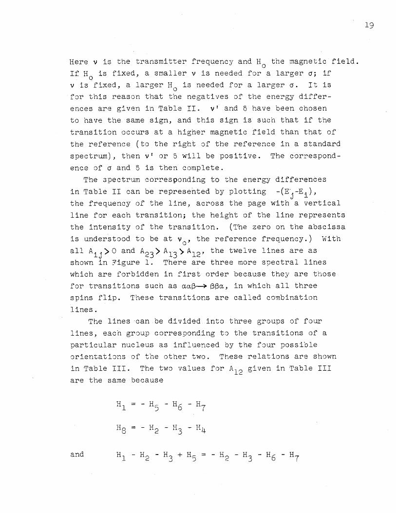
Here v is the transmitter frequency and H° the magnetic field.
If Ho is fixed, a smaller v is needed for a larger a; if
v is fixed, a larger Ho is needed for a larger a. It is
for this reason that the negatives of the energy differ-
ences are given in Table II. v' and 5 have been chosen
to have the same sign, and this sign is such that if the
transition occurs at a higher magnetic field than that of
the reference (to the right of the reference in a standard
spectrum), then v' or 5 will be positive. The correspond-
ence of a and 5 is then complete.
The spectrum corresponding to the energy differences
in Table II can be represented by plotting -(Ej-Ei),
the frequency of the line, across the page with a vertical
line for each transition; the height of the line represents
the intensity of the transition. (The zero on the abscissa
is understood to be at vo, the reference frequency.) With
all AijO and A2 3) A13 A 12 , the twelve lines are as
shown in Figure 1. There are three more spectral lines
which are forbidden in first order because they are those
for transitions such as aa-- ýBý, in which all three
spins flip. These transitions are called combination
lines.
The lines can be divided into three groups of four
lines, each group corresponding to the transitions of a
particular nucleus as influenced by the four possible
orientations of the other two. These relations are shown
in Table III. The two values for Ai2 given in Table III
are the same because
1 = - H5 - HE - H7
H8 = - H2 - 3 - H
and H - H - H3 + H5 = - H2 - H3 - H - H71 2 3 5 2 3 6 7
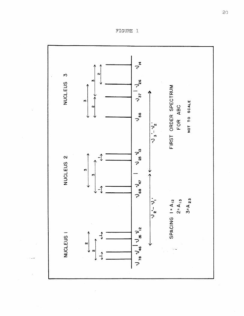
FIGURE 1
-I
-t _________
A1 4 _ _
N~
N
I-~tO
2
(0
InN
co
0 J1 O
O -O o0LLu
cI-LL-
2
2
N t
II II II
()ZO.Q,

TABLE III
THE Ai.. AS THEY APPEAR13
A1 2 = 4 6 - V7 8
v47 - v68
v12 - 351
V13 V25
A1 3 = V3 5 - V7 8 '
v37 - V5 8 IV1 2 - V4 6
V1 4 - V26
A2 3 = 13 - V4 7 1
V1 4 - V37
V2 5 - v 6 8 1V2 6 -v58
= H4
= H
= H1
= H3
- H6
- H2
IN A FIRST ORDER SPECTRUM
H7 + H8
- H3 + H5
- H2 - H4 + H6
- H5 - H7 + H858
H H3 - H4 +HL 3 7
= H2 - H5 - H6 + Hp
Here H1 = H1 1
22
and H4 - Hg - H7 + H8 = - H3 - H6 - H7
therefore H - H2 - H3 + H = H - H - H7 + H8
Similar relations hold for A13 and A23. The spacing
between the centers of two groups of lines will be the
value of v .'-v.J i
It is now possible to show that any spectrum of a
system of three spin 1/2 nuclei is of the same form as
a first order spectrum as far as line positions are concern-
ed; that is, it is possible to find an assignment of lines
into three groups of four lines each, which has the same
property of repeated spacings, although the spacings are
not now just the Aij , but are more complicated functions.
Some other properties of the spectrum will also be investi-
gated which will make possible some statements regarding
the uniqueness of the assignment. To do these things, the
correspondence between the spectrum for all values of ?
and a first order spectrum must be demonstrated.
First it is useful to demonstrate that in the calcula-
tion of the energies from a set of parameters, each energy
can be identified with a particular diagonal element ofN ,in the sense that if the diagonal element and the energy
are observed as functions of magnetic field, in the limit
of infinite magnetic field the two must approach a common
value. In proceeding from parameters to energies, the
identification of the energies with the diagonal elements
can be considered in each of the 3x3 determinants separately.
One factor of the secular determinant is
H 22-E 5H22 5H24
5H23 H33-E H34 = O0
5H24 5H34 H44-E
where 6 is a variable inserted to introduce continuity into
the argument only, and is unity for proper solution of
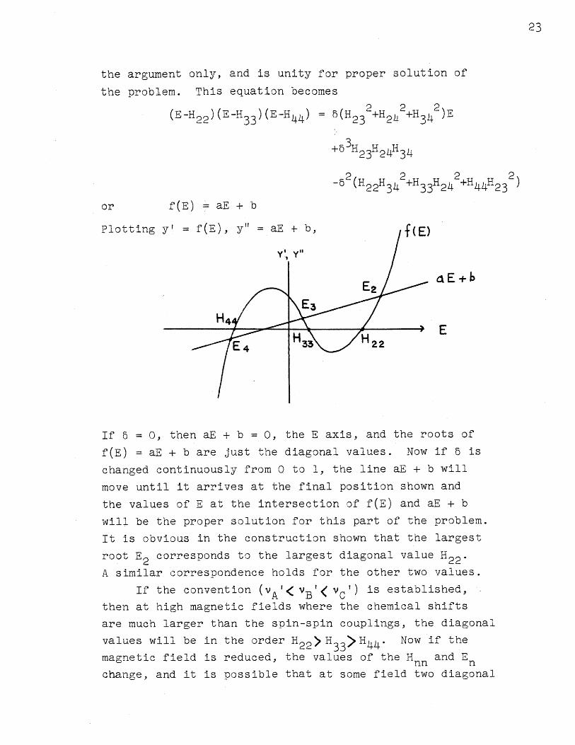
the problem. This equation becomes
(E-H 2 2 )(E-H 3 3 )(E-H 4) = 5(H232+H242+H34 )E
+5 H2 3 H2 4H34
-52 (H22H 2+H33H2 4 2+H44H23)2
or f(E) = aE + bi+- -V N 771l 1 O r
PLUtUU 6L
E+b
E
If 5 = O, then aE + b = O, the E axis, and the roots of
f(E) = aE + b are just the diagonal values. Now if 5 is
changed continuously from 0 to 1, the line aE + b will
move until it arrives at the final position shown and
the values of E at the intersection of f(E) and aE + b
will be the proper solution for this part of the problem.
It is obvious in the construction shown that the largest
root E2 corresponds to the largest diagonal value H22 .A similar correspondence holds for the other two values.
If the convention (vA' VB < V C') is established,
then at high magnetic fields where the chemical shifts
are much larger than the spin-spin couplings, the diagonal
values will be in the order H2 2)H 3 3 H 4 . Now if the
magnetic field is reduced, the values of the Hnn and En
change, and it is possible that at some field two diagonal

24
values, for instance H22 and H33 , can become equal. This
situation is illustrated below by three plots of the
cubic equation for successively smaller magnetic fields.
2 _
E2E3
H33,Ha
E2
H33
In the second diagram it seems meaningless to ask:
to which diagonal value does E2 correspond? However, as
the magnetic field is changed, the energy levels must
change continuously, therefore, the labeling of the roots
is correct as shown in the second and third diagrams.
Even though at the field considered above there is a
change from H2 2 > H3 3 to H22( H3 3 ' E2 remains larger than
E . The only possibility of a change in the order of the
energies is in the case considered above. Because no change
occurred there, the levels must remain in the order
E2 E 3 E4 for all magnetic fields.
2 / _:
-Y
25
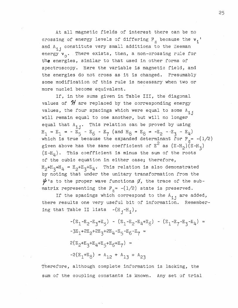
At all magnetic fields of interest there can be no
crossing of energy levels of differing F because the v.'z 1and A.. constitute very small additions to the Zeeman
energy vo. There exists, then, a non-crossing rule for
the energies, similar to that used in other forms of
spectroscopy. Here the variable is magnetic field, and
the energies do not cross as it is changed. Presumably
some modification of this rule is necessary when two or
more nuclei become equivalent.
If, in the sums given in Table III, the diagonal
values of 91 are replaced by the corresponding energy
values, the four spacings which were equal to some Aijwill remain equal to one another, but will no longer
equal that Aij. This relation can be proved by using
H = El = - E5 - E 6 - E 7 (and H 8 = E 8 = -E 2 - E 3 - E 4 )which is true because the expanded determinant for Fz= -(1/2)
given above has the same coefficient of E2 as (E-H2 )(E-H 3 )
(E-H4 ). This coefficient is minus the sum of the roots
of the cubic equation in either case; therefore,
H2+H4+H = E2+E 3+E4 . This relation is also demonstrated
by noting that under the unitary transformation from the
's to the proper wave functions p, the trace of the sub-
matrix representing the F = -(1/2) state is preserved.
If the spacings which correspond to the A.. are added,
there results one very useful bit of information. Remember-
ing that Table iI lists -(H -Hi ),
-(E1-E2-E +E,) - (E1-E 2-E +E) - (E1-E -E 4 ) =
-3E 1 +2E2+2E 3 +2E -E5 - 6 -E =
2(E2+E 3+EE+E +EE6+E) =
-2(E 1 +Eg) = A1 2 + A13 + A2 3
Therefore, although complete information is lacking, the
sum of the coupling constants is known. Any set of trial
[.
26
parameters should take advantage of the sum of the Ai4
in order to reduce the number of parameters which need
to be determined.
In finding the sum of the A's, care must be used
to take the differences v1 2 - 35, etc., in the proper
direction. If, as has been assumed, the A.. are all
positive, the absolute values of the spacings can be
used. There is another procedure which may be simpler.
If a change is made from A12( A1 3 to A12) A13 , it is
obvious from Table II that the inner lines in the group
of four corresponding to nucleus 1 interchange assignment,
while the outer ones remain the same. Because of the
correspondence between the diagonal matrix elements and
the energies, this change in assignment holds whether a
first order spectrum or one in which some Ai• I is
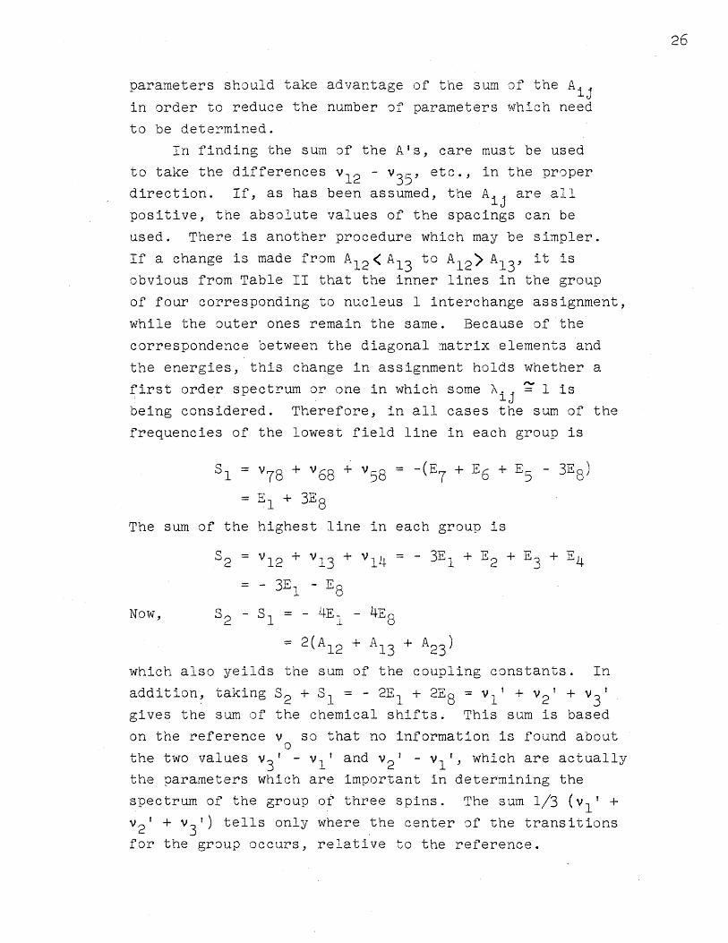
being considered. Therefore, in all cases the sum of the
frequencies of the lowest field line in each group is
SI = 78 + V68 + v58 = -(E7 + E6 + E5 - 3E 8 )
= El + 3E 8
The sum of the highest line in each group is
S2 V1 2 = - 3E + E2 + V1 E + V1 - 3 + E2 E E4
= - 3E1 - E8
Now, S2 - Sl = - 4E1 - 4E8
= 2(A 12 + A1 3 + A2 3)
which also yeilds the sum of the coupling constants. In
addition, taking S2 + Sl = - 2E1 + 2E = v 2 + 3
gives the sum of the chemical shifts. This sum is based
on the reference v so that no information is found about
the two values v3 ' - v1 ' and v' - v 1 , which are actually
the parameters which are important in determining the
spectrum of the group of three spins. The sum 1/3 (vl' +
v2 + v3 ') tells only where the center of the transitions
for the group occurs, relative to the reference.
27
The centers of the multiplet groups may be in the
same order as the vi ', but a more detailed treatment of
the energy levels is necessary to show this (if it is
indeed true), and it has not as yet been possible to
perform such a treatment.
It is useful to sum up what has been found -so far.
Any spectrum of three spins can be broken down into three
groups of four lines, each group corresponding to transi-
tions of a particular nucleus (the word "corresponding"
has been used in the same sense as above, exact identifi-
cation being possible only in the limit of infinite magnetic
field). These three groups of first order lines have the
same property of repeated spacings as in a first order
spectrum. There are, in general, three more lines which
are the combination lines forbidden in first order, but
which become observable in a strongly perturbed case because
of mixing of the wave functions. Not all of these are
usually observable, although one or two often are. The
intensities of the first order lines can very greatly
from unity, and some may not be observable if the \ij are
large. These facts should be remembered in trying to
assign lines in a spectrum.
Some information about the line intensities can be
obtained by considering only the form of the solution
for them. The allowed transitions Fz6 = -1 occur in
three groups: transitions from state 8 to the three 5,
6, and 7, from 2,3, and 4 to 1, and from 5, 6, and 7 to
2, 3, and 4. There are obviously fifteen altogether.
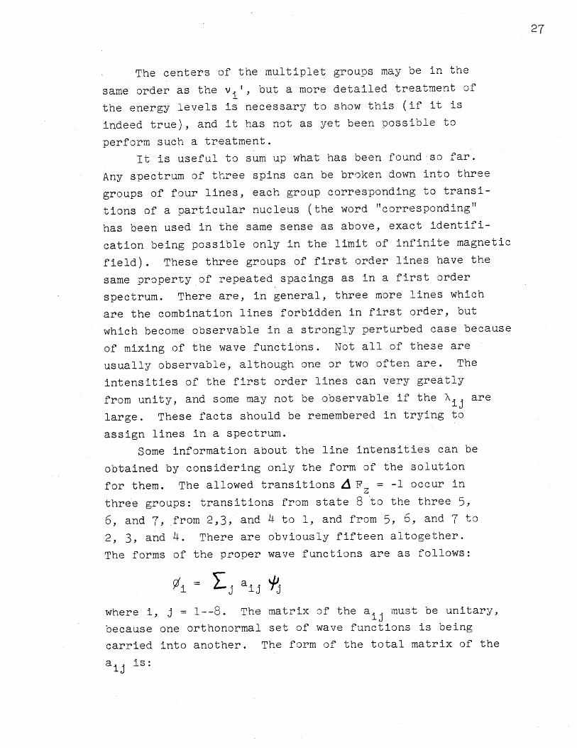
The forms of the proper wave functions are as follows:
i= aiJ aij 'jwhere i, j = 1--8. The matrix of the a. must be unitary,
because one orthonormal set of wave functions is being
carried into another. The form of the total matrix of the
a is:ij
0
(3x3)
(3x3)
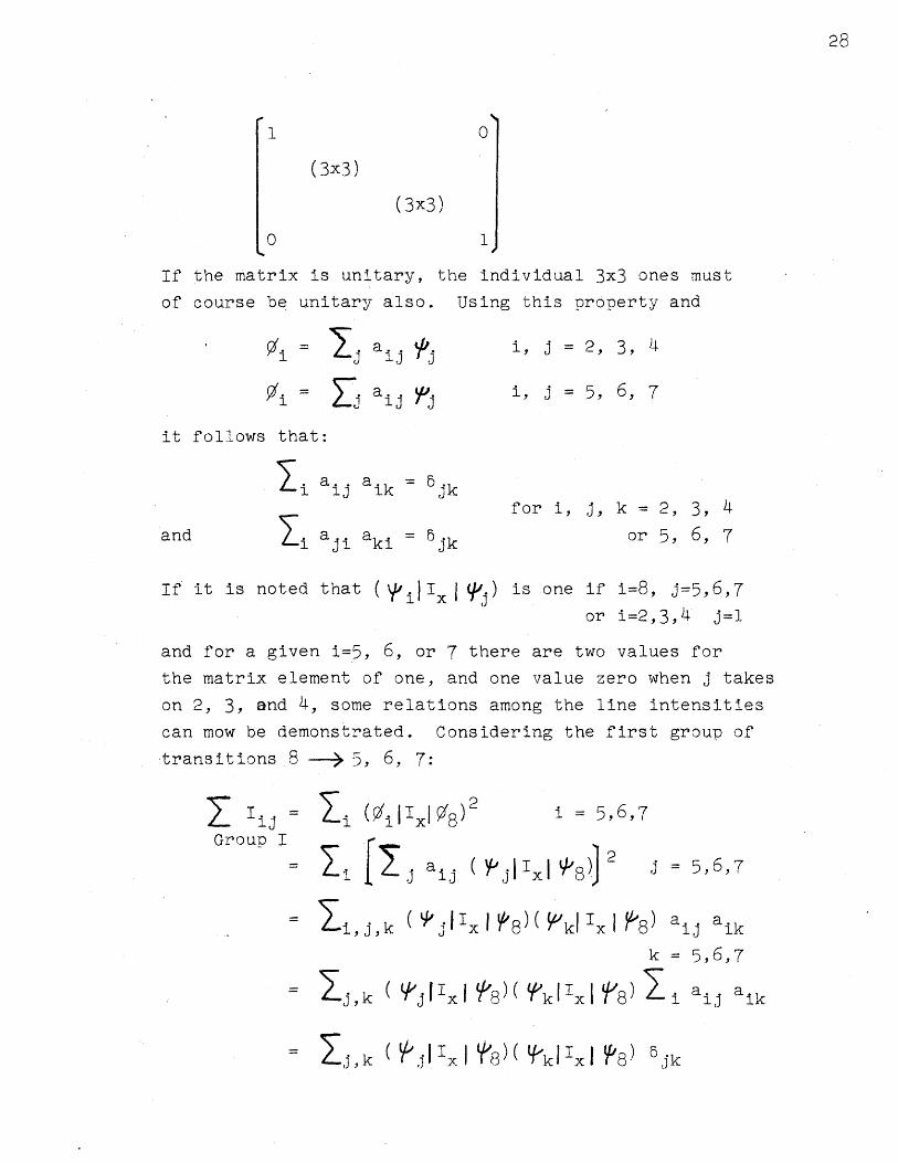
If the matrix is unitary, the individual 3x3 ones must
of course be unitary also. Using this property and
•.i j aij j
=i = aij j
i, J = 2, 3, 4
i, j = 5, 6, 7
it follows that:
1i aij a a = 3jk
and i aji aki = 5 jk
If it is noted that ( ~iIx q3j)
for i, j, k = 2, 3, 4
or 5, 6, 7
is one if i=8, j=5,6,7
or i=2,3,4 j=1
and for a given i=5, 6, or 7 there are two values for
the matrix element of one, and one value zero when j takes
on 2, 3, and 4, some relations among the line intensities
can mow be demonstrated. Considering the first group of
transitions 8 -- 5, 6, 7:
GrouIjGroup I
1i 1ix8 )2 i = 5,6,7
= T aij ( IIx 8) 2 j = 5,6,7
1i,j,k ( 'jIx kI8)(Wk Ix 8) a ikk = 5,6,7
= yj,k ( jI Ix k kIx 8) -i aij aik
= j,k ( L 8 (IkI Ix k 8 jk
28
I
29
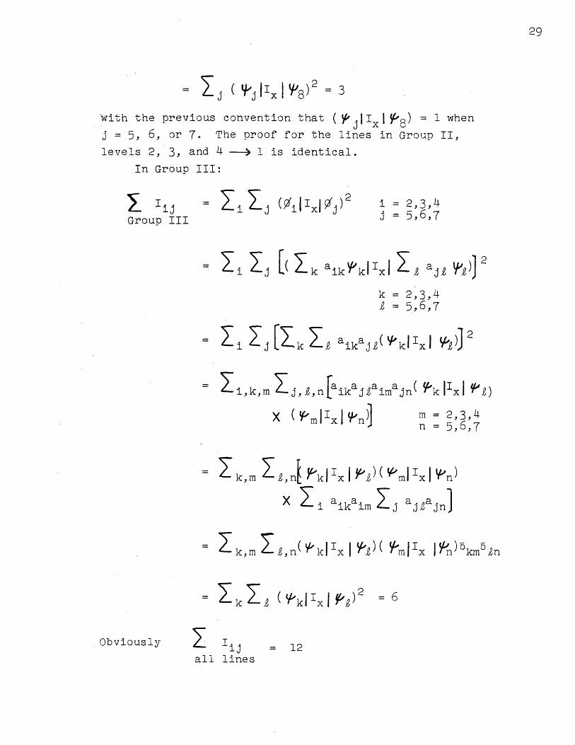
( •~xl • 2 = 3with the previous convention that (Vj IX 1&8) = 1 when
j = 5, 6, or 7. The proof for the lines in Group II,
levels 2, 3, and 4 -- 1 is identical.
In Group III:
I I ijGroup III
1 z-jz
-Ii ( k aik ikI
i = 2,3,4j = 5,6,7
Ix a,
=1i
I i,k,m
k = 2,3,42 = 5,6,7
[Zk Z aikaj( klxI V )J 2
zj, ,n aikajVaimajn( 'k Ix l)
m = 2,3,4n = 5,6,7
k, m
1 k,m
i,n Y''kjIx Ix £ ,m • Ix ' 'n)
X Ii aikaim z aj~ a n]
,n( k I x I ý) m( Ix I $n) km' n
( I'klIx I P')2 =6
Obviously
allIIijlines
= 12
Tj
9m( Im Ix I n I
30
The fact that the sums of the intensities of two sets
of lines must be one-fourth of the total intensity helps
greatly in assigning transitions to lines in a spectrum.
Up to this point it has been possible to assign the
lines into three multiplets. The assignment may be some-
what tentative if less than the theoretical number of
first order lines is observable because of degeneracy, if
some lines are very weak, or if there appear to be more
than four repeats of some line spacing.. The change from
A12( A13 to A12) A13 does not change the assignment of
the outer lines in the four line %ultiplet", so that if
all the Aij are assumed to be positive (the case in which
this is not true will be considered later) the line at
the lowest magnetic field in each four line group belongs
to Group I. The highest field ones are those in Group II.
Any assignment must meet the additional test that the
sums of the intensities of the lines in groups I and II
must have the proper values.
Because of the possibility of negative values of
Ai, the effect on the spectra of such changes in sign
should be investigated. With three Aij which can each
be either positive or negative, there are eight possibili-
ties, but four of these are related to the other four by
the reversal of all the signs. As is shown in Appendix A,
there is no way to distinguish between systems related by
reversal of the signs of all Aij; therefore, only four
possibilities need to be considered: one with all Aij
positive, and three with one negative.
In the first order spectrum of Figure 1, reversal of
the sign of an A.. interchanges the assignment of the
pairs of lines separated by that A.. In the figure,
changing to -IA12 1 will interchange assignments of lines
i and 2, 3 and 4, etc. In any spectrum for three spins,
the corresponding change occurs, and there will be four
possible ways to assign lines to transitions. These
31
alternate assignments should be considered to see what
effects they have upon the rules set up to test the
grouping of lines into four line multiplets.
The sum of the chemical shifts can still be deter-
mined because only the sum of the center positions of
each multiplet is needed. To use the intensity sums, the
assignment which corresponds to some A.. negative can be
set up (assuming the assignment into groups of four which
is for all A's positive has been found) by interchanging
the assignments of all pairs of lines whose separation
corresponds to the A.. which is to be negative. The3ij
new values for the appropriate transitions are then used
in the sums. In some cases which depart considerably
from first order, the intensity sums over groups I and
II will be three for only one or two of the four possible
assignments, allowing some to be eliminated. In a first
order spectrum, there exists no difference among the four
possible arrangements of the signs of the A...
In finding the sum of the Aij, the correct assignment
must also be used. If (v12 - V3 5 + v1 2 - v46 + v 1 3 - v 4 7 )
is chosen as the sum of the splittings in the assignment
corresponding to positive A's, then the same sum with new
values for the v's should be used in other assignments.
The algebraic sum of the A's results.
For there to be more than one assignment, other than
the four possibilities discussed so far, there must exist
a fortuitous relation among the parameters such that some
line spacings repeat more than four times. In this case
it is probable that the A.. are large, in which case theIj
intensities can probably determine the correct assignments.
If this fails, the only recourse is taking the spectrum
at another value of the magnetic field, H . If a set of
parameters can be found that predicts the spectrum at two
magnetic fields, it is extremely likely that-it is the
correct one, neglecting the possible existence of other
32
assignments differing only in the signs of the A's. It
should be added here that in the specific cases discussed
later, trying to use a set of parameters with a negative
A.. causes some small change in all parameters; however,
by far the major change is that the A has a different
sign.
After using the methods just described to determine
a correct assignment, there remains the problem of find-
ing the six parameters A1 2 , A1 3 , A23, v1 , 2, and v .
The method used here is that of assuming a set of para-
meters, calculating a spectrum on that basis, and adjust-
ing the parameters for the best fit, defined as the point
at which the differences between experimental and calculated
spectra are equal to or less than the estimated error in
the experimental spectrum. There remains a small range
for each of the parameters in which there is agreement
between calculated and experimental spectra. One comment
on this method is helpful: it is found that if in first
order a change in A12 , for instance, is indicated by
comparison of the experimental and calculated spectra,
then making a change in this direction improves the fit
between them. The choice of parameters is restricted by
the fact that the sums of chemical shifts and coupling
constants are known.
33
III. EXPERIMENTAL
Three systems of three spins, each of which has three
nonequivalent protons coupled to each other, were selected
for study. 2,4- and 2,5-dichloroaniline were studied in
solution, the three protons on the benzene ring being of
interest in both cases. The protons studied are completely
independent of the amine protons, which have a transition
in a different region of the spectrum. The 2,5-dichloro-
aniline (Eastman Kodak, White Label) was studied as a
saturated solution in carbon tetrachloride (reagent grade).
This solution was in the neighborhood of three molar, but
the exact concentration is not important because any
changes in the spectra with concentration are very small,
and because the same sample was used for all spectra.
To increase solubility, the 2,4-dichloroaniline (Eastman
Kodak, White Label) was dissolved in 80 ~6 carbon tetra-
chloride with 20 0/oacetone by volume. The total length
of the spectrum was about 3 cps. less (at 40 Mc.) than
when pure carbon tetrachloride was used, probably because
of a change in the chemical shifts. No explanation is
offered for this effect, although it could be a basis for
further work. The dependence of this effect upon the
concentration of the dichloroaniline is small, since
several samples made up at different times gave the same
spectra.
The third sample was styrene (Eastman Kodak, White
Label), the three vinyl protons being those of interest.
There is probably very little interaction between ring
protons and those on adjacent carbon atoms in side chains,
since no splitting of spectral lines attributable to a
coupling between these protons has been observed.
All samples were outgassed on a vacuum line by
freezing, pumping and melting several times, and sealed
into 5 mm. Pyrex tubes. This procedure is necessary for
L.
best resolution since the dissolved oxygen is paramagnetic
and, at concentrations resulting from equilibration with
the atmosphere, widens the lines noticeably by shortening
the spin-lattice relaxation times. The styrene was sub-
jected to a crude distillation while under vacuum, reducing
the concentration of the inhibitor to a level such that
the samples had to be used within several days to prevent
polymerization products and increased viscosity from
affecting the spectra.
All spectra were taken on a conventional Varian V4300B
High Resolution NMR spectrometer, operating at 10 and 40
megacycles. For the 22.55 Mc. work, a transmitter-receiver
following the Varian design was used. The standard 40 Mc.
Varian crossed coil probe was used in this case, but
with a different receiver coil, constructed so that it
resonated at the proper frequency with the capacity
included in the probe. It was not necessary to change
the tuning of the transmitter coil in the probe when
working at 22.55 Mc.
The spectra were recorded on the attached Sanborn
recorder, using only the center portion of the chart to
reduce nonlinearity to an acceptable level. At present
it is possible to measure line intensities more. accurately
than when these data were taken, and the use of a more
linear recorder is advisable. Also, it is recognized
now that in some cases accurate intensities are very impor-
tant. The error introduced by the recorder used here is
not considered to affect any of the results in an important
way, however.
The spectra were recorded as functions of time, as
is usual. Fortunately the method of changing magnetic
field is such that the deviation from a linear change of
field with time is so small as to be negligible. There
are some other factors which influence the magnetic field,
such as power line voltage and temperature of themagnet.
35
However, the changes in field introduced by these factors
do not preclude the assumption that the magnetic field
changes linearly with time.
The samples were in 5 mm. O.D. Pyrex tubes, so that
it was possible to spin them for best resolution (3, 8).
The procedure used to measure the line positions is
standard, but several precautions are necessary to reduce
error to a minimum. The spectra were taken at a sweep
rate (magnetic.field sweep) chosen to reduce the effects
of the several experimental err6rs. For rapid sweeps,
the line positions become uncertain and resolution decreases
because of transient effects. One particular transient
effect, "wiggles" (9), is especially disturbing where
several lines occur close together. Too large a sweep
rate, then, causes deterioration of the spectrum. If
the sweep rate is too slow the change of magnetic field
with time may not remain linear, since the changes in
magnetic field caused by other factors (such as temperature
changes) become relatively more important, Furthermore,
changes in magnetic field caused by variation in the
power line voltage occur mainly in small "steps" and the
longer the time spent in scanning a spectrum, the more
likely that one or more of these "steps" is to occur.
For measurement of positions it appears best to err (if
at all) toward the faster sweeps, since the uncertainty
in line positions increases more slowly there than in the
opposite case. For intensity measurement and for observa-
tion of small lines near larger ones, it is decidedly
better to reduce the transient distortion as much as
possible by employing a slow sweep.
Twelve or more spectra were taken at the chosen
sweep rate and the best of these spectra -- those showing
no obvious effects of change in magnetic field -- were
selected and the relative positions measured. Two prominent
lines at each end of the spectrum were used to establish

the 0 and 1000/0 points of a relative scale, and all the
other positions were measured relative to these points
by interpolation and extrapolation. The individual line
positions were averaged; this procedure is possible since
the positions are on a common basis. This average spectrum
can be used for calculation of parameters; however, the
parameters will differ from the true ones by a scale factor.
To determine this scale factor it is necessary to
measure the length of the selected interval (100%0/) in
the spectrum. This calibration is done by the standard
method of modulating the magnetic field 1o and observing
the side bands produced (38). For each line in the spectrum
there will be two or more side bands symmetrically disposed
around the line'. For suitable adjustment of the modulation
level and frequency, it is possible to observe three essenti-
ally identical spectra with the spacing between equivalent
points just AH = 2wVm where AH is the difference in
magnetic field of the two points, and vm the frequency of
the audio modulation. If one prefers, the spacing of the
spectra can be left in frequency units. From a recording
of the three spectra with a known audio modulation frequency,
the spacing between the lines selected as 0 and 100 0o can
be determined. Several such calibrations are averaged.
The frequency of the audio oscillator used for pro-
ducing the modulation was calibrated against a tuning
fork, the frequency of which had been measured to better
than 0.i /oby a frequency counter. The 60 cycle power
frequency was also used as a secondary standard. At
present it is known that this frequency is within 0.1
cps. of 60.0 cps., by direct measurement with a Hewlett-
Packard frequency counter.
The intensities can be measured from either the peak
height or the integrated area under the curve. Both
methods seem to give similar reproducibility. If, as
in the spectra taken here, there is no indication of
37
differing line widths, the peak height method is probably
better. This statement is true because field instability
is the mat important source of error and a change in mag-
netic field during the time a line is being traversed
will affect the width of the line, and hence the area,
but will not appreciably change the height. If the radio
frequency power level is too high for a given sweep rate,
there occurs the phenomenon known as saturation (9).
The main result is that the lines become broader, reducing
the resolution and modifying the intensities observed.
The complications introduced by this effect are avoided
by keeping the power level low, but still large enough
to maintain a proper signal-to-noise ratio. Finally, both
methods of intensity measurement are subjected to error
because of uncertainty in the positioning of the base line.
This uncertainty occurs most commonly when the lines are
not all completely resolved.
The intensities from each spectrum are normalized so
that the total intensity is twelve. This number is used
because it is that which appears in a calculated spectrum
if the definitions given in Section II are used. The
intensities of a set of spectra may now be averaged, since
they are on a common basis.
38
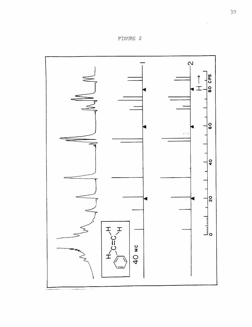
IV. RESULTS AND DISCUSSION
In Figures 2, 4, 5, 7, and 8 are shown typical spectra
of the three compounds studied. These of course are
individual spectra, and their line positions and intensities
are not in all cases identical to the average of these
quantities used in the analysis. Shown with the spectra
are ones calculated using parameters which result in the
best fit between the calculated and average experimental
spectra at 40 Mc. This determination is discussed in
more detail later. The results for the three compounds
will be given individually.
Styrene
The upper trace in Figure 2 shows the spectrum of
styrene at 40 Mc. Eleven of the first order lines of the
vinyl protons are obvious toward the right. The large
line on the left and several small satellites on each
side are from the five ring protons. The twelfth line
of the vinyl group is somewhat obscured by the satellites
on the large line. In addition, there is a small combina-
tion line which is observable at a larger amplification.
Its position is at about 37 cps. on the scale and agrees
with that given in the calculated spectra. Below the
experimental trace are twn ca~lculaRted spectra based upon
two possible assignments of transitions to line frequencies.
The two given here match the average experimental one to
within experimental error. (In Figure 3 are given two
other assignments which do not fit the experimental
intensities, but do fit the line positions.) The chemical
shifts are designated by the solid triangles; these are
the positions where the resonances for the three protons
would occur if there were no spin-spin coupling. It is
seen that these positions are not exactly in the centers
i
FIGTUE 2
C\j
0(0
4
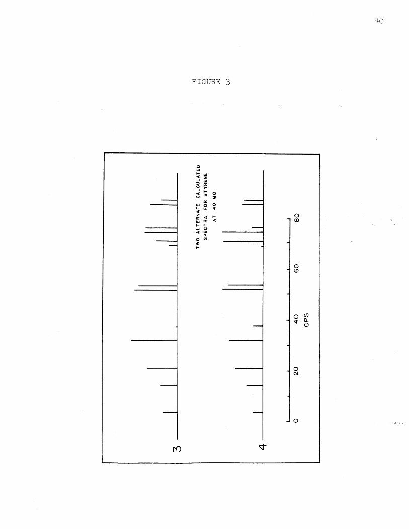
FIGURE 3
ra
i
i
a.
Bi
ji
r
I
t
r
i
0
0(D
O
O
c(i
L
wt- w
o W
('JO 0
Jo -3
4Ww06
IX
I•
NO ;I
of the groups of four lines; this fact indicates departure
from a first order spectrum.
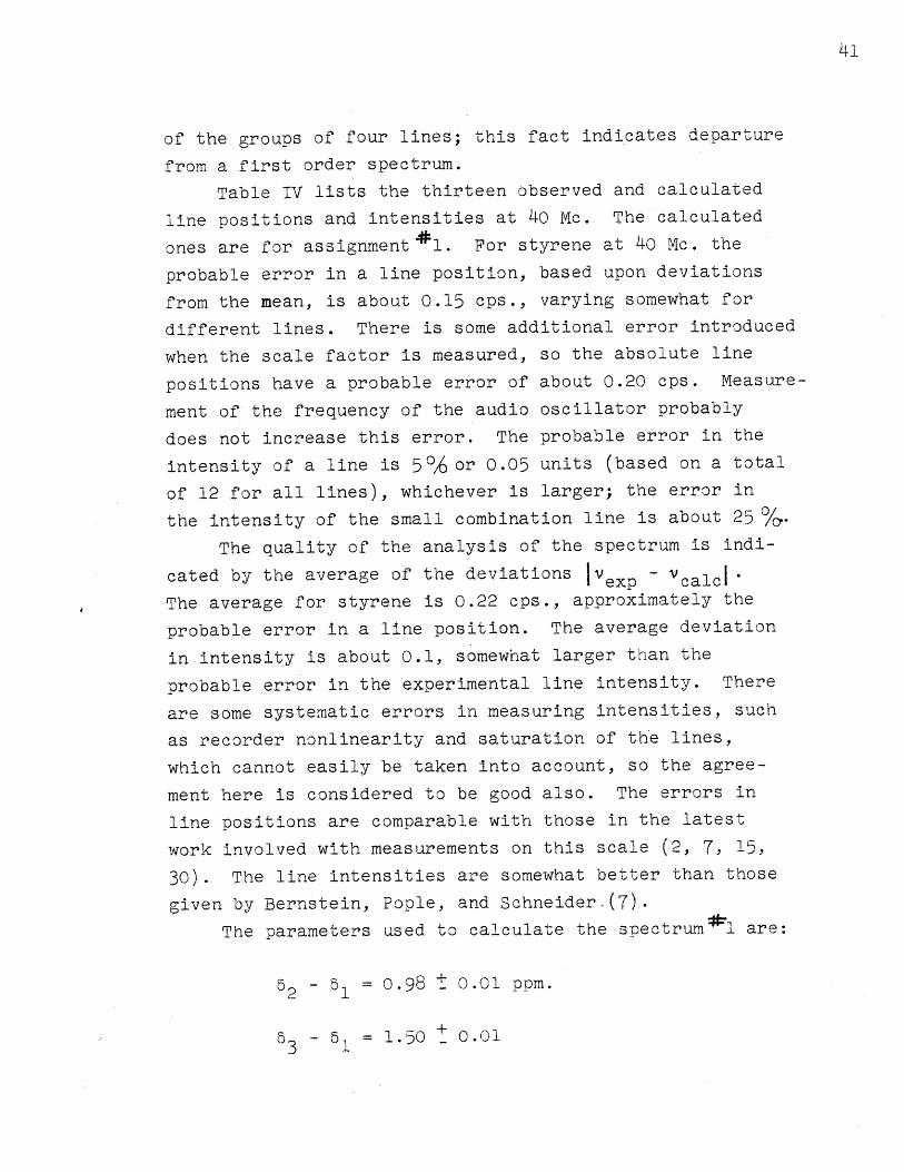
Table IV lists the thirteen observed and calculated
line positions and intensities at 40 Mc. The calculated
ones are for assignment 1. For styrene at 40 Mc. the
probable error in a line position, based upon deviations
from the mean, is about 0.15 cps., varying somewhat for
different lines. There is some additional error introduced
when the scale factor is measured, so the absolute line
positions have a probable error of about 0.20 cps. Measure-
ment of the frequency of the audio oscillator probably
does not increase this error. The probable error in the
intensity of a line is 5 0 6 or 0.05 units (based on a total
of 12 for all lines), whichever is larger; the error in
the intensity of the small combination line is about 25 /.
The quality of the analysis of the spectrum is indi-
cated by the average of the deviations IVexp - VcalcI•
The average for styrene is 0.22 cps., approximately the
probable error in a line position. The average deviation
in intensity is about 0.1, somewhat larger than the
probable error in the experimental line intensity. There
are some systematic errors in measuring intensities, such
as recorder nonlinearity and saturation of the lines,
which cannot easily be taken into account, so the agree-
ment here is considered to be good also. The errors in
line positions are comparable with those in the latest
work involved with measurements on this scale (2, 7, 15,
30). The line intensities are somewhat better than those
given by Bernstein, Pople, and Schneider (7).
The parameters used to calculate the spectrum 1l are:
5- 2 1 = 0.98 + 0.01 ppm.
5 5 = 1.50 _ 0.013 1
42
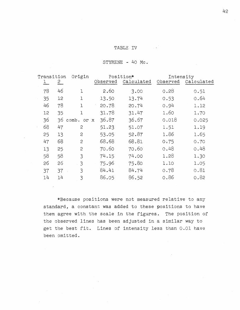
TABLE IV
STYRENE - 40 Mc.
Transition1 2
78 4635 1246 7812 35
Origin
1
1
1
1
36 36 comb. or x
68 4725 1347 68
13 25
58 5826 26
37 3714 14
2
2
2
2
3333
Position*Observed
2.60
13.5020.78
31.78
36.87
51.23
53.05
68.68
70.60
74.15
75.9684.41
86.05
Calculated Obse
3.00
13.7420.74
31.47
36.67
51.0752.87
68.81
70.60
74.00
75.8084.74
86.52
Intensity.rved Calculated
0.28
0.53
0.941.600.o18
1.511.86
0- 750.481.281.10
0.780.86
0.510.64
1.12
1.70
0.025
1.19
1.65
0.70o.48
1.30
1.05
0.810.82
*Because positions were not measured relative to any
standard, a constant was added to these positions to have
them agree with the scale in the figures. The position of
the observed lines has been adjusted in a similar way to
get the best fit. Lines of intensity less than 0.01 have
been omitted.
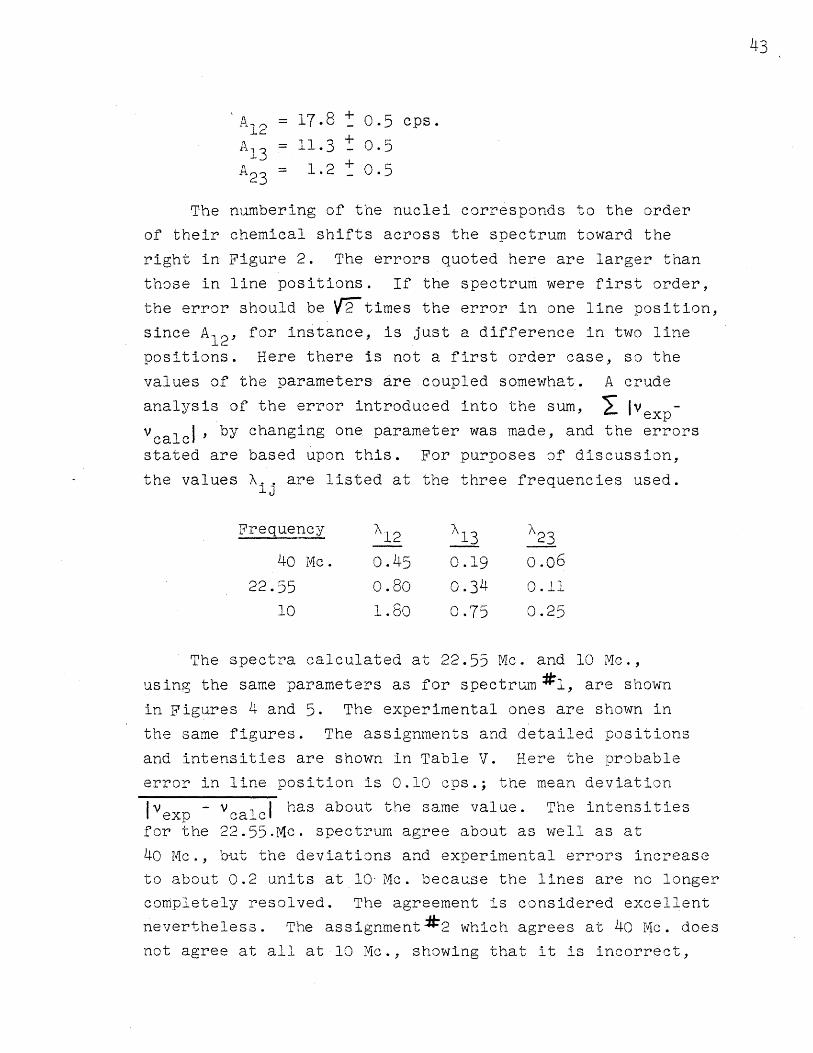
A2 = 17.8 + 0.5 cps.A13 = 11.3 + 0.5A23 = 1.2 + 0.5
The numbering of the nuclei corresponds to the order
of their chemical shifts across the spectrum toward the
right in Figure 2. The errors quoted here are larger than
those in line positions. If the spectrum were first order,
the error should be V-times the error in one line position,
since A12 , for instance, is just a difference in two line
positions. Here there is not a first order case, so the
values of the parameters are coupled somewhat. A crude
analysis of the error introduced into the sum, T Ivex p
VcalcI, by changing one parameter was made, and the errors
stated are based upon this. For purposes of discussion,
the values A.. are listed at the three frequencies used.13
Frequency l2 13 23
40 Mc. 0.45 0.19 0.06
22.55 0.80 0.34 0.11
10 1.80 0.75 0.25
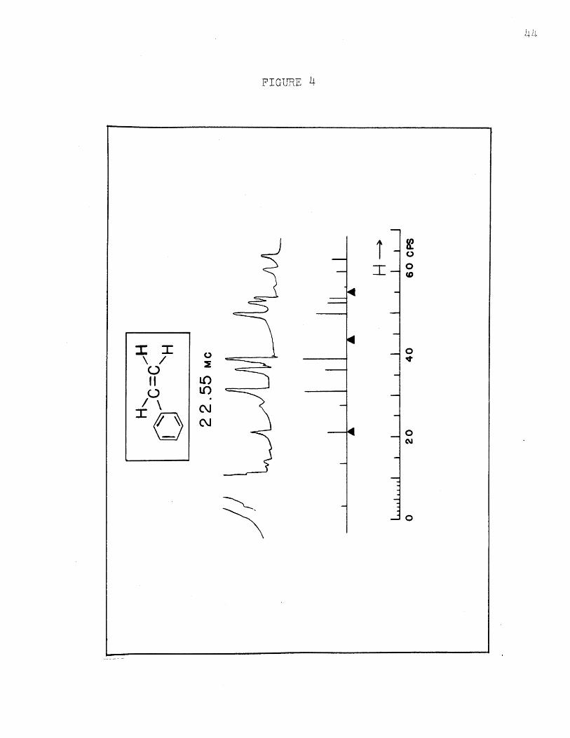
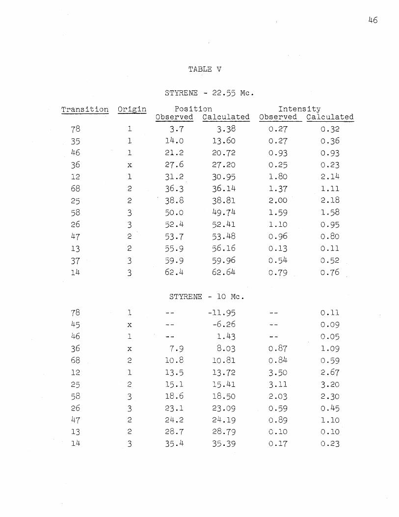
The spectra calculated at 22.55 Mc. and 10 Mc.,
using the same parameters as for spectrum :I, are shown
in Figures 4 and 5. The experimental ones are shown in
the same figures. The assignments and detailed positions
and intensities are shown in Table V. Here the probable
error in line position is 0.10 cos.; the mean deviation
IVexp - VcalcI has about the same value. The intensities
for the 22.55.Mc. spectrum agree about as well as at
40 Mc., but the deviations and experimental errors increase
to about 0.2 units at 10 Mc. because the lines are no longer
completely resolved. The agreement is considered excellent
nevertheless. The assignment*2 which agrees at 40 Mc. does
not agree at all at 10 Mc., showing that it is incorrect,
FT GTRE M 4
I -
4
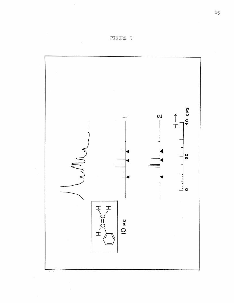
FIGURE 5
o
0
NJ
(L)I.
0r
II
, a
Transition Ori0in
78
3546
36
12
6825
5826
47
133714
TABLE V
STYRENE - 22.55 Mc.
PositionObserved Calculated
3.7 3.3814.0 13.60
21.2 20.72
27.6 27.20
31.2 30.95
36.3 36.14
38.8 38.81
50.0 49.74
52.4 52.41
53.7 53.4855.9 56.1659.9 59.9662.4 62.64
IntensityObserved Calculated
0.27 0.32
0.27 0.36
0.93 0.93
0.25 0.23
1.80 2.14
1.37 1.11
2.00 2.18
1.59 1.58
1.10 0.95
o.96 0.80
0.13 0.110.54 0.52
0.79 0.76
STYRENE - 10 Mc.
7.910.8
13.515.1
18.6
23.1
24.2
28.7
35.4
-11.95-6.26
1.43
8.0310.81
13.7215.41
18.5o23.09
24.19
28.79,
35.39
78
4546
366812
25
5826
47
1314
0.11
0.09
0.051.09
0.592.67
3.202.30
0.451.10
0.10
0.23
0.87
0.84
3.50
3.112.03
0.590.89
c.100.17
47
and illustrating the value of having data corresponding to
more than one value of the magnetic field.
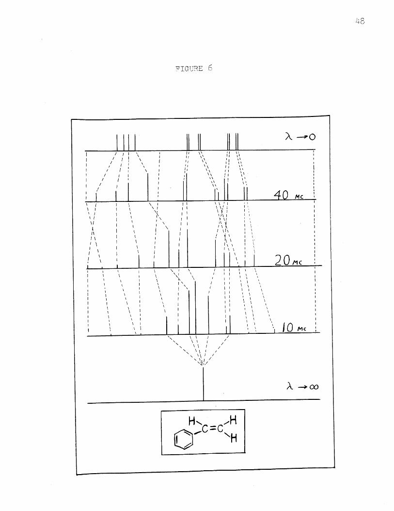
The assignment of transitions to lines at 40 Mc. is
given with the line frequencies in Table IV. Figure 6 then
correlates the lines observed at several frequencies and
shows the relationship of the spectra. It also shows which
lines remain with nonzero intensity in the limit of no
chemical shift. The line which corresponds to the transi-
tion v36 , the one observable combination line at 40 Me.,
is seen to be one of the five largest lines at 10 Me. It
has intensity 1.00 in the limit of no chemical shift.
Assignment l corresponds to all Aij positive. The
assignment- 2, which also fits closely at 40 Mc., is also
given in the table. This new assignment has interchanged
all labeling of lines separated by the splitting correspond-
ing to A1 2. Now, there is a negative value for AI2 and
the parameters are:
6 - 51 = 0.99 ppm.
63 - 61 = 1.51
A12 -17.8 cps.
A 3 11.3
A23 = 1.4
As was mentioned earlier, this set is incorrect since it
does not at all agree with experiment at 10 Mc.
It is interesting to note what occurred in changing
from AI2>0 to Al2 <0. The changes made in the other para-
meters are small, but are necessary to get the best fit of
the line positions. The assignments 3 and 4 are based
upon sets of parameters with A13 40 and A2 3 (0. These two
can be rejected even at 40 Mc. That all assignments correspond-
ing to some A.. negative have been eliminated has shown that-Jthe relative signs of the three coupling constants must be
the same. There is no other assignment with different mag-
IGURiTE 6
X - 0
I \
I I
S- co
I I I I II II
/ ~I/
/
'I' I'I
I'
I'
I
II II
I
r 49
hydrogens, are vl' = 25, v2 ' = 65, and v3 ' = 85 cps.
Using as model compounds a-methyl styrene and trans-0-
methyl styrene (prepared by C. Bumgardner), numbers 1,
2, and 3 can be assigned to particular protons in the vinyl
group. In a-methyl styrene the protons have chemical
shifts of about 72 and 86 cps., relative to the ring.
If it is assumed that the ring differs by only a small
amount between these compounds, which is certainly correct
to the degree of accuracy needed here, then the *1 proton
is evidently the a one in styrene. Therefore, the unusual
chemical shift of this proton is probably connected with
the well known ability of the ring to conjugate with the
a• position.
In trans-P-methyl styrene the spectrum is complicated
by coupling of the methyl protons to one ethylenic proton.
No complete analysis has been made, but there appears to
be a coupling between the two vinyl hydrogens of 17 + 1 cps.
It would appear that the 17.8 cps. coupling in styrene is
that between trans hydrogens. This is in accord with the
observation that in several compounds, the coupling between
HH and F19 is larger if they are trans, instead of cis,
on a double bond (25). The assignment then is:
nitudes of v's and A's possible at 40 Mc., because there
is no other with the proper repeated spacings.
In Appendix B are given some details pertaining to
the calculation of the spectrum at 22.55 Mc. It demon-
strates vividly the effects of the spin-spin couplings in
mixing the zero order wave functions.
The values of the parameters calculated from the
spectrum of styrene are rather unusual. Proton 1 is
far removed from the position usually associated with
ethylenic hydrogens (37). Also A2 3 is extremely small.
These values should be examined more closely. The chemical
n~ · ~r Tr~ r\ 17u ~or~ ur· iu Ir Ir ri
a
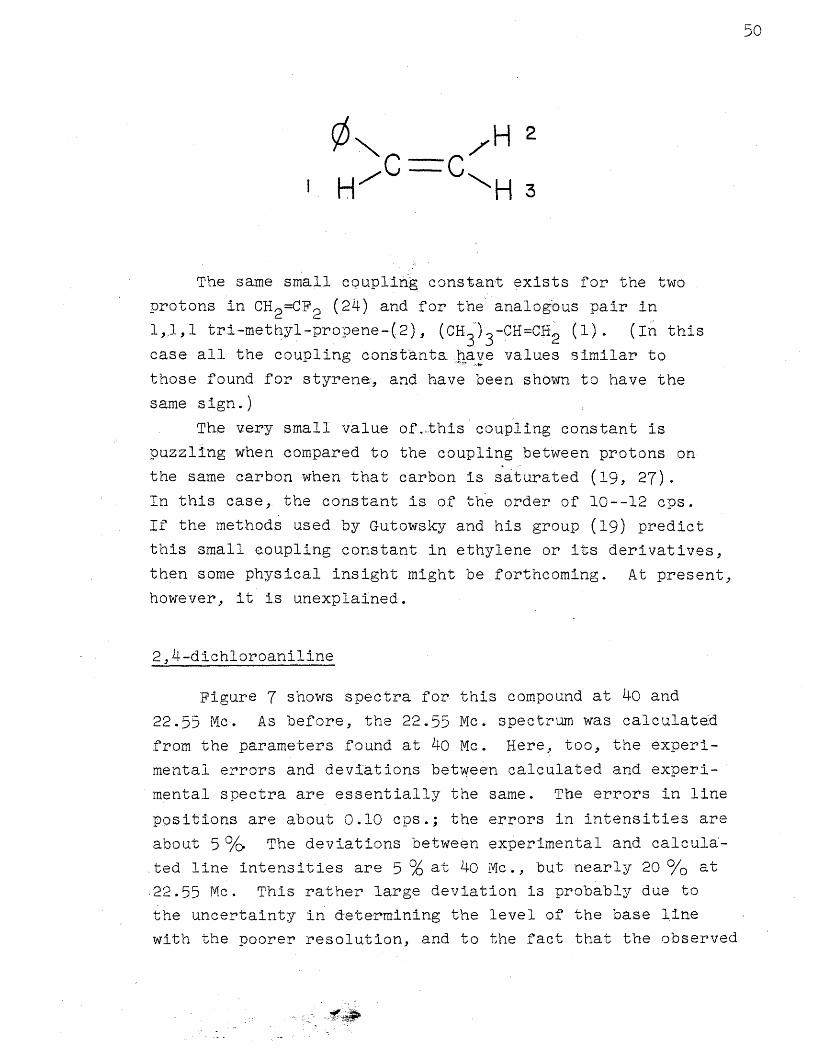
C -C
The same small coupling constant exists for the two
protons in CH2=CF 2 (24) and for the analogous pair in
1,1,1 tri-methyl-propene-(2), (CH3 )3 -CH=CH 2 (I). (In this
case all the coupling constants..have values similar to
those found for styrene, and have been shown to have the
same sign.)
The very small value of.this coupling constant is
puzzling when compared to the coupling between protons on
the same carbon when that carbon is saturated (19, 27).
In this case, the constant is of the order of 10--12 cps.
If the methods used by Gutowsky and his group (19) predict
this small coupling constant in ethylene or its derivatives,
then some physical insight might be forthcoming. At present,
however, it is unexplained.
2, -dichloroaniline
Figure 7 shows spectra for this compound at 40 and
22.55 Mc. As before, the 22.55 Mc. spectrum was calculate:d
from the parameters found at 40 Mc. Here, too, the experi-
mental errors and deviations between calculated and experi-
mental spectra are essentially the same. The errors in line
positions are about 0.10 cps.; the errors in intensities are
about 50/. The deviations between experimental and calcula'-
ted line intensities are 5 0 at 40 Mc., but nearly 20 o/o at
.22.55 Mc. This rather large deviation is probably due to
the uncertainty in determining the level of the base line
with the poorer resolution, and to the fact that the observed
L-

f IGTr•E 7
o
I I:
U
0
I -o
LOLO
0N
0
rO"N
rr)
52
lines are the approximate superposition of several, and
the heights may not be additive.
The solid triangles again give the chemical shifts.
The proton numbering is 1, 2, 3 toward the right. Table
VI gives the assignment, and calculated and observed positions
and intensities. At 40 Mc. all first order lines are
observed. In addition, it should be pointed out that the
small line in the upper spectrum, at about 17 on the scale,
is a combination line. Table VI shows that in the 22.55
Mc. spectrum there are two combination lines, although
they occur in conjunction with other first order lines.
In the latter spectrum, one first order line is not experi-
mentally observable.
The parameters which give the best fit at 40 Mc. are:
E5 2- 5• = 0.230 t 0.007 ppm.
5 - 1 = 0.570 1 0.007
A1 2 = 2.4 k 0.4 cps.
A 3 =0.4 0.3
A2 3 =8.8 0o.4
No assignments were tried for any Ai. negative because-Jlines such as those for transitions 78 and 35 are not at
all completely resolved. These pairs would have to be
separated to use any of the tests which are useful for
rejecting incorrect assignments, such as those involving
the intensities of certain groups of lines. Because
there is good agreement at the two frequencies, it is
highly probable that the set of parameters is the correct
one, neglecting the possibility of others with different
signs of the A's.
The splitting of the pairs 78 and 35, 46 and 12, 58
and 37, and 26 and 14 is about 0.6 cps. in the experimental
spectrum. If A3 = 0 is used in the calculation, thereremains a residual splitting at 3
remains a residual splitting at 40 Mc. of about 0.4 cps.
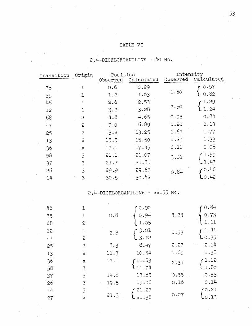
TABLE VI
2, 4-DICHLOROANILINNE
Transition Origin
1783546
6847.25
13
36583726
PositionObserved
o.61.2
2.6
3.2
7.0
13.215.5
17.121.1
21.729 -9
30.5
Calculated
0.29
1.03
2.53
3.28
4.656.89
13.2515.50
17.45
21.07
21.8129.67
30.42
IntensityObserved Calculated
1.50
2.50
0.95
0.20
1.67
1.27
0.11
3.01
0.84
0.570.82
1.291.240.84
0.13
1.77
1.33
0.o081.591.43
o0.46o.42
2,4-DICHLOROANILINE
0.8
2.8
8.310.312.1
14.0
19.5
21.3
S0.900.94%1.05
( 3.01..3.12
8.4710.5411.63
S11.7413.8519.o6
21.2738021.38
- 22.55 Mc.
3.23
1.53
2.27
1.69
2.31
0.550.16
0.27
- 40 Mc.
3568
13
36583726
14
27
0.84
0.731.11
1.41
0.35
1.38
1.12
1.800.53
0.14
0.13
If A!3 = .4 cps. is included, then the splitting is .75 cps.,
approximately the observed splitting. This splitting is
not accurately known so the A,3 is subject to some error.
To decide which of the chemical shifts corresponds
to which of the hydrogens in the molecule, it is necessary
to extimate what the values for Ao, Am, and A are. (A0
means the coupling constant between two protons ortho to
one another on a benzene ring, etc.). McConnell (22) cal-
culates that the contribution to the coupling constant by
the ) electron system of a ring is of the order of 1 cps.
or less for all pairs of protons. Therefore, the coupling
constants should behave as in most other compounds and
decrease with increased separation of the hydrogens.
Gutowsky (15) makes this assumption and finds that for
several systems studied A ° 8, Am -2.5, and A (1. If
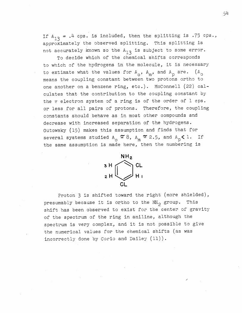
the same assumption is made here, then the numbering is
NH2
aH CL
2H HCL
Proton 3 is shifted toward the right (more shielded),
presumably because it is ortho to the NH2 group. This
shift has been observed to exist for the center of gravity
of the spectrum of the ring in aniline, although the
spectrum is very complex, and it is not possible to give
the numerical values for the chemical shifts (as was
incorrectly done by Corio and Dailey (11)).
55
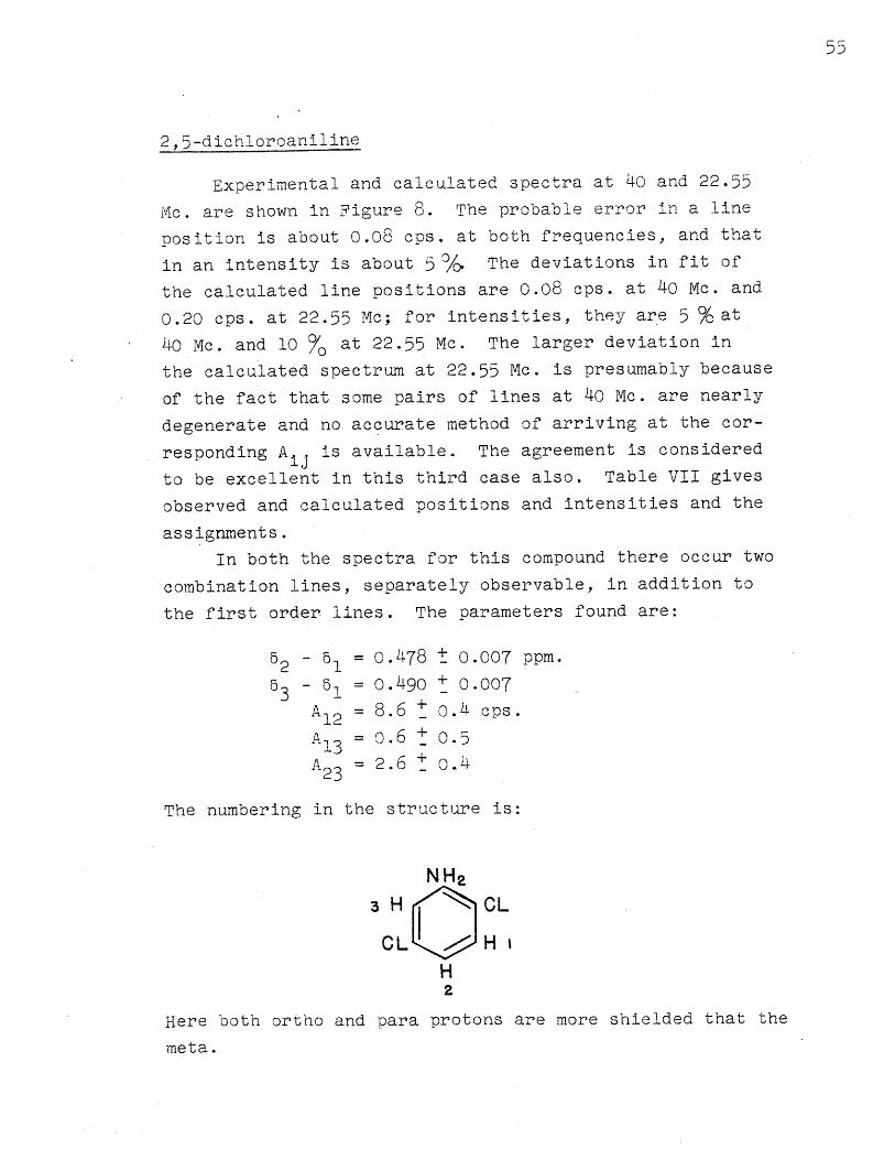
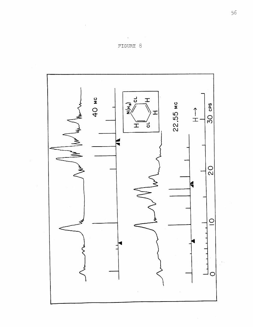
2,5-dichloroaniline
Experimental and calculated spectra at 40 and 22.55
Mc. are shown in Figure 8. The probable error in a line
position is about 0.08 cps. at both frequencies, and that
in an intensity is about 5%/0 The deviations in fit of
the calculated line positions are 0.08 cps. at 40 Mc. and
0.20 cps. at 22.55 Mc; for intensities, they are 5 % at40 Mc. and 10 0/ at 22.55 Mc. The larger deviation in
the calculated spectrum at 22.55 Mc. is presumably because
of the fact that some pairs of lines at 40 Mc. are nearly
degenerate and no accurate method of arriving at the cor-
responding Aij is available. The agreement is considered
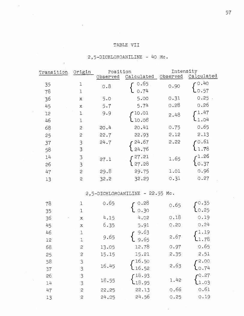
to be excellent in this third case also. Table VII gives
observed and calculated positions and intensities and the
assignments.
In both the spectra for this compound there occur two
combination lines, separately observable, in addition to
the first order lines. The parameters found are:
52 - 51 = 0.478 t 0.007 ppm.53 - 1 0.490 + 0.007
A1 2 = 8.6 + 0.4 cps.
A, = 0.6 + 0.513A23 = 2.6 0.4
The numbering in the structure is:
NH2
H CL
CLK HIH2
Here both ortho and para protons are more shielded that the
meta.
3'TGTJE. 8
k
B;
Ii
i
57
TABLE VII
2,5-DICHLOROANILINE - 40 Mc.
Transition Origin
3578364512
466825
375814
26
47
PositionObserved
0.8
5.0
5.79.9
20.4
22.7
24.7
27.1
29.8
32.2
IntensityCalculated Observed
o 0.65S0.74
5.005.74
10.01o10.08
20.41
22.93
( 24.6724.7627.2127.2829.75
32.29
0.90
0.31
0.28
2.48
0.752.12
2.22
1.65
1.01
0.31
Calculated
o.400.57
0.250.26
(1.47l.o4
0.652.13
o.61
(1.781.26
0.370.960.27
2,5-DICHLOROANILINE - 22.55 Mc.
0.280.304.02
5.91{ 9.639.65
12.78
15.21S16.5016.52
(18.9318.95
22.13
24.56
0.65
0.180.20
2.67
0.97
2.35
2.63
1.42
0.66
0.350o.250.19
0.24
1.19S1.780.652.51
2.000.74
0.27(.103
o.61
0.25 0.19
783536454612
68
0.65
4.15
6.35
9.65
13.0515.15
16.45
18.55
22.25
24.25
47
13
It is curious to note that here if one takes A13 = 0,
the residual splitting "corresponding" to A13 is 0.4 cps.,
but that introducing A 3 = .4 reduces the splitting,
contrary to what happened in the case of 2,4-dichloroaniline.
This agrees with experiment in that with the existing
resolution there is no splitting of the appropriate lines.
The difference in the two cases is connected in detail with
the special values of the parameters.
This case also demonstrates that the values of rijbetween pairs of nuclei do not individually determine the
mixing of the wave functions and therefore the departure
from a first order spectrum. The value of \23 is 6.5 at
40 Mc. However because there is a great difference between
A12 and A13 , the effects, such as the disappearance of some
lines for protons 2 and 3, which occur when A12 = Al3, do
not appear. This is explained qualitatively by saying that
the inequality of A12 and Al3 disturbs the coupling of
protons 2 and 3 -- which would exist if A 12 = A1 3 -- into
singlet and triplet states (uncouples them). It is worth-
while to point this out since, although most workers in
the field undoubtedly recognize this phenomenon and at
least one illustration has appeared in print (5), it is
foreign to the usual first order theory which is often
applied in preliminary discussions of spectra.
P
59
V. CONCLUSION
Although it is possible that there will be essential
deviations between experimental and calculated spectra
when it becomes possible to measure the experimental
spectra more accurately, the present work indicates that
even for systems which depart greatly from first order
behavior there is a unique set of parameters which can
describe the system over a range of magnetic fields in
accord with equation 1. For styrene at 10 Mc., for instance,
the values of hij are 1.8, .75, and .25, indicating a
great departure from first order behavior. Here the agree-
ment between calculated and experimental spectra is excellent,
indicating that there is indeed a set of parameters which
describes the system at this field. Lest this seem to be
a fatuous statement, it should be remarked again that no
test of the spin Hamiltonian to this accuracy has heretofore
been given. In addition, this is the same set which was
determined at a much higher field (appropriate to 40 Mc.).
Indirectly then, it shows that the v ' vary linearly with
the magnetic field and that the Aij are independent of
field.
Consideration of the spectra given at the lower frequen-
cies indicates that interpretation of these spectra is
very difficult. If no aids, such as those shown in
Section II involving the form of the spectrum, were known,
it is highly likely that it would be impossible to get a
trial starting set of parameters, The correlation diagram
for styrene, Figure 6, helps to illustrate this difficulty.
It is easy to group the lines at 40 Mc. into three groups,
one for each nucleus. Although the proper groupings at
10 Me. can be seen in the diagram, it would be exceedingly
difficult to reproduce them from an experimental spectrum.
60
The method given by McConnell and Anderson (23) for
determining some of the parameters from experimental first,
second, and higher moments of the spectrum does not change
the above statements very much. The higher moments (fourth
and above) which are necessary to determine the coupling
constants are always very inaccurately known because of
experimental errors. It was found, in collaboration with
Dr.. D.M. Graham, that for 2,4-dichloroaniline at 40 Mc.
an:. intelligent guess was as close to the correct parameters
as the results of the method of moments. The moment method
is nonetheless useful in determining a set of approximate
parameters in the cases with greater mixing.
The present work is the first in which combination
lines have been observed experimentally. Many of the papers
dealing with the analysis of spectra (7, 15, 30) seem to
convey the general feeling that combination lines are always
weak. The correlation diagram shows that this is not the
case, and that at low fields one combination line, the one
which appears in the spectrum even at 40 Mc., grows to
unit intensity. At 10 Mc., for instance, it is much
larger than all but four first order lines. The fact that
the sane eight energy levels which describe the first order
lines also give the correct positions for the observable
combination lines is further proof that the methods used
for describing the spectra are correct.
Finally, the example .of styrene shows that at least
in favorable cases the relative signs of the coupling
constants can be determined unambiguously. The methods
given here can also determine the correct signs without
a complete analysis. The one case in which the signs
were determined showed that the coupling constants were
all of the same sign, in accord with theory (16, 21, 33).
I
61
VI. INTRODUCTION: INTERNAL ROTATION
Several workers have observed that the high resolution
nuclear resonance spectra of certain ethane-like substances
contain more lines than can be explained by assuming com-
pletely free rotation about the carbon-carbon bond (14, 27,
30). In addition, a strong temperature dependence has
been observed for the chemical shift in one compound (12).
This dependence was originally ascribed to changing ampli-
tudes of torsional oscillation of a particular isolated
rotational isomer. The correct explanation for all these
observations appears to be that internal rotation, even
when rapid, may give rise to unequivalences among nuclei
when some internal configurations are energetically more
favorable than others. In addition, the temperature
dependence of a spin-spin splitting between a pair of lines,
which must exist if this explanation is correct, has been
demonstrated by Graham and Waugh (14).
It is extremely desirable that such cases be examined
further to substantiate the theory, and to connect in
detail the temperature dependence with the energetics of
the internal rotation. This connection must exist, but
in the cases studied so far its quantitative elucidation
has been difficult. Such a quantitative connection would
be of great value because it would provide a new means
of measuring the energy differences between rotational
isomers, and thereby shed light on the general problem of
internal rotation, in which considerable theoretical
interest already exists (26).
62
VII. THEORY OF ROTATIONAL AVERAGING
The usual description of the potential energy of a
substituted ethane as a function of the azimuthal angle paround the carbon-carbon axis, is one with potential minima
when the substituents are separated by approximately 600
(staggered) and maxima when they are separated by 00
(eclipsed). If the further assumption is made that the
height of the maxima is several times the differences
between minima, there will be two extremes which are of
interest. In one case the barrier is high enough compared
to kT so that the lifetime of the molecule in one configura-
1tion is long compared with where 5w is a chemical
shift or spin-spin coupling. In this case any fine structure
resulting from 6w is observableofor each of the several
configurations which may be present. If the lifetimes are
1short with respect to then a time-averaged Hamiltonian
should be used to describe the system. For the substances
of interest here, the latter case is appropriate at room
temperature since the spectra observed are attributable
to a single molecular species and not to superposition of
several spectra. In addition, some instances have been
reported in which, by going to lower temperatures (-800 C.),
it was possible to increase the lifetimes enough so that
spectra of the several distinct isomers appeared (27, 28).
The fact that this time averaging is necessary was recog-
nized independently by Nair and Roberts (27), Shoolery
and Crawford (36), Graham and Waugh (14), Gutowsky et al.(15),
and Pople (29). Two cases where it was appropriate but
was not recognized, have also appeared (12, 20).
The simplest possible model which contains all of the
necessary features is the following: the lifetimes of the
63
rotational isomers are short and the time average state of
a molecule is just a superposition of the three staggered
isomers taken in proportion to single Boltzman factors for
these states. In saying this it is assumed that the time
spent in transitions between states is small and that each
isomer occupies no more than one torsional oscillation
level.
There are two classes of compounds with different
symmetries which Shoolery and Crawford discuss (36); how-
ever, it is convenient to break down one of these further.
Class I includes molecules of the sort CX2R-CR'R"Y,
where X and Y may or may not be the same, and R, R', and
R" do not have magnetic nuclei which interact with X and
Y. Here the two nuclei X can have different chemical
shifts and coupling constants to Y, as will be seen later.
Class IIA includes molecules such as CX2RCY 2R', in which
there can be no chemical shift between the two X nuclei
or between the two Y nuclei because, given one gauche
isomer in which the X's (or Y's) have different chemical
shifts, there is another isomer of equal energy, hence
probability, in which the X's are simply interchanged.
These two must average to give no chemical shift. In this
case, however, there can be two values of AXY , indicating
a nonequivalence of the X's and Y's. The spectrum will
show this nonequivalence in that, instead of a triplet of
intensity 1:2:1 for X or Y, the center line is split into
four components. (The lines usually occur in pairs, how-
ever). Shoolery and Crawford (36) and Graham and Waugh (14)
observed this splitting in several cases.
Class IIB includes molecules such as CXR 2CR'Y 2, inwhich the spectrum shows no effects of nonequivalence,
but the parameters involved can change with temperature
as do those in the other cases.
I
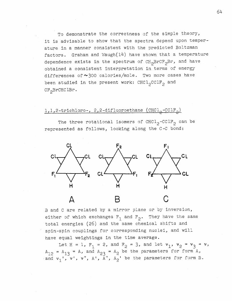
64
To demonstrate the correctness of the simple theory,
it is advisable to show that the spectra depend upon temper-
ature in a manner consistent with the predicted Boltzman
factors. Graham and Waugh(14) have shown that a temperature
dependence exists in the spectrum of CH2BrCF 2Br, and haveA A 4 -ri r\'= ='cn ni4tr V-in ite- n tati n f ; ner y
differences of~300 calories/mole. Two more cases have
been studied in the present work: CHC1 2CC1F 2 and
CF2BrCHC1Br.
1,1,2-trichloro-, 2,2-difluoroethane (CHCl~-CC1FD)
The three rotational isomers of CHCl 2-CClF2 can be
represented as follows, looking along the C-C bond:
F2 FI
C
F CL F7 1
H L.
CL
CL
A B CB and C are related by a mirror plane or by inversion,
either of which exchanges F1 and F2. They have the same
total energies (26) and the same chemical shifts and
spin-spin couplings for corresponding nuclei, and will
have equal weightings in the time average.
Let H 1, F1 = 2, and F2 = 3, and let v1, 2 = 3 = ,
A12 A1 3 = A, and A23 = A2 be the parameters for form A,
and v,', v', v", A', A", A2 ' be the parameters for form B.
Iri ~ r; Iir
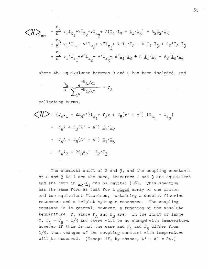
65
<1Žme A n 1 z2+vI z3 A(IlI 2 + 1113) + A2 12 I 3
no+n B I .+ V'I z+ v"I + A'I 1 2 + A" 1. 3 + A 2'I13n- 1'zl z z3+ 1 + .1 3 + A2 i2
+ CV I +v"I + v'I + A"I *I + A'I -I + A'in n z1 2 z 3 1 2 13 2 12
where the equivalence between B and C has been included, and
nA e - A/ ikTn e-E i/kT A
collecting terms,
<j >= (fA 1 + 2fBv')Itz + fAV + fB(VI + V) (I z + ! z211 2
+ fAA + fB(A' + A") 'II2
+ fAA + fB(A' + A") 1.13
+ f AA2 + 2fBA 2 1213
The chemical shift of 2 and 3, and the coupling constants
of 2 and 3 to 1 are the same, therefore 2 and 3 are equivalent
and the term in 12 -3 can be omitted (16). This spectrum
has the same form as that for a rigid array of one proton
and two equivalent fluorines, containing a doublet fluorine
resonance and a triplet hydrogen resonance. The coupling
constant is in general, however, a function of the absolute
temperature, T, since fA and fB are. In the limit of large
T, fA = fB = 1/3 and there will be no changs with temperature,
however if this is not the case and fA and fB differ from
1/3, then changes of the coupling constant with temperature
will be observed. (Except if, by chance, A' + A" = 2A.)
L
66
The chemical shifts of H and F presumably vary with tempera-
ture also, but an external reference and an accurate method
of measurement would be necessary to verify this. For this
work the spin coupling can be measured more accurately in
any case, so it alone has been studied.
The relation for the H-F spin-spin coupling is
Aobs = fAA + f (A' + A " )
EB • - EAwhere if = X,RT
f -X -Xthen - e = f e - and fA + 2f= 1
S-P P "P -X f 1 . -X-X I e~~f L5 1_ __
A A 1 + 2 e 1 + 2e -
Then if A' + A" _- 2A + 2g, Aobs = fAA + f(2A + 2g)
= A + 2gf•
So the change in Aobs is proportional to fB if g is a
constant. The value of g will be constant if there are
no changes in the values A, A', and A" with temperature.
Such changes could be produced by changes in population
of torsional oscillation states, by modification of the
wave functions, by changes in population of vibrational
states, and by changes in intermolecular interactions.
It will be assumed that these changes are of a smaller
order than the one produced by changing rotational
averaging, since they have never been observed.
A plot of Aobs against ff for different values ofE -E A pB A , which connects X and 1 , should give a straight
li&e for the proper value of B- A A more complete
analysis is not possible because there is at present no
way of predicting what values A, A', and A" should have.
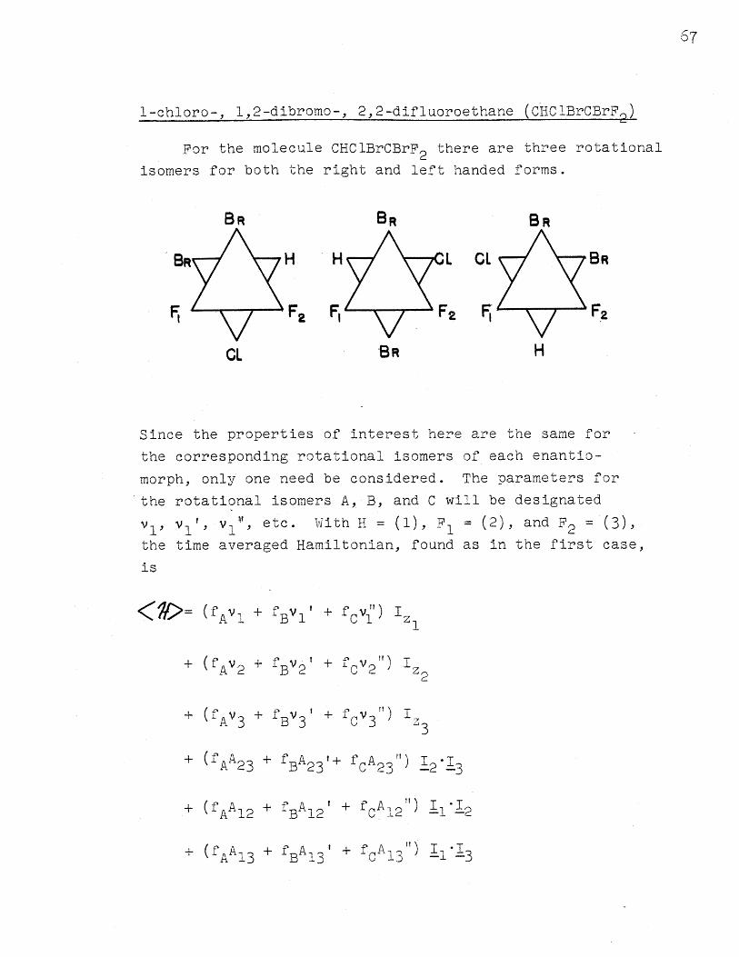
67
1-chloro-, 1,2-dibromo-, 2,2-difluoroethane (CHC1BrCBrF2)
For the molecule CHCIBrCBrP2 there are three rotational
isomers for both the right and left handed forms.
BR
BR H
F,CL
BR
H L
F, F2
BR
BR
CL BR
Fv Fz
H
Since the properties of interest here are the same for
the corresponding rotational isomers of each enantio-
morph, only one need be considered. The parameters for
the rotational isomers A, B, and C will be designated
v1 1 1 , etc. With H = (1), F= (2), and F2 (3),
the time averaged Hamiltonian, found as in the first case,
is
<~ (fAVl + fBVl' + fc') I
+ (fA 2 + fBv 22 + fc 2 ') 2 z 2
+ (fAv3 + fV3v + fcv3 ) ),(fA 3 B 3 c3 3
43
+ (fA'23 + fBA23,+ fCA 231 1) I2 3
+ (fAAl2 BAl2 2 CA 2 ) .12
+ (fAA + fBA 3 ' + fcAl 31 ) 1113A '13 B13 -3L
68
In this case the averaged Hamiltonian has the same form
as that for any single rotational isomer. There is no
reason to expect 2 and 3 to have the same chemical shift
or the same spin-spin coupling to 1. Here there is a
large number of parameters involved in describing the
average spin system and there are three different energies
involved, rather than two. There are enough unknowns
so that little can be done except to show that the
values (Al2 )obs, (A13 )obs, and (v3-v2)obs change with
temperature.
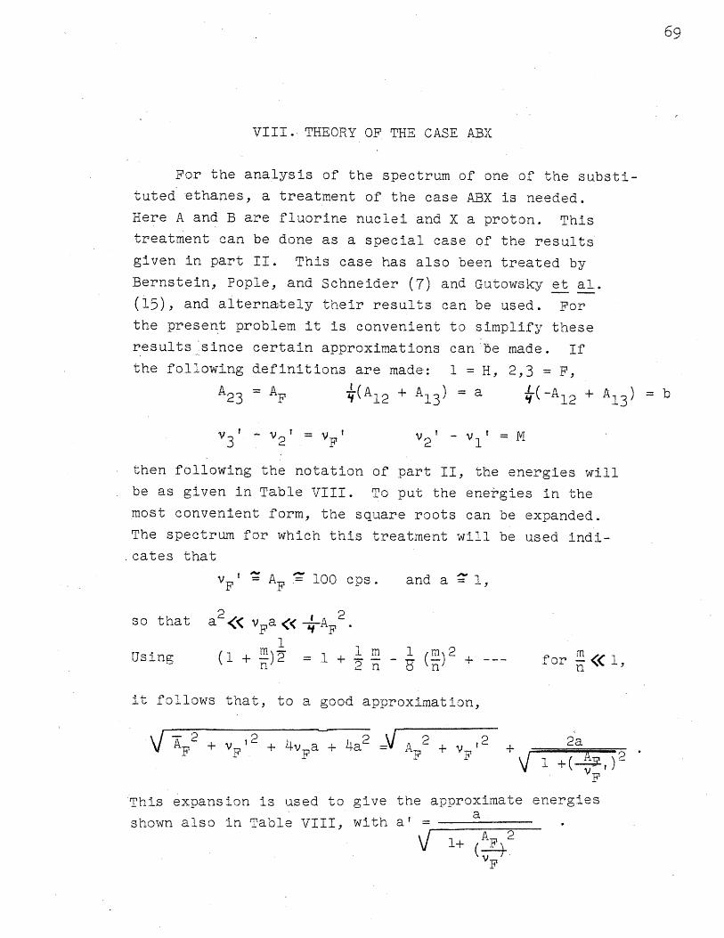
69
VIII. THEORY OF THE CASE ABX
For the analysis of the spectrum of one of the substi-
tuted ethanes, a treatment of the case ABX is needed.
Here A and B are fluorine nuclei and X a proton. Thistreatment can be done as a special case of the results
given in part II. This case has also been treated by
Bernstein, Pople, and Schneider (7) and Gutowsky et al.
(15), and alternately their results can be used. For
the present problem it is convenient to simplify these
results since certain approximations can be made. If
the following definitions are made: 1 = H, 2,3 = F,A2 3 = AF (AI 2 + AI 3 ) = a (-A12 + A13 ) = b
V3 ' - '=MS- v 2 F 2 1 = M
then following the notation of part II, the energies will
be as given in Table VIII. To put the energies in themost convenient form, the square roots can be expanded.
The spectrum for which this treatment will be used indi-.cates that
VF ' A, 100 cps. and a 1',
2 2so that a 2 <( v Fa (< -AF
1 1m 1 m2 rnUsing (1 + ) 2 n ~) + --- for ( I 1
it follows that, to a good approximation,
V /2 ,2 Fa + 2 A 2 2 2aV? + 4 aF F +( )2
VF
This expansion is used to give the approximate energiesa
shown also in Table VIII, with a' =
1+ F 2vr3
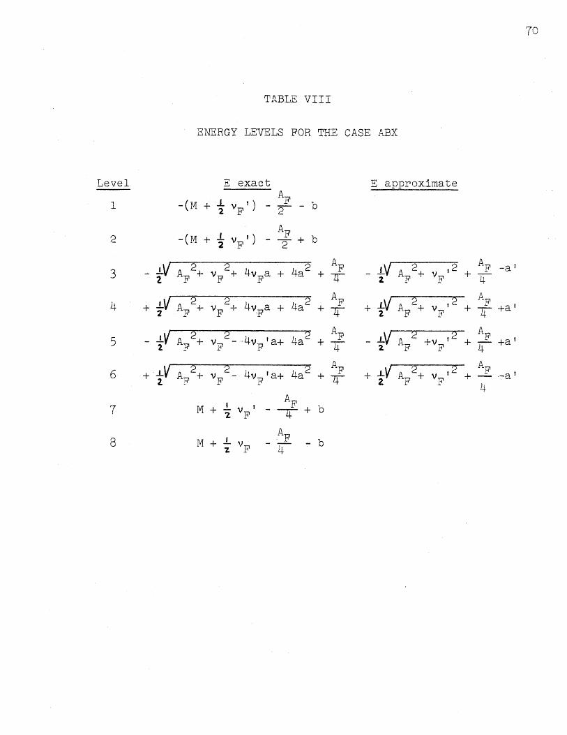
70
TABLE VIII
ENERGY LEVELS FOR THE CASE ABX
E exactA,
-(M + vF') - --(M + 1 ~ ') 2 b
2 F 2
3 - A 2 + v 2+ 4 v a + 4a2 F F F
4 + I A 2 2+ 4v a + 2a422 F F F
5 - A 2+ v 2-- 4 v 'a+ 4a 26 + F F
6 + IV A" 2 + V 2 _ 4 v 'a+ 4a 2
E approximate
A AAF A 2 ± ,2 AF2 F 4
+ L A 2 ,2Z F F
-a'
pT
F - A ' ,2 F
+ Af- + V F ,7 +A
M + v F T +
S AFM+z
z F Lt
A?I-a'
Level
1
8
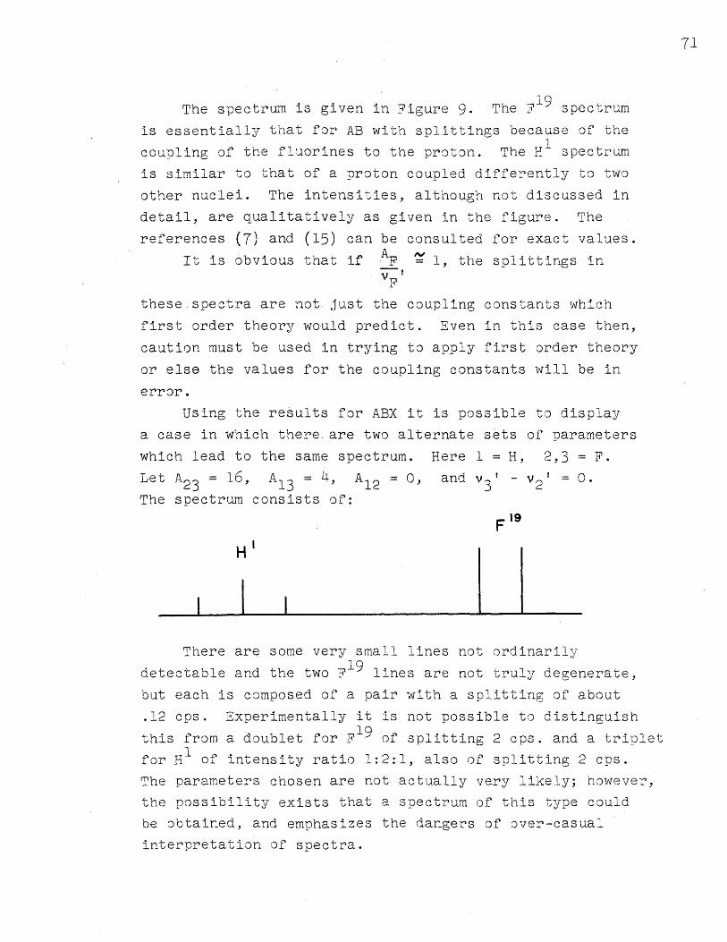
19The spectrum is given in Figure 9. The F spectrum
is essentially that for AB with splittings because of the
coupling of the fluorines to the proton. The Hý spectrum
is similar to that of a oroton coupled differently to two
other nuclei. The intensities, although not discussed in
detail, are qualitatively as given in the figure. The
references (7) and (15) can be consulted for exact values.
It is obvious that if F 1i, the splittings in
F
these spectra are not just the coupling constants which
first order theory would predict. Even in this case then,
caution must be used in trying to apply first order theory
or else the values for the coupling constants will be in
error.
Using the results for ABX it is possible to display
a case in which there are two alternate sets of oarameters
which lead to the same spectrum. Here 1 = H, 2,3 = F.
Let A2 3 = 16, A13 = 4, A1 2 = 0, and 3 - 2 = 0.
The spectrum consists of:
F 9
H
There are some very small lines not ordinarily
detectable and the two F19 lines are not truly degenerate,
but each is composed of a pair with a splitting of about
.12 cps. Experimentally it is not possible to distinguish10
this from a doublet for F9 of splitting 2 cps. and a triplet
for H of intensity ratio 1:2:1, also of splitting 2 cps.The parameters chosen are not actually very likely; however,
the possibility exists that a spectrum of this type could
be obtained, and emphasizes the dangers of over-casual
interpretation of spectra.
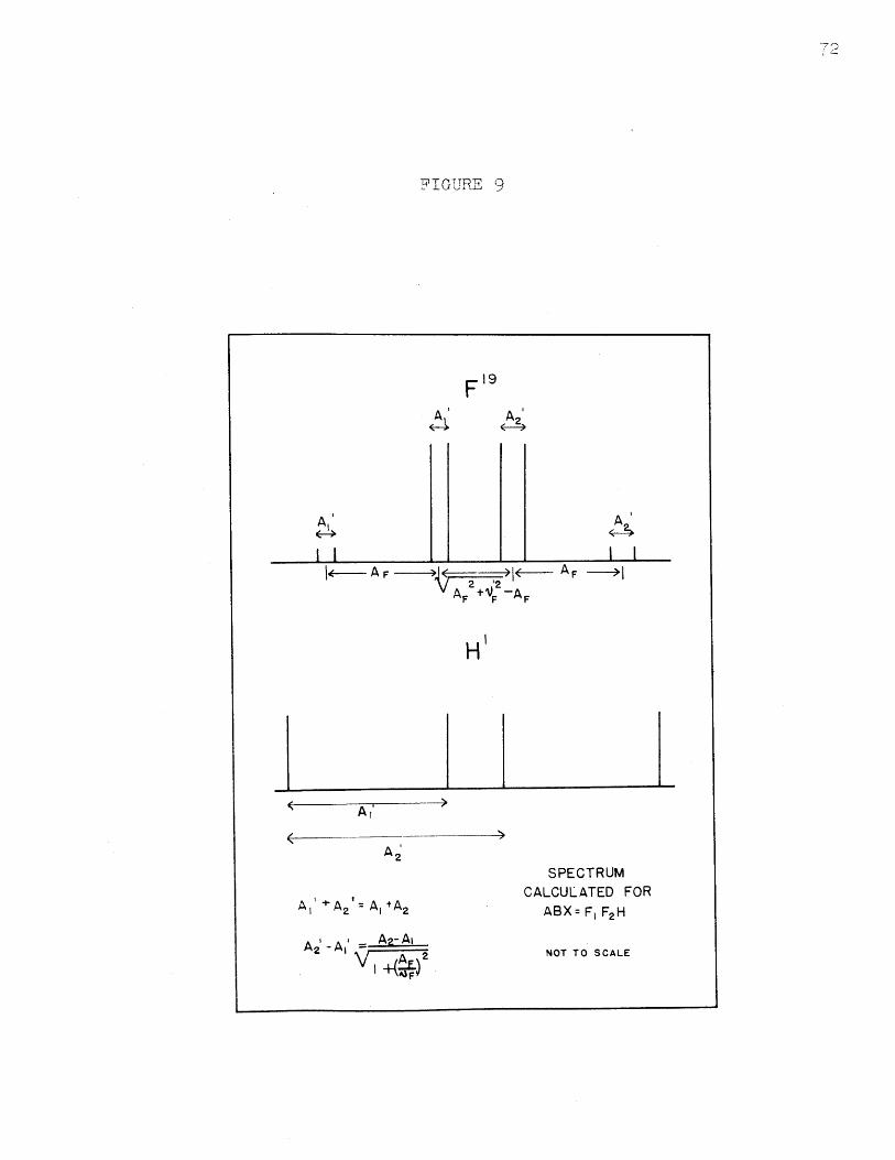
FIGURE 9
IX EXPERIMENTAL
The 1,1,2-trichloro-, 2,2-difluoroethane was prepared
by adding chlorine to 1-chloro-, 2,2-difluoroethylene
(procured from General Chemicals Division, Allied Chemical
and Dye Corporation) in the gas phase. To increase the
speed of the reaction an ordinary 150 watt light bulb was
placed near the reaction vessel. The light bulb was oper-
ated from a Variac to control its actinic output, and
therefore the rate of the reaction. The progress of the
reaction was observed by means of the pressure in the
reaction vessel (1/2 atmosphere) as indicated by a manom-
eter. The chlorine was added as the reaction progressed
so that the CF2=CHC1 was always in excess, in order to
reduce the amount of substitution and to prevent the reac-
tion from proceeding too rapidly. The nuclear resonance19 1
spectrum, just a doublet for F and a triplet for HI
gave no indication of more than one product, assuring that
no substitution had occurred. A distillation in vacuo
easily isolated the product because it boils (at one atmos-
phere) at about 700 C., whereas the reactants boil consid-
erably below 0O C. The sample was sealed into a 5 mm.
O. D. Pyrex tube while under vacuum.
The l-chloro-, 1,2-dibromo-, 2,2-difluoroethane was
prepared by adding bromine to l-chloro-, 2,2-difluoro-
ethylene (same source as above). In this case, the 150
watt light bulb was operated at about 1l40 volts. The
whole amount of bromine was added initially and allowed to
react. The amount was adjusted so that it reacted com-
pletely, allowing easy separation of the product. Again
the spectrum indicated that essentially one compound was
present. The sample was sealed into a 5 mm. O. D. tube.
Both samples exhibited boiling points near those
reported in the literature. 1,1,2-trichloro-, 2,2-difluoro-
ethane boiled near 700 C. (literature value 720 (18) ).
The freezing point for this compound, observed by the
disappearance of all narrow lines in the nuclear resonance
spectrum, was -60° C. - 100. The other compound was
found to boil near 1200 C. (literature, 1180 (18) ), and
the freezing point was observed to be -700 C. i 100.
All the spectra were taken at 40 Mc. with conven-
tional Varian equipment. The slow passage measurements
were all done by the side band technique mentioned earlier
(Section III). Here two audio frequencies were mixed
and used to produce side bands. In this way it is
possible to record only a portion of the spectrum con-
taining two side bands bracketing the other lines of
interest. The known frequency difference between the
two side bands serves as an accurate calibration of
sweep rate. In this way it is possible to scan only
a small portion of the spectrum and to reduce considerably
errors due to changes in the sweep rate. Some care must
be exercised to identify correctly all the lines recorded.
For the measurements of line seoarations of the order
of 5 cycles per second, Reilly's "wiggle beat" method
is ussed (35). (This letter shows some excellent exper-
imental traces.) In this method the pair of lines of
interest is scanned rapidly and the resulting signal
recorded on the Sanborn recorder with a chart speed of 25
or 50 mm./sec. The signal consists of two superimposed
trains of damped oscillations, following the main signal
from the pair of lines. The frequency difference of the
two oscillations will be just the frequency difference
of the two line positions. This frequency difference
appears as the envelope of the resulting train of "wiggles".
The separation between the lines is found thereforeThe , --t nbte elie sfon tee r
75
by comparing the envelope wave length with the distance
between seconds markers on the chart. It is found by
analyzing the errors occurring in a series of measurements
that the probable error in the measurement of a line spacing
can be reduced to .01 cps. or less (in favorable cases) by
averaging 10 or more measurements. The error in the spacing
of the timing markers is about the same, 1 part in 500,
because the markers are derived from the power line frequency.
It is not known whether there are any systematic errors
which increase the absolute error. However, some of the
results presented later indicate that there may be none.
The spectra recorded at other than room temperature
were taken with the sample in the thermostat shown in
Figure 10. To get the resolution desired, the sample
must be rotated about the vertical axis. The rotation
is accomplished by passing the air which maintains the
temperature through a small turbine similar to that used
at.room temperature with the Varian probe.
The temperature range which can be covered is about
-1000 to 2000 C. It is possible to reach lower temperatures
if the sample is not spun.
The operation of the thermostat is as follows. The
air (or tank nitrogen) is passed through either a heater
or cooler, depending upon the temperature desired, into
the thermostat. Because the inlet must be outside the
magnet gap, a rather long dewar tube is provided to carry
the gas to and from the sample. Inside the body of the
thermostat the gas passes through four tangential holes
and onto the surface of the conical turbine, providing
enough torque to spin the sample at 1000 to 2000 r.p.m.d th l th h theThe gas then passes Uownv 11 11. V -1; 1 U L over e samlll 1z; L rougIV L
exit holes, up inside the main dewar, and out through
the dewar tube.
To onerate above room temperature the compressed air
from a laboratory supply line is passed through a heater
before entering the thermostat. The heater consists simply
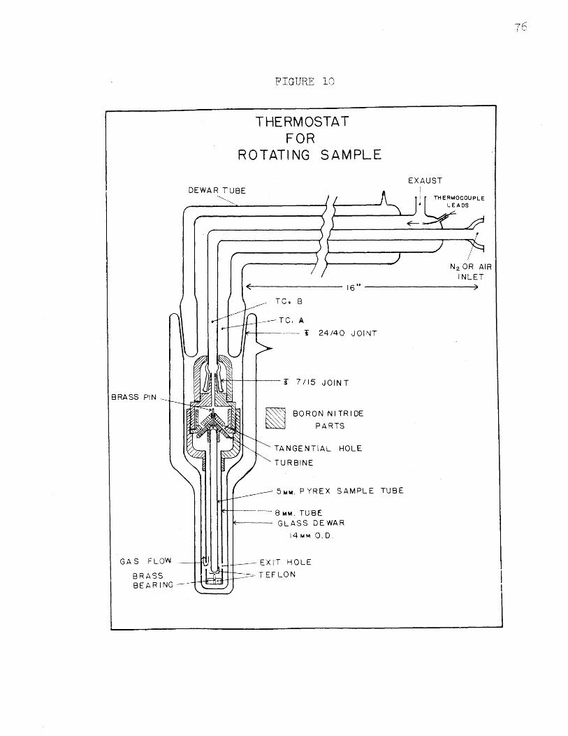
i FIGURE 10
I
i
i
I
I
77
of a coil of nichrome wire inside a glass tube. The wire
is heated by current from a Variac, thereby providing a
means of temperature control. No provision has been made
for automatically regulating the temperature. About 1/2
hour iLs necessary to reach temperature equilibrium.
Below room temperature, tank nitrogen is passed through
a cooler and then through a small heater similar to that
described above. The cooler is a four liter nitrogen
storage dewar equipped with a two-hole cork and containing
liquid nitrogen through which the tank nitrogen is bubbled.
The operation is very similar to that of a bubbler for
washing gases. The only important difference is that
the inlet tube is a dewar tube with a small spiral of
copper tubing on the end. The dewar tube prevents the
incoming gas from warming that leaving at the top of the
flask and the copper tube presumably allows good heat
exchange. The amount of glass wool insulation on the
tubes carrying the cold gas to the thermostat and the
current provided to the small heater are used for providing
temperature control, because the gas flow rate must unfortu-
nately be fixed to obtain proper operation of the turbine
spinning the sample.
The temperature of the sample is measured by copper-
constantan thermocouples at points A and B indicated in
the drawing. The potentials were measured on a recording
potentiometer and are accurate to about the equivalent of
1+ 1 C. At the extremes of temperature there exists a
difference of about 100 between the two points. The
temperature of the sample was assumed to be the average
of the two. The error is estimated to be about /14 of
the temperature difference between points A and B.
The resolution which can be achieved while using the
thermostat is not as good as that possible without it,
probably because there is departure from cylindrical symmetry
in the thermostat which allows the differing diamagnetic
I
susceptibilities of its various parts to produce gradients
in the magnetic field (the most important factor control-
ling the resolution achievable).
X. RESULTS AND DISCUSSION
1,1,2-trichioro-, 2,2-difluoroethane
As was expected, the spectrum for this compound showed19
a simple doublet for the F 1 9 and a triplet of intensity
ratio 1:2:1 for H1. The spacing of the doublet was measured
by the "wiggle beat" method at temperatures between about
-300 C. and 900 C. Below -300 the lines became too wide
for the method to work well. (The wiggle train -became
damped so that only a few cycles of the "beat" were observ-
able.) The widening of the lines can be explained in-part,
at least, by a decreased relaxation time, TI , because of
the lower rate of molecular motions (9);it could also be
caused by the lifetimes of particular rotational isomers
approaching 1 Further work is necessary to decideAH*F
whether the latter is correct. At the highest temperature
the vapor pressure of the sample was about two atmospheres
and it seemed unwise to exceed this.
For each temperature the results of ten or more traces
were averaged; each trace consisted of a train of 8--15
beats. The fairly large number of beats reduced the error
introduced in deciding where the maxima (or minima) of the
beats occurred. The probable error in the average of these
measurements was usually of the order of .01 cps. A proba-
ble error of .005 cps., arising from variations in power
line frequency, should be included in addition to this.
Figure 11 shows the results of the series of measurements.
The heights and widths of the diamonds representing the'
individual points are the probable errors.
The one point taken for H1 (250 c.) agrees very wellwith those for . Because the magnetic field inhomoenwith those for F . Because the magnetic field inhomogen--
ieties controlling the line shape are different for the
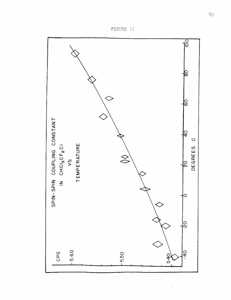
FIGURE ~1
L
two magnetic fields involved, this agreement seems to indi-
cate that the results of this method of measurement do not
depend upon the line shape in any very important way.
Results with the compound discussed later substantiate this.
Unfortunately, the change in (AHF)obs is rather small;
however, it is enough larger than the errors involved to be
meaningful. If the theory of rotational averaging given in
Section VII is accepted, a plot of (AHp)obs against fB'
with the correct value of A E = E - EA used in determining
fB, should be a straight line, within the experimental
error. In the case being discussed here, by choosing differ-
ent values ofAE it is possible to get curves which change
from concave upwards to concave downwards, or vice versa,
depending on the sign of AE. Figures 12 and 13 show plots
of (AHF) obs versus fB (labeled FB in the figures) fordE >0
andAE40; the curves are labeled with 2, 3, or 4, the
value of E for T = 365 ° K. The corresponding values of
AE are 1450, 2200, and 2900 calories/mole. For either sign
of AE the curve labeled 3 is chosen as the best straight
line, for the reason that the proper one seems to lie
between 2 and 4. The absolute value ofAE is then 2200±700
cal./mole. Unfortunately, the energy differences for this
molecule have not been determined by other methods.
IfAE ) the slope is 2g = +5; if E(0 the slope is
2g = -20. To make a comparison with some other results,
the assumption can be made that A' = A, then 2g = A"-A.
Now, in CH2 BrCBrF 2 there are two greatly differing coupling
constants (14, 36). Also the results for substituted
olefins (25) indicate that AHF(trans) _AH(cis) , and it
can be assumed that A"(trans) >A(gauche). If the same wereý
true for CHC12CC1F 2' 2g would be positive, anddE = +2200
would be the proper choice. However, no information exists
which can tell whether A and A" are of the same sign, as
was implicitly assumed above. Because of this fact and
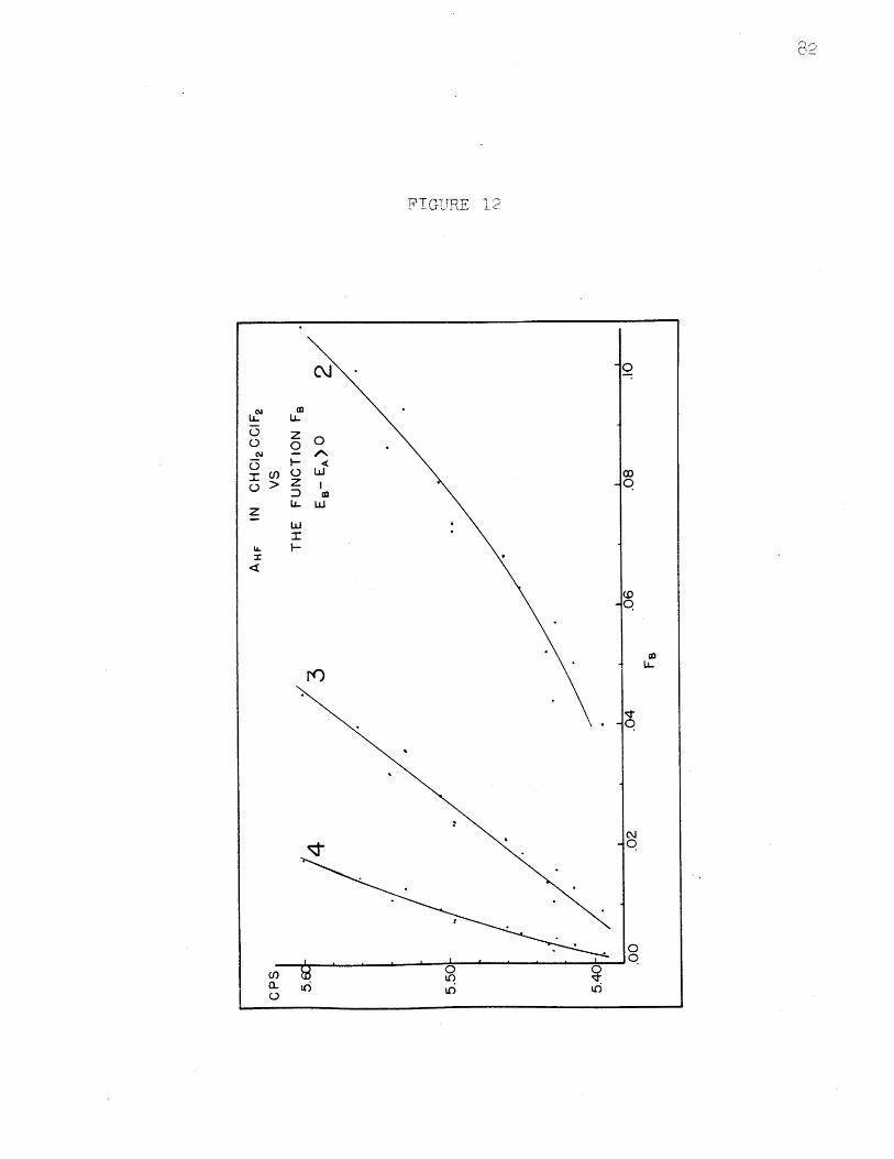
FrGUfrE 12F!iR o
r
ir
ii
1
j
a O 60lj~
rU u"
C) z0ON -
I-I~> Z
LL
<Lz
I
0
0
0
0
oo1
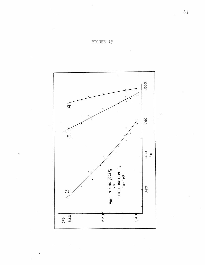
P r!U C3FIGURE 1
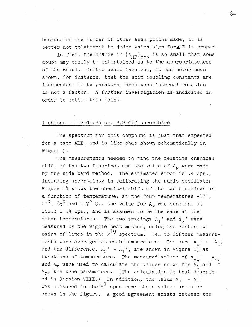
because of the number of other assumptions made, it is
better not to attempt to judge which sign forAE is proper.
In fact, the change in (AHF)obs is so small that some
doubt may easily be entertained as to the appropriateness
of the model. On the scale involved, it has never been
shown, for instance, that the spin coupling constants are
independent of temperature, even when internal rotation
is not a factor. A further investigation is indicated in
order to settle this point.
1-chloro-, 1,2-dibromo-, 2,2-difluoroethane
The spectrum for this compound is just that expected
for a case ABX, and is like that shown schematically in
Figure 9.
The measurements needed to find the relative chemical
shift of the two fluorines and the value of AF were made
by the side band method. The estimated error is .4 cps.,
including uncertainty in calibrating the audio oscillator.
Figure 14 shows the chemical shift of the two fluorines as
a function of temperature; at the four temperatures -17O,
270, 85 and 1170 C., the value for A F was constant at
161.0 _ .4 cps., and is assumed to be the same at the
other temperatures. The two spacings Al' and A2' were
measured by the wiggle beat method, using the center two
pairs of lines in the F1 9 spectrum. Ten to fifteen measure-
ments were averaged at each temperature. The sum, A2 ' + A"and the difference, A2 ' - Afl', are shown in Figure 15 as
functions of temperature. The measured values of v ' - v '2 1and AF were used to calculate the values shown for A and
A2 , the true parameters. (The calculation is that describ-
ed in Section VIII.) In addition, the value A2' - AI
was measured in the H spectrum; these values are also
shown in the figure. A good agreement exists between the
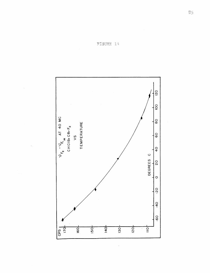
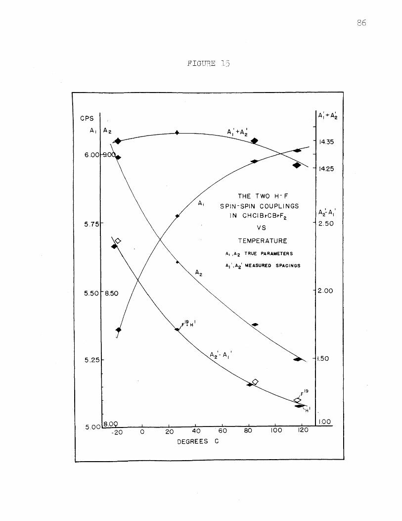
I R86.
.FIGURE 1:-
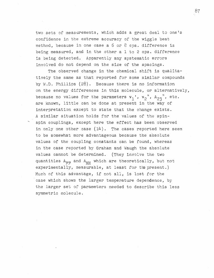
87
two sets of measurements, which adds a great deal to one's
confidence in the extreme accuracy of the wiggle beat
method, because in one case a 6 or 8 cos. difference is
being measured, and in the other a 1 to 2 cps. difference
is being detected. Apparently any systematic errors
involved do not depend on the size of the spacings.
The observed change in the chemical shift is qualita-
tively the same as that reported for some similar compounds
by W.D. Phillips (28). Because there is no information
on the energy differences in this molecule, or alternatively,
because no values for the parameters v1 2 ,' 2 3 etc.
are known, little can be done at present in the way of
interpretation except to state that the change exists.
A similar situation holds for the values of the spin-
spin couplings, except here the effect has been observed
in only one other case (14). The cases reported here seem
to be somewhat more advantageous because the absolute
values of the coupling constants can be found, whereas
in the case reported by Graham and Waugh the absolute
values cannot be determined. (They involve the two
quantities AFF and AHH which are theoretically, but not
experimentally, measurable, at least for the present.)
Much of this advantage, if not all, is lost for the
case which shows the larger temperature dependence, by
the larger set of parameters needed to describe this less
symmetric molecule.
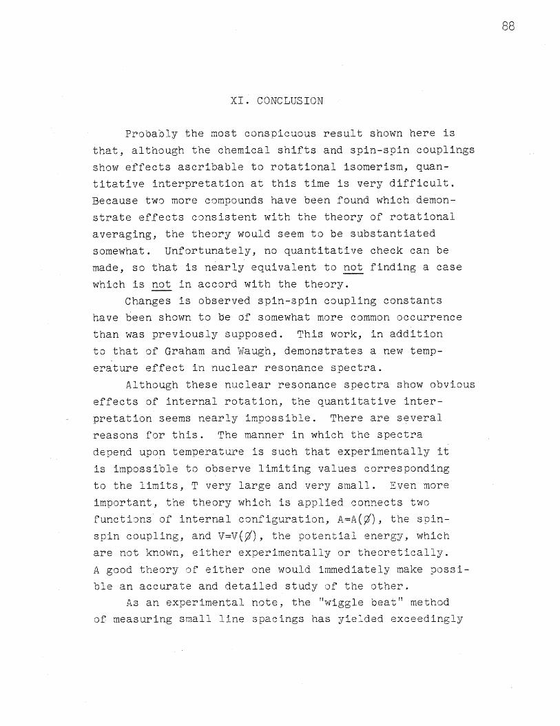
88
XI. CONCLUSION
Probably the most conspicuous result shown here is
that, although the chemical shifts and spin-spin couplings
show effects ascribable to rotational isomerism, quan-
titative interpretation at this time is very difficult.
Because two more compounds have been found which demon-
strate effects consistent with the theory of rotational
averaging, the theory would seem to be substantiated
somewhat. Unfortunately, no quantitative check can be
made, so that is nearly equivalent to not finding a case
which is not in accord with the theory.
Changes is observea spin-spin coupling constants
have been shown to be of somewhat more common occurrence
than was previously supposed. This work, in addition
to that of Graham and Waugh, demonstrates a new temp-
erature effect in nuclear resonance spectra.
Although these nuclear resonance spectra show obvious
effects of internal rotation, the quantitative inter-
pretation seems nearly impossible. There are several
reasons for this. The manner in which the spectra
depend upon temperature is such that experimentally it
is impossible to observe limiting values corresponding
to the limits, T very large and very small. Even more
important, the theory which is applied connects two
functions of internal configuration, A=A('), the spin-
spin coupling, and V=V(/), the potential energy, which
are not known, either experimentally or theoretically.
A good theory of either one would immediately make possi-
ble an accurate and detailed study of the other.
As an experimental note, the "wiggle beat" method
of measuring small line spacings has yielded exceedingly
89
precise results. In particular, the difference between
the measurements of two splittings and the measurement
of that difference itself, as it appeared in another
part of the spectrum, agreed to within the experimental
error. This agreement should help dispel any doubts thatthe accuracy of the method is the same as its precision.
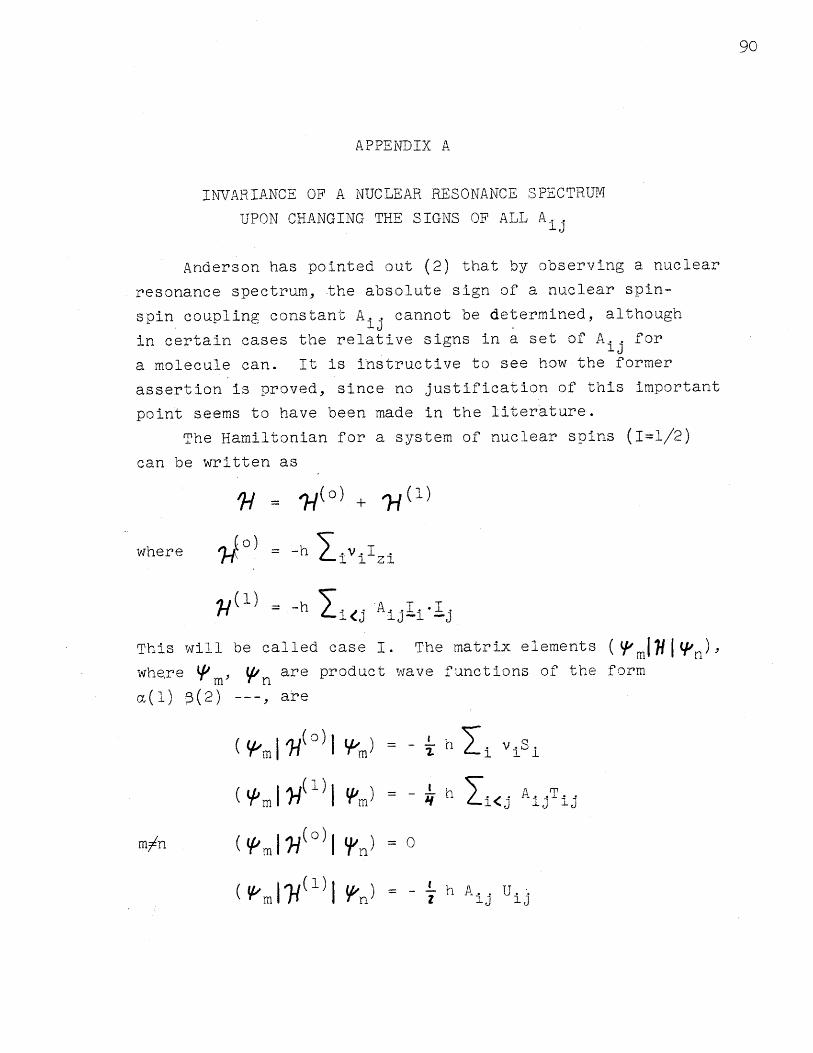
90
APPENDIX A
INVARIANCE OF A NUCLEAR RESONANCE SPECTRUM
UPON CHANGING THE SIGNS OF ALL Aij
Anderson has pointed out (2) that by observing a nuclear
resonance spectrum, t the absolute sign of a nuclear spin-
spin coupling constant A.. cannot be determined, although
in certain cases the relative signs in a set of Aij for
a molecule can. It is instructive to see how the former
assertion is proved, since no justification of this important
point seems to have been made in the literature.h H Ail-t in -M a s stm of niclearsins (T=1 /2)
can be written as
( = o4() + 1-(1)
where (o0) = -h iV iIzi
U(1) = -h ij Aj i'jI
This will be called case I. The matrix elements (fm n) '
where fm, Pn are product wave functions of the form
a(1) ý(2) --- , are
4m() h = - h vSij
m/n ( 7•(o )I 9n) O
( (m 1(1)1 nP) = h -i U jij
i
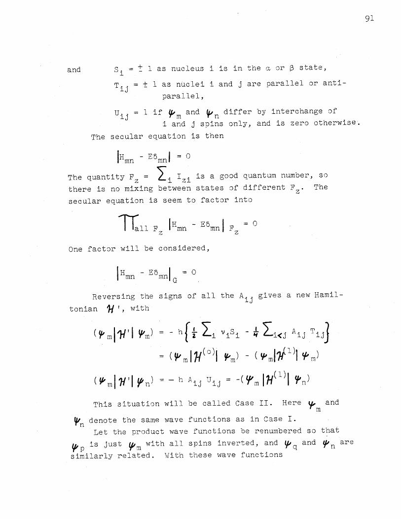
and S. = - 1 as nucleus i is in the a or ý state,
T + 1 as nuclei i and j are parallel or anti-
parallel,
Uij = 1 if m and n differ by interchange of
i and j spins only, and is zero otherwise.
The secular equation is then
SHmn - E5mnI = 0
The quantity F = i i is a good quantum number, so
there is no mixing between states of different Fz . The
secular equation is seem to factor intoi'
TIall F IJmn - E5mn F = 0
One factor will be considered,
I E I OIHmn - UmnlG -
Reversing the signs of all the Aij gives a new Hamil-
tonian 'j ', with
(m m) = - h v Si i<j Ti
3m= (y () m 3m ) m
mn)= -h' • U.. -( (m -l'(.()
This situation will be called Case II. Here Y andm
Wn denote the same wave functions as in Case I.
Let the product wave functions be renumbered so that
is just 'm with all spins inverted, and pq and 'n arep .. . Vo qn
similarly related. With these wave functions
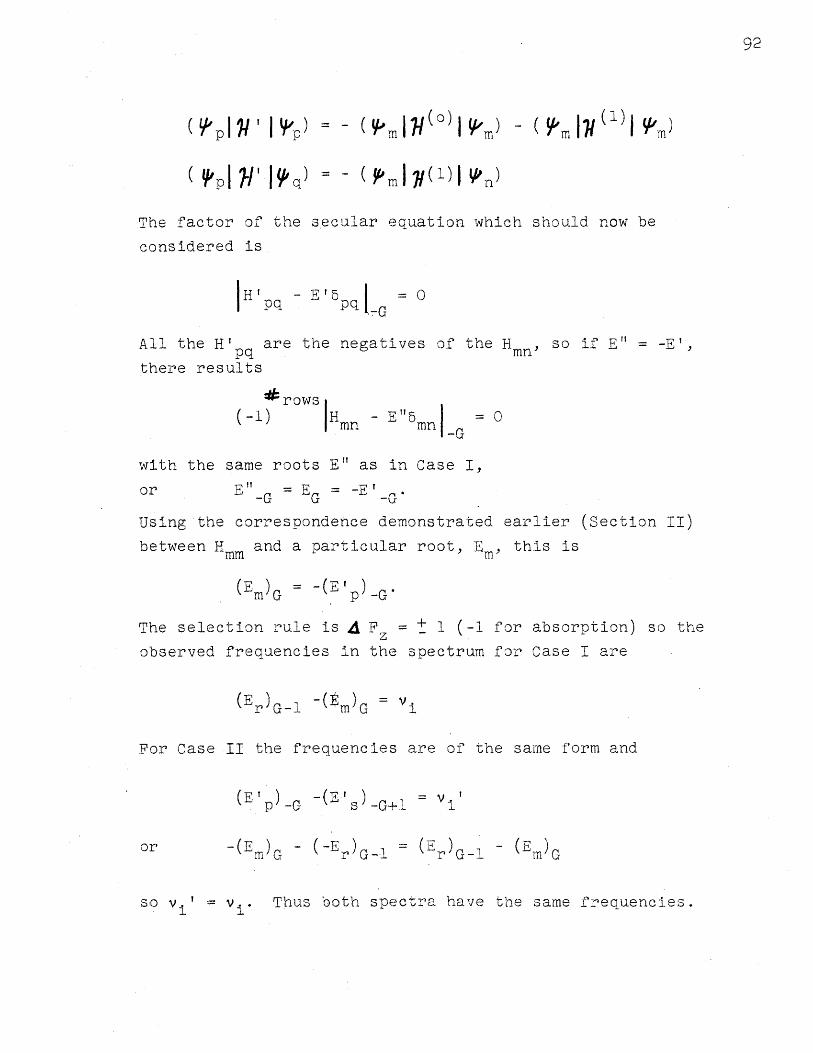
92
-- - -1I'
The factor of the secular equation which should now be
considered is
H' - E' pq Oi Pq -G
All the H'pq are the negatives of the H mn, so if E" = -E',
there results
rows I-k ) mn -E 5mn G
-G
with the same roots E" as in Case I,
or E"G = EG = -E'_G*
Using the correspondence demonstrated earlier (Section I!)
between H and a Darticular root. E . this is.. . .mm
(Em)G = -(E )-G'
The selection rule is 4 Fz = + 1 (-i for absorption) so the
observed frequencies in the spectrum for Case I are
()G-1 -(1m)G = i
For Case II the frequencies are of the same form and
(E' ) -(E' ) = i'
or -(Em) - (-E)l = (EG- - (Em)GmrdG rG-1 r G-1 mG
so vi' v. Thus both spectra have the same frequencies.s is
I

93
To find the intensity of any transition, the stationary
state wave functions for Cases I and II must be found. This
is done as follows for Case I. A proper wave function is
with he amkgiven bk a mkset o homogensous equationsk
with the amk given by a set of homogensous equations
Zk (Hm'k - Emmk ) amk = 0 for each m'
Because of the correspondence between states of Fz
of opposite sign in Cases I and II, there is a proper
wave function for Case II given by
= Zk apk 9W'Th-' r gienb
The a'pk are given by
Zk (H'p'k - E 5p'k) a'ppR = 0
where the /'k are the
Yk with all spins inverted.
for all p'.
But all the elements H'p'k = -Hm'k and E = -Em , as seen in
calculating the Ep. Hence,
(-1) Zk (Hm'k - E mm'k) a pk = 0
or the a'pk are just the amk.The intensity of a transition in Case I is proportional
(r IIx Im) 2 = - k, amkar' x kj
The corresponding transition for Case II is S-- p, and the
intensity is
(w Ix s) 2= [ke akaIOU ska tkx J
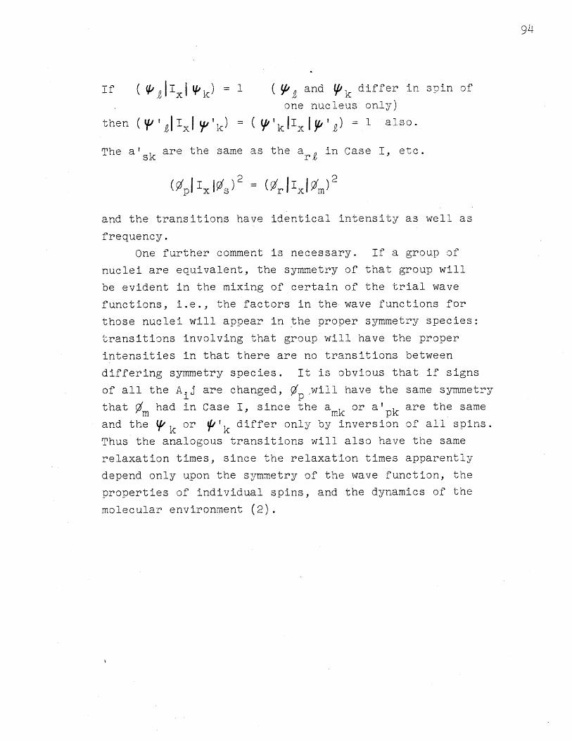
94
If ( Ix k ( and (Pk differ in spin of
one nucleus only)
then (( dlxJ ( lkxI, I ) = 1 also.
The a'sk are the same as the are in Case I, etc.
(/Ixis) 2 :(rIx r m)2
and the transitions have identical intensity as well as
frequency.
One further comment is necessary. If a group of
nuclei are equivalent, the symmetry of that group will
be evident in the mixing of certain of the trial wave
functions, i.e., the factors in the wave functions for
those nuclei will appear in the proper symmetry species:
transitions involving that group will have the proper
intensities in that there are no transitions between
differing symmetry species. It is obvious that if signs
of all the A.j are changed, Jpwill have the same symmetry
that 1( had in Case I, since the amk or a'pk are the same
and the Pk or 'k differ only by inversion of all spins.
Thus the analogous transitions will also have the same
relaxation times, since the relaxation times apparently
depend only upon the symmetry of the wave function, the
properties of individual spins, and the dynamics of the
molecular environment (2).
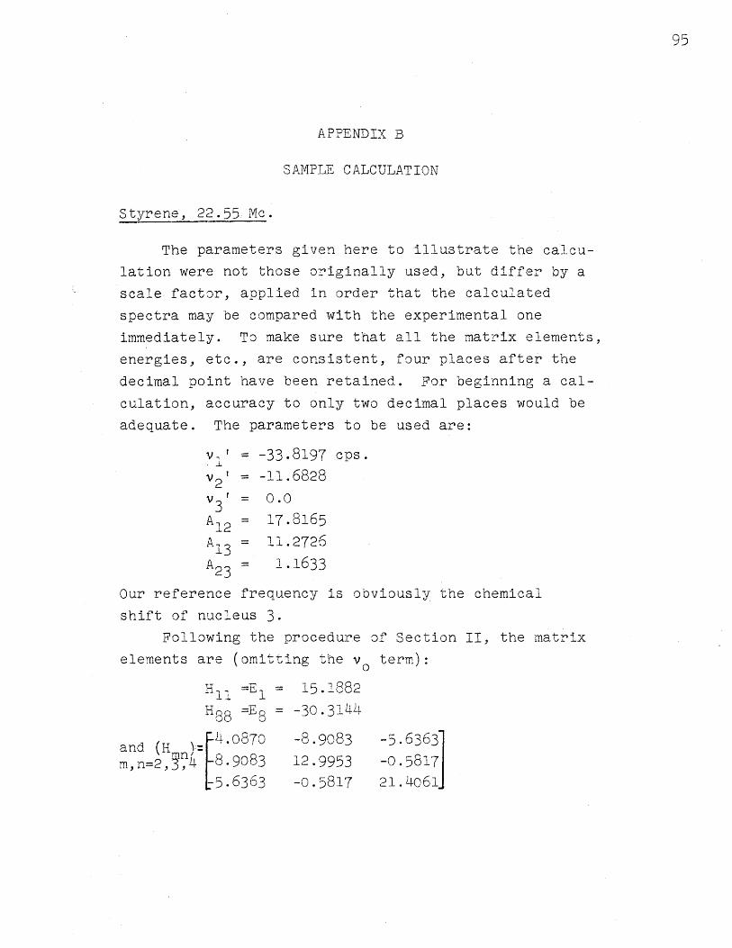
APPENDIX B
SAMPLE CALCULATION
Styrene, 22.55 Mc.
The parameters given here to illustrate the calcu-
lation were not those originally used, but differ by a
scale factor, applied in order that the calculated
spectra may be compared with the experimental one
immediately. To make sure that all the matrix elements,
energies, etc., are consistent, four places after the
decimal point have been retained. For beginning a cal-
culation, accuracy to only two decimal places would be
adequate. The parameters to be used are:
1 ' -33.8197 cps.
' = -11.68282
v ' 0.03A2 = 17.8165
A = 11.272613
A = 1.163323
Our reference frequency is obviously the chemical
shift of nucleus 3.
Following the procedure of Section II, the matrix
elements are (omitting the v0 term):
H 1 =E = 15.1882
H8 8 =E8 -30.3144
-40and ( 870 -8.9083 -5.6363mn=2,.n4 8.9083 12.9953 -0.5817
5.6363 -0.5817 21.4061o
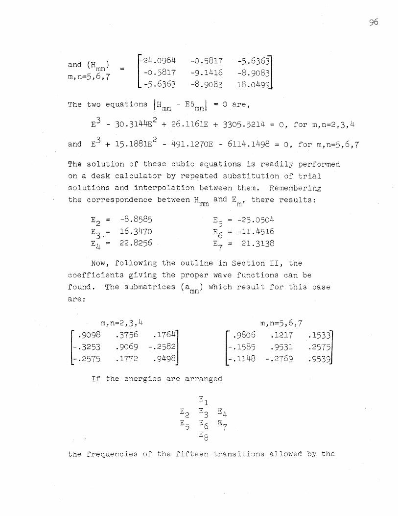
and (H mn)
m,n=5,6,7
-24.0964-0.5817-5. 6363
-0.5817 -5.63637-9.1416 -8.9o83j
-8.9083 18.0499j
The two equations IHmn - ESmn = 0 are,
E - 30.3144E2 + 26.1161E + 3305.5214 = 0, for m,n=2,3,4
and E 3 + 15.1881E 2 - 491.1270E - 6114.1498 = 0, for m,n=5,6,7
The solution of these cubic equations is readily performed
on a desk calculator by repeated substitution of trial
solutions and interpolation between them. Remembering
the correspondence between H1 mm and E , there results:mm m
E2 = -8.8585
E = 16.3470
4 = 22.8256
E5 = -25.0504
E6 = -1.4516
E7 = 21.3138
Now, following the outline in Section II, the
coefficients giving the proper wave functions can be
found. The submatrices (amn) which result for this case
are:
m,n=2,3,4
.3756 .1764
.9069 -.25821
.1772 .9498J
m,n=5,6,7
S.9806 .1217 .1533.1585 .9531 .2575i
-.1148 -.2769 .9539J
If the energies are arranged
E1E2 E3 E4E E 7
the frequencies of the fifteen transitions allowed by the
96
.9098
-. 3253
-. 2575
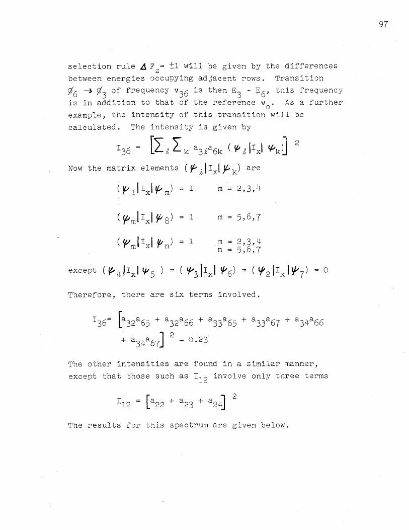
97
selection rule 4 F = +1 will be given by the differences
between energies occupying adjacent rows. Transition
6 -, 63 of frequency v3 6 is then E3 - E6, this frequency
is in addition to that of the reference vo. As a further
example, the intensity of this transition will be
calculated. The intensity is given by
136= a3 6k (, 2fkk a361 (2
Now the matrix elements (~- IxlIk) are
!(flIxIm) = 1 m = 2,3,4
( mllxl 8") 1= m = 5,6,7
(mlixi n ) = 1 m = 2,3,4
n = 5,6,7
except (iJ-41xl ) = ( '3IxI V'6) = ( 2 x VIL ' 7 ) = 0
Therefore, there are six terms involved.
136= [a 3 2 a 6 5 + a 3 2 a 6 6 + a 3 3 a 6 5 + a33a67 + a 3 4 a 6 6
+ a34 a67 = 0.23
The other intensities are found in a similar manner,
except that those such as 112 involve only three terms
112 = a 2 2 + a 2 3 + a 2 2
The results for this spectrum are given below.
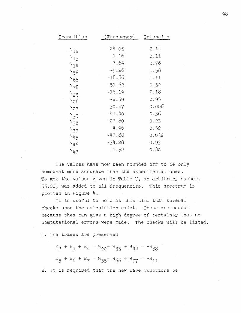
Transition
v 1 2
V13v 1 4
v 5 8V6 8v 7 8V2 5v 2 6
v 2 7v 3 5
v360V3 7
v 4 5
v 4 6
v 4 7
-(Frequency) Intensity
-24.05
1.167.64
-5.26-18.86
-51.62
-16.19
-2.59
30.17-41.40o
-27.804.96
-47.88
-34.28-1.52
2.14
0.11
0.761.58
0.322.18
0.95o.oo60.36
0.230.52
0.0320.93
0.80
The values have now been rounded off to be only
somewhat more accurate than the experimental ones.
To get the values given in Table V, an arbitrary number,
55.00, was added to all frequencies. This spectrum is
plotted in Figure 4.
It is useful to note at this time that several
checks upon the calculation exist. These are useful
because they can give a high degree of certainty that no
computational errors were made. The checks will be listed.
1. The traces are preserved
E2 + E 3 + E = H2 2 + H3 3 + H 4 4 = -H 88
5 + E6 + E H + H + H 7 7 = -H 1l
2. It is required that the new wave functions be
98
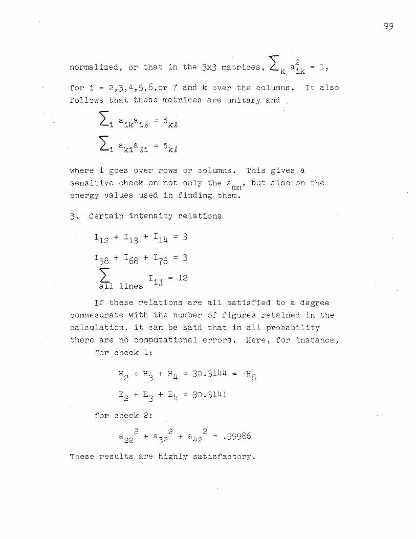
99
2
normalized, or that in the 3x3 matrices, k k = 1,
for i = 2,3,4,5,6,or 7 and k over the columns. It also
follows that these matrices are unitary and
ai aia = 5i ik i' ki
i akiai = 6k£
where i goes over rows or columns. This gives a
sensitive check on not only the amn, but also on the
energy values used in finding them.
3. Certain intensity relations
112 113 + 114 = 3
158 + I68 +78 = 3
i =12all lines
If these relations are all satisfied to a degree
commesurate with the number of figures retained in the
calculation, it can be said that in all probability
there are no comoutational errors. Here, for instance,
for check 1:
H2 + H3 + H4 = 30.3144 -H8
E 2 + E + E = 30.3141
for check 2:
2 2 2a2 2 + a32 + a 2 = .9986
These results are highly satisfactory.
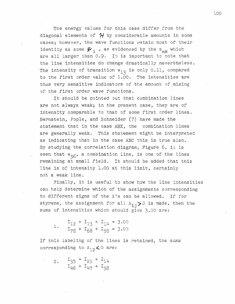
100
The energy values for this case differ from the
diagonal elements of 14 by considerable amounts in some
cases; however, the wave functions retain most of their
identity as some Pi , as evidenced by the amm which
are all larger than 0.9. It is important to note that
the line intensities do change drastically nevertheless.
The intensity of transition v13 is only 0.11, compared
to the first order value of 1.00. The intensities are
thus very sensitive indicators of the amount of mixing
of the first order wave functions.
It should be pointed out that combination lines
are not always weak; in the present case, they are of
intensity comparable to that of some first order lines.
Bernstein, Pople, and Schneider (7) have made the
statement that in the case ABX, the combination lines
are generally weak. This statement might be interpreted
as indicating that in the case ABC this is true also.
By studying the correlation diagram, Figure 6, it is
seen that v36 , a combination line, is one of the lines
remaining at small field. It should be added that this
line is of intensity 1.00 at this limit, certainly
not a weak line.
Finally, it is useful to show how the line intensities
can help determine which of the assignments corresponding
to different signs of the A's can be allowed. If for
styrene, the assignment for all Aij20 is made, then the
sums of intensities which should give 3.00 are:
T12 +13 + I = 3.00
. 78 + I68 + I58 = 3.00
If this labeling of the lines is retained, the sums
corresponding to A12 <O are:
2. 35 + 125 + 14146 + 47 + I58
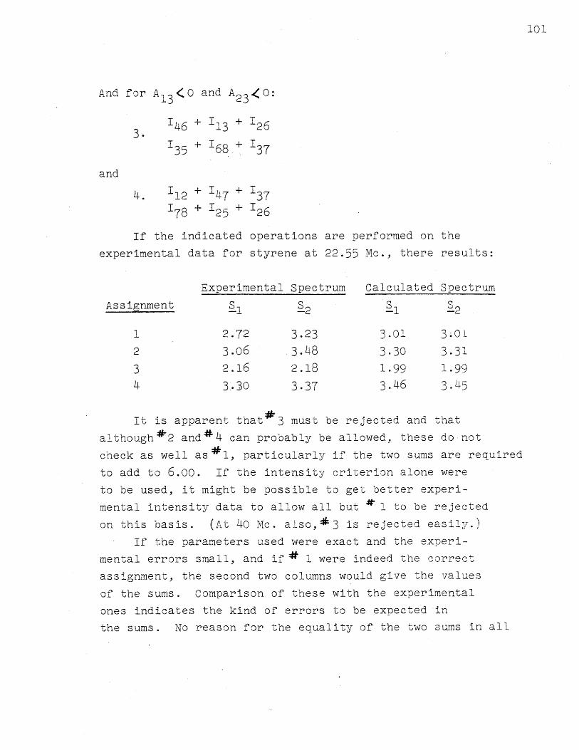
101
And for A13 <O and A23 0:
146 + 113 + 126
135 + 168.+ 137
and
4. 112 + 147 + 137
178 + 125 + 126
If the indicated operations are performed on the
experimental data for styrene at 22.55 Mc., there results:
Experimental Spectrum Calculated Spectrum
Assignment S S2 S S
1 2.72 3.23 3.01 3.01
2 3.06 3.48 3.30 3.31
3 2.16 2.18 1.99 1.99
4 3.30 3.37 3.46 3.45
It is apparent that*3 must be rejected and that
although*2 and *4 can probably be allowed, these do not
check as well as 1, particularly if the two sums are required
to add to 6.00. If the intensity criterion alone were
to be used, it might be possible to get better experi-
mental intensity data to allow all but 1~ to be rejected
on this basis. (At 40 Mc. also,*3 is rejected easily.)
If the parameters used were exact and the experi-
mental errors small, and if * 1 were indeed the correct
assignment, the second two columns would give the values
of the sums. Comparison of these with the experimental
ones indicates the kind of errors to be expected in
the sums. No reason for the equality of the two sums in all
102
cases (although they do not now equal 3.00) has been
found, but this fact and the deviations between ideal
and observed sums would strongly suggest that 1
is the only assignment which can be accepted.
103
LITERATURE CITED
1. Alexander, S. J. Chem. Phys. 28, 358 (1958).
2. Anderson, W.A. Phys. Rev. 102, 151 (1956).
3. Anderson, W.A., and J.T. Arnold. Phys. Rev. 94,497 (1954).
4. Arnold, J.T. Phys. Rev. 102, 136 (1956).
5. Baker, E.B. J. Chem. Phys. 26, 960 (1957).
6. Banerjee, M.K., T.P. Das, and A.K. Saha. Proc. Roy.Soc. A 226, 490 (1954).
7. Bernstein, H.J., J.A. Pople, and W.G. Schneider.Can. J. Chem. 35, 65 (1957).
8. Bloch, F. Phys. Rev. 94, 496 (1954).
9. Bloembergen, N., E.M. Purcell, and R.V. Pound.Phys. Rev. 73, 679 (1948).
10. Bohm, D. Quantum Theory. (Prentice-Hall Inc., NewYork, 1951.) Chapter 16.
11. Corio, P;a, and B.P. Dailey. J. Am. Chem. Soc. 78,3043 (1956).
12. Drysdale, J.J., and W.D. Phillips. J. Am. Chem. Soc.79, 319 (1957).
13. Edmonds, A.R. Angular Momentum in Quantum Mechanics.(Princeton Univ. Press, 1957). Chapter 2.
14. Graham, D.M., and J.S. Waugh. J. Chem. Phys. 27,468 (1957).
15. Gutowsky, H.S., C.H. Holm, A. Saika, and G.A. Williams.J. Am. Chem. Soc. 79, 4596 (1957).
16. Gutowsky, H.S., D.W. McCall, and C.P. Slichter.J. Chem. Phys. 21, 279 (1953).
17. Hahn, E.L., and D.E. Maxwell. Phys. Rev. 88, 1070 (1952).
18. Henne, A.L., and E.C. Ladd. J. Am. Chem. Soc. 58 ,402 (1936).
19. Karplus, M., D.H. Anderson, T.C. Farrar, and H.S.Gutowsky. J. Chem. Phys. 27, 597 (1957).
20. Lee, J., and L.H. Sutcliffe. Trans. Far. Soc. 54,308 (1958).
21. McConnell, H.M. J. Chem. Phys. 24, 460 (1956).

o104
22. McConnell, H.M. J. Mol. Spec. 1, 11 (1957).
23. McConnell, H.M., and W.A. Anderson. J. Chem. Phys. 26,496 (1957).
24. McConnell, H.M., A.D. McLean, and C.A. Reilly.J. Chem. Phys. .23, 1152 (1955).
25. McConnell, H.M., C.A. Reilly, and A.D. McLean.J. Chem. Phys. 24, 479 (1956).
26. Mizushima, S. Structure of Molecules and InternalRotation. (Acad. Press, Inc., N.Y. 1954).
27. Nair, P.M., and J.D. Roberts. J. Am. Chem. Soc. 79,4564 (1957).
28. Phillips, W. D. Reported at the Nov. 22, 1957 meetingof the New York Academy of Sciences. To be published.
29. Pople, J.A. Molec. Physics, 1, 1 (1958).
30. Pople, J.A., W.G. Schneider, and H.J. Bernstein.Can. J. Chem. 35, 1060 (1957).
31. Quinn, W.E., and R.M. Brown. J. Chem. Phys. 21,1605 (1953).
32. Ramsey, N. Phys. Rev. 78, 699 (1950).
83, 540 (1951).86, 242 (1952).
33. Ramsey, N. Ibid. 91, 303 (1953).
34. Ramsey, N., and E.M. Purcell. Phys. Rev. 85, 143 (1952).
35. Reilly, C.A. J. Chem. Phys. 25, 604 (1956).
36. Shoolery, J.N., and B. Crawford, Jr. J. Mol. Spec.
1, 270 (1957).37. Waugh, J.S., and R.W. Fessenden. J. Am. Chem. Soc.
79, 846 (1957).
38. Williams, G.A., and H.S. Gutowsky. Phys. Rev.104, 278 (1956).
105
BIOGRAPHY OF THE AUTHOR
Richard Warren Fessenden, son of Mr. and Mrs.
Richard William Fessenden, was born on January 22, 1934,
in Northampton, Massachusetts. He attended the public
schools of Amherst, Massachusetts, graduating from high
school in June, 1951.
He attended the University of Massachusetts from
June, 1951, to February, 1955, during which time he was
selected as Phi Kappa Phi Class Scholar in three
sucessive years and as Phi Beta Kappa Class Scholar,
and was elected a member of Phi Kappa Phi and Sigma
Xi. He graduated Summa cum laude with a B. S. Degree
in June, 1955.
In February, 1955, he enrolled as a candidate
for the degree of Doctor of Philosophy in Physical
Chemistry at the Massachusetts Institute of Technology.
He held a National Science Foundation Fellowship in
the academic years 1956-1957 and 1957-1958. While
at M. I. T. he was elected a full member of Sigma Xi.
He accepted a National Science Foundation Postdoctoral
Fellowship for study at the California Institute of
Technology for a year, starting in September, 1958.


![Sarah Fessenden to Sally [Fessenden - Bowdoin LibraryWm. Fessenden to Sarah Fessenden Boston, June 10, 1801 S[amuel] Fessenden to Mary [P. Fessenden] Hanover, November 17, 1803 Samuel](https://img.pdfslide.us/doc/110x75/608819cd6150d8086253735f/sarah-fessenden-to-sally-fessenden-bowdoin-library-wm-fessenden-to-sarah-fessenden.jpg)