Note: Within nine months of the publication of the mention of the grant of the European patent in the European PatentBulletin, any person may give notice to the European Patent Office of opposition to that patent, in accordance with theImplementing Regulations. Notice of opposition shall not be deemed to have been filed until the opposition fee has beenpaid. (Art. 99(1) European Patent Convention).

Printed by Jouve, 75001 PARIS (FR)

(19)E

P2

466

568

B1

TEPZZ 466568B_T(11) EP 2 466 568 B1

(12) EUROPEAN PATENT SPECIFICATION

(45) Date of publication and mention of the grant of the patent: 26.06.2013 Bulletin 2013/26

(21) Application number: 11425301.6

(22) Date of filing: 19.12.2011

(51) Int Cl.:G08G 5/00 (2006.01) G05D 1/06 (2006.01)

(54) A fast vertical trajectory prediction method for air traffic management, and relevant ATM system

Schnelles Vorhersageverfahren für eine vertikale Flugbahn für Luftverkehrsmanagement, und relevantes ATM-System

Procédé de prédiction de trajectoire verticale rapide pour la gestion du trafic aérien et système ATM correspondant

(84) Designated Contracting States: AL AT BE BG CH CY CZ DE DK EE ES FI FR GB GR HR HU IE IS IT LI LT LU LV MC MK MT NL NO PL PT RO RS SE SI SK SM TR

(30) Priority: 20.12.2010 IT RM20100672

(43) Date of publication of application: 20.06.2012 Bulletin 2012/25

(73) Proprietor: SELEX ES S.P.A00187 Roma (RM) (IT)

(72) Inventors: • Accardo, Domenico

80125 Napoli (IT)• Moccia, Antonio

80125 Napoli (IT)• Grassi, Michele

80125 Napoli (IT)• Tancredi, Urbano

80143 Napoli (IT)• Caminiti, Lucio

00131 Roma (IT)

• Fiorillo, Luigi80070 Bacoli (NA) (IT)

• Leardi, Alberto00131 Roma (IT)

• Maresca, Giuseppe80014 Giugliano (NA) (IT)

(74) Representative: Perronace, Andrea et alBarzano & Zanardo Roma S.p.A. Via Piemonte 2600187 Roma (IT)

(56) References cited: WO-A2-2007/072028

• MANOLAKIS D E: "Aircraft vertical profile prediction based on surveillance data only", IEE PROCEEDINGS: RADAR, SONAR & NAVIGATION, INSTITUTION OF ELECTRICAL ENGINEERS, GB, vol. 144, no. 5, 1 October 1997 (1997-10-01), pages 301-307, XP006008926, ISSN: 1350-2395, DOI: DOI:10.1049/IP-RSN:19971210

EP 2 466 568 B1

2

5

10

15

20

25

30

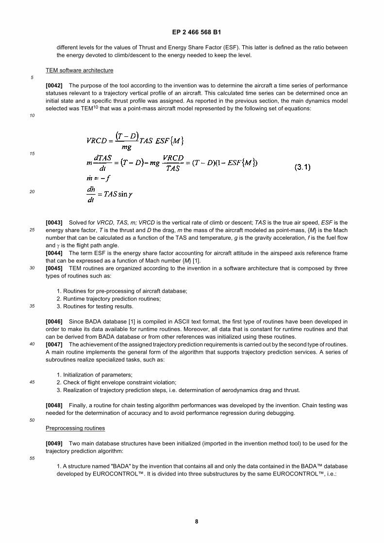
35

40

45

50

55

Description

[0001] The present invention concerns a fast vertical trajectory prediction method for air traffic management (ATM),and relevant ATM system.[0002] More in detail, the present invention concerns a method which is able to calculate the vertical trajectory of anaircraft, by integrating in a suitable way numerical solutions and analytical solutions for some flight phases, in a fast andcomputationally effective way. The present invention further concerns an ATM system implementing the method of theinvention.[0003] ATM systems are currently supporting flights. However, the relevant international traffic is increasing rapidly[4,5] and the need is felt for an ATM systems that support a number of flights that is much larger than the one of currentoperative systems.[0004] Therefore, the automation level in ATM processes must be increased to fulfill this requirement. The number ofaircrafts that are planned to fly in the next generation airspace would require a non realistic number of human controllers[6]. As a consequence, software controllers would replace human ones in the main function such as conflict resolution.[0005] Several tools are under development to support the implementation of safe software controllers. Indeed, somefunctions require running complex algorithms with a heavy computational load. Moreover, since a real time solution isneeded, these algorithms should be adequate to ensure the output of a solution in a short time. In particular, uncontrolledloops must be avoided, since they prevent the system to fulfill the requirement for time determinism.[0006] An important class of tools that are needed for future airspace management are conflict resolution systems[4,5]. They need to be supported by accurate trajectory prediction algorithms to generate realistic solutions for detectedin-flight congestions. In the last few years, several tools have been developed to provide effective trajectory prediction[7-11].[0007] The main issues related to the realization of a proper trajectory prediction tool are:

i. The tool must be capable to support real-time conflict resolution, i.e. thousands of runs must be performed in fewseconds;ii. The tool must be based on the knowledge of parameters included in an aircraft database that covers all managedtraffic and that is updated as soon as a non negligible number of new aircraft models is introduced in the market.

[0008] To ensure that condition i) is satisfied, the trajectory prediction computational engine must be reduced so thatit performs the minimum number of needed computations to generate a solution.[0009] Regarding condition ii), the worldwide standard database that was selected as reference in most of the ATMtools that have been developed in the last few years is BADA™ developed by Boeing™ Europe for EUROCONTROL™.The version 3.6 included all parameters needed to integrate aircraft altitude and speeds with the 99% coverage of allaircraft operating in Europe up to year 2006, and the majority of aircraft types operating across the rest of the World [11].[0010] The following journal articles are related to the same field of automation of ATM systems:

- Slattery, R. and Zhao, Y., "Trajectory Synthesis for Air Traffic Automation," AIAA Journal of Guidance, Control, andDynamics, Vol. 20, Issue 2, March-April 1997, pages 232-238;

- Swenson, H. N., Hoang, T., Engelland, S., Vincent, D., Sanders, T., Sanford, B., Heere, K., "Design and OperationalEvaluation of the Traffic Management Advisor at the Fort Worth Air Route Traffic Control Center," 1st USA/EuropeAir Traffic Management Research and Development Seminar, Saclay, France, June 1997;

- Glover, W. and Lygeros, J., "A Stochastic Hybrid model for Air Traffic Control Simulation" in Hybrid Systems :Computation and Control, ser. LNCS, R. Alur and G. Pappas, Eds., Springer Verlag, 2004, pages 372-386;

- Marco Porretta, Marie-Dominique Dupuy, Wolfgang Schuster, Arnab Majumdar and Washington Ochieng, "Per-formance Evaluation of a Novel 4D Trajectory Prediction Model for Civil Aircraft", The Journal of Navigation, Vol.61, 2008, pages 393-420.

[0011] It is worth noting that none of the above articles reports about a real-time implementation of trajectory predictionfor the automation of the current form of Air Traffic Management System.[0012] Patent document W02007072028 discloses a trajectory predictor which is implemented at the control center.This predictor takes into account the varying mass of the aircraft during the flight, when predicting the rate of climb.[0013] It is object of the present invention that of providing a vertical trajectory prediction method for Air Traffic Man-agement that solves the problems and overcomes the difficulties of the prior art.[0014] It is specific object of the present invention a system for Air Traffic Management that implements the methodobject of the invention.[0015] It is subject-matter of the present invention a method for the prediction of aircrafts vertical trajectory, in particularfor Air Traffic Management, comprising the following flight calculation modules: Take-off; Climb; Cruise; Descent; and

EP 2 466 568 B1

3

5

10

15

20

25

30

35

40

45

50

55

Landing, corresponding to the relevant flight phases, characterized in that:

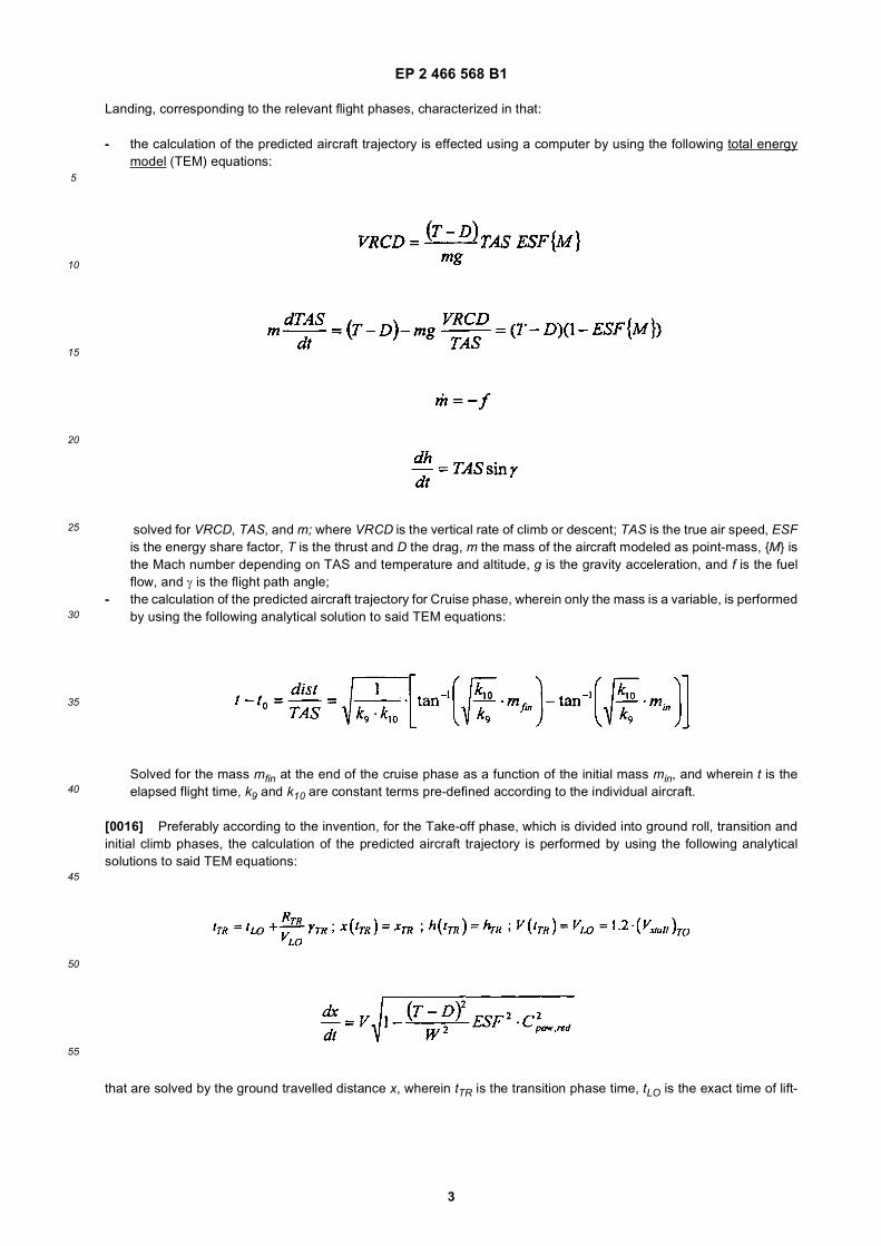
- the calculation of the predicted aircraft trajectory is effected using a computer by using the following total energymodel (TEM) equations:

solved for VRCD, TAS, and m; where VRCD is the vertical rate of climb or descent; TAS is the true air speed, ESFis the energy share factor, T is the thrust and D the drag, m the mass of the aircraft modeled as point-mass, {M} isthe Mach number depending on TAS and temperature and altitude, g is the gravity acceleration, and f is the fuelflow, and γ is the flight path angle;

- the calculation of the predicted aircraft trajectory for Cruise phase, wherein only the mass is a variable, is performedby using the following analytical solution to said TEM equations:

Solved for the mass mfin at the end of the cruise phase as a function of the initial mass min, and wherein t is theelapsed flight time, k9 and k10 are constant terms pre-defined according to the individual aircraft.

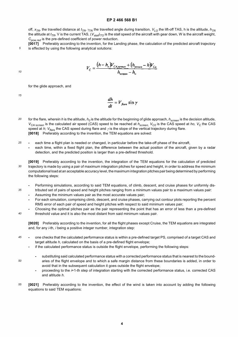
[0016] Preferably according to the invention, for the Take-off phase, which is divided into ground roll, transition andinitial climb phases, the calculation of the predicted aircraft trajectory is performed by using the following analyticalsolutions to said TEM equations:

that are solved by the ground travelled distance x, wherein tTR is the transition phase time, tLO is the exact time of lift-

EP 2 466 568 B1

4

5

10

15

20

25

30

35

40

45

50

55

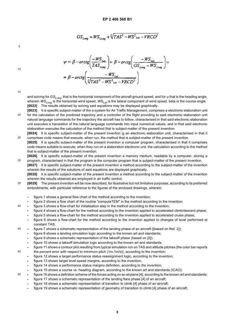
off, xTR, the travelled distance at tTR, γTR the travelled angle during transition, VLO the lift-off TAS, h is the altitude, hTRthe altitude at tTR, V is the current TAS, (Vstall)TO is the stall speed of the aircraft with gear down, W is the aircraft weight,Cpow,red is the pre-defined coefficient of power reduction.[0017] Preferably according to the invention, for the Landing phase, the calculation of the predicted aircraft trajectoryis effected by using the following analytical solutions:

for the glide approach, and

for the flare, wherein h is the altitude, h0 is the altitude for the beginning of glide approach, hscreen is the decision altitude,VCA,screen is the calculated air speed (CAS) speed to be reached at hscreen, VC0 is the CAS speed at ho, VC the CASspeed at h; Vflare the CAS speed during flare and γ is the slope of the vertical trajectory during flare.[0018] Preferably according to the invention, the TEM equations are solved:

- each time a flight plan is needed or changed, in particular before the take-off phase of the aircraft,- each time, within a fixed flight plan, the difference between the actual position of the aircraft, given by a radar

detection, and the predicted position is larger than a pre-defined threshold.

[0019] Preferably according to the invention, the integration of the TEM equations for the calculation of predictedtrajectory is made by using a pair of maximum integration pitches for speed and height, in order to address the minimumcomputational load at an acceptable accuracy level, the maximum integration pitches pair being determined by performingthe following steps:

- Performing simulations, according to said TEM equations, of climb, descent, and cruise phases for uniformly dis-tributed set of pairs of speed and height pitches ranging from a minimum values pair to a maximum values pair:

- Assuming the minimum values pair as the most accurate values pair;- For each simulation, comprising climb, descent, and cruise phases, carrying out contour plots reporting the percent

RMS error of each pair of speed and height pitches with respect to said minimum values pair;- Choosing the optimal pitches pair as the pair representing the point that has an error of less than a pre-defined

threshold value and it is also the most distant from said minimum values pair.

[0020] Preferably according to the invention, for all the flight phases except Cruise, the TEM equations are integratedand, for any i-th, i being a positive integer number, integration step:

- one checks that the calculated performance status is within a pre-defined target PS, comprised of a target CAS andtarget altitude h, calculated on the basis of a pre-defined flight envelope;

- if the calculated performance status is outside the flight envelope, performing the following steps:

- substituting said calculated performance status with a corrected performance status that is nearest to the bound-aries of the flight envelope and to which a safe margin distance from these boundaries is added, in order toavoid that in the subsequent calculation it goes outside the flight envelope;

- proceeding to the i+1-th step of integration starting with the corrected performance status, i.e. corrected CASand altitude h.

[0021] Preferably according to the invention, the effect of the wind is taken into account by adding the followingequations to said TEM equations:

EP 2 466 568 B1

5

5

10

15

20

25

30

35

40

45

50

55

and solving for GSLong, that is the horizontal component of the aircraft ground speed, and for ψ that is the heading angle,wherein WSLong is the horizontal wind speed, WSLat is the lateral component of wind speed, beta is the course angle.[0022] The results obtained by solving said equations may be displayed graphically.[0023] It is specific subject-matter of the a system for Air Traffic Management, comprises a electronic elaboration unitfor the calculation of the predicted trajectory and a controller of the flight providing to said electronic elaboration unitnatural language commands for the trajectory the aircraft has to follow, characterised in that said electronic elaborationunit executes a translation of the natural language commands into input numerical values, and in that said electronicelaboration executes the calculation of the method that is subject-matter of the present invention.[0024] It is specific subject-matter of the present invention is an electronic elaboration unit, characterised in that itcomprises code means that execute, when run, the method that is subject-matter of the present invention.[0025] It is specific subject-matter of the present invention a computer program, characterised in that it comprisescode means suitable to execute, when they run on a elaboration electronic unit, the calculation according to the methodthat is subject-matter of the present invention.[0026] It is specific subject-matter of the present invention a memory medium, readable by a computer, storing aprogram, characterised in that the program is the computer program that is subject-matter of the present invention.[0027] It is specific subject-matter of the present invention a method according to the subject-matter of the inventionwherein the results of the solutions of said equations are displayed graphically.[0028] It is specific subject-matter of the present invention a method according to the subject-matter of the inventionwherein the results obtained are employed in air traffic control.[0029] The present invention will be now described, for illustrative but not limitative purposes, according to its preferredembodiments, with particular reference to the figures of the enclosed drawings, wherein:

- figure 1 shows a general flow chart of the method according to the invention;- figure 2 shows a flow chart of the routine "computeTEM" in the method according to the invention;- figure 3 shows a flow-chart for initialisation step in the method according to the invention;- figure 4 shows a flow-chart for the method according to the invention applied to accelerated climb/descent phase;- figure 5 shows a flow-chart for the method according to the invention applied to accelerated cruise phase;- figure 6 shows a flow-chart for the method according to the invention applied to changes of level performed at

constant TAS;- figure 7 shows a schematic representation of the landing phase of an aircraft ([based on Ref. 2]);- figure 8 shows a landing simulation logic according to the known art and standards;- figure 9 shows a schematic representation of the takeoff phase (based on [2]);- figure 10 shows a takeoff simulation logic according to the known art and standards;- figure 11 shows a contour plot resulting from typical simulation run on TAS and altitude pitches (the color bar reports

the percent error with respect to minimum pitch (1m,1m/s)), according to the invention;- figure 12 shows a target performance status reassignment logic, according to the invention;- figure 13 shows target level speed margins, according to the invention;- figure 14 shows a performance status margins definition, according to the invention;- figure 15 shows a course vs. heading diagram, according to the known art and standards (ICAO);- figure 16 shows a definition scheme of the forces acting on an airplane [4], according to the known art and standards;- figure 17 shows a schematic representation of the landing flare phase [4] of an aircraft;- figure 18 shows a schematic representation of transition to climb [4] phase of an aircraft;- figure 19 shows a schematic representation of geometry of transition to climb [4] phase of an aircraft;

EP 2 466 568 B1

6

5

10

15

20

25

30

35

40

45

50

55

- figure 20 shows a schematic representation of an air traffic control system according to the invention, wherein theflux of information of the present invention is implemented and used.

[0030] The tool according to the invention was developed in the mainframe of SESAR project funded by the EuropeanUnion [5].[0031] The method according to the invention will be also called in the following "Vertical Trajectory Prediction Algorithm"(VTPA). It was developed in order to predict the altitude profile of the trajectory of an aircraft during a typical mission,in the framework of an enhanced-Flight Data Processing (e-FDP) system, i.e. an integrated tool for supporting theactivities of main Air Traffic Management (ATM) European control centers. The above mentioned altimetry profile couldbe combined with geodetic trajectory profile in order to allow for full trajectory prediction.[0032] The main purpose for the realization of the algorithm is to generate a realistic vertical trajectory profile for eachoperating mode that is commanded by Air Traffic Controllers. The list of all implemented operating modes is reportedin the following section.[0033] The vertical trajectory profile was defined by means of a time series of a collection of data that was calledperformance status (PS). This type of information was determined by estimating the following terms for each instant inthe time sequence:

1. Aircraft Mass (m) [tons];2. Estimated Time Over (ETO or t) [10-7s];3. Estimated Level Over (ELO or h) [feet];4. True Air Speed (TAS) [knots];5. Ground Speed (GS) [knots];6. Vertical Rate of Climb or Descent (VRCD or ROCD) [feet/s];7. Travelled distance dtravel [NMi];8. Ground Temperature (GT) [°C];9. Normal acceleration [g];10. Longitudinal acceleration [g];11. Aircraft heading ψ (°).

[0034] Moreover, a solution had to be produced for each type of maneuver that could be commended by Air TrafficControllers during a flight. Some project constraints were assigned to the system so that it would be adequate for real-timeoperation of conflict resolution routines. It must be capable to accurately track the performance status of aircrafts duringall typical transport aircraft flight phases such as takeoff, climb, cruise, descent, and landing. The aircraft dynamics wasdetermined by using the Total Energy Model (TEM) that turned out as an efficient point-mass model [1]. Aircraft config-uration parameters included in the database named Base of Aircraft Data™ (BADA) v.3.1 [1]. This database was realizedby EUROCONTROL™.[0035] Figure 1 reports the main flow-chart of VTPA algorithm.

Main algorithm features

Operating modes

[0036] Several operating modes are provided for the VTPA algorithm, such as:

1. Take Off mode. This mode generates a PS time series for a take-off of an aircraft;2. Landing mode. This mode generates a PS time series for a landing of an aircraft;3. Reach a speed mode. This mode generates a PS time series for a speed and level switch flight segment of anaircraft;4. Reach a level mode. This mode generates a PS time series for a level switch flight segment of an aircraft;5. Keep a state mode. This mode generates a PS time series for a steady cruise flight segment.6. Performance Status Reassignment mode. This mode reassigns the final PS as specified in modes 3 and 4 if,downstream of numerical integration, one determines a PS outside the actual flight envelope.7. Performance status and performance margins modes. These two modes computes the speed and altitude marginsof the actual performance status with respect to the actual flight envelope.

Input parameters

[0037] Initial Performance Status that is composed by the following terms:

EP 2 466 568 B1

7

5

10

15

20

25

30

35

40

45

50

55

1. Initial mass;2. Initial ETO;3. Initial ELO;4. Initial TAS;5. Initial Ground Speed;6. Initial VRCD;7. Initial travelled distance;8. Initial Ground Temperature;9. Initial normal acceleration; 10. Initial longitudinal acceleration; 11. Initial heading.

[0038] Depending on the operating mode, the following terms may be also input:

1. Level to reach - htarget [feet], i.e. the level that must be reached at the end of the mission segment (modes 1-4);2. TAS to reach - TAStarget [knots], i.e. the TAS that must be reached at the end of the mission segment (mode 3);3. Distance to reach - dtarget. This distance is used for KeepAState, i.e. cruise, mode. dtarget is the distance coveredduring the cruise flight segment (mode 5);4. Maximum distance to reach a level dlev [NMi], i.e. the maximum distance that can be travelled before reaching alevel (modes 1-4);5. Maximum distance to reach a TAS dTAS [NMi], i.e. the maximum distance that can be travelled before reachinga stated value of TAS (mode 3);6. Performance modulation. This is a flag. If it is true, then minimum, mean, and maximum thrust configuration shallbe performed in order to reach the constraints. If it is false, only minimum thrust configuration must be performed(modes 1,3,4);7. Aircraft position. It is a data set that contains information about local values of environmental conditions, i.e. sealevel temperature and wind, for given values of travelled distance (all modes).

Output parameters

[0039]

1. Time series of Performance Status;2. Constraint states for final Level and/or TAS:

a. Minimum - if the final value is reached with economic thrust/ESF combination;b. Mean - if the final value is reached with nominal thrust/ESF combination;c. Maximum - if the final value is reached with maximum thrust/ESF combination.

3. Constraint reached indexes, i.e. the array indexes in the PS array where final level/TAS are reached.

External data

[0040] The external data used as aircraft data are taken from database BADA™ that is provided by EUROCONTROL™.It contains both global aircraft information, such as maximum accepted longitudinal acceleration, and single aircraftparameters values, such as wing span. As prior art feature, it is constantly updated to contain parameters of all currentlyflying aircrafts.

Requirements

[0041] This section describes the initial requirements for the method or "tool" according to the invention. The underlyinglogic for requirement definition was driven by a series of issues, such as:

i. Tool routines must be capable to support real-time operation of an ATM management system;ii. The tool must make use of widely used databases of aircraft performances so that it could be easily updatedwhen new aircrafts were introduced in the airspace;iii. The tool must be able to estimate the aircraft performance status for all typical flight phases with adequateaccuracy on all terms;iv. The tool must be able to determine up to three solutions for each call of Reach a Speed, Reach a Level, andTakeoff modes. These solution are tagged as Minimum, Mean, and Maximum and they must be relevant to three

EP 2 466 568 B1

8

5

10

15

20

25

30

35

40

45

50

55

different levels for the values of Thrust and Energy Share Factor (ESF). This latter is defined as the ratio betweenthe energy devoted to climb/descent to the energy needed to keep the level.

TEM software architecture

[0042] The purpose of the tool according to the invention was to determine the aircraft a time series of performancestatuses relevant to a trajectory vertical profile of an aircraft. This calculated time series can be determined once aninitial state and a specific thrust profile was assigned. As reported in the previous section, the main dynamics modelselected was TEM10 that was a point-mass aircraft model represented by the following set of equations:

[0043] Solved for VRCD, TAS, m; VRCD is the vertical rate of climb or descent; TAS is the true air speed, ESF is theenergy share factor, T is the thrust and D the drag, m the mass of the aircraft modeled as point-mass, {M} is the Machnumber that can be calculated as a function of the TAS and temperature, g is the gravity acceleration, f is the fuel flowand γ is the flight path angle.[0044] The term ESF is the energy share factor accounting for aircraft attitude in the airspeed axis reference framethat can be expressed as a function of Mach number {M} [1].[0045] TEM routines are organized according to the invention in a software architecture that is composed by threetypes of routines such as:

1. Routines for pre-processing of aircraft database;2. Runtime trajectory prediction routines;3. Routines for testing results.

[0046] Since BADA database [1] is compiled in ASCII text format, the first type of routines have been developed inorder to make its data available for runtime routines. Moreover, all data that is constant for runtime routines and thatcan be derived from BADA database or from other references was initialized using these routines.[0047] The achievement of the assigned trajectory prediction requirements is carried out by the second type of routines.A main routine implements the general form of the algorithm that supports trajectory prediction services. A series ofsubroutines realize specialized tasks, such as:

1. Initialization of parameters;2. Check of flight envelope constraint violation;3. Realization of trajectory prediction steps, i.e. determination of aerodynamics drag and thrust.

[0048] Finally, a routine for chain testing algorithm performances was developed by the invention. Chain testing wasneeded for the determination of accuracy and to avoid performance regression during debugging.

Preprocessing routines

[0049] Two main database structures have been initialized (imported in the invention method tool) to be used for thetrajectory prediction algorithm:

1. A structure named "BADA" by the invention that contains all and only the data contained in the BADA™ databasedeveloped by EUROCONTROL™. It is divided into three substructures by the same EUROCONTROL™, i.e.:

EP 2 466 568 B1

9

5

10

15

20

25

30

35

40

45

50

55

a. A substructure named "OPF" that contains all data that are relevant to a single particular aircraft. Indeed,"BADA" contains one "OPF" for any aircraft included in the database;b. A substructure named "APF" that contains all data that are relevant to airline procedures for a single aircraft;c. A substructure named "GPF" that contains all constant parameters that are common to all aircrafts.

2. A structure named "TEM" that contains all the data that can be derived from the BADA™ database but that areconstant for the trajectory prediction algorithm. It can be divided into three substructures, such as:

a. A substructure named "conversions" that contains all conversions factors among the different measurementunits adopted in the trajectory prediction algorithm;b. A substructure named "Global" that contains global parameters, such as the maximum allowed TAS in mid-airflight;c. A substructure named "Aircraft" that contains parameters specific to each aircraft.

Runtime trajectory prediction routines

[0050] This section reports flow-charts for all components of VTPA routines. Routine names are highlighted in red infigures. The main routine that performs general form of trajectory prediction routines is called "computeTEM". It isorganized following the scheme reported in Figure 2. The general algorithm is capable to estimate all the terms requiredfor VTPA as above described, such as:

1. Determination of final and partial Performance Status for accelerated climb/descent (Reach a Speed mode);2. Determination of final and partial Performance Status for accelerated cruise (Reach a Speed mode);3. Determination of final and partial Performance Status for constant TAS climb/descent (Reach a Level mode);4. Determination of final ad partial Performance Status for constant TAS cruise (Keep a State mode);5. Determination of final ad partial Performance Status for Take Off (Take Off mode);6. Determination of final ad partial Performance Status for Landing (Landing mode).

[0051] Mode 5 and 6 are needed since the BADA data base does not contain parameters to allow for dynamicsintegration during take-off and landing. For this reason, a pure kinematic model is adopted to carry out PS estimateswhen the aircraft level is below 3000ft with respect to departure/landing runway. This model will be described in thefollowing.

Initialization

[0052] The initialization block has two main purposes:

1. The initialization of parameters used for the integration;2. Performing a check in input values consistency.

[0053] The relevant flow-chart is reported in Figure 3.

Description of TEM Init block

[0054] This block perform the initialization of integration parameters such as mass, TAS, ELO, ETO, dtravel, and VRCD.They are set equal to the input PS unless initial or final TAS is set to 0 (takeoff or landing conditions). In these lattercases, initial and final TAS are set equal to minimum TAS during takeoff or landing, that is derived by BADA™. Whenthis correction is performed, also the initial/final altitude is set to 3000 ft above runway level, i.e. the altitude where takeoffand landing end.

Description of InputCheck block

[0055] The InputCheck routine performs the checks reported in table 1 in order to verify the correctness of inputparameters. The call generates an exception if a single check fails.[0056] Maximum and minimum TAS is determined considering maximum and minimum Calibrated Air Speed (CAS)and Mach reported in BADA by means of the following procedure:1. Given current temperature at sea level, current local temperature, pressure, density, and speed of sound are computedfollowing the ISA atmospheric model [1];

EP 2 466 568 B1

10

5

10

15

20

25

30

35

40

45

50

55

2. Mach and CAS constraints are transformed into TAS constraints;3. Initial condition are verified on initial mass values;4. Final max TAS and ELO are verified for initial mass values;5. Final minimum TAS is verified for minimum operative mass, i.e. the mass that determines the minimum constraint.

Summary of input and output terms for Initialization

Input terms:

[0057]

1. Initial PS;2. Level to reach - htarget [feet], i.e. the level that must be reached at the end of the mission segment (modes 1-4);3. TAS to reach - TAStarget [knots], i.e. the TAS that must be reached at the end of the mission segment (mode 3);4. Distance to reach - dtarget. This distance is used for KeepAState, i.e. cruise, mode. dtarget is the distance (mode 5);5. Maximum distance to reach a level dlev [NMi], i.e. the maximum distance that can be travelled before reaching alevel (modes 1-4);6. Maximum distance to reach a TAS dTAS [NMi], i.e. the maximum distance that can be travelled before reachinga stated value of TAS (mode 3).

Output terms

[0058] The output terms are the same input terms after the following actions are performed:

1. Initial and/or final TAS and/or altitude are corrected if initial/final TAS is equal to 0, i.e. the TAS is set at a minimumvalue that is sufficient for altitude keeping;2. All parameters are verified to stay within reasonable flight constraints.

Table 1

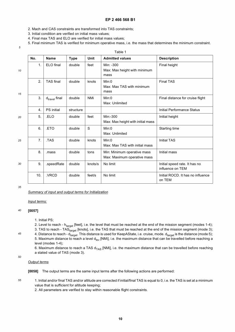
No. Name Type Unit Admitted values Description

1. ELO final double feet Min: -300 Final height

Max: Max height with minimum mass

2. TAS final double knots Min:0 Final TASMax: Max TAS with minimum mass

3. dtravel final double NMi Min:0 Final distance for cruise flightMax: Unlimited

4. PS initial structure Initial Performance Status

5. .ELO double feet Min:-300 Initial heightMax: Max height with initial mass

6. .ETO double S Min:0 Starting timeMax: Unlimited

7. .TAS double knots Min:0 Initial TASMax: Max TAS with initial mass

8. .mass double tons Min: Minimum operative mass Initial massMax: Maximum operative mass

9. .speedRate double knots/s No limit Initial speed rate. It has no influence on TEM

10. .VRCD double feet/s No limit Initial ROCD. It has no influence on TEM

EP 2 466 568 B1

11

5

10

15

20

25

30

35

40

45

50

55

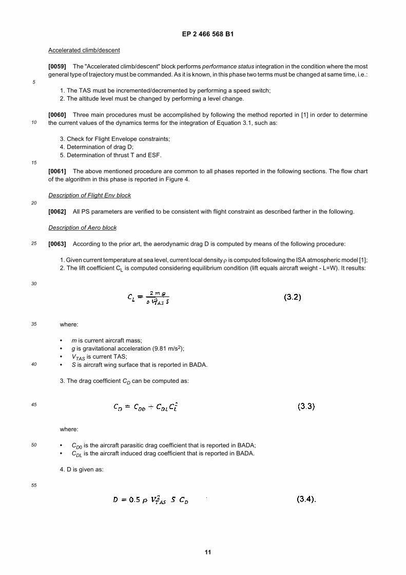
Accelerated climb/descent

[0059] The "Accelerated climb/descent" block performs performance status integration in the condition where the mostgeneral type of trajectory must be commanded. As it is known, in this phase two terms must be changed at same time, i.e.:

1. The TAS must be incremented/decremented by performing a speed switch;2. The altitude level must be changed by performing a level change.

[0060] Three main procedures must be accomplished by following the method reported in [1] in order to determinethe current values of the dynamics terms for the integration of Equation 3.1, such as:

3. Check for Flight Envelope constraints;4. Determination of drag D;5. Determination of thrust T and ESF.

[0061] The above mentioned procedure are common to all phases reported in the following sections. The flow chartof the algorithm in this phase is reported in Figure 4.

Description of Flight Env block

[0062] All PS parameters are verified to be consistent with flight constraint as described farther in the following.

Description of Aero block

[0063] According to the prior art, the aerodynamic drag D is computed by means of the following procedure:

1. Given current temperature at sea level, current local density ρ is computed following the ISA atmospheric model [1];2. The lift coefficient CL is computed considering equilibrium condition (lift equals aircraft weight - L=W). It results:

where:

• m is current aircraft mass;• g is gravitational acceleration (9.81 m/s2);• VTAS is current TAS;• S is aircraft wing surface that is reported in BADA.

3. The drag coefficient CD can be computed as:

where:

• CD0 is the aircraft parasitic drag coefficient that is reported in BADA;• CDL is the aircraft induced drag coefficient that is reported in BADA.

4. D is given as:

EP 2 466 568 B1

12

5

10

15

20

25

30

35

40

45

50

55

Description of Thrust mix block

[0064] Thrust and ESF are computed depending on the selected Performance Modulation following the procedurereported farther in the following.

Summary of input and output terms for Initialization

Input terms:

[0065]

1. Initial PS;2. Level to reach - htarget [feet], i.e. the level that must be reached at the end of the mission segment (modes 1-4);3. TAS to reach - TAStarget [knots], i.e. the TAS that must be reached at the end of the mission segment;4. Maximum distance to reach a level dlev [NMi], i.e. the maximum distance that can be travelled before reaching alevel;5. Maximum distance to reach a TAS dTAS [NMi], i.e. the maximum distance that can be travelled before reachinga stated value of TAS.

Output terms

[0066]

1. Time series of Performance Status;2. Constraint states for final Level and/or TAS:

a. Minimum - if the final value is reached with economic thrust/ESF combination;b. Mean - if the final value is reached with nominal thrust/ESF combination;c. Maximum - if the final value is reached with maximum thrust/ESF combination;

3. Constraint reached indexes, i.e. the indexes in the PS array where final level/TAS are reached.

Accelerated cruise

[0067] In this case, the flight is level (i.e. at constant altitude) but a positive or negative speed switch must be realized.As a consequence, only the speed rate must be determined and VRCD is equal to zero. Figure 5 reports the flow-chartof the algorithm for this phase.

Description of Flight Env2 block

[0068] All PS parameters are verified to be consistent with flight constraint as described above. In this case thealgorithm computational footprint is optimized considering that, being the altitude constant, also all the other parameterswhich depend exclusively on the altitude are constant.

Description of Aero block

[0069] The aerodynamic drag D is computed as above reported.

Description of Thrust mix block

[0070] Thrust is computed depending on the selected Performance Modulation following the procedure reported fartherin the following.

Summary of input and output terms for Initialization

Input terms:

[0071]

EP 2 466 568 B1

13

5

10

15

20

25

30

35

40

45

50

55

1. Initial PS;2. TAS to reach - TAStarget [knots], i.e. the TAS that must be reached at the end of the mission segment;3. Maximum distance to reach a TAS dTAS [NMi], i.e. the maximum distance that can be travelled before reachinga stated value of TAS.

Output terms

[0072]

1. Time series of Performance Status;2. Constraint states for final TAS:

a. Minimum - if the final value is reached with economic thrust level;b. Mean - if the final value is reached with nominal thrust level;c. Maximum - if the final value is reached with maximum thrust level;

3. Constraint reached indexes, i.e. the indexes in the PS array where final TAS is reached.

Constant TAS climb/descent

[0073] This is the case when a level change must be performed without a speed switch. In this case the integrationis performed in order to determine the ROCD. Figure 6 represents the relevant flow-chart.

Description of Flight Env block

[0074] All PS parameters are verified to be consistent with flight constraint as described above.

Description of Aero block

[0075] The aerodynamic drag D is computed as reported above.

Description of Thrust velcost block

[0076] In this case Trust T equals Aerodynamic Drag D (D=T). The resulting T is verified to be less than TMAX.

Summary of input and output terms for Initialization

Input terms:

[0077]

1. Initial PS;2. Level to reach - htarget [feet], i.e. the level that must be reached at the end of the mission segment;3. Maximum distance to reach a level dlev [NMi], i.e. the maximum distance that can be travelled before reaching alevel.

Output terms

[0078]

1. Time series of Performance Status;2. Constraint states for final Level:

a. Minimum - if the final value is reached with economic thrust/ESF combination;b. Mean - if the final value is reached with nominal thrust/ESF combination;c. Maximum - if the final value is reached with maximum thrust/ESF combination;

3. Constraint reached indexes, i.e. the indexes in the PS array where final level is reached.

EP 2 466 568 B1

14

5

10

15

20

25

30

35

40

45

50

55

Constant TAS cruise

[0079] When the aircraft is commanded to perform a constant TAS cruise for a given distance only the current massmust be updated. For the presented application an original analytical solution was developed that allows to determinethe mass change between two cruise segments in a single step. This solution is documented farther in the following.

Takeoff and Landing

[0080] According to Figure 8 [2], a typical landing phase consists of the following sequences:

• Glide approach to the runway, during which the glide path angle, γ, is held constant. In addition, this angle is keptas small as possible (usually between 2.5° and 3°) so to minimize the rate of sink, thus reducing the energy to bedissipated at the impact with the ground;

• Flare to touchdown, during which the speed vector is rotated so to reach a level flight condition at the runway leveland further minimize the rate of sink;

• Ground roll, during which spoilers, brakes, eventually thrust reverse is applied to bring the airplane to the exit speedfrom the runway.

[0081] With reference to the BADA model [1], the initial conditions for landing are specified in terms of both altitudeand Calibrated Air Speed (CAS) as follows (see Figure 8):

[0082] These conditions are the ones computed with the BADA model as the terminal conditions of a descent to 3000ft [1]. At this point, the simulation of the glide approach phase of the landing process is realized by defining a scheduledCAS sequence to bring the airplane at the screen or obstacle height (hobs in the figure) with the correct CAS, as requiredby Federal Aviation Regulations:

[0083] Specifically, the minimum required approach CAS is set at the obstacle height. For the glide approach simulationthe Trajectory Energy Model [1] is used. The glide approach ends when the altitude for flare starting is reached. Theflare altitude is computed within the flare model and it depends on the incremental lift used to curve the flight path, whichin turns depends on the piloting technique.[0084] The terminal conditions of the glide approach are the initial conditions for the simulation of the flare maneuverwhich brings the airplane to have the speed vector parallel to the runway. The flare is reproduced by adopting a modelproposed in [3], which is based on flight data.[0085] For this analysis the ground roll phase is not of interest. The following block diagram summarizes the landingsimulation logic.

Take-off Model Logic

[0086] Following the same approach of the landing, the overall takeoff process can be broke down in three phases(see Figure 9):

• Ground Roll, during which the airplane is accelerated until the liftoff speed is reached;

EP 2 466 568 B1

15

5

10

15

20

25

30

35

40

45

50

55

• Transition to Climb, during which the flight path angle varies gradually from zero (at liftoff) to a constant value forclimb;

• Initial Climb, during which the airplane follows the takeoff flight path until a safe height above the terrain is reachedand climb to-cruise altitude is started.

[0087] In this analysis only the second and third phases are of interest since the simulation will be started from theliftoff condition. Thus, the initial values of the state parameters are the ones specified at the end of the ground roll phase:

where hrwy is the runway altitude above sea level. We propose to employ a different model for each of the above phases,separately described in the following. Figure 10 summarizes the takeoff simulation logic. The simulation is started fromthe liftoff condition which determines the initial conditions for the transition to climb phase, during which the airplaneflight path curves until the flight path angle of the initial climb condition is reached. This last one depends on the incrementallift used to curve the trajectory and on the maximum thrust amount used to climb out. To simulate this phase a modelwhich integrates the climb model and the acceleration limits proposed in BADA with the piloting technique and the modelfor transition proposed in [3] has been developed. Once the terminal condition of transition is reached the climb phaseis started by the scheduled CAS sequence suggested by the BADA model. Climb is terminated when the airplane reaches3000 ft.

Description of technical issue that has been solved by the solution according to the invention.

[0088] The proposed method tool is intended to provide real-time trajectory prediction capabilities at average levelaccuracy to systems for the automation of Air Traffic Management function. These tools will provide autonomous reso-lution of potential future conflicts during flight. The main original issues that were not available before this tool wasdeveloped are reported in the following list:

1. Real time capability to predict in a few seconds the altimetry trajectories of all aircraft flying over an extendedregion under ATC control;2. The tool supports multi-mode execution of maneuvers, when applicable. Indeed, nominal mode, maximum thrustmode, and economic mode have been implemented in the case of change of level and/or speed switch;3. The tool is capable to check if a developing trajectory can be actually flown by the aircraft. Indeed, flight envelopeconstraint are verified in real-time during integration;4. The tool includes the capability to simulate a complete mission including terminal phases, such as landing andtakeoff;5. To prevent failure in reaching a flight state or level, the tool is capable of computing in real-time the speed andaltitude margins for any flight state and atmosphere condition with respect to the actual flight envelope. Estimatedmargins can be used to drive the trajectory prediction process;6. In case a failure notice is generated, because an algorithm call requires speed values or final height outside theenvelope, the tool outputs indications in order to address a new call to the nearest status that can be accomplishedwith successful compliance of the envelope limits.

[0089] In the following subsections the main original issues of the presented tool are reported.

Analytical solution for determining the final mass after a cruise flight segment

[0090] In order to minimize the number of computations, an original analytical solution was developed so that a preciseestimate of the aircraft mass variation could be carried out after a cruise flight segment of any size. In the case of steadycruise, the single term that changes in the performance status is the mass for flight segment contained in a region withconstant temperature, pressure, and wind. The solution that has been carried out allowed for avoiding any form of timeconsuming numerical integration. When intermediate estimate are needed the solution can be applied to segments withreduced size.[0091] First of all, the lift coefficient CL is determined for steady cruise when lift equals aircraft weight:

EP 2 466 568 B1

16

5

10

15

20

25

30

35

40

45

50

55

[0092] Subsequently, the drag coefficient CDis derived by means of the polar equation:

[0093] Where CD0 is the parasitic drag coefficient and CDt is the induced drag coefficient. These terms can be derivedby BADA™ database. The constant terms ki can be easily deduced. Thus, the drag D can be determined as follows:

[0094] Where ρ is the local density and S is the aircraft reference wing surface (from BADA). In steady cruise thrustequals drug:

[0095] Since the time derivative of the aircraft mass m equals the opposite of the fuel flow f, i.e. a linear term of T, thefollowing non linear differential equation can be written;

[0096] Equation (6.5) can be rearranged as follows by extracting the differential terms:

[0097] Moreover, all terms depending on mass can be put on the left side of the equation:

[0098] The expression of m reported in equation (6.7) can be replaced by the one in equation (6.5):

·

·

EP 2 466 568 B1

17

5

10

15

20

25

30

35

40

45

50

55

[0099] The resulting integral problem is given in the following equation:

[0100] Equation (6.9) can be integrated in order to carry out the analytical expression of the mass at the end of thecruise segment mfin as a function of the initial mass min:

[0101] This equation can be solved with inference on trigonometric terms and is independent from the type of engineof the aircraft.

Control by selection of proper Thrust and ESF mix

[0102] The control terms in equation (3.1) are:

1. The aircraft thrust T;2. The aircraft Energy Share Factor ESF.

[0103] In order to emulate the pilot’s behavior after a command is sent from ATC, a proper arrangement of the abovereported terms must be selected. The values derived by the invention to this extent are reported in table 6.1.

Table 6.1

Commanded maneuver

Commanded speed switch

Commanded mode Thrust ESF

Climb Increase Economic Cpower red*Tmax, climb Const CAS ESF (sec. 3.2 of [1])

Average Cpower red*Tmax, climb 0.3

Max climb angle Tmax, climb 0.3

Decrease Economic Tidle 1.7

Average Cpower red*Tmax, climb 1.7

Max climb angle Tmax, climb 1.7

Descent Increase Economic Tdes 1.1

Average Tdes 1.4

Max descent angle Tdes 1.7

Decrease Economic Tdes 0.7

Average Tdes 0.5

Max descent angle Tdes 0.3

Cruise Accelerated Cpower red*Tmax, climb 0

Constant speed D 0

Decelerated Tdes 0

EP 2 466 568 B1

18

5

10

15

20

25

30

35

40

45

50

55

[0104] Indeed, four modes were adopted for thrust T, such as:

1) Maximum Climb Thrust (Tmax, climb). It is a thrust level that could be sustained only for a short time by engines.Typically, it is used for initial climb during takeoff. It is the continuous maximum thrust limit reported in aircraft manual(sec. 3.7.1 of [1]);2) Reduced Climb Power. In order to avoid engine wear and excess fuel consumption, standard climbs are realizedwith a reduced power consumption correction factor (Cpower red) as reported in sec. 3.8 of [1];3) Maximum Cruise Thrust (Tmax, cruise). It is the maximum thrust allowed during cruise phase (sec. 3.7.2 of [1]);4) Descent Thrust (Tdes). It depends on altitude and flight phase (sec. 3.7.3 of [1]).

[0105] All thrust laws depend on Tmax, c/imb. It is a function of engine type, h, VTAS, and temperature.[0106] In order to simulate pilot behavior, a proper control was introduced on longitudinal acceleration so that T isproperly reduced to avoid constraint infringement of aforesaid parameter. Indeed, also human and automatic pilotsperform the same control during real flights to keep the aircraft within acceleration safety boundaries.

Minimization of the computational load

[0107] Each phase reported above with reference to Figure 1 has been coded so that the number of computations isoptimized for the specific application. Therefore, when TAS or level is constant all terms that are constant with TAS orlevel have been computed only during initialization. Moreover, during steady cruise flight the single step analytical solutiondescribed above was applied. A test with specific benchmarking tools [12] reported a reduction of more than 30% in themean computational load.

Check of Flight Envelope constraint

[0108] Flight envelope is defined on the basis of the BADA™ database. One performs a check of position inside theenvelope for the initial state and at every integration step.. Also temperature effect was accounted for. Indeed, temperaturevariations from standard atmosphere model up to 10° C could produce an error up to 10% in the determination of d.This effect had an important impact on turbojet aircraft trajectory prediction performances. For the definition of the flightenvelope within the TEM model seven types of constraint on status are provided:

1) Maximum CAS VMO that accounts for maximum Lift and Drag levels;2) Maximum Mach number MMO that accounts for effects of air compressibility;3) Maximum altitude hmax/act for a given aircraft mass m and temperature T;4) Minimum CAS Vmin that is determined by stall;5) Buffet Mach number Mb that is a limit due to vibrations induced in jet engines;6) Maximum longitudinal acceleration acclong max that is determined by flight regulations;7) Maximum normal acceleration accnorm max that is determined by flight regulations.

[0109] Constraints (1-5) were Flight Envelope constraints depending on aircraft type and flight status, whereas con-straints 6 and 7 were global aircraft constraints.

Inclusion of Takeoff and Landing by means of kinematic models

[0110] The aircraft data included in the BADA™ data base does not allow for direct dynamical integration of aircraftvertical trajectory for flight phases below 3000 ft. In particular, this is due to a not negligible modification of standardmodels of drag and thrust in these phases. Indeed, aerodynamic drag must account for ground effect while thrust hasspecific issues that cannot be derived from the analysis of radar tracks during cruise, i.e. the way BADA database iscompiled.[0111] The model proposed by the present invention is based on a dynamical inversion of TEM equations (3.1). Theaircraft vertical trajectory is assumed to be equal to the one reported by ICAO in its regulations. The dynamical terms,i.e. drag and thrust, are derived in each segment of takeoff and landing phases as reported farther in the following(explanations leading to equations A) together with a description of the implemented routines.

Determination of integration pitch

[0112] Another important aspect that was taken into account was the selection of pitch for time integration. Becauseof the calls to the various services, the distance travelled by the airplane can be remarkable, an integration strategy with

EP 2 466 568 B1

19

5

10

15

20

25

30

35

40

45

50

55

variable pitch has been chosen, namely the maximum values of integration pitch were assigned considering maximumallowed altitude and true air speed variations.[0113] A proper procedure was selected to estimate the values of maximum integration pitches to address the minimumcomputational load at an acceptable accuracy level. Simulations used to test climb, descent, and cruise phases whererepeated for uniformly distributed pairs of speed and height pitches ranging from minimum (1m,1m/s) to (300m,100m/s).For each run, contour plots similar to the one reported in figure 11 were carried out. They reported the percent error ofeach pair of speed and height pitches with respect to the pair (1m,1m/s) that was estimated to be the most accurate.The optimal pitches were selected considering the criterion that they should represent the point that had an error of lessthan 1% and it was also the most distant from (1m,1m/s). Such an analysis produced the choice of the integration pitches(40m,25m/s). Figure 3 reports the results of tests of 151 climb conditions compared to the ones output by BADA Tools™developed by EUROCONTROL™. It is worth noting that the mean error was in the order of 0.1 % and rms error changedslightly from 9% to 10% whereas the total number of computations was critically reduced. Pitch selection had no effecton cruise at constant speed, since the tool was capable to compute the aircraft mass at the end of cruise segment in asingle computational step.

Performance Status Reassignment

[0114] Another important aspect that was taken into account was the possibility of reassigning the target performancestatus in case it lies outside the flight envelope. Indeed, some implemented modes require the aircraft reaches a targetlevel (reach a level) or target speed and level (reach a speed). In this cases, it is not enough to check that the targetperformance status lies within the initial flight envelope, since it may move outside the actual flight envelope during theintegration process. To overcome this problem specific methods have been developed and implemented in order tocheck for target performance status inclusion in the actual flight envelope and reassign it in case it lies outside the actualflight envelope, which is affected by actual mass and atmospheric conditions.[0115] Let suppose that a target performance status has been assigned:

[0116] Starting from an initial performance status, given initial mass M0 and temperature at sea level, Tsl, we caneasily check for target performance status inclusion in the flight envelope corresponding to the initial mass and temper-ature at sea level (blue boundary in Figure 12). In the following, for the sake of brevity, we consider only the effect ofthe aircraft mass.[0117] Let suppose that at the i-th integration step, at which the airplane mass is reduced from M0 to Mi, the maximumspeed boundary of the flight envelope moves to the left (red boundary in figure 12) leaving the target performance statusnow outside the actual flight envelope. The target performance status becomes now unfeasible, and needs to be reas-signed.[0118] The implemented logic relies on computing the nearest target performance status on the red boundary andthen shifting the target performance status to the point on the black boundary (XTN) computed by applying a safe marginto the nearest target status. This procedure is repeated each time the target performance status moves outside theactual flight envelope and the safe margin is computed so to reduce the number of times the procedure is applied.However, it is sufficiently small so to keep small the difference between the reassigned target status and the original one.[0119] The implemented procedure provides also an estimate of the speed derivative with respect to altitude evaluatedas the inverse of the slope of the line connecting the actual performance status to the target one. Indeed, this quantitycan be used in the choice of the most appropriate energy share factor, i.e. the most appropriate aircraft attitude, to reachthe desired performance status.[0120] In case only a target level is specified (reach a level mode), the above procedure concerning the calculationsof the margins with respect to the flight envelope allows computing the admissible speed range corresponding to thattarget flight level on the actual flight envelope (see Figure 13). This information can be used to drive the integrationprocess toward the target altitude without violating the flight envelope in terms of speed. In addition, the procedureprovides also the speed derivative with respect to altitude evaluated as the inverse of the slope of the lines connectingthe actual performance status, Xi, to the points corresponding to the minimum and maximum admissible speeds at thetarget altitude. These values provides a range of admissible slopes that can be used to shape the Energy Share Factorused to reach the target altitude.

EP 2 466 568 B1

20

5

10

15

20

25

30

35

40

45

50

55

Performance Status margins

[0121] Another implemented innovative solution concerns the computation of the actual performance status margins(speed and altitude) with respect to the actual flight envelope boundary. The margins are defined as in Figure 14. Theknowledge of the actual values of these margins allows properly driving the integration process, in terms of time, speedand/or altitude variations, to avoid that the actual performance status moves outside the flight envelope, which can causea failure in the integration process.

Evaluation of wind effect

[0122] The developed method tool can estimate the effect of wind on aircraft performance status. This effect is givenby estimating the following terms:

1. Aircraft ground speed (GS) as a function of true air speed (TAS) and wind speed (WS);2. Aircraft heading ψ as a function of course angle β, TAS, and WS.

[0123] For the first term the following method has been carried out. The demonstration needs that the Aircraft Ground-speed Reference Frame (AGRF) is defined. It is the frame that has x axis alongside current groundspeed direction, yaxis in the horizontal plane and normal to x axis, z axis alongside vertical direction. It results that x axis is tangent toaircraft ground trajectory, i.e. longitudinal axis, whereas y axis is normal to aircraft ground trajectory, i.e. lateral axis. LetWS have the following components in the AGRF frame:

[0124] These components are given from meteo information in each point of the aircraft trajectory. It is worth notingthat the vertical wind speed is non negligible only for short term not stationary events such as wind gusts and windshares. Moreover, it is not reported in meteo information.[0125] In the same reference frame, GS is given as:

while aircraft TAS=GS-WS can be estimate as:

[0126] Since VRCD and the norm of TAS are estimated by means of integration of TEM equations (3.1), the determi-nation of GS is completed once GSLong is computed. The square of the norm of TAS can be derived from (6.13):

EP 2 466 568 B1

21

5

10

15

20

25

30

35

40

45

50

55

[0127] Equation (6.14) is a quadratic equation in GSLong that admits the following solutions:

[0128] Since GSLong must be positive for aircrafts, the negative sign before the square root in equation (6.15) mustbe discarded. As a consequence, the resulting value of GSLong is:

[0129] The aircraft heading ψ, i.e. the angle between the north direction and the aircraft longitudinal axis, can bedetermined once the course angle β , i.e. the angle between the north direction and the horizontal ground speed direction,is given. The method to extract ψ is reported in Figure 15. It results:

Applications that can be improved by using the proposed invention

[0130] The following applications can make use of the developed algorithm:

1. Flight Data Processing software for Air Traffic Management applications. In this case, the algorithm can be usedto predict vertical motion and performance status of all aircrafts in a controlled region in order to perform conflictdetection and resolution. The algorithm can be used for both strategic planning and real-time tactical re-planning;2. Air Traffic Simulation tools for professional and gaming applications. Professional applications include testing ofinnovative flight procedures, e.g. continuous descent flight. The algorithm can be used for real-time simulations ofaircraft behavior after a specific command is issued from a controller. The tool can be installed into Flight ControllersTraining Units, i.e. the units that are used to train Flight Controllers with Synthetic Air Traffic Conditions. In this case,the tool can estimate aircrafts response to Controllers’ commands;3. The tool can be used by innovative onboard avionic instruments, such as next generation Traffic Collision Avoid-ance Systems or a Bad Weather Avoidance System. In this case, it can be adopted to simulate aircraft behavior ifa proper automatic command is issued to avoid dangerous conditions.

Takeoff and landing models

Landing Model Equations

[0131] In the following it is assumed that:

EP 2 466 568 B1

22

5

10

15

20

25

30

35

40

45

50

55

• The airplane moves only in the longitudinal plane• The airplane is in complete trim, i.e. no net pitching, rolling and yawing moments exist.

[0132] Thus the only allowed accelerations are the ones along and perpendicular to the flight path. Under theseassumptions, with reference to Figure 16 [4], the equations of motion of the airplane projected along and perpendicularlyto the flight path are :

[0133] Wherein V is the true air speed, γ is the flight path angle, L is the lift, D is the drag, T is the thrust, W the weightand g the gravity acceleration. If the thrust angle, ΦT, and the angle of attack, α, are assumed small (as typical), the twoequations rewrite as:

[0134] The airplane altitude with respect to the runway and ground range can be then computed by the followingkinematic relations:

where Vg is the ground speed evaluated as the sum of the true air speed and the wind speed:

[0135] In the following, V indicates the True Air Speed (TAS) and VC indicates the Calibrated Air Speed (CAS).

Glide Approach

[0136] During the approach, the airplane is flown along a straight line flight path [4] with an approach speed whichmust satisfy the following CAS constraint until the airplane reaches the obstacle height (50 ft for both 23 and 25 FederalAviation Regulations, FAR):

EP 2 466 568 B1

23

5

10

15

20

25

30

35

40

45

50

55

where Vst,AP is the stalling speed in approach. During the final approach the airplane must be configured to the landingconfiguration, i.e. gear down and flaps in the landing position. Differently from the approach speed, the touchdown speedis not specified by FAR’s, but it is typically approximated as [4]:

[0137] By multiplying the first of equations (A.2) by V and using the first of equation (A.3) we have:

[0138] This equation is the one provided also in the TEM model [2], and it can be used to model the airplane motionfrom the initial altitude, ho, and CAS speed, VCo, to the altitude and speed at the flare starting. Specifically, since in theapproach phase the CAS is constrained to be higher than a minimum (see eq. A.5), a CAS schedule is imposed fromthe initial CAS speed at the initial height so to have the minimum required approach speed at the screen height:

[0139] This CAS schedule is converted into a TAS schedule by using the CAS to TAS conversion formulas providedin the TEM model [3].[0140] Since the flight path angle is kept constant during descent, this additional condition determines that both CASand ROCD (Rate of Climb/Descent) are controlled during approach. As a consequence, equation (A.7) can be used toevaluate the required thrust as follows:

[0141] Of course, it must be controlled that this thrust is not lower than the idle thrust and not higher than the landingthrust as provided in the TEM model [3], i.e the following condition must be satisfied:

where the thrust in landing is evaluated as follows [3]:

[0142] In equation (A.11), Tmax,climb is the maximum thrust in climb provided for the different airplanes in the TEMmodel and CTdes,Id is the thrust correction factor for the landing phase [3].[0143] Once speed, flight path angle and thrust have been evaluated, the airplane altitude and ground range can becomputed by integrating the two kinematic equations (A.3). In addition, the nominal fuel flow, fnom, can be evaluated

EP 2 466 568 B1

24

5

10

15

20

25

30

35

40

45

50

55

according to the formulas reported in the TEM model for the different airplanes [3], thus the fuel consumption can becomputed as a function of time as:

and the airplane mass is determined as:

Where mo is the initial airplane mass.[0144] Finally, the longitudinal deceleration during approach can be easily computed from the variation imposed onthe TAS. Of course, since the flight trajectory is a straight line, the acceleration perpendicular to it is zero.

Flare

[0145] The flare maneuver is modeled as in [4]: the flight path is a curved line, normally assumed to be circular (seeFig. 17) . During the flare the airplane decelerates to the touchdown speed. Thus, an average flare speed can be definedand used to compute the flare parameters:

[0146] During flare the lift must balance the airplane weight and the centrifugal force produced by the curved flightpath, i. e. we have:

where is the atmospheric density, S the wing surface and Rflare is the flare radius. Let we take:

where Vflare1 is the flare speed under unitary lift coefficient. From (A.15) and (A.16), the lift coefficient during the landingflare can be computed as:

where ΔCLflare is the lift coefficient increment needed to curve the airplane trajectory given by:

EP 2 466 568 B1

25

5

10

15

20

25

30

35

40

45

50

55

[0147] The change in the lift coefficient is assumed to be instantaneous [4]. Thus we have:

since:

[0148] Finally, the lift during flare is given as:

[0149] The flare radius can be computed from eq. (18):

wherein nflare is the load factor during flare. It depends on pilot technique, and it is usually between 1.04 and 1.08 [4].Once the flare radius has been computed, with reference to Figure 7, the flare height as a function of γ can be determinedas:

with γ being θflare in Figure 17. The ground range is instead determined as a function of time as follows:

EP 2 466 568 B1

26

5

10

15

20

25

30

35

40

45

50

55

where the flare time can be estimated as

and the ground speed is give as

being Vw the wind speed parallel to the ground.[0150] From equation (22), the lift coefficient increment can be computed as:

and the lift coefficient during flare as:

[0151] Then, the drag coefficient during flare can be computed using the formulation provided in the TEM model [3]:

[0152] The drag force is thus computed as:

[0153] Also the flare angular velocity can be computed as:

[0154] The longitudinal deceleration during flare can be computed by using eq.(A.7) as:

EP 2 466 568 B1

27

5

10

15

20

25

30

35

40

45

50

55

while the acceleration perpendicular to the flight path is given as:

[0155] Finally, the ROCD is evaluated as:

Transition to Climb Phase

[0156] The transition is defined as the phase in which the flight path angle γ goes from 0 (value at the end of the groundroll) to its constant value of the initial climb phase. The transition phase is modeled according to the geometry in Figure18 [4].[0157] The flight path is assumed to be circular, and the velocity is assumed to be constant, i.e. V = VLO. Thus, thetransition phase mainly consists of a rotation of the TAS from being parallel to the runway to being inclined at the initialclimb flight path angle.[0158] As in the flare maneuver, the lift shall balance the airplane weight and produce the centripetal accelerationneeded to curve the trajectory:

[0159] This additional lift is the effect of an excess in the lift coefficient beyond the 1-g one, ΔCL, which produces thecentripetal acceleration given as:

In which is the liftoff speed under unitary lift coefficient.[0160] Ref. 3 suggests employing the following equation for computing ΔCL derived from operational data:

[0161] Assuming, as usual, that lift-off occurs at 120% of stall speed, we have the following expression for Δ CL:

Where

EP 2 466 568 B1

28

5

10

15

20

25

30

35

40

45

50

55

[0162] Thus, the radius of curvature during the transition phase can be computed as:

and the lift coefficient is given by:

whereas the drag coefficient is evaluated as a function of the lift coefficient using the TEM model [3].[0163] The increment in ground range, x, and in altitude, h, during the transition phase can then be computed by thetransition geometry (see Figure 19). The transition is modeled with respect to the air mass, thus the horizontal windeffect shall be added into the x equation. The x, h equations are thus:

Where

[0164] In setting the transition maneuver, it must be checked that the acceleration perpendicular to the flight path islower than the allowed maximum provided in the TEM model [3]. Thus, we have:

[0165] This condition translates into an allowed minimum value for the transition arc radius:

EP 2 466 568 B1

29

5

10

15

20

25

30

35

40

45

50

55

[0166] Finally, using eq. (41) a maximum allowed value for the lift coefficient increment can be found as follows:

[0167] Of course the longitudinal acceleration is zero.[0168] Initial conditions for the transition model are equal to the ground roll phase’s final condition, i.e. t0 = tLO. Theinitial air relative velocity becomes equal to the lift-off velocity (see eq. A.35).[0169] The final conditions for the transition phase are obtained by imposing that the flight path angle is equal to theone for the initial climb, γTR. From TEM model [3] in climb the following expression can be used to evaluate the ROCD:

[0170] Where the power reduction coefficient is introduced to allow the simulation of climbs using less than the maximumclimb setting, and is given by:

[0171] The Energy Share Factor (ESF) is a measure of how much thrust is used to gain altitude with respect to gainingspeed [3]. We assume that during transition the whole thrust is used to gain altitude, which means that ESF ≈ 1.[0172] Thus the ROCD becomes:

from which the climb angle at the end of transition can be derived as:

since:

EP 2 466 568 B1

30

5

10

15

20

25

30

35

40

45

50

55

[0173] The final air relative velocity will still be equal to the lift-off velocity. The transition will take a time tTR, given byinversion of Eq.(A.44) with γ(t) = γTR. The altitude and the position along the runway centerline will be given by Equations(A.42), (A.43):

[0174] As for landing, the fuel consumption is evaluated by using the TEM model for climb [3]. The airplane massvariation is then computed using eq. (A. 13).

Initial Climb Phase

[0175] The initial climb phase starts when the climb angle reaches the value at the transition end and terminates at3000ft. Thus the initial condition for initial climb are defined as:

[0176] In the present invention, the Total Energy Model (TEM) from BADA [3] is employed to describe the aircrafttrajectory in the initial climb phase. In addition, we assume the CAS schedule as given by the TEM model for the differentairplane categories. As an example for jet airplanes we assume the following CAS increment below 3000ft:

[0177] With the above CAS, one can obtain the TAS by employing standard equations (e.g. in [3]).[0178] The TAS schedule from the initial altitude to the final altitude (3000ft) can be then expressed as follows:

[0179] The ground speed can be computed as:

EP 2 466 568 B1

31

5

10

15

20

25

30

35

40

45

50

55

[0180] Once the TAS is available, one can compute the altitude profile by means of the TEM model [3], using thefollowing equation:

where ESF is the Energy Share Factor. BADA suggests to employ ESF=0.3 as the energy share factor value for climbphases [3]. However, preliminary numerical analysis of the capability of the model to predict realistic climb rates suggeststhat a more realistic estimate of ESF is given by [4]:

Where

[0181] Nevertheless, to ensure the continuity between the transition and initial climb phases, the ESF is evaluated byimposing the following condition:

[0182] This translates into the following equations for ESF:

[0183] Lift and Drag are evaluated as:

EP 2 466 568 B1

32

5

10

15

20

25

30

35

40

45

50

55

[0184] The flown range is then obtained by:

And γ is found by the height rate equation:

[0185] Thus:

[0186] The altitude is evaluated using eq. (A.58), whereas the consumed propellant and the mass variation are eval-uated by using the TEM model for climb [3] and eq. (A.13). The longitudinal acceleration is computed from the speedschedule, whereas the normal acceleration is zero due to the straight flight path.[0187] In the prior art, the trajectory prediction is certainly performed, but using a coarse-grained algorithm that makesuse of a tabular database about the aircraft features.[0188] Moreover, there is in the prior art a starting model for using the Eurocontrol databases. This model allows forcalculations of only certain flight phases, and is therefore very limited.[0189] The present invention adds calculation steps which were lacking in the prior art.[0190] In the prior art, only the 2D trajectory is calculated, the altitude and the time are derived.[0191] In the present invention one has:

- Adapted the equations to the commands of the controller;- Provided an equation system and models that allow the rapid calculation with high accuracy, by considering the

mass as variable.

[0192] The commands to be controlled at ground are those relevant to performing a series of codified maneuvers.[0193] The commands in the present invention are at first in the form of words. Then they are translated into numericalinputs to a set of equations. This translation is a novelty feature of the method according to the invention, and takes theplace of the statistics tables currently used.[0194] Since the methods of the present invention allow for the managing of a dynamic situation, one can also imposeconstraints on the whole travel.[0195] The equations modified according to the present invention gives a numerical output.[0196] The old tables described the aircraft behavior by using linearization parameters. For example during a phase,a table gave the travelled length and the relevant travel time.

EP 2 466 568 B1

33

5

10

15

20

25

30

35

40

45

50

55

[0197] In the method according to the invention, there is a constant level of accuracy among the calculated parameters.On the contrary, in the prior art the least accuracy was chosen as reference.[0198] In the prior art: first there is a predicted trajectory, then the controller makes its plannings and proceeds topossible modifications of the predicted trajectory. If during the actual flight there are "tactical" modifications of the con-straints, one proceeds to recalculation of the trajectory. In the method according to the invention, the procedure is thesame but the calculation is made according to the above specification.[0199] In the case of a command that cannot be followed by the aircraft, the method according to the present inventioncalculates the closest performable solution.[0200] Further, the method of the present invention uses different modeling for each phase of take-off and landing.From the regulation constraints, one has understood the effects on the particular aircraft, whilst in the prior art all theaircraft are equally treated.[0201] The present invention gives a break-even solution between the calculations based only on tables and a completeset of differential equations, which would require huge computation resources.[0202] In the integration of equations, according to the invention, one chooses an optimum integration pitch for thewhole integration, whilst in the prior art iterations were used, thus slowing down the calculation.[0203] The present invention may be implemented in a hardware environment, according to figure 20 which show anair traffic control system according to the invention.[0204] The flux of data are represented by continuous lines, whereas the flux of commands are represented withdashed lines. The dotted larger boxe comprises the flight data processor with relevant code (TEM) or memory area(flight plan data, airborne performance database with data relevant to aircraft dimensions, tank capacity etc.) blocks.[0205] Meteo data are taken form an external data service via http or other network protocol, namely form the AutomatedWeather Observing System (AWOS) and Automatic Terminal Information Service (ATIS).[0206] The actual airborne position is taken from the radar, and is utilized to trigger a re-calculation of the predictedtrajectory by TEM equations, in particular for the following cases:

- each time a flight plan is needed or changed, in particular before the take-off phase of the aircraft,- each time, within a fixed flight plan, the difference between the actual position of the aircraft, given by a radar

detection, and the predicted position is larger than a pre-defined threshold.

[0207] From the controller console commands corresponding to the trajectory calculation in the various trajectoryphases are sent to the flight data processor which creates a flight plan and calculate TEM equations on the basis of allthe other parameters it receives from the various hardware and networks. The flight plan, in particular is created uponreception of command from the Automated Fixed Telecommunication Network (AFTN) or other Entity or Institution.[0208] Once the trajectory is calculated, it is sent to the operator console and displayed on the display of the operatormonitoring the situation of the aircraft and air traffic.

References

[0209]

[1] Nuic, A., User Manual for the Base of Aircraft Data (BADA) - Revision 3.6, EUROCONTROL, EEC Note No.10/04, July 2004.[2] Pamadi, B.N., Performance, Stability, Dynamics, and Control of Airplanes, Second Edition, American Instituteof Aeronautics and Astronautics, Reston VA, 2004.[3] Roskam, J, Chan-Tau, E. L., "Airplane Aerodynamics and Performance", 1997.[2] SESAR Consortium, Work Programme for 2008-2013, Doc. SESAR Consortium No. DLM-0710-002-01-00,Bruxelles, Belgium, April 2008.[4] Joint Planning and Development Office, Concept of Operations for the Next Generation Air Transporation System,v.2.0, June 2007.[5] Cistone, J., "Next Century Aerospace Traffic Management: The Sky is No Longer the Limit," AIAA Journal ofAircraft, Vol. 41, No.1, 2004, pp. 36-42.[6] Wu, S.F. and Guo, S.F., "Optimum Flight Trajectory Guidance Based on Total Energy Control of Aircraft," AIAAJournal of Guidance, Control, and Dynamics, Vol. 17, No.2, 1994, pp. 291-296.[7] Slattery, R. and Zhao, Y., "Trajectory Synthesis for Air Traffic Automation," AIAA Journal of Guidance, Control,and Dynamics, Vol. 20, No.2, 1997, pp. 232-238.[8] Dupuy, M.D. and Porretta, M., "Preliminary results for a robust trajectory prediction method using advanced flightdata," IEEE/AIAA 26th Digital Avionics Systems Conference, IEEE, Dallas, TX, 2007, pp. 1.C.5-1-1.C.5-9.[9] Gallo, E., Lopez-Leones, J., Vilaplana, M.A.E., Navarro, F.A., and Nuic, A.," Trajectory computation Infrastructure

EP 2 466 568 B1

34

5

10

15

20

25

30

35

40

45

50

55

based on BADA Aircraft Performance Model," IEEE/AIAA 26th Digital Avionics Systems Conference, IEEE, Dallas,TX, 2007, pp. 1.C.4-1-1.C.4-13.[10] Mondoloni, S., "Development Of Key Performance Indicators for Trajectory Prediction Accuracy," IEEE/AIAA26th Digital Avionics Systems Conference, IEEE, Indianapolis, IN, 2006, pp. 1-11.[11] Nuic, A., Poinsot, C., lagaru, M-G., Gallo, E., Navarro, F.A., and Querejeta, C., "Advanced Aircraft PerformanceModeling for ATM: Enhancements to the Bada Model," IEEE/AIAA 25th Digital Avionics Systems Conference, IEEE,Washington, DC, 2005, pp. 1-12.[12] Minka, T., "The Lightspeed Matlab Toolbox", v.1.3, Microsoft Inc.,2006, available at URL: http://research.mi-crosoft.com/~minka/software/lightspeed/.

[0210] The present invention has been described for illustrative but not limitative purposes, according to its preferredembodiments, but it is to be understood that modifications and/or changes can be introduced by those skilled in the artwithout departing from the relevant scope as defined in the enclosed claims.

Claims

1. A computer-implemented method for the prediction of aircrafts vertical trajectory, in particular for Air Traffic Man-agement, comprising the following flight calculation modules: Take-off; Climb; Cruise; Descent; and Landing, cor-responding to the relevant flight phases, characterized in that:

- the calculation of the predicted aircraft trajectory is effected by a computer processor using the following TotalEnergy Model (TEM) equations:

solving said equations for VRCD, TAS, and m; where VRCD is the vertical rate of climb or descent; TAS is thetrue air speed, ESF is the energy share factor, T is the thrust and D the drag, m the mass of the aircraft modeledas point-mass, {M} is the Mach number depending on TAS and temperature and altitude, g is the gravityacceleration, and f is the fuel flow, and γ is the flight path angle;- the calculation of the predicted aircraft trajectory for Cruise phase, wherein only the mass is varying, is performedby using the following analytical solution to said TEM equations:

Solved for the mass mfin at the end of the cruise phase as a function of the initial mass min, and wherein t is

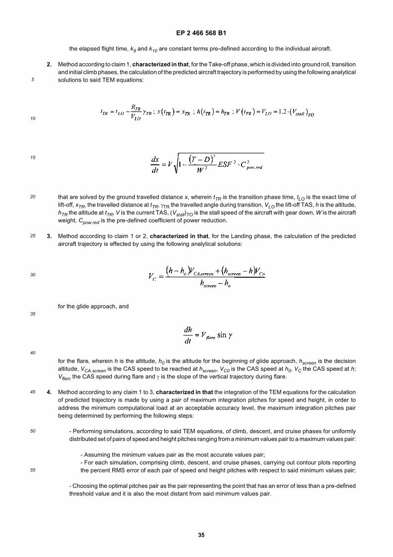
EP 2 466 568 B1

35

5

10

15

20

25

30

35

40

45

50

55

the elapsed flight time, k9 and k10 are constant terms pre-defined according to the individual aircraft.

2. Method according to claim 1, characterized in that, for the Take-off phase, which is divided into ground roll, transitionand initial climb phases, the calculation of the predicted aircraft trajectory is performed by using the following analyticalsolutions to said TEM equations:

that are solved by the ground travelled distance x, wherein tTR is the transition phase time, tLO is the exact time oflift-off, xTR, the travelled distance at tTR, γTR the travelled angle during transition, VLO the lift-off TAS, h is the altitude,hTR the altitude at tTR, V is the current TAS, (Vstall)TO is the stall speed of the aircraft with gear down, W is the aircraftweight, Cpow.red is the pre-defined coefficient of power reduction.

3. Method according to claim 1 or 2, characterized in that, for the Landing phase, the calculation of the predictedaircraft trajectory is effected by using the following analytical solutions:

for the glide approach, and

for the flare, wherein h is the altitude, h0 is the altitude for the beginning of glide approach, hscreen is the decisionaltitude, VCA.screen is the CAS speed to be reached at hscreen, VC0 is the CAS speed at h0, VC the CAS speed at h;Vflarc the CAS speed during flare and γ is the slope of the vertical trajectory during flare.

4. Method according to any claim 1 to 3, characterized in that the integration of the TEM equations for the calculationof predicted trajectory is made by using a pair of maximum integration pitches for speed and height, in order toaddress the minimum computational load at an acceptable accuracy level, the maximum integration pitches pairbeing determined by performing the following steps:

- Performing simulations, according to said TEM equations, of climb, descent, and cruise phases for uniformlydistributed set of pairs of speed and height pitches ranging from a minimum values pair to a maximum values pair:

- Assuming the minimum values pair as the most accurate values pair;- For each simulation, comprising climb, descent, and cruise phases, carrying out contour plots reportingthe percent RMS error of each pair of speed and height pitches with respect to said minimum values pair;

- Choosing the optimal pitches pair as the pair representing the point that has an error of less than a pre-definedthreshold value and it is also the most distant from said minimum values pair.

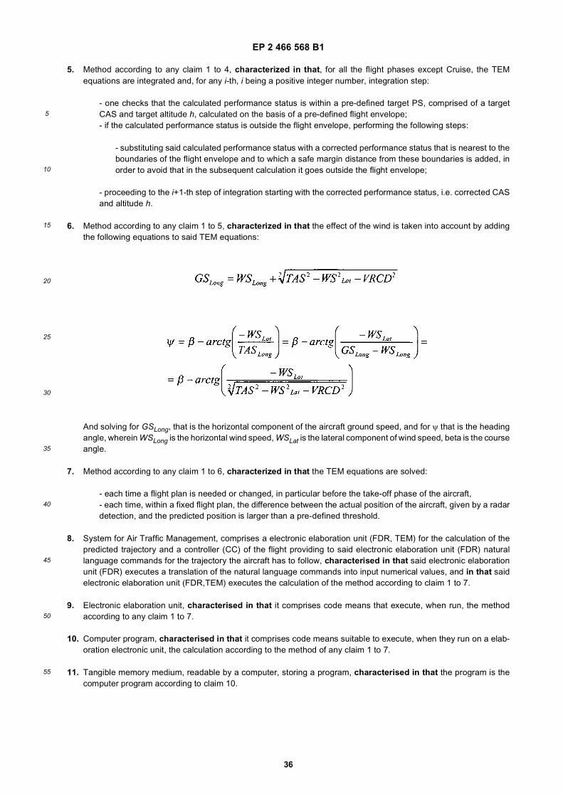
EP 2 466 568 B1

36

5

10

15

20

25

30

35

40

45

50

55

5. Method according to any claim 1 to 4, characterized in that, for all the flight phases except Cruise, the TEMequations are integrated and, for any i-th, i being a positive integer number, integration step:

- one checks that the calculated performance status is within a pre-defined target PS, comprised of a targetCAS and target altitude h, calculated on the basis of a pre-defined flight envelope;- if the calculated performance status is outside the flight envelope, performing the following steps:

- substituting said calculated performance status with a corrected performance status that is nearest to theboundaries of the flight envelope and to which a safe margin distance from these boundaries is added, inorder to avoid that in the subsequent calculation it goes outside the flight envelope;

- proceeding to the i+1-th step of integration starting with the corrected performance status, i.e. corrected CASand altitude h.

6. Method according to any claim 1 to 5, characterized in that the effect of the wind is taken into account by addingthe following equations to said TEM equations:

And solving for GSLong, that is the horizontal component of the aircraft ground speed, and for ψ that is the headingangle, wherein WSLong is the horizontal wind speed, WSLat is the lateral component of wind speed, beta is the courseangle.

7. Method according to any claim 1 to 6, characterized in that the TEM equations are solved:

- each time a flight plan is needed or changed, in particular before the take-off phase of the aircraft,- each time, within a fixed flight plan, the difference between the actual position of the aircraft, given by a radardetection, and the predicted position is larger than a pre-defined threshold.

8. System for Air Traffic Management, comprises a electronic elaboration unit (FDR, TEM) for the calculation of thepredicted trajectory and a controller (CC) of the flight providing to said electronic elaboration unit (FDR) naturallanguage commands for the trajectory the aircraft has to follow, characterised in that said electronic elaborationunit (FDR) executes a translation of the natural language commands into input numerical values, and in that saidelectronic elaboration unit (FDR,TEM) executes the calculation of the method according to claim 1 to 7.

9. Electronic elaboration unit, characterised in that it comprises code means that execute, when run, the methodaccording to any claim 1 to 7.

10. Computer program, characterised in that it comprises code means suitable to execute, when they run on a elab-oration electronic unit, the calculation according to the method of any claim 1 to 7.

11. Tangible memory medium, readable by a computer, storing a program, characterised in that the program is thecomputer program according to claim 10.

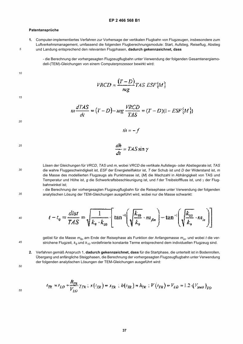
EP 2 466 568 B1

37

5

10

15

20

25

30

35

40

45

50

55

Patentansprüche

1. Computer-implementiertes Verfahren zur Vorhersage der vertikalen Flugbahn von Flugzeugen, insbesondere zumLuftverkehrsmanagement, umfassend die folgenden Flugberechnungsmodule: Start, Aufstieg, Reiseflug, Abstiegund Landung entsprechend den relevanten Flugphasen, dadurch gekennzeichnet, dass

- die Berechnung der vorhergesagten Flugzeugflugbahn unter Verwendung der folgenden Gesamtenergiemo-dell-(TEM)-Gleichungen von einem Computerprozessor bewirkt wird:

Lösen der Gleichungen für VRCD, TAS und m, wobei VRCD die vertikale Aufstiegs- oder Abstiegsrate ist; TASdie wahre Fluggeschwindigkeit ist, ESF der Energieteilfaktor ist, T der Schub ist und D der Widerstand ist, mdie Masse des modellierten Flugzeugs als Punktmasse ist, {M} die Machzahl in Abhängigkeit von TAS undTemperatur und Höhe ist, g die Schwerkraftsbeschleunigung ist, und f der Treibstofffluss ist, und γ der Flug-bahnwinkel ist;- die Berechnung der vorhergesagten Flugzeugflugbahn für die Reisephase unter Verwendung der folgendenanalytischen Lösung der TEM-Gleichungen ausgeführt wird, wobei nur die Masse schwankt:

gelöst für die Masse mfin am Ende der Reisephase als Funktion der Anfangsmasse min, und wobei t die ver-strichene Flugzeit, k9 und k10 vordefinierte konstante Terme entsprechend dem individuellen Flugzeug sind.

2. Verfahren gemäß Anspruch 1, dadurch gekennzeichnet, dass für die Startphase, die unterteilt ist in Bodenrollen,Übergang und anfängliche Steigphasen, die Berechnung der vorhergesagten Flugzeugflugbahn unter Verwendungder folgenden analytischen Lösungen der TEM-Gleichungen ausgeführt wird:

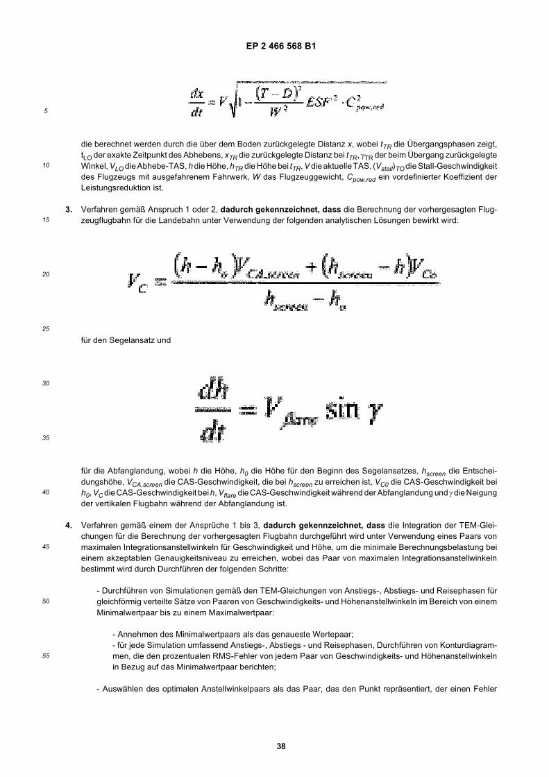
EP 2 466 568 B1

38

5

10

15

20

25

30

35

40

45

50

55

die berechnet werden durch die über dem Boden zurückgelegte Distanz x, wobei tTR die Übergangsphasen zeigt,tLO der exakte Zeitpunkt des Abhebens, xTR die zurückgelegte Distanz bei tTR, γTR der beim Übergang zurückgelegteWinkel, VLO die Abhebe-TAS, h die Höhe, hTR die Höhe bei tTR, V die aktuelle TAS, (Vstall)TO die Stall-Geschwindigkeitdes Flugzeugs mit ausgefahrenem Fahrwerk, W das Flugzeuggewicht, Cpow.red ein vordefinierter Koeffizient derLeistungsreduktion ist.

3. Verfahren gemäß Anspruch 1 oder 2, dadurch gekennzeichnet, dass die Berechnung der vorhergesagten Flug-zeugflugbahn für die Landebahn unter Verwendung der folgenden analytischen Lösungen bewirkt wird:

für den Segelansatz und

für die Abfanglandung, wobei h die Höhe, h0 die Höhe für den Beginn des Segelansatzes, hscreen die Entschei-dungshöhe, VCA.screen die CAS-Geschwindigkeit, die bei hscreen zu erreichen ist, VC0 die CAS-Geschwindigkeit beih0, VC die CAS-Geschwindigkeit bei h, Vflare die CAS-Geschwindigkeit während der Abfanglandung und γ die Neigungder vertikalen Flugbahn während der Abfanglandung ist.

4. Verfahren gemäß einem der Ansprüche 1 bis 3, dadurch gekennzeichnet, dass die Integration der TEM-Glei-chungen für die Berechnung der vorhergesagten Flugbahn durchgeführt wird unter Verwendung eines Paars vonmaximalen Integrationsanstellwinkeln für Geschwindigkeit und Höhe, um die minimale Berechnungsbelastung beieinem akzeptablen Genauigkeitsniveau zu erreichen, wobei das Paar von maximalen Integrationsanstellwinkelnbestimmt wird durch Durchführen der folgenden Schritte:

- Durchführen von Simulationen gemäß den TEM-Gleichungen von Anstiegs-, Abstiegs- und Reisephasen fürgleichförmig verteilte Sätze von Paaren von Geschwindigkeits- und Höhenanstellwinkeln im Bereich von einemMinimalwertpaar bis zu einem Maximalwertpaar:

- Annehmen des Minimalwertpaars als das genaueste Wertepaar;- für jede Simulation umfassend Anstiegs-, Abstiegs - und Reisephasen, Durchführen von Konturdiagram-men, die den prozentualen RMS-Fehler von jedem Paar von Geschwindigkeits- und Höhenanstellwinkelnin Bezug auf das Minimalwertpaar berichten;

- Auswählen des optimalen Anstellwinkelpaars als das Paar, das den Punkt repräsentiert, der einen Fehler

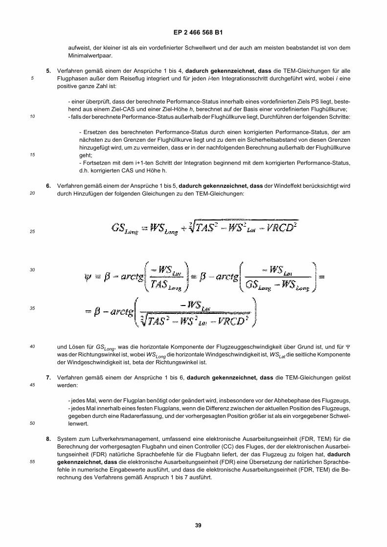
EP 2 466 568 B1

39

5

10

15

20

25

30

35

40

45

50

55

aufweist, der kleiner ist als ein vordefinierter Schwellwert und der auch am meisten beabstandet ist von demMinimalwertpaar.

5. Verfahren gemäß einem der Ansprüche 1 bis 4, dadurch gekennzeichnet, dass die TEM-Gleichungen für alleFlugphasen außer dem Reiseflug integriert und für jeden i-ten Integrationsschritt durchgeführt wird, wobei i einepositive ganze Zahl ist:

- einer überprüft, dass der berechnete Performance-Status innerhalb eines vordefinierten Ziels PS liegt, beste-hend aus einem Ziel-CAS und einer Ziel-Höhe h, berechnet auf der Basis einer vordefinierten Flughüllkurve;- falls der berechnete Performance-Status außerhalb der Flughüllkurve liegt, Durchführen der folgenden Schritte:

- Ersetzen des berechneten Performance-Status durch einen korrigierten Performance-Status, der amnächsten zu den Grenzen der Flughüllkurve liegt und zu dem ein Sicherheitsabstand von diesen Grenzenhinzugefügt wird, um zu vermeiden, dass er in der nachfolgenden Berechnung außerhalb der Flughüllkurvegeht;- Fortsetzen mit dem i+1-ten Schritt der Integration beginnend mit dem korrigierten Performance-Status,d.h. korrigierten CAS und Höhe h.

6. Verfahren gemäß einem der Ansprüche 1 bis 5, dadurch gekennzeichnet, dass der Windeffekt berücksichtigt wirddurch Hinzufügen der folgenden Gleichungen zu den TEM-Gleichungen:

und Lösen für GSLong, was die horizontale Komponente der Flugzeuggeschwindigkeit über Grund ist, und für Ψwas der Richtungswinkel ist, wobei WSLong die horizontale Windgeschwindigkeit ist, WSLat die seitliche Komponenteder Windgeschwindigkeit ist, beta der Richtungswinkel ist.

7. Verfahren gemäß einem der Ansprüche 1 bis 6, dadurch gekennzeichnet, dass die TEM-Gleichungen gelöstwerden:

- jedes Mal, wenn der Flugplan benötigt oder geändert wird, insbesondere vor der Abhebephase des Flugzeugs,- jedes Mal innerhalb eines festen Flugplans, wenn die Differenz zwischen der aktuellen Position des Flugzeugs,gegeben durch eine Radarerfassung, und der vorhergesagten Position größer ist als ein vorgegebener Schwel-lenwert.

8. System zum Luftverkehrsmanagement, umfassend eine elektronische Ausarbeitungseinheit (FDR, TEM) für dieBerechnung der vorhergesagten Flugbahn und einen Controller (CC) des Fluges, der der elektronischen Ausarbei-tungseinheit (FDR) natürliche Sprachbefehle für die Flugbahn liefert, der das Flugzeug zu folgen hat, dadurchgekennzeichnet, dass die elektronische Ausarbeitungseinheit (FDR) eine Übersetzung der natürlichen Sprachbe-fehle in numerische Eingabewerte ausführt, und dass die elektronische Ausarbeitungseinheit (FDR, TEM) die Be-rechnung des Verfahrens gemäß Anspruch 1 bis 7 ausführt.

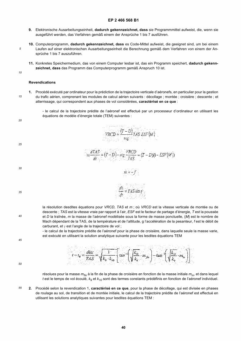
EP 2 466 568 B1

40

5

10

15

20

25

30

35

40

45

50

55

9. Elektronische Ausarbeitungseinheit, dadurch gekennzeichnet, dass sie Programmmittel aufweist, die, wenn sieausgeführt werden, das Verfahren gemäß einem der Ansprüche 1 bis 7 ausführen.

10. Computerprogramm, dadurch gekennzeichnet, dass es Code-Mittel aufweist, die geeignet sind, um bei einemLaufen auf einer elektronischen Ausarbeitungseinheit die Berechnung gemäß dem Verfahren von einem der An-sprüche 1 bis 7 auszuführen.

11. Konkretes Speichermedium, das von einem Computer lesbar ist, das ein Programm speichert, dadurch gekenn-zeichnet, dass das Programm das Computerprogramm gemäß Anspruch 10 ist.

Revendications

1. Procédé exécuté par ordinateur pour la prédiction de la trajectoire verticale d’aéronefs, en particulier pour la gestiondu trafic aérien, comprenant les modules de calcul aérien suivants : décollage ; montée ; croisière ; descente ; etatterrissage, qui correspondent aux phases de vol considérées, caractérisé en ce que :

- le calcul de la trajectoire prédite de l’aéronef est effectué par un processeur d’ordinateur en utilisant leséquations de modèle d’énergie totale (TEM) suivantes :

la résolution desdites équations pour VRCD, TAS et m ; où VRCD est la vitesse verticale de montée ou dedescente ; TAS est la vitesse vraie par rapport à l’air, ESF est le facteur de partage d’énergie, T est la pousséeet D la traînée, m la masse de l’aéronef modélisée sous la forme de masse ponctuelle, {M} est le nombre deMach dépendant de la TAS, de la température et de l’altitude, g l’accélération de la pesanteur, f est le débit decarburant, et γ est l’angle de la trajectoire de vol ;- le calcul de la trajectoire prédite de l’aéronef pour la phase de croisière, dans laquelle seule la masse varie,est exécuté en utilisant la solution analytique suivante pour les lesdites équations TEM

résolues pour la masse mfin à la fin de la phase de croisière en fonction de la masse initiale min, et dans lequelt est le temps de vol écoulé, k9 et k10 sont des termes constants prédéfinis en fonction de l’aéronef individuel.

2. Procédé selon la revendication 1, caractérisé en ce que, pour la phase de décollage, qui est divisée en phasesde roulage au sol, de transition et de montée initiale, le calcul de la trajectoire prédite de l’aéronef est effectué enutilisant les solutions analytiques suivantes pour lesdites équations TEM :

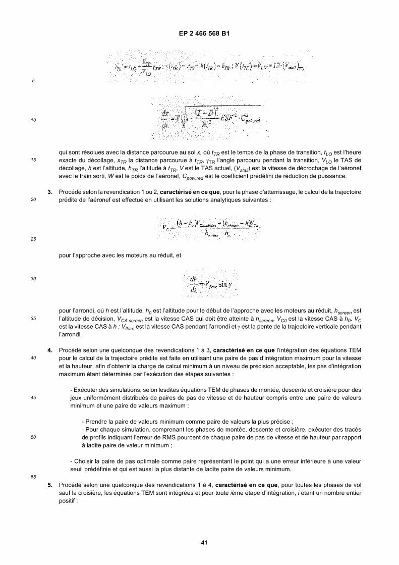
EP 2 466 568 B1

41

5

10

15

20

25

30

35

40

45

50

55

qui sont résolues avec la distance parcourue au sol x, où tTR est le temps de la phase de transition, tLO est l’heureexacte du décollage, xTR la distance parcourue à tTR, γTR l’angle parcouru pendant la transition, VLO le TAS dedécollage, h est l’altitude, hTR l’altitude à tTR, V est le TAS actuel, (Vstall) est la vitesse de décrochage de l’aéronefavec le train sorti, W est le poids de l’aéronef, Cpow.red est le coefficient prédéfini de réduction de puissance.

3. Procédé selon la revendication 1 ou 2, caractérisé en ce que, pour la phase d’atterrissage, le calcul de la trajectoireprédite de l’aéronef est effectué en utilisant les solutions analytiques suivantes :

pour l’approche avec les moteurs au réduit, et

pour l’arrondi, où h est l’altitude, h0 est l’altitude pour le début de l’approche avec les moteurs au réduit, hscreen estl’altitude de décision, VCA.screen est la vitesse CAS qui doit être atteinte à hscreen, VC0 est la vitesse CAS à h0, VCest la vitesse CAS à h ; Vflare est la vitesse CAS pendant l’arrondi et γ est la pente de la trajectoire verticale pendantl’arrondi.

4. Procédé selon une quelconque des revendications 1 à 3, caractérisé en ce que l’intégration des équations TEMpour le calcul de la trajectoire prédite est faite en utilisant une paire de pas d’intégration maximum pour la vitesseet la hauteur, afin d’obtenir la charge de calcul minimum à un niveau de précision acceptable, les pas d’intégrationmaximum étant déterminés par l’exécution des étapes suivantes :

- Exécuter des simulations, selon lesdites équations TEM de phases de montée, descente et croisière pour desjeux uniformément distribués de paires de pas de vitesse et de hauteur compris entre une paire de valeursminimum et une paire de valeurs maximum :

- Prendre la paire de valeurs minimum comme paire de valeurs la plus précise ;- Pour chaque simulation, comprenant les phases de montée, descente et croisière, exécuter des tracésde profils indiquant l’erreur de RMS pourcent de chaque paire de pas de vitesse et de hauteur par rapportà ladite paire de valeur minimum ;

- Choisir la paire de pas optimale comme paire représentant le point qui a une erreur inférieure à une valeurseuil prédéfinie et qui est aussi la plus distante de ladite paire de valeurs minimum.

5. Procédé selon une quelconque des revendications 1 è 4, caractérisé en ce que, pour toutes les phases de volsauf la croisière, les équations TEM sont intégrées et pour toute ième étape d’intégration, i étant un nombre entierpositif :

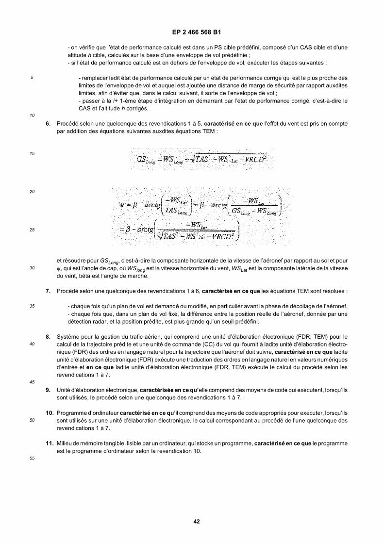
EP 2 466 568 B1

42

5

10

15

20

25

30

35

40

45

50

55

- on vérifie que l’état de performance calculé est dans un PS cible prédéfini, composé d’un CAS cible et d’unealtitude h cible, calculés sur la base d’une enveloppe de vol prédéfinie ;- si l’état de performance calculé est en dehors de l’enveloppe de vol, exécuter les étapes suivantes :

- remplacer ledit état de performance calculé par un état de performance corrigé qui est le plus proche deslimites de l’enveloppe de vol et auquel est ajoutée une distance de marge de sécurité par rapport auxditeslimites, afin d’éviter que, dans le calcul suivant, il sorte de l’enveloppe de vol ;- passer à la i+ 1-ème étape d’intégration en démarrant par l’état de performance corrigé, c’est-à-dire leCAS et l’altitude h corrigés.

6. Procédé selon une quelconque des revendications 1 à 5, caractérisé en ce que l’effet du vent est pris en comptepar addition des équations suivantes auxdites équations TEM :

et résoudre pour GSLong, c’est-à-dire la composante horizontale de la vitesse de l’aéronef par rapport au sol et pourψ, qui est l’angle de cap, où WSlong est la vitesse horizontale du vent, WSLat est la composante latérale de la vitessedu vent, bêta est l’angle de marche.

7. Procédé selon une quelconque des revendications 1 à 6, caractérisé en ce que les équations TEM sont résolues :

- chaque fois qu’un plan de vol est demandé ou modifié, en particulier avant la phase de décollage de l’aéronef,- chaque fois que, dans un plan de vol fixé, la différence entre la position réelle de l’aéronef, donnée par unedétection radar, et la position prédite, est plus grande qu’un seuil prédéfini.

8. Système pour la gestion du trafic aérien, qui comprend une unité d’élaboration électronique (FDR, TEM) pour lecalcul de la trajectoire prédite et une unité de commande (CC) du vol qui fournit à ladite unité d’élaboration électro-nique (FDR) des ordres en langage naturel pour la trajectoire que l’aéronef doit suivre, caractérisé en ce que laditeunité d’élaboration électronique (FDR) exécute une traduction des ordres en langage naturel en valeurs numériquesd’entrée et en ce que ladite unité d’élaboration électronique (FDR, TEM) exécute le calcul du procédé selon lesrevendications 1 à 7.

9. Unité d’élaboration électronique, caractérisée en ce qu’elle comprend des moyens de code qui exécutent, lorsqu’ilssont utilisés, le procédé selon une quelconque des revendications 1 à 7.

10. Programme d’ordinateur caractérisé en ce qu’il comprend des moyens de code appropriés pour exécuter, lorsqu’ilssont utilisés sur une unité d’élaboration électronique, le calcul correspondant au procédé de l’une quelconque desrevendications 1 à 7.

11. Milieu de mémoire tangible, lisible par un ordinateur, qui stocke un programme, caractérisé en ce que le programmeest le programme d’ordinateur selon la revendication 10.

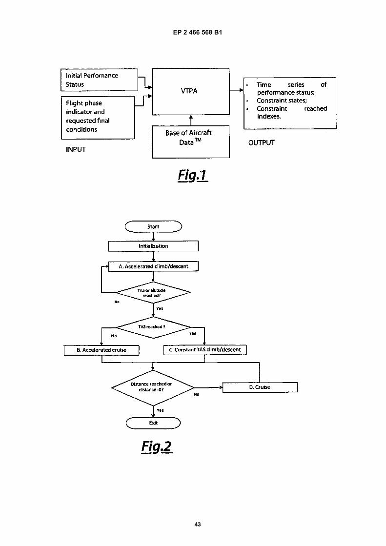
EP 2 466 568 B1

43

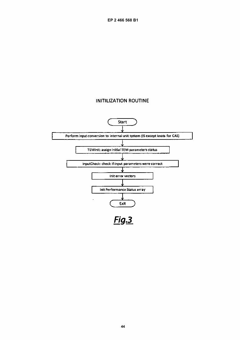
EP 2 466 568 B1

44

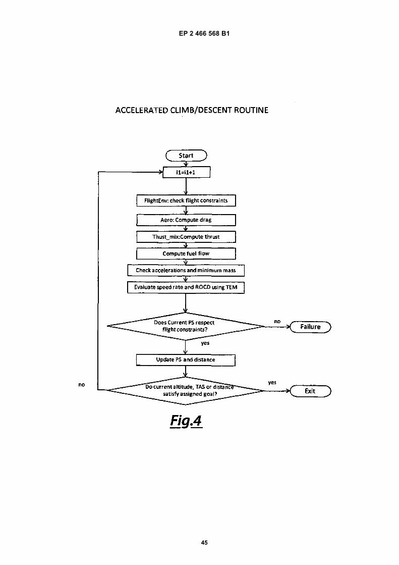
EP 2 466 568 B1

45

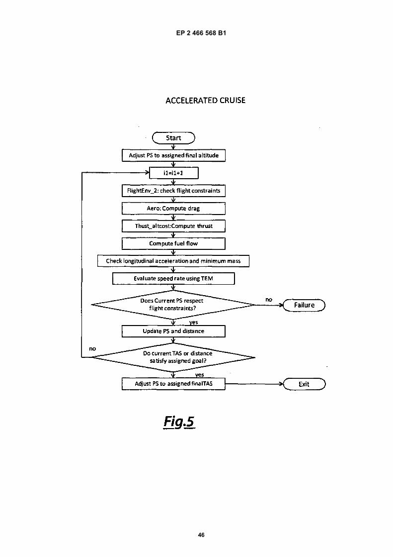
EP 2 466 568 B1

46

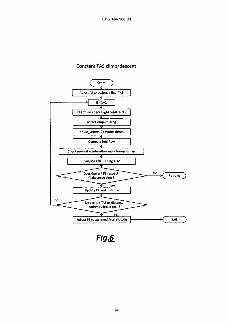
EP 2 466 568 B1

47

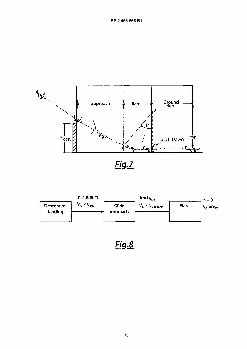
EP 2 466 568 B1

48

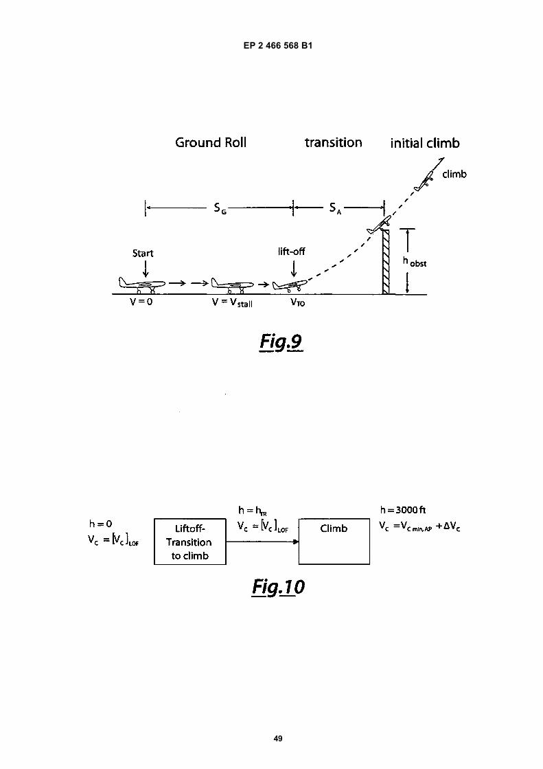
EP 2 466 568 B1

49

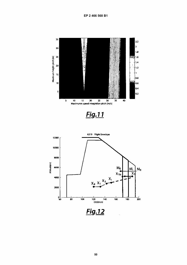
EP 2 466 568 B1

50

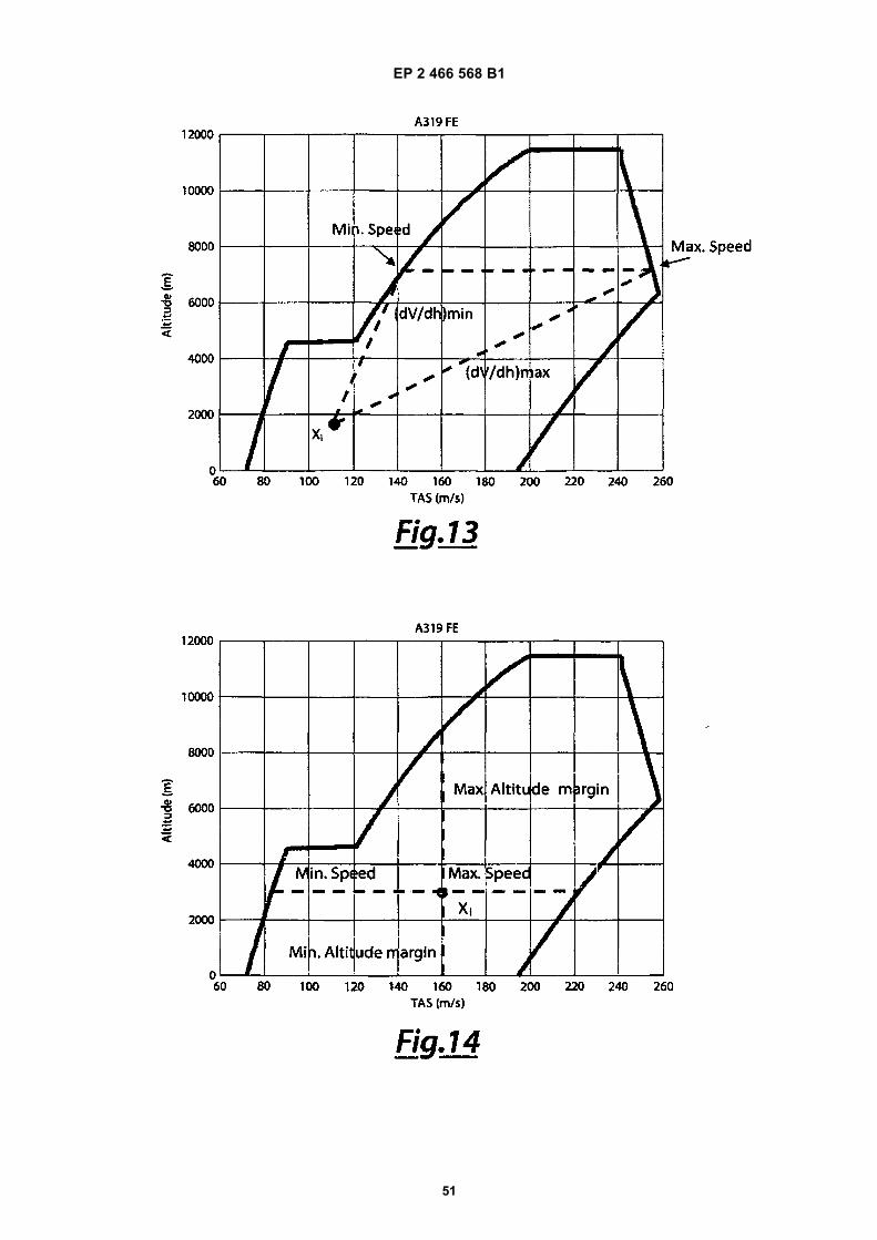
EP 2 466 568 B1

51

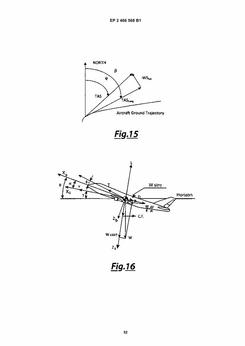
EP 2 466 568 B1

52

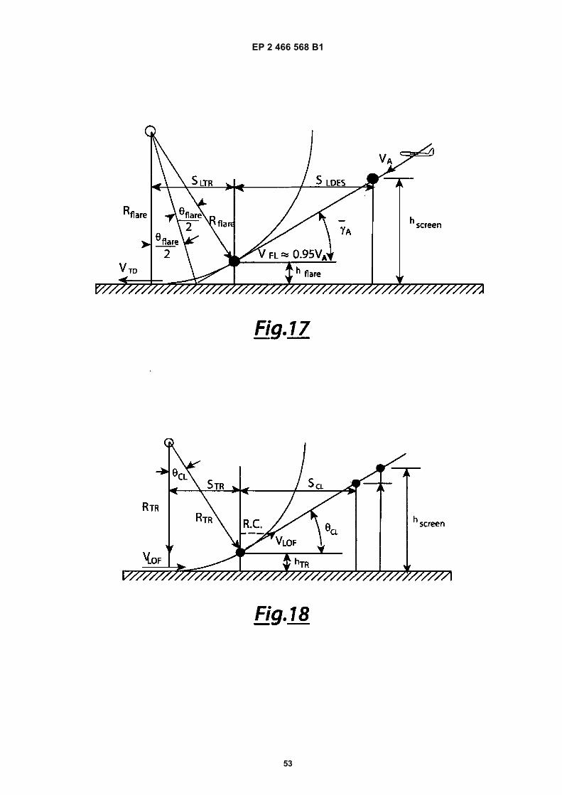
EP 2 466 568 B1

53

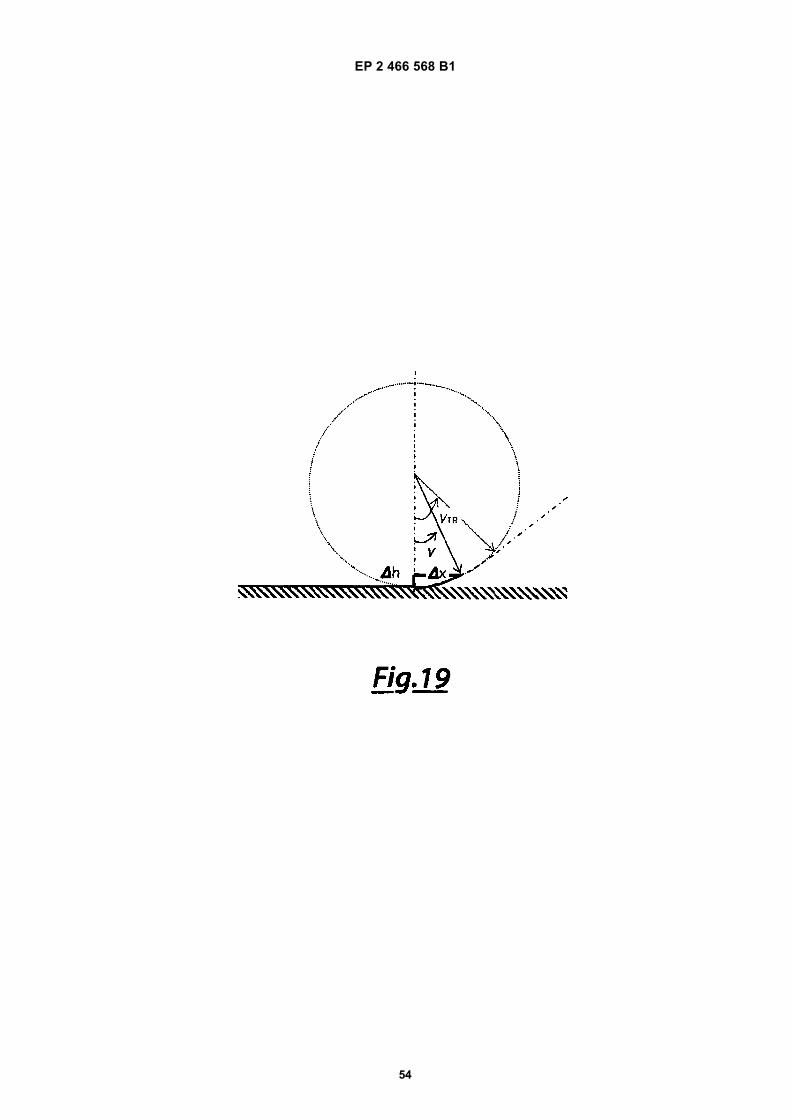
EP 2 466 568 B1

54

EP 2 466 568 B1

55

EP 2 466 568 B1

56

REFERENCES CITED IN THE DESCRIPTION

This list of references cited by the applicant is for the reader’s convenience only. It does not form part of the Europeanpatent document. Even though great care has been taken in compiling the references, errors or omissions cannot beexcluded and the EPO disclaims all liability in this regard.

Patent documents cited in the description

• WO 2007072028 A [0012]

Non-patent literature cited in the description

• SLATTERY, R. ; ZHAO, Y. Trajectory Synthesis forAir Traffic Automation. AIAA Journal of Guidance,Control, and Dynamics, March 1997, vol. 20 (2),232-238 [0010]

• SWENSON, H. N. ; HOANG, T. ; ENGELLAND, S. ;VINCENT, D. ; SANDERS, T. ; SANFORD, B. ;HEERE, K. Design and Operational Evaluation of theTraffic Management Advisor at the Fort Worth AirRoute Traffic Control Center. 1st USA/Europe AirTraffic Management Research and DevelopmentSeminar, Saclay, France, June 1997 [0010]

• A Stochastic Hybrid model for Air Traffic Control Sim-ulation. GLOVER, W. ; LYGEROS, J. HybridSystems : Computation and Control, ser. LNCS.Springer Verlag, 2004, 372-386 [0010]

• MARCO PORRETTA ; MARIE-DOMINIQUEDUPUY ; WOLFGANG SCHUSTER ; ARNABMAJUMDAR ; WASHINGTON OCHIENG. Perform-ance Evaluation of a Novel 4D Trajectory PredictionModel for Civil Aircraft. The Journal of Navigation,2008, vol. 61, 393-420 [0010]

• User Manual for the Base of Aircraft Data (BADA) -Revision 3.6. NUIC, A. EUROCONTROL, EEC NoteNo. 10/04. July 2004 [0209]

• PAMADI, B.N. Performance, Stability, Dynamics,and Control of Airplanes. American Institute of Aero-nautics and Astronautics, 2004 [0209]

• ROSKAM, J ; CHAN-TAU, E. L. Airplane Aerody-namics and Performance, 1997 [0209]

• SESAR Consortium, Work Programme for2008-2013, Doc. SESAR Consortium No.DLM-0710-002-01-00, April 2008 [0209]

• Joint Planning and Development Office, Concept ofOperations for the Next Generation Air TransporationSystem, v.2.0, June 2007 [0209]

• CISTONE, J. Next Century Aerospace Traffic Man-agement: The Sky is No Longer the Limit. AIAA Jour-nal of Aircraft, 2004, vol. 41 (1), 36-42 [0209]

• WU, S.F. ; GUO, S.F. Optimum Flight TrajectoryGuidance Based on Total Energy Control of Aircraft.AIAA Journal of Guidance, Control, and Dynamics,vol. 17 (2), 291-296 [0209]

• SLATTERY, R. ; ZHAO, Y. Trajectory Synthesis forAir Traffic Automation. AIAA Journal of Guidance,Control, and Dynamics, 1997, vol. 20 (2), 232-238[0209]

• DUPUY, M.D. ; PORRETTA, M. Preliminary resultsfor a robust trajectory prediction method using ad-vanced flight data. IEEE/AIAA 26th Digital AvionicsSystems Conference, IEEE, Dallas, TX, 2007,1.C.5-11.C.5-9 [0209]

• GALLO, E. ; LOPEZ-LEONES, J. ; VILAPLANA,M.A.E. ; NAVARRO, F.A. ; NUIC, A. Trajectory com-putation Infrastructure based on BADA Aircraft Per-formance Model. IEEE/AIAA 26th Digital AvionicsSystems Conference, IEEE, Dallas, TX, 2007,1.C.4-11.C.4-13 [0209]

• MONDOLONI, S. Development Of Key PerformanceIndicators for Trajectory Prediction Accuracy.IEEE/AIAA 26th Digital Avionics Systems Confer-ence, IEEE, Indianapolis, IN, 2006, 1-11 [0209]

• NUIC, A. ; POINSOT, C. ; LAGARU, M-G. ; GALLO,E. ; NAVARRO, F.A. ; QUEREJETA, C. AdvancedAircraft Performance Modeling for ATM: Enhance-ments to the Bada Model. IEEE/AIAA 25th Digital Av-ionics Systems Conference, IEEE, Washington, DC,2005, 1-12 [0209]

• MINKA, T. The Lightspeed Matlab Toolbox. MicrosoftInc, 2006 [0209]