Multi-functional Lagrangian flow structures in three-dimensional ac electro-osmotic micro-

flows

This article has been downloaded from IOPscience. Please scroll down to see the full text article.

2011 Fluid Dyn. Res. 43 035503

(http://iopscience.iop.org/1873-7005/43/3/035503)

Download details:

IP Address: 187.195.211.230

The article was downloaded on 26/01/2013 at 03:17

Please note that terms and conditions apply.

View the table of contents for this issue, or go to the journal homepage for more

Home Search Collections Journals About Contact us My IOPscience

IOP PUBLISHING FLUID DYNAMICS RESEARCH

Fluid Dyn. Res. 43 (2011) 035503 (24pp) doi:10.1088/0169-5983/43/3/035503

Multi-functional Lagrangian flow structures inthree-dimensional ac electro-osmotic micro-flows

M F M Speetjens, H N L de Wispelaere and A A van Steenhoven

Energy Technology Laboratory, Department of Mechanical Engineering, Eindhoven Universityof Technology, PO Box 513, 5600 MB, Eindhoven, The Netherlands

E-mail: m.f.m.speetjens@tue.nl

Received 9 December 2010, in final form 1 March 2011Published 18 April 2011Online at stacks.iop.org/FDR/43/035503

Communicated by Mitsu Funakoshi

AbstractFlow forcing by ac electro-osmosis (ACEO) is a promising technique forthe actuation and manipulation of micro-flows. Utilization to date mainlyconcerns pumping and mixing. However, emerging micro-fluidic applicationsdemand further functionalities. The present study explores the first ways tosystematically realize this in three-dimensional (3D) micro-flows using ACEO.This exploits the fact that continuity ‘organizes’ Lagrangian fluid trajectoriesinto coherent structures that geometrically determine the transport properties.Lagrangian flow structures typically comprise families of concentric tubularstructures, acting both as transport barriers and as transport conduits,embedded in chaotic regions. Numerical simulations of representative casestudies demonstrate that ACEO, possibly in combination with other forcingmechanisms, has the potential to tailor these features into multi-functionalLagrangian flow structures that can fulfill various transport purposes. This maygreatly enhance the functionality and versatility of labs-on-a-chip.

(Some figures in this article are in colour only in the electronic version)

1. Introduction

Flow forcing by ac electro-osmosis (ACEO) is a promising technique for the actuationand manipulation of micro-flows (Ramos et al 1999, Green et al 2002, Stone et al 2004,Squires 2009, Aboelkassem 2010, Chen et al 2010, Kim et al 2010). Primary micro-fluidicapplications to date include pumping (Ramos et al 2003, 2005, Bazant and Ben 2006,Urbanski et al 2006, 2007, Kuo and Liu 2008) and mixing (Chang and Yang 2004, Nguyenand Wu 2005, Meisel and Ehrhard 2006, Pacheco et al 2006, 2008, Chen et al 2009,Meijer et al 2009). However, emerging (lab-on-a-chip) technologies, e.g. molecular analysisand biotechnology, demand further functionalities including the establishment of specific

© 2011 The Japan Society of Fluid Mechanics and IOP Publishing Ltd Printed in the UK0169-5983/11/035503+24$33.00 1

Fluid Dyn. Res. 43 (2011) 035503 M F M Speetjens et al

temperature or concentration fields and targeted delivery of heat and mass in designatedflow regions (Beebe et al 2002, Hansen and Quake 2003, Tourovskaia et al 2005, Pearceand Williams 2007, Mills et al 2008, Meagher et al 2008, Weigl et al 2008). ACEO seemsparticularly suited for the realization of such multi-functional micro-flows, in that cleverdesign of the electrode layout and geometry in combination with variable spatiotemporal acsignals offers great control over the internal flow (Ramos et al 2003, 2005 Squires 2009,Chen et al 2010, Kim et al 2010). This motivates this study, which explores the first ways tosystematically achieve generic transport functionalities in three-dimensional (3D) micro-flowsusing ACEO.

Fundamental to micro-fluidic transport is that it happens under laminar flow conditions(Ottino and Wiggins 2004, Stone et al 2004, Tabeling 2009). This implies a strong disparitybetween a flow and its transport properties in that simple and regular flow patterns maycoexist with complicated transport properties. (A well-known example is chaotic fluidadvection in simple flows (Aref 2002).) This advances a Lagrangian (i.e. fluid-parcel-based)representation as the most natural description for laminar transport Ottino 1989, Wiggins andOttino 2004, Funakoshi 2008. Continuity ‘organizes’ the Lagrangian fluid trajectories intospecific coherent structures that geometrically determine the transport properties (Cartwrightet al 1996, Speetjens et al 2004). This notion admits visualization and analysis of laminartransport by identification of such ‘elementary building blocks’. Moreover, this fundamentalgeometric organization, in principle, enables the systematic creation and destruction ofcoherent structures for specific transport purposes.

Studies of micro-fluidic Lagrangian transport primarily concern the transverse mixingof axial fluid streams in 3D steady flow within infinite micro-channels (Chang and Yang2004, Nguyen and Wu 2005, Meisel and Ehrhard 2006, Pacheco et al 2006, 2008, Chenet al 2009, Meijer et al 2009). This configuration is directly modelled on—and dynamicallyentirely analogous to—macroscopic inline viscous mixers (Bertsch et al 2001, Kim et al2004, Mizuno and Funakoshi 2004). Flow is usually presumed periodic and uni-directional inthe axial direction, admitting reduction of Lagrangian transport to an axial map between theinlet and the outlet of periodic channel compartments. This map is for incompressible flowsessentially equivalent to the well-known Hamiltonian maps, causing the characteristic 3DLagrangian flow structures consisting of longitudinal stream tubes embedded in chaotic seas(Ottino 1989, Kim et al 2004, Ottino and Wiggins 2004, Pacheco et al 2006, Speetjens et al2006a, Funakoshi 2008, Pacheco et al 2008). These tubes act as transport barriers and theirdestruction into chaotic regions by triggering Hamiltonian breakdown mechanisms throughthe flow forcing is the principal aim in mixing flows.

The present study demonstrates that ACEO has the potential for manipulation of transportproperties beyond that of destruction of (tubular) transport barriers for mixing purposes—even in a standard periodic micro-channel. This exploits the fact that incompressible 3Dsteady flows devoid of a global uni-directional component in essence consist of multipleflow regions that each separately exhibit the Hamiltonian dynamics described above forinline (micro-)mixers. The generic Lagrangian flow structure, in consequence, encompassesmultiple families of tubular transport barriers embedded within chaotic regions. The particulararrangement and states of disintegration of said tubes depends essentially on the flowforcing, however. This affords promising practical opportunities in that ACEO, possiblyin combination with another forcing (e.g. pressure gradients or dc electro-osmosis), thusfacilitates systematic manipulation of the Lagrangian flow structure for a wide range oftransport purposes. This paves the way for a much greater functionality than pumping andmixing alone. Moreover, it offers great flexibility by (in principle) enabling the realization ofmultiple Lagrangian flow structures within one and the same micro-channel.

2

Fluid Dyn. Res. 43 (2011) 035503 M F M Speetjens et al

0

(a) (b)

Figure 1. 3D ACEO configuration: (a) periodic flow domain including electrodes and (b) typicalaxial slip velocity on the bottom wall.

The present study investigates the generic 3D Lagrangian flow structure inside periodicmicro-channels due to ACEO forcing and the basic mechanisms for its manipulation.Moreover, it widens the exploration of said structure to potential applications other thanmixing. To this end, true 3D steady flow including fluid inertia and without a global uni-directional component is considered. This approach sets the current investigation apartfrom other Lagrangian analyses to date; the latter in general concern 2D/2.5D/non-inertialapproximations with uni-directional axial flow and exclusively concentrate on mixing(Khakhar et al 1987, Chang and Yang 2004, Metcalfe et al 2006, Meisel and Ehrhard2006, Pacheco et al 2006, 2008). The numerical scheme combines commercial CFD toolsfor the flow field with dedicated algorithms for the electrokinetic problem and Lagrangiantrajectories. This strategy provides maximal flexibility at sufficient accuracy for the simulationof Lagrangian flow structures (Hobbs and Muzzio 1998).

This paper is organized as follows. Section 2 introduces the physical problem and theconfiguration investigated here. The theoretical framework of Lagrangian flow structures isoutlined in section 3, and section 4 elaborates on the numerical strategy. The basic Lagrangiancomposition of ACEO flows is examined in section 5 and its emergence in more complexmicro-fluidic systems is demonstrated in section 6. Performance of the numerical scheme isevaluated in section 7 and the conclusions drawn are presented in section 8.

2. Problem definition

2.1. Introduction

The flow domain consists of a 3D rectangular channel D : [x, y, z] = [0, 2L] × [0, H ] ×

[0, L] with the periodic inlet (x = 0) and outlet (x = 2L). Two electrodes of width We andspacing Ws = L − We are placed parallel to the z-axis at the bottom wall within intervalsWs/26 x 6 L − Ws/2 and L + Ws/26 x 6 2L − Ws/2 (figure 1(a)). ACEO triggered bythese electrodes induces a slip velocity on the bottom wall (figure 1(b)) that sets up aninternal flow comprising electrodewise pairs of counter-rotating vortices (figure 1(a)) andsmall vortices near the electrode edges (not shown). Rescaling by L yields the associated non-dimensional domain D : [x, y, z] = [0, 2] × [0, D] × [0, 1], with D = H/L being the verticalaspect ratio andWe = We/L ,Ws = Ws/L the corresponding electrode dimensions.

2.2. Electrokinetic problem

ACEO is described by the linear model according to Ramos et al (2005). This hinges on twoassumptions: (i) the voltage V (t) = V0sin(ωt), with ω being the ac angular frequency, applied

3

Fluid Dyn. Res. 43 (2011) 035503 M F M Speetjens et al

to the electrodes is small enough to prevent electrolysis; (ii) the electric double layer (EDL) isin a quasi-equilibrium (i.e. ω � τ−1

EDL , with τEDL = ε/σ being the relaxation time of the cyclicEDL charging, ε the permittivity and σ the conductivity). This implies that the EDL acts asan ideal capacitor (capacitance CDL) and means that the electrical potential 8 in the bulk fluidis described by the potential problem

∇28 = 0,

σ

CDL

∂8

∂y

∣∣∣∣e

=∂

∂t(8 − V )

∣∣∣∣e

,∂8

∂y

∣∣∣∣g

= 0, 8|y=D = 0, (1)

where ‘e’ and ‘g’ denote electrode and glass segments on the bottom wall, respectively,and 8(x)|x=0 = 8(x)|x=2 due to the periodic inlet–outlet. Moreover, the arrangement ofthe electrodes parallel to the z-axis means transverse variations are absent, reducing theelectrokinetic system to a 2D problem for 8 = 8(x, y).1

The ion flux induced by the electric field gives rise to a slip velocity directly above theelectrodes that effectively acts as a ‘driving wall’ for the fluid. However, the ac frequency ω issuch that the fluid cannot follow the instantaneous changes in ion propagation direction and,in consequence, ‘feels’ only the time-averaged slip velocity

〈uslip〉(x) = −ε3

4µ

∂

∂x

(|8 − V0|

2), (2)

with 3 = CDL/CD being the ratio of capacitances of the EDL and diffusive layer. Thenegligible potential drop at the glass/electrolyte interfaces results in a zero slip velocity(Ramos et al 2005).

2.3. Fluid dynamics

The 3D flow field u(x) is governed by the steady incompressible Navier–Stokes equations

∇ · u = 0, u · ∇u = −1

ρ∇ p + ν∇

2u, (3)

with p = p − ρgy being the dynamic pressure, ρ the fluid density and ν its kinematicviscosity. Here, spatial periodicity, similar as before, means u(x)|x=0 = u(x)|x=2. Theflow is subject to the no-slip condition u = 0 on the top wall (y = D), sidewalls (z =

0, 1) and between the electrodes at the bottom wall. The time-averaged slip velocity (2)is imposed on the electrodes: u|electrode = [〈uslip〉(x), 0, 0]. The electrokinetic phenomenamanifest themselves only through this slip velocity; internal electric body forces are absent inthe present approximation. Hence, only a one-way coupling between electrokinetics and fluiddynamics exists.

2.4. Non-dimensional formulation

The corresponding non-dimensional form follows from rescaling the relevant quantities viax ′

= x/L , t ′= t/τRC, 8′

= 8/V0, V ′= V/V0, u′

= u/U and p′= p/P , with L as before,

τRC = CDL L/σ , U = max(〈uslip〉) and P = ρνU/L . (The pressure scale stems from assumingthat a balance between pressure and viscous forces dominates the momentum equation.)

1 The homogeneous Dirichlet condition for the potential 8 at the top wall presumes a sufficient distance D tothe bottom wall for the electric field to remain restricted to the lower part of the domain. Alternative conditions for‘close’ top and bottom walls are an electrically insulated top wall, translating into a homogeneous Neumann condition∂8/∂y|y=D = 0.

4

Fluid Dyn. Res. 43 (2011) 035503 M F M Speetjens et al

Substitution into (1) and (3) gives

∇′28′

= 0,∂8′

∂y′

∣∣∣∣e

=∂

∂t ′

(8′

− V ′) ∣∣∣∣

e

,∂8′

∂y′

∣∣∣∣g

= 0, 8′|y=D = 0 (4)

and

∇′· u′

= 0, Re u′· ∇

′u′= −∇

′ p′ + ∇′2u′, (5)

respectively, with V ′(t) = sin(wt) and 〈u′

slip〉(x) = −5∂/∂x(|8′− 1|

2) being the corre-sponding ac signal and slip velocity. Here 5 = εV 2

0 3/4µU L is a scaling factor ensuringmax(〈u′

slip〉) = 1. Note that prime signs are omitted hereafter for brevity.The above exposes, in addition to (D,We,Ws) defined in section 2.1, the Reynolds

number Re = U L/ν and the dimensionless ac frequency ω = ωτRC as relevant non-dimensional parameters. Parameters are fixed at D = 0.5, We = 0.6, Ws = 0.4 and ω = 1,leaving Re as the single system parameter in the analysis below. Further degrees of freedominclude the electrode configuration and combination with other forcing mechanisms. Fluidmotion is considered under inertial conditions (Re > 0) as well as in the non-inertial limit(Re = 0). The momentum equation in (5) simplifies to the well-known Stokes equationsubject to the rescaled slip velocity defined before in the latter case. Hence, Re = 0 doesnot imply vanishing slip velocity.

3. Lagrangian transport analysis by Hamiltonian mechanics

Laminar transport is an essentially Lagrangian phenomenon (qualitatively) determined by thetopological properties of the fluid trajectories. The continuity constraint ∇ · u = 0 ‘organizes’these trajectories into coherent structures that collectively define the flow topology andgeometrically determine fluid advection (Ottino 1989, Aref 2002, Speetjens et al 2004,Wiggins and Ottino 2004).

The motion of fluid parcels is governed by the 3D autonomous kinematic equation

dxdt

= u(x) ⇒ x(t) =Φt (x0), (6)

describing the Lagrangian fluid trajectories originating from initial positions x0. Thesetrajectories coincide with streamlines of u in the present study due to steady flow. Continuityenables (local) recasting of (6) into the 2D Hamiltonian system

dη

dξ=

∂H∂ζ

,dζ

dξ= −

∂H∂η

, ⇒ x′(ξ) =Φ′

ξ (x′

0), (7)

with x′= (η, ζ ), everywhere outside stagnation points u = 0 via the (local) coordinate

transformation F : (x, y, z) → (η, ζ, ξ) (Bajer 1994, Speetjens et al 2006a). The functionH=H(η, ζ, ξ) represents the Hamiltonian; variables x′ and ξ define the correspondingspatial and temporal coordinates, respectively. Thus the present ACEO flows, save in theproximity of (possible) stagnation points, in essence exhibit Hamiltonian dynamics. This hasfundamental ramifications for the composition and behavior of the flow topology.

The key coherent structures of Hamiltonian flow topologies are tori. In system (7), theyappear as families of concentric closed orbits defining island-like structures (‘elliptic islands’)in the 2D (η, ζ )-domain and tubes in the 3D space–time domain (η, ζ, ξ) (Ottino 1989). Inthe 3D spatially periodic steady flow, they may emerge in two kinds: firstly, as stream tubesconnecting the periodic inlet–outlet. The cross-sections (y, z) and the axial coordinate x thentransform into (η, ζ ) and ξ , respectively, meaning that the axial flow ux acts as a fictitious

5

Fluid Dyn. Res. 43 (2011) 035503 M F M Speetjens et al

ζ

ηξ

ζ

ηξ

(a) (b)

Figure 2. Two kinds of physical appearance of tori in 3D steady flows: (a) stream tubes connectingthe periodic inlet–outlet and (b) closed stream tubes within the domain interior.

evolution in time (Speetjens et al 2006a). Secondly, as closed stream tubes withinD (Speetjenset al 2006b). Here the cross-section and the secondary axis of the tori correspond to (η, ζ ) andξ , respectively. Furthermore, the closedness of the tori implies a time-periodic-associated 2DHamiltonian system, i.e. H(η, ζ, ξ) =H(η, ζ, ξ + τ), with τ being some (typically family-dependent) period time τ . Streamlines are limit cases in that they correspond to tori withcross-sections collapsing on a single point. Both kinds of physical appearance of tori areillustrated in figure 2; heavy curves outline the 2D (η, ζ )-domain.

The periodic evolution within families of tori admits reduction of the continuous flow inthe Hamiltonian formulation (7) to a map

x′

k+1 =Φ′

τ (x′

k), x′

k = x′(kτ), (8)

with the sequence of positions X ′(x′

0) = [x′

0, x′

1, x′

2, . . .] within the 2D (η, ζ )-domain (heavycurves in figure 2). This constitutes the so-called Poincaré section of the trajectory originatingfrom the position x′

0 (Ott 2002). Time levels ξ = kτ (k = 0, 1, . . .) correspond to fixed spatialcross-sections of the 3D stream tubes.

The 3D transport properties are inextricably linked to Hamiltonian response scenarios ofthe flow topology to perturbation introduced by e.g. the flow forcing. For ‘weak’ perturbationsthree basic responses may occur:

(a) Perturbation of closed streamlines causes coalescence into families of tori (Cartwrightet al 1996).

(b) Perturbation of rational tori causes break-up into multiple families of tori embedded inchaotic bands according to the Poincaré–Birkhof theorem (Ottino 1989, Ott 2002).

(c) Perturbation of irrational tori causes survival in a slightly deformed manner accordingto the Kolmogorov–Arnold–Moser theorem (Ottino 1989, Ott 2002).

Tracers on a rational torus resume initial positions after a finite number of revolutionsand thus describe closed streamlines wound around its surface. Tracers on an irrationaltorus describe non-closed streamlines that densely fill its surface. The response to ‘strong’perturbations is essentially nonlinear and case-specific and may yet not must result inprogressive disintegration of surviving tori into a state of total chaos (Ott 2002, Speetjenset al 2006a). Thus flow topologies basically consist of (remnants of) tori situated in a chaoticenvironment and subject to the above response scenarios. This allows a systematic strategyfor Lagrangian transport studies.

6

Fluid Dyn. Res. 43 (2011) 035503 M F M Speetjens et al

Figure 3. Reduction of the flow domain due to spatial symmetries. Solid and dashed lines outlinethe reduced and the original domain, respectively.

4. Numerical methods

4.1. Computational domain

Symmetry considerations imply that the electrokinetic and flow fields exhibit reflectionalsymmetry about the midplane z = 0.5 and x-wise translational symmetry x → x + 1. Thisadmits reduction of the flow domain D to the elementary subdomain D∗ : [x, y, z] = [0, 1] ×

[0, D] × [0, 0.5] (figure 3). This signifies a decrease in size—and, inherently, in computationaleffort—by a factor of four. Important to note is that the translational symmetry implies thatthe inlet x = 0 and the cross-section x = 1, similar to the periodic inlet–outlet, also form aperiodic pair.

4.2. Electrokinetic problem

The one-way coupling between electrokinetics and fluid dynamics (section 2.3) admitsseparate resolution of the electrokinetic model (4) within the reduced domain D∗. Numericaltreatment embarks on Fourier expansion of ac signal and potential via

V (t) =

∑m

Vm exp(iωm t), 8(x, t) =

∑m

8m(x) exp(iωm t), (9)

which upon substitution into (4) yields

∇28m = 0,

∂8m

∂y

∣∣∣∣e

= iωm

(8m − Vm

) ∣∣∣∣e

,∂8m

∂y′

∣∣∣∣g

= 0, 8m |y=D = 0, (10)

as the governing model for each Fourier mode m. Spatial discretization of (10) employs astandard 2D spectral method based on x-wise and y-wise expansion of potential 8 by theFourier and Chebyshev polynomials, respectively, and incorporates boundary conditions bythe Lanczos tau method (Canuto et al 1987). Bottom-wall conditions in (10) are lumped via

∂8m

∂y

∣∣∣∣y=0

= iωm

(8m − Vm

)[F(x) + F(x − 1)], (11)

with F = H(x −Ws/2) − H(x − 1 +Ws/2) and H(x) = [tanh(x/W ) + 1]/2 the smoothedHeaviside function, so as to attain a smooth transition from electrodes to intermediateglass sections within a narrow region of width W (here W = 1/8π ≈ 0.04). This ensuresexponential convergence and thereby very accurate resolution (Canuto et al 1987). Thealgorithm is implemented in the high-level programming language MATLAB.

7

Fluid Dyn. Res. 43 (2011) 035503 M F M Speetjens et al

4.3. Flow field

The flow field follows from numerical simulation of (5) in D∗ by way of the finite-volume-method (FVM) package FLUENT (standard solver with second-order upwind scheme forthe inertial term). Periodic boundary conditions are imposed on x = 0 and x = 1 (outlet ofreduced domain D∗); conditions on stationary wall (segments) and symmetry plane z = 0.5are implemented via standard no-slip and symmetry conditions. The slip velocity 〈u′

slip〉 iscomputed from the simulated electric potential and incorporated in FLUENT through user-defined functions. Smoothed electrokinetic conditions via (11) avoid velocity singularities atthe electrode edges. This enables accurate resolution near these edges with sufficiently smallyet finite mesh sizes 1x � W .

The basic FVM mesh for D∗ consists of hexahedral elements defined by anequidistant grid of nD = nx × ny × nz = 250 × 80 × 50 = 106 nodes and (1x, 1y, 1z) =

(0.004, 0.0063, 0.01) as corresponding spacings. This mesh meets the above resolutioncriterion 1x � W . Additional local grid refinement nonetheless proves to be crucial. Highlyaccurate resolution of continuity namely is critical for the simulation of Lagrangian tracerpaths (Speetjens and Clercx 2005). To this end, progressive refinement toward the bottomwall using the Chebyshev–Gauss–Lobatto distribution y j = D(1 − cos(π j/2Ny)), with 06j 6 Ny and Ny the number of nodes in the y-direction, within the layer 06 y 61D has beencarried out (Canuto et al 1987). Tests expose 1D ≈ D/10 and Ny ≈ 40 as the optimal heightand nodal density, respectively, augmenting the mesh to nD ≈ 1.4 × 106 nodes. Important tonote is that adaptive grid refinement by FLUENT on the basis of velocity gradients results instrong refinement near the electrode edges, yet with only marginal improvement.

4.4. Lagrangian tracer paths

Lagrangian tracer paths are determined through simulation of the kinematic equation (6) by adedicated tracking algorithm implemented in MATLAB. Integration of (6) occurs with a third-order Taylor–Galerkin scheme

xm+1/3 = xm +1t

3u(xm),

xm+1/2 = xm +1t

2u(xm+1/3), (12)

xm+1 = xm + 1tu(xm+1/2),

with adaptive time steps set via 1t = l/|u(xm)|, where l < min(1x, 1x, 1z) is a presetmaximum displacement and bounding by 1tmin 61t 61tmax. (Here 1tmin = 10−4 and1tmax = 0.05.) Interpolation of the steady-state flow field u from the FLUENT grid ontoarbitrary positions xm employs the built-in MATLAB routine griddata3 (linear interpolationbased on the Delaunay triangulation) for the local data set comprising the 33

= 27 (interior)or 23

= 8 (wall region) nearest nodes.

5. Flow topologies in basic ACEO flows

5.1. Introduction

Figure 4 gives the planar velocity field (ux , u y) in the 2D cross section z = 0.25 (panel (a),top) and the normal vorticity ωz = ∂u y/∂x − ∂ux/∂y (panel (b)) for the non-inertial (Stokes)

8

Fluid Dyn. Res. 43 (2011) 035503 M F M Speetjens et al

0 0.1 0.2 0.3 0.4 0.5 0.6 0.7 0.8 0.9 10

1

0

–1

0.1

0.2

0.3

0.4

0.5

x

y

x

y

ωz on z=0.25

0.01

0

−0.01

−0.02

−0.05 0

0.010.020.050.5 0.6 0.7 0.8 0.9 10

0.1

0.2

0.3

0.4

0.5

(a)

(b)

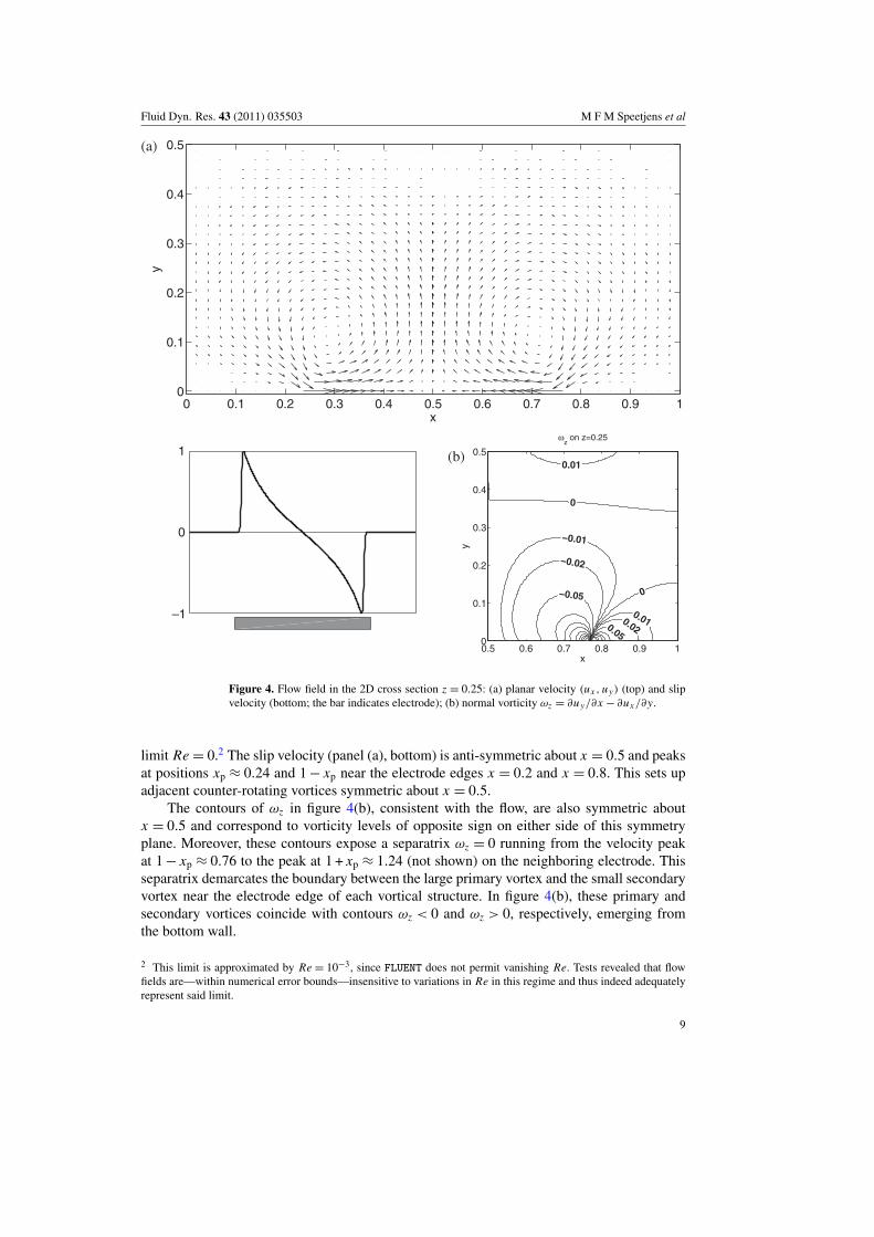
Figure 4. Flow field in the 2D cross section z = 0.25: (a) planar velocity (ux , u y) (top) and slipvelocity (bottom; the bar indicates electrode); (b) normal vorticity ωz = ∂u y/∂x − ∂ux/∂y.

limit Re = 0.2 The slip velocity (panel (a), bottom) is anti-symmetric about x = 0.5 and peaksat positions xp ≈ 0.24 and 1 − xp near the electrode edges x = 0.2 and x = 0.8. This sets upadjacent counter-rotating vortices symmetric about x = 0.5.

The contours of ωz in figure 4(b), consistent with the flow, are also symmetric aboutx = 0.5 and correspond to vorticity levels of opposite sign on either side of this symmetryplane. Moreover, these contours expose a separatrix ωz = 0 running from the velocity peakat 1 − xp ≈ 0.76 to the peak at 1 + xp ≈ 1.24 (not shown) on the neighboring electrode. Thisseparatrix demarcates the boundary between the large primary vortex and the small secondaryvortex near the electrode edge of each vortical structure. In figure 4(b), these primary andsecondary vortices coincide with contours ωz < 0 and ωz > 0, respectively, emerging fromthe bottom wall.

2 This limit is approximated by Re = 10−3, since FLUENT does not permit vanishing Re. Tests revealed that flowfields are—within numerical error bounds—insensitive to variations in Re in this regime and thus indeed adequatelyrepresent said limit.

9

Fluid Dyn. Res. 43 (2011) 035503 M F M Speetjens et al

0 0.2 0.4 0.6 0.8 1−1

−0.5

0

0.5

1

x

0.6

0.8

1 0 0.1 0.2 0.3 0.4 0.5

0

0.1

0.2

0.3

0.4

0.5

zx

y

(b)(a)

Figure 5. Flow topology for symmetric forcing in the non-inertial limit Re = 0: (a) electrodewisesymmetric slip velocity (heavy curve; dashed lines indicate symmetry axes; solid curve indicatesactual asymmetric slip velocity) and (b) 3D-closed streamlines in the interval 0.56 x 6 1.

The present ACEO flow resembles lid-driven flows in that fluid is set in motion by anonzero wall velocity. Examples relevant in this context are the 3D lid-driven flows consideredin various studies (Shankar 1997, 1998, Shankar and Deshpande 2000, Speetjens et al 2004,Speetjens et al 2006b). Here the steady translation of the rigid bottom wall causes an internalflow consisting, save for some weak and very localized corner vortices, of one vortex. Thereduced domain D∗ holds two counter-rotating vortices and thus basically comprises two suchlid-driven flows. The primary difference is that ACEO flows are driven by an x-dependentslip velocity according to figure 4(a) and thus in effect ‘feel’ an ‘elastic wall’. Hereafter it isdemonstrated that this is qualitatively inconsequential and relevant fundamental properties oflid-driven flows carry over to ACEO flows.

5.2. The role of (a)symmetry in the forcing

A fundamental property of said lid-driven flows is that symmetric flow forcing yields closedstreamlines in the non-inertial (Stokes) limit Re = 0 (Shankar 1997, 1998). The above analogyimplies that for the ACEO flow this situation must occur for the simplified momentumbalance

∇ p = ∇2u, (13)

in conjunction with a symmetric slip velocity for each vortex, i.e. within both intervals06 x 6 0.5 and 0.56 x 6 1. The presence of this property is investigated by imposing

〈uslip〉(x) = H ′(x) − H ′(x − 0.5) + H ′(x − 1), H ′(x) = 2H(x) − 1, (14)

with H(x) following section 4.2, as the non-constant symmetric counterpart to the above slipvelocity. Figure 5 gives 〈uslip〉 according to (14) in comparison to the actual asymmetric slipvelocity due to ACEO (indicated by heavy and solid curves, respectively, in panel (a); dashedlines indicate electrodewise symmetries) and demonstrates the resulting closed streamlines forRe = 0 by those occurring within the interval 0.56 x 6 1 (panel (b)). The streamline portraitin the interval 06 x 6 0.5 (not shown) is identical, yet with motion in the opposite direction.Thus two adjacent counter-rotating vortices are set up that are composed entirely of closedstreamlines similar to those shown in figure 5(b). This has the important ramification thatthis fundamental symmetry property, notwithstanding non-constant slip velocity, is indeed

10

Fluid Dyn. Res. 43 (2011) 035503 M F M Speetjens et al

0.5

1

0

0.50

0.5

zx

y

0 0.1 0.2 0.3 0.4 0.50

0.1

0.2

0.3

0.4

0.5

z

y

(a) (b)

Figure 6. Flow topology for asymmetric forcing in the non-inertial limit Re = 0: (a) torusdelineated by a single 3D streamline; (b) Poincaré section (plane x = 0.75). Dark markers indicatethe torus; bright markers indicate two neighboring tori.

retained by the ACEO flow. Moreover, this implies effectively 1D fluid motion and thus thelowest degree of disorder possible in a 3D flow.

The effect of asymmetry on the flow forcing is demonstrated in figure 6 for the flowfield due to the actual slip velocity. Figure 6(a) shows a typical streamline in the interval0.56 x 6 1 for Re = 0 that, together with their mirror images in the interval 06 x 6 0.5 (notshown), belongs to the two counter-rotating vortices above the electrode. The streamline isnon-closed and in that sense behaves consistently with the flow topology in 3D lid-drivenflows subject to asymmetric forcing (Shankar 1998, Shankar and Deshpande 2000). Furtherexamination by way of the Poincaré section with the plane x = 0.75 reveals that streamlinesdescribe concentric tori according to figure 6(b). Here dark and bright markers, respectively,indicate the streamline of figure 6(a) and two neighboring streamlines. (Note that the non-closedness of the two larger tori in the Poincaré section is a numerical effect. This is discussedin more detail in section 7.) Thus the flow topology has undergone a transformation inaccordance with the first Hamiltonian response scenario in section 3, namely coalescenceof closed streamlines into tori (here emerging as closed stream tubes). This, in turn, impliesthat asymmetry induces these scenarios and may thus be utilized for the manipulation of theflow topology and, inherently, transport properties.

5.3. The role of fluid inertia

Introducing fluid inertia in 3D steady lid-driven flows triggers the formation of tori andtheir subsequent (partial) Hamiltonian breakdown (section 3) (Shankar and Deshpande 2000,Speetjens et al 2006b). Figure 7 demonstrates that the tori in the non-inertial flow topologyin figure 6 undergo the same transition. Rational tori fall apart for sufficient fluid inertia (hereRe & 50) and give way to multiple families of tori embedded in chaotic bands; irrational torisurvive in a slightly deformed manner. Here the latter correspond to the inner tori closest to thecommon axis, as reflected in the persistence of the innermost torus and the inability of tracersemanating from outer tori to penetrate the ‘core region’ up to Re = 150. (Higher Re has notbeen examined.) This implies that the role of inertia, similar to that of asymmetry, also carriesover to ACEO flows. The tori emerging from breakdown of rational tori revolve about thecommon axis multiple times before reconnecting and thus appear as so-called ‘island chains’

11

Fluid Dyn. Res. 43 (2011) 035503 M F M Speetjens et al

0 0.1 0.2 0.3 0.4 0.50

0.1

0.2

0.3

0.4

0.5

z

y

Re=2

0 0.1 0.2 0.3 0.4 0.50

0.1

0.2

0.3

0.4

0.5

z

y

Re=10(a) (b)

0 0.1 0.2 0.3 0.4 0.50

0.1

0.2

0.3

0.4

0.5

z

y

Re=50

0 0.1 0.2 0.3 0.4 0.50

0.1

0.2

0.3

0.4

0.5

z

y

Re=75(c) (d)

0 0.1 0.2 0.3 0.4 0.50

0.1

0.2

0.3

0.4

0.5

z

y

Re=100

0 0.1 0.2 0.3 0.4 0.50

0.1

0.2

0.3

0.4

0.5

z

y

Re=150(e) (f)

Figure 7. Hamiltonian disintegration of the flow topology for asymmetric forcing due to fluidinertia. Shown are Poincaré sections (plane x = 0.75).

within ‘chaotic seas’. These tori and their ‘fingerprint’ in the Poincaré section are illustratedin figure 8 for Re = 50. The emergence and subsequent disintegration of island chains happenwithin the range 50. Re . 150 until basically only the core region has survived (figure 7(f)).Thus a state of nearly total chaos has been achieved.

12

Fluid Dyn. Res. 43 (2011) 035503 M F M Speetjens et al

0.5

1

0.05

0.350

0.5

zx

y

0.1 0.2 0.30

0.1

0.2

0.3

0.4

0.5

z

y

(a) (b)

Figure 8. New tori emerging from the breakdown of rational tori: (a) a single 3D streamlinedelineating a newly formed torus at Re = 50 and (b) the associated ‘island chain’ in the Poincarésection (plane x = 0.75).

The above findings reveal that fluid inertia has the same (qualitative) impact on theflow topology as asymmetric forcing in that both effects trigger the Hamiltonian responsescenarios following section 3. This is further substantiated by the inertia-induced coalescenceof the closed streamlines in figure 5 into basically the same tori as given in figure 6 (notshown). This implies that asymmetry and fluid inertia are (at least partially) interchangeablemeans by which to manipulate the flow topology. Both effects can namely be triggered by aproper electrode layout and actuation. Moreover, their impact can be amplified by concurrentintroduction, thus extending such control over the flow topology. The presence of tori in thenon-inertial limit for asymmetric forcing, instead of the closed streamlines in the symmetriccase, for example, gives the system a ‘head start’ in the inertia-induced progression towardglobal chaos (figure 7).

5.4. General topological make-up of the basic ACEO flow

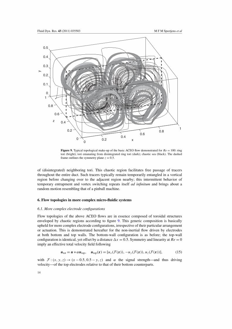
Each electrode sets up pairs of counter-rotating vortices within D∗. This, on account ofsymmetries (section 4.1), gives, within D, rise to symmetric arrangements of quadruples ofcoherent structures in the interval 06 x 6 1, demonstrated in figure 9 by way of the flowtopology for Re = 100 and an identical arrangement in the interval 16 x 6 2 (not shown).Shown are the elementary building blocks of Hamiltonian topologies: ring tori (bright); toriwith winding number higher than the one emanating from disintegrated ring tori (dark);chaotic sea (black).3 The symmetry plane z = 0.5 (dashed) acts as a transport barrier totracer migration and effectively divides the micro-channel into two disconnected parallelducts 06 z 6 0.5 and 0.56 z 6 1. Tracers within each duct are either entrapped within torior randomly wander around within the chaotic region formed by merger of chaotic seas

3 The winding number W represents the number of revolutions required for completing a full loop on a closed orbit.For the standard (or ‘ring’) torus W = 1; for tori formed by Hamiltonian breakdown generally W > 1.

13

Fluid Dyn. Res. 43 (2011) 035503 M F M Speetjens et al

00.2

0.40.6

0.81

0

0.2

0.4

0.6

0.8

10

0.1

0.2

0.3

0.4

0.5

x

z

y

Figure 9. Typical topological make-up of the basic ACEO flow demonstrated for Re = 100: ringtori (bright); tori emanating from disintegrated ring tori (dark); chaotic sea (black). The dashedframe outlines the symmetry plane z = 0.5.

of (disintegrated) neighboring tori. This chaotic region facilitates free passage of tracersthroughout the entire duct. Such tracers typically remain temporarily entangled in a vorticalregion before changing over to the adjacent region nearby; this intermittent behavior oftemporary entrapment and vortex switching repeats itself ad infinitum and brings about arandom motion resembling that of a pinball machine.

6. Flow topologies in more complex micro-fluidic systems

6.1. More complex electrode configurations

Flow topologies of the above ACEO flows are in essence composed of toroidal structuresenveloped by chaotic regions according to figure 9. This generic composition is basicallyupheld for more complex electrode configurations, irrespective of their particular arrangementor actuation. This is demonstrated hereafter for the non-inertial flow driven by electrodesat both bottom and top walls. The bottom-wall configuration is as before; the top-wallconfiguration is identical, yet offset by a distance 1x = 0.5. Symmetry and linearity at Re = 0imply an effective total velocity field following

utot = u + αutop, utop(x) = [ux (F(x)), −u y(F(x)), uz(F(x))], (15)

with F : (x, y, z) → (x − 0.5, 0.5 − y, z) and α the signal strength—and thus drivingvelocity—of the top electrodes relative to that of their bottom counterparts.

14

Fluid Dyn. Res. 43 (2011) 035503 M F M Speetjens et al

0

0.2

0.4

00.10.20.30.40.50

0.1

0.2

0.3

0.4

0.5

xz

y

0 0.1 0.2 0.3 0.4 0.50

0.1

0.2

0.3

0.4

0.5

z

y

(a) (b)

Figure 10. The formation of ring tori (bright) and toroidal structures comprising two truncated tori(dark) by top/bottom forcing (α = −0.2, Re = 0): (a) 3D streamlines delineating ring torus andtoroidal structure and (b) Poincaré section (x = 0.28).

Figure 10 shows the corresponding flow topology for α = −0.2 and reveals that theoriginal tori driven only by the bottom electrodes (α = 0; figure 6) partially survive (brightstreamline) and partially disintegrate in favor of newly formed tori at the top wall. Survivingsegments of the former and the emerging tori, both outlined by the dark streamlines infigure 10(a), define two families of tori ‘stacked’ vertically and truncated in localized chaoticregions near the wall z = 0 and the symmetry plane z = 0.5. These regions facilitate exchangeof material between both families of tori and thus give rise to random switching of fluid parcelsbetween an upper and a lower torus near z = 0 and conversely at z = 0.5. (The significant gapnear z = 0.5 in the Poincaré section in figure 10(b) illustrates this random jumping betweentori.) This manifests itself in a net circulation of material comprising alternating migrationtoward z = 0 and z = 0.5 through upper and lower tori, respectively, as demonstrated by thesingle dark streamline in figure 10(a). These randomly merged truncated tori effectively defineclosed toroidal structures that intertwine with the surviving original tori as two links of achain. It must be stressed that within said toroidal structures the Hamiltonian representationaccording to section 3 holds only piecewise within each truncated torus and breaks downlocally in the interconnecting chaotic regions.

Decreasing α results in further proliferation of the truncated tori at the expense of theoriginal ones until the latter have vanished completely for α = −1. Here truncated tori Temerge as discrete groups (T , T∗), with elements relating through the symmetry T∗ = F(T )

and F as before, and again randomly merge into complete toroidal structures accommodatingcirculatory fluid motion. This is demonstrated in figure 11 by way of two streamlines (brightand dark) that each delineate a different toroidal structure. Symmetry in the domain andelectrode layout causes reversal of the situation for α < −1 in that original tori re-emergeand truncated tori diminish, albeit arranged relative to the top electrodes and related to thetopology at −1 < α 6 0 via transformation F , until re-establishment of the single-wall statein the limit α → −∞.

Inertia causes Hamiltonian break-up in essentially the same way as demonstrated infigure 7. Electrode-wise symmetric forcing yields, similarly to figure 5, closed streamlines.Furthermore, here also x-wise merger of chaotic seas—and x-wise random tracer migration—as in figure 9 may happen. Asymmetry and inertia thus have an identical impact as before.Moreover, the shown tori are z-wise separated by the symmetry plane z = 0.5, again

15

Fluid Dyn. Res. 43 (2011) 035503 M F M Speetjens et al

0

0.2

0.4

00.10.20.30.40.50

0.1

0.2

0.3

0.4

0.5

xz

y

0 0.1 0.2 0.3 0.4 0.50.25

0.3

0.35

0.4

0.45

0.5

z

y

0 0.1 0.2 0.3 0.4 0.50

0.05

0.1

0.15

0.2

0.25

z

y

(a) (b)

Figure 11. The formation of concentric toroidal structures comprising two truncated tori bytop/bottom forcing (α = −1, Re = 0): (a) 3D streamlines delineating two toroidal structures(dark/bright) and (b) Poincaré sections at x = 0.2 (top) and x = 0.3 (bottom).

subdividing the micro-channel into disconnected parallel ducts. Hence, flow topologies ofgeneric ACEO flows are qualitatively analogous; more elaborate electrode configurationsmanifest themselves predominantly in a more complex arrangement of the same elementarybuilding blocks that admit systematic manipulation (within the bounds of Hamiltoniandynamics) by way of the actuation scenario of the electrodes in a way as demonstratedbefore. Spatiotemporal variation of ac signals may further extend the degree of control andflexibility (Ramos et al 2005, Squires 2009, Kim et al 2010). This, in principle, enableswide functionality, ranging from pumping via targeted (spatiotemporal) entrapment to mixing,within a given micro-system.

6.2. ACEO forcing in combination with other forcings

Functionality of micro-fluidic systems admits further expansion by combining ACEO forcingwith other forcings. This is demonstrated below for ACEO forcing by electrode pairs on thebottom walls in conjunction with axial forcing by a pressure gradient in the non-inertiallimit Re = 0. (This is equally representative of axial forcing due to electro-osmosis.) Thenon-inertial momentum balance admits linear decomposition of the total flow into the ACEOcomponent u and the pressure-driven component up following

utot = u + βup, (16)

with u as before and up = (ux , 0, 0) given by the Poiseuille flow

ux (y, z) =768

π4

∞∑m=1

∞∑n=1

[mn

(4m2 + n2

)]−1sin(2mπy) sin(nπ z), (17)

for ducts with rectangular cross-sections (Hunt 1965).4 The latter yields unit mean flow,meaning that the parameter β represents the ratio of characteristic axial to ACEO-driven

4 Solution (17) readily follows from the analytical solution for magnetohydrodynamics derived in Hunt (1965) ondisabling magnetic forcing.

16

Fluid Dyn. Res. 43 (2011) 035503 M F M Speetjens et al

0 0.2 0.4 0.6 0.8 1

0

0.1

0.2

0.3

0.4

0

0.1

0.2

0.3

0.4

0.5

xz

y

0 0.1 0.2 0.3 0.4 0.50

0.1

0.2

0.3

0.4

0.5

z

y

0 0.1 0.2 0.3 0.4 0.50

0.1

0.2

0.3

0.4

0.5

z

y

(a)

(b)

Figure 12. Flow topology due to combined ACEO and axial forcing (β = 0.01): (a) 3D streamlinesdelineating multiple families of tori (black/red) and disintegrating tori (cyan) and (b) Poincarésections at x = 0.25 (left) and x = 0.75 (right).

flows. Hence, growing β signifies diminishing ACEO-driven component and vice versa. Limitβ = 0 corresponds to pure ACEO flow and gives rise to electrode-wise quadruples of vorticessimilar to those shown in figure 9; limit → ∞ corresponds to purely axial flow. Augmentingaxial forcing by increasing β causes a transition from the former to the latter limit.

Non-zero axial flow (β > 0) introduces axial-wise symmetry breaking and thus bringsabout a fundamental change in topological make-up. This is demonstrated in figure 12 forβ = 0.01. The original tori partially survive in a slightly deformed manner (black). However,the outer tori associated with the electrode in the interval 06 x 6 0.5 ‘open up’ at their top

17

Fluid Dyn. Res. 43 (2011) 035503 M F M Speetjens et al

side in that their constituent streamlines are on the downstream side deflected toward theneighboring electrode, envelop the surviving tori in the interval 0.56 x 6 1 and subsequentlyreconnect with the remnants of said tori via the periodic inlet–outlet (cyan). This partialdisintegration of tori in fact underlies the formation of a common chaotic region reminiscentof that surrounding the tori in figure 9. Moreover, this results in the emergence of a familyof stream tubes connecting periodic inlet–outlet and constituting concentric serpentine-likechannels alternately running above and beneath surviving tori (red). These stream tubesare topologically equivalent to (disintegrated) tori in that tracers periodically return to thesame cross-section and, in consequence, exhibit the same dynamics as before. Hence, theyconstitute the tori of the first kind according to section 3 and are in fact hallmarks of theflow topology in axially driven duct flows (Speetjens et al 2006a). The coexistence of tori ofthe first and second kinds thus reflects the dual nature of the present flow in that it containselements of both vortical and uni-directional flows. Thus the present flow exhibits a richertopology than the purely ACEO-driven flows considered above.

Increasing the axial flow inflates the newly formed longitudinal tori and promotes furtherdisintegration of the original tori, as shown in figure 13 for β = 0.05. Here the original toriin the interval 0.56 x 6 1 also start to exhibit significant breakdown (blue). This processcontinues with growing β, as demonstrated in figure 14 for β = 0.1, causing diminutionof the original tori to confined areas near the side wall z = 0 (blue) and the bottom wall(black) and leading to the emergence of a second family of longitudinal tori (magenta)alongside the first one (red). Thus the flow topology gradually transforms into an intricatearrangement of multiple families of tori with various orientations and embedded in a commonchaotic sea. However, it remains composed of the same elementary building blocks as before,which is a direct consequence of the (region-wise) Hamiltonian structure of the equations ofmotion (section 3). Intermediate (chaotic) regions nonetheless seem to accommodate truly3D dynamics; local defects in tori appear to exist in the area pointed out by the arrow infigure 14(c) that facilitate random switching in a manner akin to that found before in thetruncated tori (section 6.1). Similar behavior has been observed in other 3D steady flows(Bajer and Moffatt 1990, Neishtadt and Vasiliev 1999).

The above analysis, together with that in section 6.1, demonstrates that ACEO forcing incombination with other forcing methods—principle—facilitates systematic creation of tailor-made flow topologies for the manifold transport challenges that arise in complex micro-fluidicsystems. Thus, ACEO flows (including other forcing) have the potential to afford a muchgreater functionality than mixing and pumping alone.

7. Performance of the numerical scheme

7.1. Introduction

The numerical scheme combines commercial CFD tools for the flow field with dedicatedalgorithms for the electrokinetic problem and Lagrangian trajectories. The motivation isthe attainment of maximal flexibility in geometry and boundary conditions—and ease ofuse.5 However, this ansatz typically yields less accuracy compared with dedicated software,meaning that their application and interpretation of results require appropriate care. Theinvestigation below addresses this issue by a performance analysis of the present numericalapproach regarding the resolution of fundamental topological properties.

5 Employment of a dedicated spectral solver for the electrokinetic problem (section 4.2) is non-essential here.A similar overall accuracy is reached upon resolving the entire system with standard CFD tools.

18

Fluid Dyn. Res. 43 (2011) 035503 M F M Speetjens et al

0 0.2 0.4 0.6 0.8 1

0

0.1

0.2

0.3

0.4

0

0.1

0.2

0.3

0.4

0.5

xz

y

0 0.1 0.2 0.3 0.4 0.50

0.1

0.2

0.3

0.4

0.5

z

y

0 0.1 0.2 0.3 0.4 0.50

0.1

0.2

0.3

0.4

0.5

z

y

(a)

(b)

Figure 13. Flow topology due to combined ACEO and axial forcing (β = 0.05): (a) 3D streamlinesdelineating multiple families of tori (black/red) and disintegrating tori (blue/cyan) and (b) Poincarésections at x = 0.25 (left) and x = 0.75 (right).

The Hamiltonian structure of the equations of motion leans solely on the continuityconstraint ∇ · u = 0 (Bajer 1994). Hence, its accurate approximation is of fundamentalimportance in that this largely determines the extent to which the Hamiltonian dynamics—andthe associated Lagrangian flow structure—can be reliably predicted by numerical simulations.Errors may emanate from the spatial discretization of the conservation laws (here FVM), thespatial interpolation of the flow field onto arbitrary positions and the time-marching schemefor the kinematic equation (6). Performance studies of standard FVM solvers against highlyaccurate dedicated spectral solvers exposed the limited approximation of continuity by theFVM solver as the primary cause for non-Hamiltonian (and thus non-physical) dynamics(Speetjens and Clercx 2005). Departures from continuity may manifest themselves in severalways and may thus serve as generic performance indicators.

19

Fluid Dyn. Res. 43 (2011) 035503 M F M Speetjens et al

0 0.2 0.4 0.6 0.8 1

0

0.1

0.2

0.3

0.4

0

0.1

0.2

0.3

0.4

0.5

xz

y

0 0.1 0.2 0.3 0.4 0.50

0.1

0.2

0.3

0.4

0.5

z

y

0 0.1 0.2 0.3 0.4 0.50

0.1

0.2

0.3

0.4

0.5

z

y

0 0.1 0.2 0.3 0.4 0.50

0.1

0.2

0.3

0.4

0.5

z

y

(a)

(b)

Figure 14. Flow topology due to combined ACEO and axial forcing (β = 0.1): (a) 3D streamlinesdelineating multiple families of tori (red/magenta) and disintegrating tori (black/blue/cyan),(b) Poincaré sections at x = 0.25 (left) and x = 0.75 (right) and (c) Poincaré section (x = 0.25)including additional 3D streamlines.

7.2. Resolution of fundamental topological properties

Symmetric forcing in the Stokes limit Re = 0 implies closed streamlines (section 5.2). Theformation of non-closed streamlines under such conditions is strong evidence of insufficientapproximation of continuity. This symmetry property is well resolved in the present study,as demonstrated in figure 5, where the gap between initial and final tracer positions aftercompletion of one revolution is of O(10−3) and remains in this range for subsequentrevolutions. Thus the employed numerical scheme adequately passes this first (yet essential)‘performance test’.

Hamiltonian dynamics dictate a specific topological response to perturbations (section 3).However, the preservation of this Hamiltonian nature is by far more challenging than theabove symmetry and, in a strict sense, even impossible. The reason for this is twofold.Firstly, disintegration of tori creates small-scale spatial features that greatly increase the

20

Fluid Dyn. Res. 43 (2011) 035503 M F M Speetjens et al

geometric complexity. Furthermore, this disintegration repeats itself ad infinitum within newlyformed features (Ottino 1989, Ott 2002), implying a cascade down to infinitesimally smallstructures, which, irrespective of resolution, a priori prohibits full capturing by any numericalmethod. Deviations from continuity are unavoidable for this phenomenon alone. Secondly,full demarcation of tori by 3D streamlines is a slow process—in particular for earlier stagesof the Hamiltonian progression, where secondary circulation is weak—and thus necessitatesnumerical tracking over large time intervals. (Tracking times easily exceed those for symmetryverification by several orders of magnitudes.) This amplifies approximation errors accordinglyand introduces further non-Hamiltonian effects.

The topological response to perturbation (here by fluid inertia) is demonstrated in figure 7.The shown response is fully consistent with Hamiltonian scenarios in that tori progressivelyfall apart into island chains and give way to chaos with stronger perturbation (growing Re).Note in particular the accurate demarcation of the island chains in figures 7(c)–(e), of whichthe 3D extents are given in figure 8. Hence, the simulated flow topology overall is physicallyvalid and adequately resolved by the numerical scheme. Non-Hamiltonian phenomena occuronly on a finer level in that 3D streamlines outlining tori emerge as non-closed orbits in thePoincaré sections. For irrational tori this results in a weakly spiralling motion about the trueclosed orbit (e.g. outer torus in figure 7(a)); for (nearly) rational tori, this typically causesconvergence of said streamlines on a fixed 3D curve, yielding a ‘fishhook’ pattern in thePoincaré section (e.g. the inner torus in figure 7(e)). These localized non-Hamiltonian effectshave also been found in other numerical studies using standard FVM/FEM schemes (Hobbsand Muzzio 1998, Shankar and Deshpande 2000, Speetjens and Clercx 2005, Speetjenset al 2006a) and must, for reasons given before, be taken for granted. The present schemenonetheless yields a degree of resolution that is perfectly adequate for general analysisand design purposes. The reliable isolation of the overall topological make-up of the morecomplex systems in section 6 and its consistency with Hamiltonian mechanics are a testamentto this. Suppression of said effects to very low levels is possible only with dedicatedhigher-order—and thus prohibitively expensive—numerical schemes (Speetjens andClercx 2005).

7.3. Computational effort

Tests exposed the resolution of the flow field by FLUENT as the main contribution to the totalcomputational effort. Simulations were run until residuals R of the mass and momentumbalances dropped below the preset upper bound Rmax = 10−12 (section 4.3). This was themaximum achievable degree of convergence and ensured the highest degree of approximationof—in particular—continuity. The attainment of this convergence in flows below Re ∼ 100typically required 45 000 iterations and 64 h simulation time using four parallel Intel Xeon2 GHz CPUs with 4 Gb memory. Resolution of the cases beyond Re ∼ 100 proved far morechallenging and demanded up to 275 000 iterations (taking about 390 h). This rise in effortstems from the growing complexity of the velocity field due to fluid inertia and increasinggradients by narrowing boundary layers. However, this is but a minor issue, since realisticmicro-flows rarely reach this regime.

8. Conclusions

The present study concerns the numerical simulation and analysis of the Lagrangianflow structure in ACEO micro-flows. This structure geometrically determines the transportproperties in essentially laminar flows such as e.g. micro-fluidics and thus insights into its

21

Fluid Dyn. Res. 43 (2011) 035503 M F M Speetjens et al

composition are of fundamental importance to systematic utilization of ACEO forcing formicro-mixers, micro-reactors and lab-on-a-chip applications. The analysis considers a basicperiodic micro-channel accommodating a 3D steady flow set up by ACEO forcing and insome cases including an axial background flow. Numerical simulations are performed by acombination of dedicated and commercially available CFD tools.

Incompressibility admits the (local) transformation of the 3D Lagrangian equations ofmotion into 2D non-autonomous Hamiltonian systems everywhere outside stagnation points.Thus, the present ACEO flows, save in the proximity of said points, in essence exhibitHamiltonian dynamics, which has fundamental ramifications for the flow topology. The keycoherent structures of Hamiltonian flow topologies are tori, which in the present class of 3Dsteady flows may emerge in two kinds: (i) stream tubes connecting the periodic inlet–outlet;(ii) closed stream tubes within the domain interior. These tori typically are in a (partial)state of disintegration due to perturbations induced by the flow forcing. This disintegrationfollows very specific Hamiltonian scenarios and results in the characteristic Hamiltoniantopology comprising (remnants of disintegrated) tori embedded in chaotic seas. This enablesa systematic strategy for transport studies.

The basic ACEO flow driven by electrodes on a single wall in essence resembles alid-driven flow in that fluid is set in motion by a wall velocity. Asymmetric driving velocityand fluid inertia both play an essential role in the topology of lid-driven flows by inducingthe formation of tori and determining their degree of disintegration. This study reveals thatthese fundamental properties carry over to the present ACEO flows. Moreover, it revealsthat fluid inertia has the same (qualitative) impact on the flow topology as asymmetricforcing, implying that they are (at least partially) interchangeable mechanisms that mayamplify one another. This offers a promising way for systematic manipulation of the flowtopology, since asymmetry and inertia are directly controlled by the forcing. ACEO forcing inparticular has great potential on the grounds of its flexibility in electrode layout and electrodeactuation.

The generic topological make-up of the basic ACEO flow is upheld for more complexACEO systems, including combination with other forcing, in that flow topologies remaincomposed of (multiple) families of tori embedded in (interconnected) chaotic seas. Theprimary manifestation of more elaborate electrode layout/actuation and introduction ofother forcing is a more complex arrangement of the same elementary building blocksthat admits systematic manipulation (within the bounds of Hamiltonian dynamics) byway of actuation scenario of the electrodes and relative strength of possible additionalforcing. This, in principle, facilitates the creation of tailor-made Lagrangian flow structuresfor various transport purposes, ranging from pumping via targeted (spatiotemporal)entrapment to mixing. This may greatly enhance the functionality and versatility of labs-on-a-chip.

Efficient numerical simulation of ACEO flows for various geometries and boundaryconditions necessitates commercial CFD tools. A key challenge with respect to Lagrangiantransport studies is sufficient approximation of the continuity constraint. Departures fromthis condition give rise to non-physical flow features. Important in this context is that fullresolution of the flow topology is strictly impossible due to the emergence of infinitesimallysmall structures by disintegration of tori that, inherently, defy any numerical approximation.Reliable isolation of the flow topology nonetheless is feasible with finite spatial resolutionand, provided sufficiently high, restricts non-Hamiltonian phenomena to localized small-scalefeatures. The most common effect is tori appearing non-closed due to slight deviation ofsimulated 3D streamlines from their true physical counterparts. However, this is immaterialfor general analysis and design purposes.

22

Fluid Dyn. Res. 43 (2011) 035503 M F M Speetjens et al

References

Aboelkassem Y 2010 Electroosmotic flow in a microchannel for microfluidic applications Eur. J. Sci. Res. 39 183Aref H 2002 The development of chaotic advection Phys. Fluids 14 1315Bajer K 1994 Hamiltonian formulation of the equations of streamlines in three-dimensional steady flows Chaos

Solitons Fractals 4 895Bajer K and Moffatt H K 1990 On a class of steady confined Stokes flows with chaotic streamlines J. Fluid Mech.

212 337Bazant M Z and Ben Y 2006 Theoretical prediction of fast 3D AC electro-osmotic pumps Lab Chip 6 1455Beebe D J, Mensing G A and Walker G M 2002 Physics and applications of microfluidics in biology Annu. Rev.

Biomed. Eng. 4 261Canuto C, Hussaini M Y, Quarteroni A and Zang T A 1988 Spectral Methods in Fluid Dynamics (Berlin: Springer)Cartwright J H E, Feingold M and Piro O 1996 Chaotic advection in three-dimensional unsteady incompressible

laminar flow J. Fluid Mech. 316 259Bertsch A, Heimgartner S, Cousseau P and Renaud P 2001 Static micromixers based on large-scale industrial mixer

geometry Lab on a Chip 1 56Chang C C and Yang R J 2004 Computational analysis of electrokinetically driven flow mixing in microchannels

with patterned blocks J. Micromech. Microeng. 14 550Chen J-K, Weng C-N and Yang R-J 2009 Assesment of three AC electroosmotic flow protocols for mixing in

microfluidic channel Lab on a Chip 9 1267Chen J L, Shih W H and Hsieh W H 2010 Three-dimensional non linear AC electro-osmotic flow induced by a

face-to-face, asymmetric pair of planar electrodes Microfluidics Nanofluidics 10 1007Funakoshi M 2008 Chaotic mixing and mixing efficiency in a short time Fluid Dyn. Res. 40 1Green N G, Ramos A, González A, Morgan H and Castellanos A 2002 Fluid flow induced by nonuniform AC electric

fields in elektrolytes on microelectrodes. III. Observation of streamlines and numerical simulation Phys. Rev. E66 26305

Hansen C and Quake S R 2003 Microfluidics in structural biology: smaller, faster . . . better Curr. Opin. Struct. Biol.13 538

Hobbs D M and Muzzio F J 1998 Optimization of a static mixer using dynamical systems techniques Chem. Eng.Sci. 53 3199

Hunt J C R 1965 Magnetohydrodynamic flow in rectangular ducts J. Fluid Mech. 21 577Khakhar D V, Franjione J G and Ottino J M 1987 A case study of chaotic mixing in deterministic flows: the

partitioned-pipe mixer Chem. Eng. Sci. 42 2909Kim D S, Lee I H, Kwon T H and Cho D W 2004 A barrier embedded kenics micromixer J. Micromech. Microeng.

14 1294Kim B J, Yoon S Y, Lee K H and Sung H J 2010 Development of a microfluidic device for simultaneous mixing and

pumping Exp. Fluids 46 85Kuo C-T and Liu C-H 2008 A novel microfluidic driver via AC electrokinetics Lab on a Chip 8 725Meagher R J, Hatch A V, Renzi R F and Singh A K 2008 An integrated microfluidic platform for sensitive and rapid

detection of biological toxins Lab on a Chip 8 2046Metcalfe G, Rudman M, Brydon A, Graham L and Hamilton R 2006 Composing chaos: an experimental and

computational study of an open duct mixing flow AIChE J. 52 9Meijer H E H, Singh M K, Kang T G, den Toonder J M J and Anderson P D 2009 Passive and active mixing in

microfluidic devices Macromol. Symp. 279 (Polymers at Frontiers of Science and Technology – MACRO 2008)201

Meisel I and Ehrhard P 2006 Electrically-excited (electroosmotic) flows in microchannels for mixing applicationsEur. J. Mech. B 25 491

Mills P L, Quiram D J and Ryley J F 2008 Microreactor technology and process miniaturization for catalyticreactions. A perspective on recent developments and emerging technologies Chem. Eng. Sci. 62 6992

Mizuno Y and Funakoshi M 2004 Chaotic mixing caused by an axially periodic steady flow in a partitioned-pipemixer Fluid Dyn. Res. 35 205

Neishtadt A I and Vasiliev A A 1999 Change of the adiabatic invariant at a separatrix in a volume-preserving3D system Nonlinearity 12 303

Nguyen N-T and Wu Z 2005 Micro-mixers—a review J. Micromech. Microeng. 15 R1Ott E 2002 Chaos in Dynamical Systems 2nd edn (Cambridge: Cambridge University Press)Ottino J M 1989 The Kinematics of Mixing: Stretching, Chaos and Transport (Cambridge: Cambridge University

Press)Ottino J M and Wiggins S 2004 Introduction: mixing in microfluidics Phil. Trans. R. Soc. A 362 923

23

Fluid Dyn. Res. 43 (2011) 035503 M F M Speetjens et al

Pacheco J R, Chen K P and Hayes M 2006 Efficient and rapid mixing in a slip-driven three-dimensional flow in arectangular channel Fluid Dyn. Res. 38 503–21

Pacheco J R, Chen K P, Pacheco-Vega A, Chen B and Hayes M A 2008 Chaotic mixing enhancement in electro-osmotic flows by random period modulation Phys. Lett. A 372 1001

Pearce T M and Williams J C 2007 Microtechnology: meet neurobiology Lab on a Chip 7 30Ramos A, Morgan H, Green N G, González A and Castellanos A 1999 AC electric-field-induced fluid flow in

microelectrodes J. Colloid Interface Sci. 217 420Ramos A, González A, Castellanos A, Green N G and Morgan H 2003 Pumping of liquids with AC voltages applied

to asymmetric pairs of microelectrodes Phys. Rev. E 67 056302Ramos A, Morgan H, Green N G, González A and Castellanos A 2005 Pumping of liquids with travelling–wave

electroosmosis J. Appl. Phys. 97 084906Shankar P N 1997 Three-dimensional eddy structure in a cylindrical container J. Fluid Mech. 342 97Shankar P N 1998 Three-dimensional Stokes flow in a cylindrical container Phys. Fluids 10 540Shankar P N and Deshpande M D 2000 Fluid mechanics in the driven cavity Annu. Rev. Fluid Mech. 32 93Speetjens M F M, Clercx H J H and van Heijst G J F 2004 A numerical and experimental study on advection in

three-dimensional Stokes flows J. Fluid Mech. 514 77Speetjens M F M and Clercx H J H 2005 A Spectral Solver for the Navier–Stokes equations in the velocity–vorticity

formulation Int. J. Comput. Fluid D 19 191Speetjens M, Metcalfe G and Rudman M 2006 Topological mixing study of non-Newtonian duct flows Phys. Fluids

18 103103Speetjens M F M, Clercx H J H and van Heijst G J F 2006 Merger of coherent structures in time-periodic viscous

flows Chaos 16 043104Squires T M 2009 Induced charge electrokinetics: fundamental challenges and opportunities Lab on a Chip 9 2477Stone H A, Stroock A D and Ajdari A 2004 Engineering flows in small devices: microfluidics toward a lab-on-a-chip

Annu. Rev. Fluid Mech. 36 381Tabeling P 2009 A brief introduction to slippage, droplets and mixing in microfluidic systems Lab on a Chip 9 2428Tourovskaia A, Figueroa-Masot X and Folch A 2005 Differentiation-on-a-chip: a microfluidic platform for long-term

cell culture studies Lab on a Chip 5 14Urbanski J P, Thorsen T, Levitan J A and Bazant M Z 2006 Fast AC electro-osmotic micropumps with nonplanar

electrodes Appl. Phys. Lett. 89 143508Urbanski J P, Levitan J A, Burch D N, Thorsen T and Bazant M Z 2007 The effect of step height on the performance

of three-dimensional AC electro-osmotic microfluidic pumps J. Colloid Interface Sci. 309 332Weigl B, Domingo G, Labarre P and Gerlach J 2008 Towards non- and minimally instrumented, microfluidics-based

diagnostic devices Lab on a Chip 8 1999Wiggins S and Ottino J M 2004 Foundations of chaotic mixing Phil. Trans. R. Soc. A 362 937

24