18 decision trees - CS CSU Homepagecs545/fall13/dokuwiki/lib/exe/fetch.php?media... · Decision Trees Chapter 5 1 Decision tree: an example 2 ... From the bottom: the relative size

11/11/13

1

Decision Trees

Chapter 5

1

Decision tree: an example

2

Example: classifying dolphins

Suppose we have a domain with the following positive and negative examples:

3

4. Concept learning 4.2 Paths through the hypothesis space

p.115 Example 4.4: Data that is not conjunctively separable I

Suppose we have the following five positive examples (the first three are thesame as in Example 4.1):

p1: Length= 3 ^ Gills= no ^ Beak= yes ^ Teeth=manyp2: Length= 4 ^ Gills= no ^ Beak= yes ^ Teeth=manyp3: Length= 3 ^ Gills= no ^ Beak= yes ^ Teeth= fewp4: Length= 5 ^ Gills= no ^ Beak= yes ^ Teeth=manyp5: Length= 5 ^ Gills= no ^ Beak= yes ^ Teeth= few

and the following negatives (the first one is the same as in Example 4.2):

n1: Length= 5 ^ Gills= yes ^ Beak= yes ^ Teeth=manyn2: Length= 4 ^ Gills= yes ^ Beak= yes ^ Teeth=manyn3: Length= 5 ^ Gills= yes ^ Beak= no ^ Teeth=manyn4: Length= 4 ^ Gills= yes ^ Beak= no ^ Teeth=manyn5: Length= 4 ^ Gills= no ^ Beak= yes ^ Teeth= few

Peter Flach (University of Bristol) Machine Learning: Making Sense of Data August 25, 2012 92 / 349

4. Concept learning 4.2 Paths through the hypothesis space

p.115 Example 4.4: Data that is not conjunctively separable I

Suppose we have the following five positive examples (the first three are thesame as in Example 4.1):

p1: Length= 3 ^ Gills= no ^ Beak= yes ^ Teeth=manyp2: Length= 4 ^ Gills= no ^ Beak= yes ^ Teeth=manyp3: Length= 3 ^ Gills= no ^ Beak= yes ^ Teeth= fewp4: Length= 5 ^ Gills= no ^ Beak= yes ^ Teeth=manyp5: Length= 5 ^ Gills= no ^ Beak= yes ^ Teeth= few

and the following negatives (the first one is the same as in Example 4.2):

n1: Length= 5 ^ Gills= yes ^ Beak= yes ^ Teeth=manyn2: Length= 4 ^ Gills= yes ^ Beak= yes ^ Teeth=manyn3: Length= 5 ^ Gills= yes ^ Beak= no ^ Teeth=manyn4: Length= 4 ^ Gills= yes ^ Beak= no ^ Teeth=manyn5: Length= 4 ^ Gills= no ^ Beak= yes ^ Teeth= few


5. Tree models

p.130 Figure 5.1: Paths as trees

Gills

Beak

=no

[0+, 4–]

=yes

Length

=yes

[0+, 0–]

=no

Teeth

=[3,5]

[1+, 1–]

≠[3,5]

Length

=few

[2+, 0–]

=many

[1+, 0–]

=3

[1+, 0–]

=5

ĉ(x) = ⊕

Gills

Length

=no

ĉ(x) = ⊖

=yes

Teeth

ĉ(x) = ⊖

=few

ĉ(x) = ⊕

=many

=3 =4

ĉ(x) = ⊕

=5

(left) The path from Figure 4.6, redrawn in the form of a tree. The coverage numbers inthe leaves are obtained from the data in Example 4.4. (right) A decision tree learned onthe same data. This tree separates the positives and negatives perfectly.


Figure 5.1

Decision tree

For now assume categorical data. Each internal node is labeled with a feature, and each edge is labeled with a value. Each leaf node is labeled with a class variable.

4

5. Tree models


Gills

Beak

=no

[0+, 4–]

=yes

Length

=yes

[0+, 0–]

=no

Teeth

=[3,5]

[1+, 1–]

≠[3,5]

Length

=few

[2+, 0–]

=many

[1+, 0–]

=3

[1+, 0–]

=5

ĉ(x) = ⊕

Gills

Length

=no

ĉ(x) = ⊖

=yes

Teeth

ĉ(x) = ⊖

=few

ĉ(x) = ⊕

=many

=3 =4

ĉ(x) = ⊕

=5



11/11/13

2

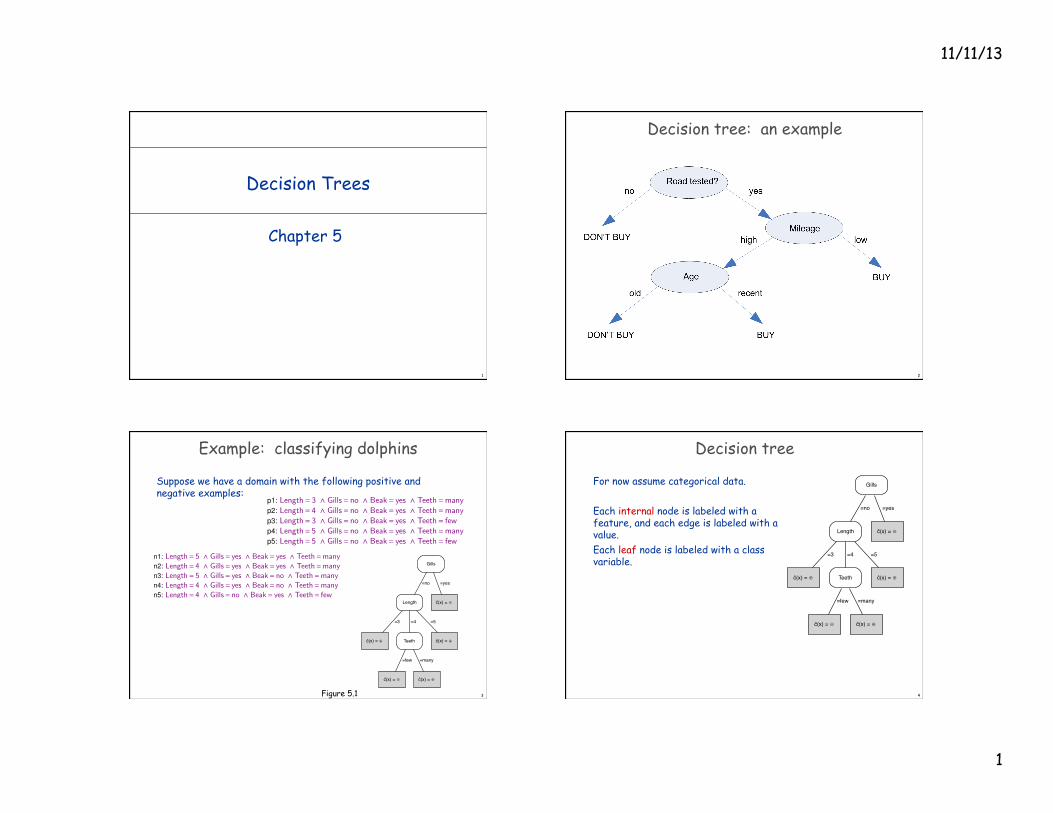
Splitting

5. Tree models 5.1 Decision trees

p.137 Figure 5.3: Decision tree for dolphins

D: [2+, 0−]

A: Gills

B: Length

=no

C: [0+, 4−]

=yes

E: Teeth

G: [0+, 1−]

=few

H: [1+, 0−]

=many

=3 =4

F: [2+, 0−]

=5

Negatives

Positives

p1,p3

p4-5

p1

n5 n1-4

AB

C

D

E

F

G

H

(left) Decision tree learned from the data in Example 4.4. (right) Each internal and leafnode of the tree corresponds to a line segment in coverage space: vertical segments forpure positive nodes, horizontal segments for pure negative nodes, and diagonalsegments for impure nodes.


5

Each node has a subset of the data associated with it

[5+, 5-]

[5+, 1-]

[1+, 1-]

Decision trees

Finding optimal decision tree is NP-hard. Rough idea: top down approach – at each step select the best attribute to perform a split on.

6

5. Tree models


Gills

Beak

=no

[0+, 4–]

=yes

Length

=yes

[0+, 0–]

=no

Teeth

=[3,5]

[1+, 1–]

≠[3,5]

Length

=few

[2+, 0–]

=many

[1+, 0–]

=3

[1+, 0–]

=5

ĉ(x) = ⊕

Gills

Length

=no

ĉ(x) = ⊖

=yes

Teeth

ĉ(x) = ⊖

=few

ĉ(x) = ⊕

=many

=3 =4

ĉ(x) = ⊕

=5


Peter Flach (University of Bristol) Machine Learning: Making Sense of Data August 25, 2012 100 / 349Learning decision trees

5. Tree models

p.132 Algorithm 5.1: Growing a feature tree

Algorithm GrowTree(D,F )

Input : data D ; set of features F .Output : feature tree T with labelled leaves.

1 if Homogeneous(D) then return Label(D) ; // Homogeneous, Label: see text2 S √BestSplit(D,F ) ; // e.g., BestSplit-Class (Algorithm 5.2)3 split D into subsets Di according to the literals in S;4 for each i do5 if Di 6=; then Ti √GrowTree(Di ,F ) else Ti is a leaf labelled with

Label(D);6 end7 return a tree whose root is labelled with S and whose children are Ti


7

5. Tree models

Growing a feature tree

Algorithm 5.1 gives the generic learning procedure common to most treelearners. It assumes that the following three functions are defined:

Homogeneous(D) returns true if the instances in D are homogeneous enoughto be labelled with a single label, and false otherwise;

Label(D) returns the most appropriate label for a set of instances D ;

BestSplit(D,F ) returns the best set of literals to be put at the root of the tree.

These functions depend on the task at hand: for instance, for classification tasksa set of instances is homogeneous if they are (mostly) of a single class, and themost appropriate label would be the majority class. For clustering tasks a set ofinstances is homogenous if they are close together, and the most appropriatelabel would be some exemplar such as the mean.


The best split method


p.137 Algorithm 5.2: Finding the best split for a decision tree

Algorithm BestSplit-Class(D,F )

Input : data D ; set of features F .Output : feature f to split on.

1 Imin √1;2 for each f 2 F do3 split D into subsets D1, . . . ,Dl according to the values v j of f ;4 if Imp({D1, . . . ,Dl }) < Imin then5 Imin √Imp({D1, . . . ,Dl });6 f

best

√ f ;7 end8 end9 return f

best


8

11/11/13

3

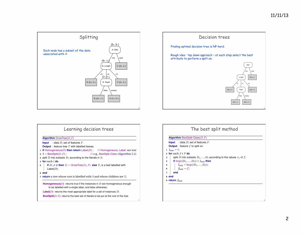
Node impurity

Given a feature and one of its values, a corresponding split divides the data D into subsets, D1,…, Dl, where l is the number of the feature Ideal situation: D1 contains all the positive or negative examples from D. This is a pure split. Notation: Pos/Neg number of pos/neg examples in D1 We will define impurity in terms of

p = Pos / (Pos + Neg) Desired properties from an impurity function: v  Maximal when p = ½ v  Minimal when p = 0 or p = 1 v  Symmetric in p, 1-p

9

Impurity functions


p.134 Figure 5.2: Measuring impurity

0 0.5 1

0.5

Imp(ṗ)

ṗ0

0.48

Gini index

ṗṗ1

ṗ2

(left) Impurity functions plotted against the empirical probability of the positive class.From the bottom: the relative size of the minority class, min(p,1° p); the Gini index,2p(1° p); entropy, °p log2 p ° (1° p) log2(1° p) (divided by 2 so that it reaches itsmaximum in the same point as the others); and the (rescaled) square root of the Giniindex,

pp(1° p) – notice that this last function describes a semi-circle. (right)

Geometric construction to determine the impurity of a split (Teeth= [many, few] fromExample 5.1): p is the empirical probability of the parent, and p1 and p2 are theempirical probabilities of the children.


10


p.134 Figure 5.2: Measuring impurity

0 0.5 1

0.5

Imp(ṗ)

ṗ0

0.48

Gini index

ṗṗ1

ṗ2

(left) Impurity functions plotted against the empirical probability of the positive class.From the bottom: the relative size of the minority class, min(p,1° p); the Gini index,2p(1° p); entropy, °p log2 p ° (1° p) log2(1° p) (divided by 2 so that it reaches itsmaximum in the same point as the others); and the (rescaled) square root of the Giniindex,

pp(1° p) – notice that this last function describes a semi-circle. (right)

Geometric construction to determine the impurity of a split (Teeth= [many, few] fromExample 5.1): p is the empirical probability of the parent, and p1 and p2 are theempirical probabilities of the children.


Digression: information theory

I am thinking of an integer between 0 and 1,023. You want to guess it using the fewest number of questions. Most of us would ask “is it between 0 and 512?” This is a good strategy because it provides the most information about the unknown number. It provides the first binary digit of the number. Initially you need to obtain log2(1024) = 10 bits of information. After the first question you only need log2(512) = 9 bits.

Information and Entropy

By halving the search space we obtained one bit. In general, the information associated with a probabilistic outcome: Why the logarithm? Assume we have two independent events x, and y. We would like the information they carry to be additive. Let’s check: The Entropy, or information associated with a random variable X: 12

I(p) = � log p

I(x, y) = � logP (x, y) = � logP (x)P (y)

= � logP (x)� logP (y) = I(x) + I(y)

Entropy(X) = �X

x

P (X = x) logP (X = x)

11/11/13

4

Entropy

For a Bernoulli random variable: Maximal when p = 1/2. A split is most informative when p=1 or p=0

Entropy(p) = �p log p� (1� p) log(1� p)5. Tree models 5.1 Decision trees

p.137 Figure 5.3: Decision tree for dolphins

D: [2+, 0−]

A: Gills

B: Length

=no

C: [0+, 4−]

=yes

E: Teeth

G: [0+, 1−]

=few

H: [1+, 0−]

=many

=3 =4

F: [2+, 0−]

=5

Negatives

Positives

p1,p3

p4-5

p1

n5 n1-4

AB

C

D

E

F

G

H

(left) Decision tree learned from the data in Example 4.4. (right) Each internal and leafnode of the tree corresponds to a line segment in coverage space: vertical segments forpure positive nodes, horizontal segments for pure negative nodes, and diagonalsegments for impure nodes.


[5+, 5-]

[5+, 1-]

[1+, 1-]

Impurity of a split

Given a feature and one of its values, a corresponding split divides the data D into subsets, D1,…, Dl, where l is the number of the feature i.e., the impurity of a split is the average impurity of the nodes

14

Imp({D1, . . . , Dl}) =lX

j=1

|Dj ||D| Imp(Dj )

Example


p.135 Example 5.1: Calculating impurity I

Consider again the data in Example 4.4. We want to find the best feature to putat the root of the decision tree. The four features available result in the followingsplits:

Length= [3,4,5] [2+,0°][1+,3°][2+,2°]Gills= [yes,no] [0+,4°][5+,1°]Beak= [yes,no] [5+,3°][0+,2°]Teeth= [many, few] [3+,4°][2+,1°]

Let’s calculate the impurity of the first split. We have three segments: the firstone is pure and so has entropy 0; the second one has entropy°(1/4) log2(1/4)° (3/4) log2(3/4) = 0.5+0.31 = 0.81; the third one has entropy1. The total entropy is then the weighted average of these, which is2/10 ·0+4/10 ·0.81+4/10 ·1 = 0.72.


15

Example 5. Tree models 5.1 Decision trees

p.135 Example 5.1: Calculating impurity II

Similar calculations for the other three features give the following entropies:

Gills 4/10 ·0+6/10 ·°°(5/6) log2(5/6)° (1/6) log2(1/6)

¢= 0.39;

Beak 8/10 ·°°(5/8) log2(5/8)° (3/8) log2(3/8)

¢+2/10 ·0 = 0.76;

Teeth 7/10 ·°°(3/7) log2(3/7)° (4/7) log2(4/7)

¢

+3/10·°°(2/3) log2(2/3)° (1/3) log2(1/3)

¢= 0.97.

We thus clearly see that ‘Gills’ is an excellent feature to split on; ‘Teeth’ is poor;and the other two are somewhere in between.The calculations for the Gini index are as follows (notice that these are on a scalefrom 0 to 0.5):

Length 2/10 ·2 · (2/2 ·0/2)+4/10 ·2 · (1/4 ·3/4)+4/10 ·2 · (2/4 ·2/4) = 0.35;Gills 4/10 ·0+6/10 ·2 · (5/6 ·1/6) = 0.17;Beak 8/10 ·2 · (5/8 ·3/8)+2/10 ·0 = 0.38;Teeth 7/10 ·2 · (3/7 ·4/7)+3/10 ·2 · (2/3 ·1/3) = 0.48.

As expected, the two impurity measures are in close agreement. See Figure 5.2(right) for a geometric illustration of the last calculation concerning ‘Teeth’.


16

11/11/13

5

Impurity of a split

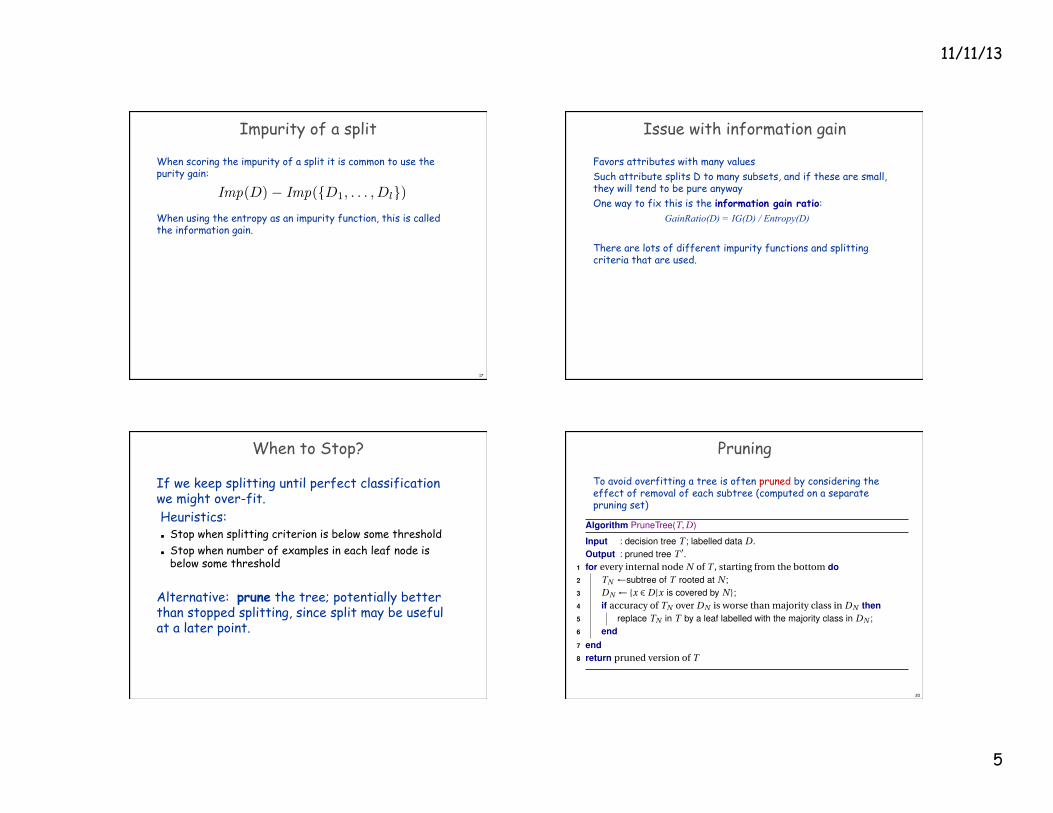
When scoring the impurity of a split it is common to use the purity gain: When using the entropy as an impurity function, this is called the information gain.

17

Imp(D)� Imp({D1, . . . , Dl})

Issue with information gain

Favors attributes with many values Such attribute splits D to many subsets, and if these are small, they will tend to be pure anyway One way to fix this is the information gain ratio:

GainRatio(D) = IG(D) / Entropy(D) There are lots of different impurity functions and splitting criteria that are used.

When to Stop?

If we keep splitting until perfect classification we might over-fit. Heuristics:   Stop when splitting criterion is below some threshold   Stop when number of examples in each leaf node is

below some threshold

Alternative: prune the tree; potentially better than stopped splitting, since split may be useful at a later point.

Pruning

To avoid overfitting a tree is often pruned by considering the effect of removal of each subtree (computed on a separate pruning set)

20

5. Tree models 5.2 Ranking and probability estimation trees

p.144 Algorithm 5.3: Reduced-error pruning

Algorithm PruneTree(T,D)

Input : decision tree T ; labelled data D .Output : pruned tree T 0.

1 for every internal node N of T , starting from the bottom do2 TN √subtree of T rooted at N ;3 DN √ {x 2 D|x is covered by N };4 if accuracy of TN over DN is worse than majority class in DN then5 replace TN in T by a leaf labelled with the majority class in DN ;6 end7 end8 return pruned version of T


11/11/13

6

Cost sensitivity of splitting criteria 5. Tree models 5.2 Ranking and probability estimation trees

p.144 Example 5.3: Skew sensitivity of splitting criteria I

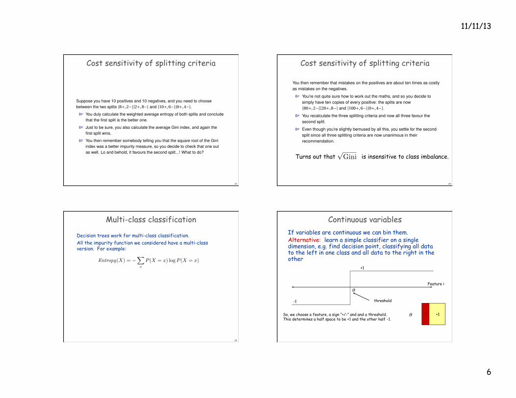
Suppose you have 10 positives and 10 negatives, and you need to choosebetween the two splits [8+,2°][2+,8°] and [10+,6°][0+,4°].

t You duly calculate the weighted average entropy of both splits and concludethat the first split is the better one.

t Just to be sure, you also calculate the average Gini index, and again thefirst split wins.

t You then remember somebody telling you that the square root of the Giniindex was a better impurity measure, so you decide to check that one outas well. Lo and behold, it favours the second split...! What to do?


Cost sensitivity of splitting criteria

22

5. Tree models 5.2 Ranking and probability estimation trees

p.144 Example 5.3: Skew sensitivity of splitting criteria II

You then remember that mistakes on the positives are about ten times as costlyas mistakes on the negatives.

t You’re not quite sure how to work out the maths, and so you decide tosimply have ten copies of every positive: the splits are now[80+,2°][20+,8°] and [100+,6°][0+,4°].

t You recalculate the three splitting criteria and now all three favour thesecond split.

t Even though you’re slightly bemused by all this, you settle for the secondsplit since all three splitting criteria are now unanimous in theirrecommendation.


pGiniTurns out that is insensitive to class imbalance.

Multi-class classification

Decision trees work for multi-class classification. All the impurity function we considered have a multi-class version. For example:

23

Entropy(X) = �X

x

P (X = x) logP (X = x)

Continuous variables If variables are continuous we can bin them. Alternative: learn a simple classifier on a single dimension, e.g. find decision point, classifying all data to the left in one class and all data to the right in the other

Feature i

threshold -1

+1

So, we choose a feature, a sign “+/-” and and a threshold. This determines a half space to be +1 and the other half -1.

θ -1 +1 -1

θ

11/11/13

7

Regression trees

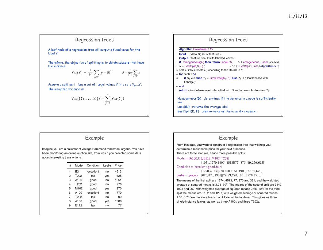
A leaf node of a regression tree will output a fixed value for the label Y. Therefore, the objective of splitting is to obtain subsets that have low variance. Assume a split partitions a set of target values Y into sets Y1,…,Yl. The weighted variance is:

25

Var(Y ) =1

|Y |X

y2Y

(y � y)2 y =1

|Y |X

y2Y

y

Var({Y1, . . . , Yl}) =lX

j=1

Var(Yj)

Regression trees

Homogeneous(D): determines if the variance in a node is sufficiently low Label(D): returns the average label BestSplit(D, F): uses variance as the impurity measure

26

5. Tree models

p.132 Algorithm 5.1: Growing a feature tree

Algorithm GrowTree(D,F )

Input : data D ; set of features F .Output : feature tree T with labelled leaves.

1 if Homogeneous(D) then return Label(D) ; // Homogeneous, Label: see text2 S √BestSplit(D,F ) ; // e.g., BestSplit-Class (Algorithm 5.2)3 split D into subsets Di according to the literals in S;4 for each i do5 if Di 6=; then Ti √GrowTree(Di ,F ) else Ti is a leaf labelled with

Label(D);6 end7 return a tree whose root is labelled with S and whose children are Ti


Example 5. Tree models 5.3 Tree learning as variance reduction

p.150 Example 5.4: Learning a regression tree I

Imagine you are a collector of vintage Hammond tonewheel organs. You havebeen monitoring an online auction site, from which you collected some dataabout interesting transactions:

# Model Condition Leslie Price

1. B3 excellent no 45132. T202 fair yes 6253. A100 good no 10514. T202 good no 2705. M102 good yes 8706. A100 excellent no 17707. T202 fair no 998. A100 good yes 19009. E112 fair no 77


Example

5. Tree models 5.3 Tree learning as variance reduction

p.150 Example 5.4: Learning a regression tree II

From this data, you want to construct a regression tree that will help youdetermine a reasonable price for your next purchase.There are three features, hence three possible splits:

Model= [A100,B3,E112,M102,T202][1051,1770,1900][4513][77][870][99,270,625]

Condition= [excellent,good, fair][1770,4513][270,870,1051,1900][77,99,625]

Leslie= [yes,no] [625,870,1900][77,99,270,1051,1770,4513]

The means of the first split are 1574, 4513, 77, 870 and 331, and the weightedaverage of squared means is 3.21 ·106. The means of the second split are 3142,1023 and 267, with weighted average of squared means 2.68 ·106; for the thirdsplit the means are 1132 and 1297, with weighted average of squared means1.55 ·106. We therefore branch on Model at the top level. This gives us threesingle-instance leaves, as well as three A100s and three T202s.


28

11/11/13

8

Example 5. Tree models 5.3 Tree learning as variance reduction

p.150 Example 5.4: Learning a regression tree III

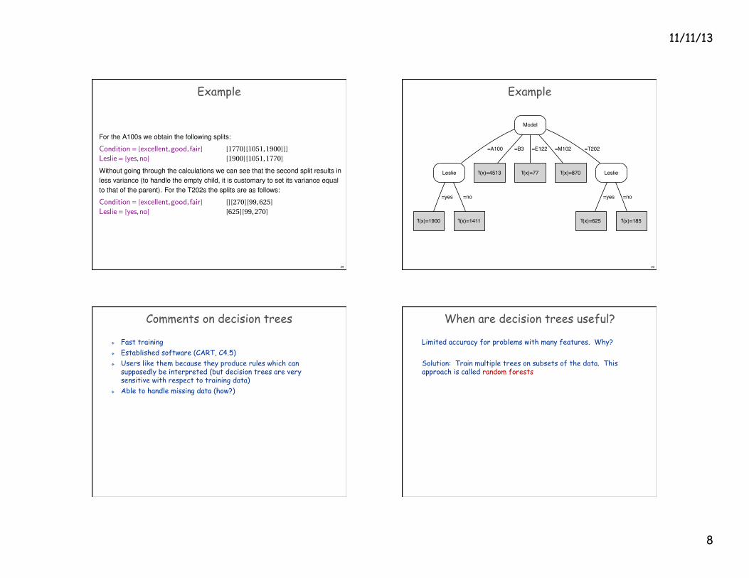
For the A100s we obtain the following splits:

Condition= [excellent,good, fair] [1770][1051,1900][]Leslie= [yes,no] [1900][1051,1770]

Without going through the calculations we can see that the second split results inless variance (to handle the empty child, it is customary to set its variance equalto that of the parent). For the T202s the splits are as follows:

Condition= [excellent,good, fair] [][270][99,625]Leslie= [yes,no] [625][99,270]

Again we see that splitting on Leslie gives tighter clusters of values. The learnedregression tree is depicted in Figure 5.8.


29

Example

5. Tree models 5.3 Tree learning as variance reduction

p.150 Figure 5.8: A regression tree

Model

Leslie

=A100

f(x)=4513

=B3

f(x)=77

=E122

f(x)=870

=M102

Leslie

=T202

f(x)=1900

=yes

f(x)=1411

=no

f(x)=625

=yes

f(x)=185

=no

A regression tree learned from the data in Example 5.4.


30

Comments on decision trees

v  Fast training v  Established software (CART, C4.5) v  Users like them because they produce rules which can

supposedly be interpreted (but decision trees are very sensitive with respect to training data)

v  Able to handle missing data (how?)

When are decision trees useful?

Limited accuracy for problems with many features. Why? Solution: Train multiple trees on subsets of the data. This approach is called random forests

Documents

18 decision trees - CS CSU Homepagecs545/fall13/dokuwiki/lib/exe/fetch.php?media... · Decision Trees Chapter 5 1 Decision tree: an example 2 ... From the bottom: the relative size