1

Except for reformatting and the addition of a reference list, the authors believe that this MS does not differ from that published as: Hutchinson, J. M. C., Fanselow, C. & Todd, P. M. (2012). Car parking as a game between simple heuristics. Pp. 454–484 in P.M. Todd, G. Gigerenzer & The ABC Research Group (Eds), Ecological rationality: intelligence in the world. New York: Oxford University Press

_____________________

18

Car Parking as a Game Between Simple Heuristics

John M. C. Hutchinson

Carola Fanselow

Peter M. Todd

The road to success is lined with many tempting parking spaces.

Anonymous

You are driving into town looking for somewhere to park. There seem not to be many parking spaces available at this time of day, and the closer you get to your destination, the fewer vacancies there are. After encountering a long stretch without a single vacancy, you fear that you have left it too late and are pleased to take the next place available—but then somewhat annoyed when completing the journey on foot to find many vacancies right next to your destination. Evidently everyone else had also assumed that the best spots must have been taken and had parked before checking them. Something to remember for next time: Given the pessimistic habits of others maybe it would be better to try a different strategy by driving straight to the destination and then searching outward.

For many of us, looking for a good parking space is a very familiar problem, and we probably expend some mental effort not to be too inefficient at it, especially in the rain or when we expect to carry a load back to our car. However, finding the best parking space can never be guaranteed because we lack full information of the spaces and competitors ahead. Moreover, even if our ambition is merely to make the best decision on average from the information available, the quantity and diversity of this information (parking patterns already observed, time of day, number of other drivers, etc.) suggest that processing it optimally is too complex for our cognitive capabilities. Various authors have come to a similar conclusion. As van der Goot (1982, p. 109) put it, “There is every reason to doubt whether the choice of a parking place is (always) preceded by a conscious and rational process of weighing the various possibilities.” In his book Traffic, Vanderbilt (2008, p. 146) noted that with regard to foraging for food or for parking, “neither animals nor humans always follow optimal strategies,” owing to cognitive limitations.

Instead, we envisage that drivers typically use fairly simple heuristics (rules of thumb) to make good decisions, if not the best possible ones, about where and when to park. An example could be, “If I have not found a space in the last 5 minutes, take the next one I encounter.” As we have seen throughout this book, there are many other decision domains in which simple heuristics have been found that can perform about as well as more complex solutions, by taking advantage of the available structures of information in the decision environment. Furthermore, these heuristics often generalize to new situations better than do complex strategies, because they avoid overfitting (see

2

chapter 2). Could simple rules also be successful at the task of finding a good parking space? And what features of the parking environment, itself shaped by the decisions of drivers seeking a space, might such rules exploit to guide us to better choices? These are the questions we explore in this chapter.

Selecting a parking space belongs to the class of sequential search problems, for which some successful heuristics have already been explored in the literature. These problems crop up in many different domains, whenever choices must be made between opportunities that arise more-or-less one at a time; in particularly challenging (and realistic) cases the qualities of future opportunities are unpredictable and returning to an opportunity that arose earlier is costly or impossible. Thus, decisions about each opportunity must be made on the spot: Should I accept this option, or reject it and keep searching for a better one? This decision can depend on the memory of the qualities of past opportunities, for instance by using those qualities to set an aspiration level to guide further search (Herbert Simon’s notion of satisficing search—see Simon, 1955a). One familiar, and well investigated, example of sequential search is mate search (e.g., Hutchinson & Halupka, 2004; Todd & Miller, 1999; Wiegmann & Morris, 2005). Another example, which also might have been familiar to our ancestors, is deciding at which potential campsite to stop for the night when on a journey through unfamiliar territory. Simple heuristics that work well, and that people use, have been studied in a number of sequential search settings (Dudey & Todd, 2002; Hey, 1982; Martin & Moon, 1992; Seale & Rapoport, 1997, 2000). The search for a parking space is a version of such sequential decision making: Parking spaces are encountered one at a time and must be decided upon when they are found in ignorance of whether better spaces lie ahead; moreover, they are often unavailable to return to later because other drivers may have filled them up.

It seems plausible that heuristics that work well in one sequential-search domain will work well in another. If evolution has adapted our heuristics in domains such as mate choice, we might tend to apply similar heuristics in novel sequential-search contexts such as selecting a house or parking a car. We might also have the ability to invent new heuristics for novel situations, but those that prove satisfactory may be the same ones as used in other sequential-choice problems. In either case, good candidates for parking heuristics might be those already proposed for other sequential search problems, so we will begin our exploration with a set of such strategies.

There are several reasons why car parking provides a particularly tractable example of sequential search to model and test empirically. One advantage is that it seems reasonable in many cases to quantify parking-site quality simply as the distance from one’s destination, whereas in other domains, such as mate search, quality is often multidimensional, difficult to measure, and not ranked consistently by different individuals. Another advantage is that once a car is parked the decision making is over, avoiding the complications of multiple and reversible decisions that occur in some other domains such as mate choice. Furthermore, parking decisions take place over an easily observable time scale. And because car parking is a problem that many people encounter repeatedly, they have the possibility to adapt the parameters of any heuristic they use to the environment encountered. This improves the chance that empirical observations will match predictions made assuming individuals maximize their performance—the predictions from the computer simulations in this chapter are based on this assumption.

The world of parking has another aspect that motivated us to work on this problem—the pattern of available and filled parking places is not generated by randomly sprinkling cars across a parking lot but rather is created through the decisions of the drivers who parked earlier. It thus provides a familiar simple example of an important class of problems in which critical aspects of the environment are constructed by the other players. Our goal is to find which heuristics work well for choosing parking places in the environment (pattern of vacant spaces) created by the heuristics used by others. Because we expect the heuristics used by others also to have been chosen to work well against their competitors, we arrive in the world of game theory. In game theory the usual approach is to search for equilibria. At equilibrium the distribution of strategies in the population is such that any driver cannot improve performance by choosing a different strategy, so there is no incentive to change strategy. Consequently, populations that reach these equilibria should remain on them and

3

thus such equilibria are what we generally expect to observe.1 Note that we are not envisaging that drivers use introspection to calculate which strategies will lead to equilibria, but rather that through trial and error and simple learning rules they discard poorly performing strategies and come to use those that work well.2

In this chapter we describe our search for decision strategy equilibria in an agent-based model that simulates drivers making parking decisions along an idealized road. By investigating equilibria, we sought strategies that work well against each other in the social environments that they themselves create. We begin by considering past work on parking and other forms of sequential search, then describe our model and the equilibria that emerge both when all drivers must use the same strategy and in the more realistic setting when we allow drivers to differ in the ways they search. Given the similarities between parking search and other forms of search mentioned earlier, results from the parking domain may be informative about other sequential-search domains, but here we concentrate on just the single domain, demonstrating an approach to exploring ecological rationality in situations where agents shape their own environments.

Previous Work on Parking Strategies

Curiously, the strategic game-theoretic aspect of the parking problem seems to have been largely neglected in earlier studies of car parking. Most have assumed a randomly produced pattern of available spaces at some constant density, patently different from the situations real drivers encounter. In one of the few analyses to consider the patterns created by drivers parking, Anderson and de Palma (2004) explored the equilibrium occupancy of parking places in a situation similar to ours, with the aim of devising pricing for parking that would alleviate congestion near the destination. However, they assumed that parking search “can be described by a stochastic process with replacement” (p. 5) in which drivers check the availability of spots at random and forget if they have checked one before, which is very different from the plausible search process that we consider. An earlier model of the effects of pricing by Arnott and Rowse (1999) had drivers use a decision rule based on their distance from the destination (the fixed-distance heuristic that we describe later) and assumed independence of neighboring parking spaces (which they note is an approximation)—but the nonindependent pattern of spaces created by other drivers is exactly the kind of structure that we want to investigate.

The problem of determining good strategies for finding a parking place has also been addressed within the more abstract mathematical framework of optimal stopping problems (DeGroot, 1970). In the original formulation of what was called the “Parking Problem” (MacQueen & Miller, 1960), drivers proceed down an endless street toward a destination somewhere along that street, passing parking places that are occupied with some constant probability p, and they must choose a space that minimizes the distance from the destination (either before or after it). The optimal strategy in this case is a threshold rule that takes the first vacancy encountered after coming within r parking places of the destination, where r depends on the density p of occupied parking places. For instance, if p = .9, then r = 6, while if p ≤ .5, then r = 0 (i.e., you should drive all the way to the destination and start looking for a space beyond; Ferguson, n.d., p. 2.11). This optimal solution provides a useful comparison for our simulations. However, in this original Parking Problem parking places are filled randomly so that the probability of one being occupied is independent of its location or of whether neighboring places are occupied. Besides not assuming such independence, our scenario also differs in that we mostly use a dead-end rather than infinite road, and we consider performance

1. However, such equilibria need not exist, and environmental fluctuations can lead to them not being attained. Also, if several theoretical equilibria exist, it can be difficult to predict which of them will be occupied in a real setting.

2. Both these processes of introspection and learning normally lead to the same equilibria (e.g., Kreps 1990, chapter 6), but we believe that economists and psychologists have tended to overemphasize the use of introspection in everyday (as opposed to novel experimental) situations.

4

criteria other than just parking distance from the destination. Other mathematical analyses of extensions of the parking problem have considered various complications (e.g., allowing drivers to turn around at any point—Tamaki, 1988—and varying the probability of occupancy as a function of distance from the destination—Tamaki, 1985), but not in ways that address the game-theoretic aspects that we focus on.

Experimental investigations of heuristics used by people for more abstract sequential search problems have been carried out by Seale and Rapoport (1997, 2000). They studied the classic secretary problem, in which people see a sequence of numbers (or their ranks) one at a time and try to select the highest value, without being able to return to any previously seen value. They investigated three types of rule: cutoff rules, which check a fixed proportion of the available options and then take the first option thereafter that is better than all those previously seen; candidate count rules, which stop on the nth candidate seen, where a candidate is an option that is better than all options previously encountered; and successive non-candidate count rules, which count up the number of values seen since the previous candidate and stop at the next candidate after that count has exceeded some threshold. By testing these rules with different parameter values in simulation and experiments, Seale and Rapoport found that cutoff rules perform best (they are optimal under some assumptions) and are most often used by people in experiments. Successive non-candidate count rules came close in performance, but candidate count rules fared poorly. Dudey and Todd (2002) considered how these rules performed in the task of maximizing expected quality (rather than maximizing the chance of finding the highest quality individual from a set) and found the same relative performances. In addition, when environments changed by getting better over time (e.g., when the distribution from which encountered options are drawn shifts upward with successive options), cutoff rules continued to perform best; this situation corresponds roughly to the parking situation we consider here, where drivers encounter a sequence of spaces that by definition improve the closer they get to their destination. (See Bearden & Connolly, 2007, and Lee, 2006, for empirical and theoretical extensions of the sequential search problem.)

Hutchinson and Halupka (2004) compared the performance of various heuristics in a somewhat different sequential choice scenario based on mate choice. The cutoff and candidate count rules performed much worse than heuristics in which males choose the first female who exceeds a fixed quality threshold (or one from a sequence of declining thresholds). The values of these thresholds were envisaged to have evolved in response to the distributions of mate qualities encountered by the population in earlier years. Likewise with parking, drivers may well know from experience the likely distribution of “qualities” available (certainly this is the assumption of our game-theoretic analysis), so it could again be true that fixed thresholds perform well.

Modeling the Interaction of Parking Strategies

To investigate the performance and equilibria of parking heuristics in different environments, we set up an agent-based model in which drivers follow various heuristics as they drive along a road searching for a good parking space. In this section we describe the fixed aspects of the environment in which parking takes place, including its physical layout and some social factors such as the flux of arriving cars.

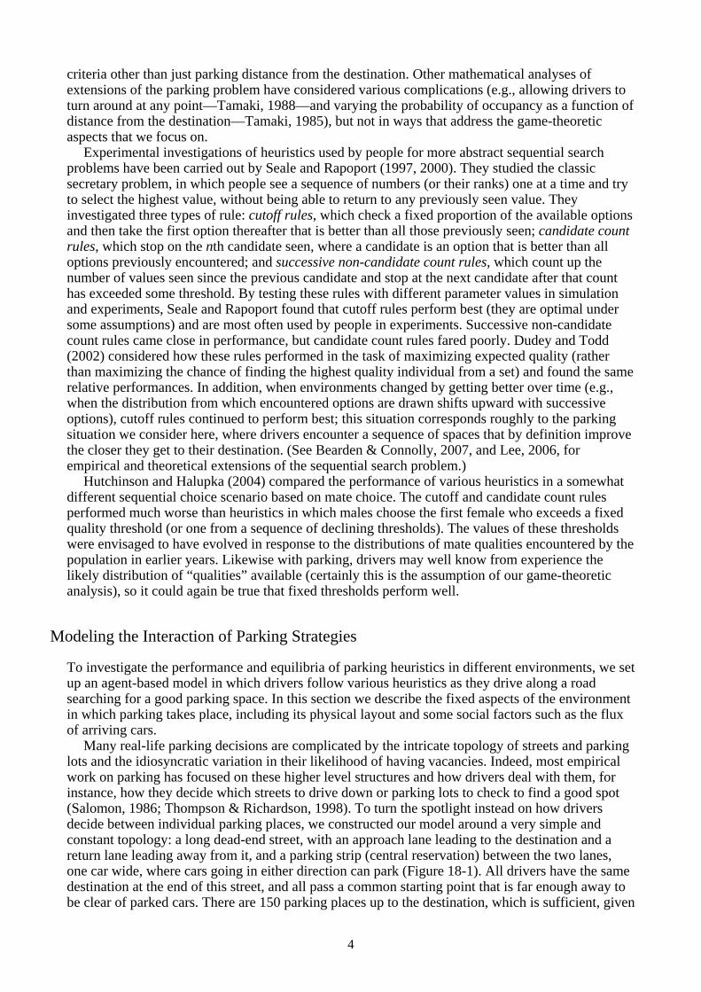
Many real-life parking decisions are complicated by the intricate topology of streets and parking lots and the idiosyncratic variation in their likelihood of having vacancies. Indeed, most empirical work on parking has focused on these higher level structures and how drivers deal with them, for instance, how they decide which streets to drive down or parking lots to check to find a good spot (Salomon, 1986; Thompson & Richardson, 1998). To turn the spotlight instead on how drivers decide between individual parking places, we constructed our model around a very simple and constant topology: a long dead-end street, with an approach lane leading to the destination and a return lane leading away from it, and a parking strip (central reservation) between the two lanes, one car wide, where cars going in either direction can park (Figure 18-1). All drivers have the same destination at the end of this street, and all pass a common starting point that is far enough away to be clear of parked cars. There are 150 parking places up to the destination, which is sufficient, given

5

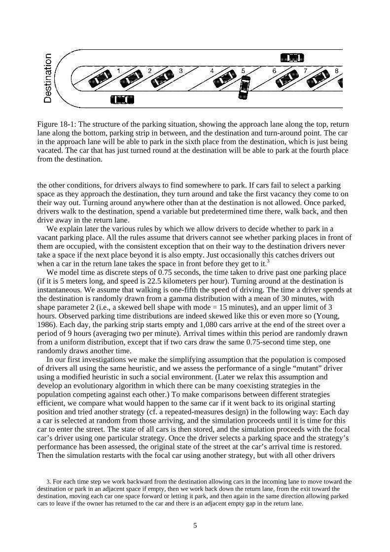
Figure 18-1: The structure of the parking situation, showing the approach lane along the top, return lane along the bottom, parking strip in between, and the destination and turn-around point. The car in the approach lane will be able to park in the sixth place from the destination, which is just being vacated. The car that has just turned round at the destination will be able to park at the fourth place from the destination. the other conditions, for drivers always to find somewhere to park. If cars fail to select a parking space as they approach the destination, they turn around and take the first vacancy they come to on their way out. Turning around anywhere other than at the destination is not allowed. Once parked, drivers walk to the destination, spend a variable but predetermined time there, walk back, and then drive away in the return lane.

We explain later the various rules by which we allow drivers to decide whether to park in a vacant parking place. All the rules assume that drivers cannot see whether parking places in front of them are occupied, with the consistent exception that on their way to the destination drivers never take a space if the next place beyond it is also empty. Just occasionally this catches drivers out when a car in the return lane takes the space in front before they get to it.3

We model time as discrete steps of 0.75 seconds, the time taken to drive past one parking place (if it is 5 meters long, and speed is 22.5 kilometers per hour). Turning around at the destination is instantaneous. We assume that walking is one-fifth the speed of driving. The time a driver spends at the destination is randomly drawn from a gamma distribution with a mean of 30 minutes, with shape parameter 2 (i.e., a skewed bell shape with mode = 15 minutes), and an upper limit of 3 hours. Observed parking time distributions are indeed skewed like this or even more so (Young, 1986). Each day, the parking strip starts empty and 1,080 cars arrive at the end of the street over a period of 9 hours (averaging two per minute). Arrival times within this period are randomly drawn from a uniform distribution, except that if two cars draw the same 0.75-second time step, one randomly draws another time.

In our first investigations we make the simplifying assumption that the population is composed of drivers all using the same heuristic, and we assess the performance of a single “mutant” driver using a modified heuristic in such a social environment. (Later we relax this assumption and develop an evolutionary algorithm in which there can be many coexisting strategies in the population competing against each other.) To make comparisons between different strategies efficient, we compare what would happen to the same car if it went back to its original starting position and tried another strategy (cf. a repeated-measures design) in the following way: Each day a car is selected at random from those arriving, and the simulation proceeds until it is time for this car to enter the street. The state of all cars is then stored, and the simulation proceeds with the focal car’s driver using one particular strategy. Once the driver selects a parking space and the strategy’s performance has been assessed, the original state of the street at the car’s arrival time is restored. Then the simulation restarts with the focal car using another strategy, but with all other drivers

3. For each time step we work backward from the destination allowing cars in the incoming lane to move toward the destination or park in an adjacent space if empty, then we work back down the return lane, from the exit toward the destination, moving each car one space forward or letting it park, and then again in the same direction allowing parked cars to leave if the owner has returned to the car and there is an adjacent empty gap in the return lane.

6

arriving at the same times, spending the same times at the destination and using the same strategies as before. Our comparisons of strategies were typically based on means of 100,000 focal cars.4

A Nash Equilibrium for a Simple Satisficing Strategy

Our main aim is to understand which parking strategies are ecologically rational. This requires specifying the environment, which is strongly shaped by the strategies used by other parkers. In this section we investigate the dependence of a driver’s parking performance on the strategies used by that driver and by other drivers and use these results to calculate how the population strategy would evolve if all drivers select strategies that increase their performance. For ease of illustration, we will consider in this section only the very simple fixed-distance heuristic that ignores all spaces until the car reaches D places from the destination and then takes the first vacancy (unless, as always, there is another vacancy immediately ahead). This is a form of satisficing with parameter D defining the aspiration level.

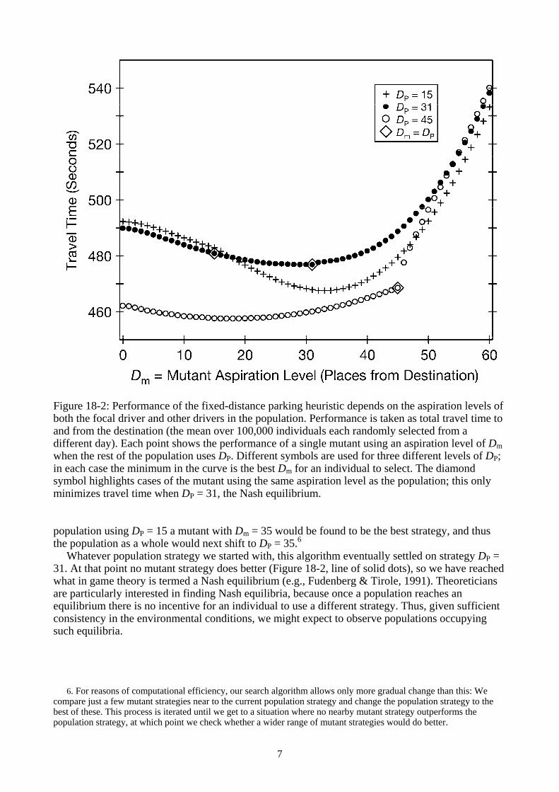
We first ask how well one driver does by changing strategy while the rest of the population uses the fixed-distance strategy with an aspiration level fixed at DP (the population parameter). Each simulation day we calculated the performance of a driver who uses the same fixed-distance strategy but with different mutant values of the parameter (Dm). The open circles in Figure 18-2 show how the mutant strategies performed as we changed Dm when the population was using DP = 45. Performance is here assessed in terms of total travel time, including time to drive to and from the parking place and walk to and from the destination, so lower values indicate better performance.5

One conspicuous feature of the graph is the sudden deterioration in performance if the mutant driver accepts a place farther from the destination than everybody else does. The reason is that there is often a vacancy 46 places from the destination that everybody else (using DP = 45) has ignored; a mutant using Dm = 46 is thus quite likely to end up there and perform much worse than the population average. (The same is true of mutants using larger values of Dm.) There is thus a considerable advantage in holding out as long as everybody else, but it matters less how much closer to the destination one’s threshold is (i.e., how much lower Dm is than DP). If the mutant instead uses Dm = 44, there probably will not be another vacancy for some distance (because spaces in this region would have been taken by other members of the population). In fact, the next available space, say at position K, would also be the one taken by mutants with values of Dm between DP and K, so those mutant strategies will therefore have similar levels of performance to Dm = 44 (as shown by the flattening of the line of open circles). If we change the population’s value of DP by a few places the position of the kink in the graph shifts correspondingly.

The line of crosses in Figure 18-2 shows the outcome when the population strategy shifts more dramatically to DP = 15. The kink has disappeared and the mutant driver now does better to accept a space farther from the destination than would the rest of the population. This is because if it seeks only a closer space (Dm < 15), it will probably not find one on the way to the destination and will thus waste time driving there and back before taking one farther than 15 parking places from the destination; this probably was already available on the inward journey. In this social environment (DP = 15) it is better for the mutant to take Dm = 45 than Dm = 15, whereas in the other social environment (DP = 45) the converse was true. Is there a stable equilibrium strategy between these two points where it pays to be exactly as picky as the rest of the population?

To find out, we proceeded through a succession of steps in which the population strategy always shifts to the strategy of the most successful mutant tested in the previous step. So for instance, in a

4. A different procedure was used to compare situations in which every individual in the population uses the same strategy. For each day we recorded the performance of every car and took the average. We then averaged this average over 100,000 days of independent simulations.

5. More precisely, the vertical axis measures the time from arriving at a starting position 150 spaces from the destination until returning to this starting position on the way back, but omitting the time spent at the destination itself.

7

Figure 18-2: Performance of the fixed-distance parking heuristic depends on the aspiration levels of both the focal driver and other drivers in the population. Performance is taken as total travel time to and from the destination (the mean over 100,000 individuals each randomly selected from a different day). Each point shows the performance of a single mutant using an aspiration level of Dm when the rest of the population uses DP. Different symbols are used for three different levels of DP; in each case the minimum in the curve is the best Dm for an individual to select. The diamond symbol highlights cases of the mutant using the same aspiration level as the population; this only minimizes travel time when DP = 31, the Nash equilibrium. population using DP = 15 a mutant with Dm = 35 would be found to be the best strategy, and thus the population as a whole would next shift to DP = 35.6

Whatever population strategy we started with, this algorithm eventually settled on strategy DP = 31. At that point no mutant strategy does better (Figure 18-2, line of solid dots), so we have reached what in game theory is termed a Nash equilibrium (e.g., Fudenberg & Tirole, 1991). Theoreticians are particularly interested in finding Nash equilibria, because once a population reaches an equilibrium there is no incentive for an individual to use a different strategy. Thus, given sufficient consistency in the environmental conditions, we might expect to observe populations occupying such equilibria.

6. For reasons of computational efficiency, our search algorithm allows only more gradual change than this: We compare just a few mutant strategies near to the current population strategy and change the population strategy to the best of these. This process is iterated until we get to a situation where no nearby mutant strategy outperforms the population strategy, at which point we check whether a wider range of mutant strategies would do better.

8

In practice, in a population using DP = 31 real drivers would be unlikely to experience enough trials to distinguish the performances of strategies with slightly higher or lower parameter settings, because the performance differences are quite small in that range. Nevertheless, someone trying to park each working day along the same street at the same time could probably gain enough feedback to learn to avoid extreme deviations from the equilibrium parameter value. So, a population of such drivers might occupy a loose equilibrium somewhere around this parameter value. (In the next section we will see how much the value of DP changes when aspects of the environment change, such as car arrival rates. In the real world drivers experience a range of parking environments and it is questionable to what extent feedback gained in one environment may usefully be applied in another.)

In theory, more than one Nash equilibrium may exist. We looked for other pure Nash equilibria by starting the search algorithm from different parts of the parameter space and by allowing DP to change only a small step each time. We did not find another equilibrium, but these methods are not infallible. Another limitation of the algorithm used is that it can find only pure Nash equilibria, in which every individual adopts the same value of D. But it is also possible for the population to reach mixed equilibria, in which different values of D would be used by different drivers according to a particular probability distribution that results in an equal mean payoff for all drivers. Later we describe an evolutionary algorithm we used to search for such mixed equilibria.

In the search process just presented, the population’s overall change in strategy toward the Nash equilibrium is driven by the selfish behavior of individuals adopting the best-performing strategy. But the mean performance of individuals in the population need not improve as the population approaches this equilibrium and may get worse (related to the Tragedy of the Commons, where all individuals seeking to maximize their own benefit makes things worse for everyone; in real life people being picky about parking spaces further reduces overall performance because of the increased traffic generated; Vanderbilt, 2008, pp. 149 ff.). Here, when DP = 62 we find the social optimum that minimizes mean total travel time, to 462 seconds, which is 15 seconds less than the mean travel time for everyone at the Nash equilibrium. Thus, the population as a whole suffers at equilibrium from everyone’s attempts to find better parking spots.

A Brief Sensitivity Analysis

In the previous section we allowed the pattern of parking spaces to change as the population strategy evolved but kept constant the underlying environment, such as the topology of the street. Real-life parking situations vary widely in such respects and most drivers will face this variety regularly. How robust are our results when the environment varies?

One aspect of the underlying environment is the rate at which drivers arrive. Halving the rate considerably changes the equilibrium aspiration level from DP = 31 to DP = 11 places from the destination (i.e., drivers are more ambitious if there is less competition for spaces). Another situation of reduced competition is at the beginning of the day before the street has had a chance to fill up. If drivers know that they are among the first 150 parkers of the day, they should change their aspiration level, but it turns out that there is no pure Nash equilibrium. If the 150 cars in this population play a value of DP around 20, the best response is to use a value of Dm in the low 30s, but the converse is true, too. And if DP lies between 20 and 30, the best response is also either around 20 or in the low 30s. (In theory the population might cycle in the parameters that it uses, but there may well be a mixed equilibrium involving different parkers using different strategies; we have not investigated this.)

There is also no pure Nash equilibrium if we change the topology of the environment so that the destination lies halfway along a one-way street (as in the original mathematical formulation of the Parking Problem of MacQueen & Miller, 1960). If DP is 24 or less, the best response of a rare mutant is to take a higher value of D. But if everybody else then applies an aspiration level of 25 (or any single higher value), the best response of a rare mutant is to take a lower value (e.g., if DP = 25, the best Dm = 18).

In sum, the result that we found in the previous section is not all that robust. Real drivers who encounter a variety of parking situations might try to adjust the parameters of their heuristics

9

appropriately, but knowing the right adjustment for many situations seems an impossible task even were the driver fully informed about the density of arriving drivers and so on. Thus, it seems rather that a robust sort of heuristic that performs reasonably well in a variety of situations without the need for fine tuning would be more useful. We do go on to investigate other sorts of heuristics, but it was beyond the scope of our project to decide which is the most robust in this sense, partly because the answer would depend on how and how much we allow the environments to vary, which is either an arbitrary choice or would require extensive empirical analysis of real drivers’ experiences. Rather, we restrict the rest of this chapter to consideration of the same underlying environment as considered earlier; there are several further lessons to be learned from this model system.

Alternative Measures of Performance

Definitions of ecological rationality stress that it is necessary to specify the currency by which performance is assessed. In a game-theoretic situation, the currency is doubly important because it affects which strategies are selected by others and thereby the (social) environment that they create. Would the population adopt similar equilibrium parameters for the fixed-distance strategy if other aspects of performance matter more than total travel time? A number of criteria have been identified as important to drivers when selecting a parking location, including cost, parking time limits, accessibility (e.g., parallel parking or not), and legality of a spot (van der Goot, 1982).

When travel time is the measure of performance, cars that find a space before reaching the destination perform better than those that find the same space but only on the way back after having to turn around. In the real world, the hassle of turning around may make it appropriate to decrease the performance score even further. The opposite extreme is to ignore any time spent in the comfort of the car and to focus just on the distance from the parking space to the destination. This distance should be easier to judge than total travel time, and time to walk to the destination is known to matter greatly (Vanderbilt, 2008; van der Goot, 1982). Using this performance measure changes the Nash equilibrium from DP = 31 to DP = 23. The only cost of being more picky in this case is that you might pass a vacancy that another car will take before you get back to it after turning around, should you fail to find a closer space. This rarely happens if the acceptance threshold D is close to the destination, and consequently small changes in the value of D make little difference to this measure of performance.

Another possible performance measure is for drivers to count the number of free spaces they pass as they walk to the destination. Minimizing this measure leads to the population not attempting to park until about eight places from the destination, although the fitness landscape is so flat around this value that we could not resolve whether a pure Nash equilibrium truly exists.

Many other variations on these performance criteria could be employed by drivers. We have considered only mean times and distances, but drivers may have a disproportionate dislike of particularly long walks or delays, especially if they have an appointment. Suppose that you aim to reduce your chance of missing an appointment to 5% and are willing to start your journey as early as necessary to achieve this. But you seek to minimize how much earlier you must leave by choosing an appropriate parking heuristic. In that case the performance currency is the 95th percentile of time taken to arrive at the destination. This again can lead to a different equilibrium strategy.

In these analyses we have assumed that drivers try a local range of different values of D and select the one that works best. But in reality we think that drivers would take into account their experience when using a particular value of D to direct which other values they try later. For instance, if after parking you walk past lots of closer free spaces, you might try a lower value of D next time. Conversely if you have to turn around at the destination and end up finding a space farther away than the value of D you used, a reasonable learning rule might increase D toward the distance of the actual parking place you took. Such learning rules will not necessarily lead to the equilibria described earlier.

10

Other Ways to Park

A Selection of Simple Parking Heuristics

So far we have considered just one kind of parking heuristic (the fixed-distance heuristic), but drivers could use all sorts of others. Now we consider a set of seven simple heuristics, each with just one or two parameters. All were inspired by related rules for search that have been suggested in other domains of psychology and economics, and all operate by setting some threshold and parking when it is met (in contrast to, for instance, looking for specific patterns of parked cars and spaces—cf. Corbin, Olson, & Abbondanza, 1975). The thresholds are applied to more-or-less easily computable aspects of the parking environment, such as current distance to the destination, counts of the number of empty or occupied parking places that the car has passed, and relations between these values that measure the observed density of available spaces.7

The fixed-distance heuristic that we have analyzed in the previous sections takes the first vacancy encountered within a fixed distance (number of parking places) D of the destination, ignoring all information provided by the pattern of occupancy encountered en route. This heuristic, while simple, requires knowledge of how far away the destination is—not always easy to judge accurately, especially in a novel environment.

The proportional-distance heuristic takes the first vacancy after driving a proportion P of the distance between the first occupied place encountered and the destination. For instance, if P = .3 and the first parked car passed was 60 parking places from the destination, then this strategy will take the first empty space encountered 60 × .3 = 18 or more parking places farther on. Again knowledge of the distance to the destination is required, but this heuristic also responds to the parked cars encountered. This has similarities to Seale and Rapoport’s (1997) cutoff rule for sequential search in the secretary problem, in that an aspiration level (e.g., “within 42 places of the destination”) is set using information from a fixed number of items encountered initially (in our case the position of the first parked car).

The car-count heuristic parks in the first vacancy after passing C parked cars (without considering how many free spaces have been passed). This would be equivalent to a non-candidate count rule (where occupied places are non-candidates) in Seale and Rapoport’s (1997) scheme, something that they did not assess.

The space-count heuristic selects the first space after reaching the first parked car and then passing S available spaces (without considering how many parked cars have been passed). This heuristic is equivalent to Seale and Rapoport’s (1997) candidate-count rule, where candidates here are spaces.

The block-count heuristic chooses the first space after passing a block of at least B parked cars without a space. This mirrors Seale and Rapoport’s (1997) successive non-candidate count rule.

The x-out-of-y heuristic takes a space only if x or more parking places were occupied out of the last y (or fewer) places passed (excluding the one currently alongside). (When y = the total number of possible parking spaces, this rule is the same as the car-count heuristic with C = x, and when x = y this rule is equivalent to the block-count heuristic with B = x.)

The linear-operator heuristic keeps a moving average of the proportion of occupied places passed, using an exponentially fading memory (zi = a zi-1 + bi, where zi is the average at i places after the start, a < 1 is a constant controlling how rapidly the memory of past occupancy fades, and bi = 0 if the ith place is vacant or −1 if occupied; z0 = 0). The driver parks in a space only if the updated current average is above a threshold value zT. For ease of comparison when the value of a differs, we report this threshold value as a proportion zpT of the maximum attainable value of zi, which is 1/(1 − a), so that zpT = zT(1 − a). (As a approaches 1, this heuristic approaches the car-count heuristic.)

7. All strategies will not park in an empty space if the next parking place closer to the destination is also empty; instead, they move one place forward, reevaluate the available information, and make a decision again. All strategies take the first free place after turning around at the destination.

11

The last two strategies are related in that they require no knowledge of the position of the destination and respond only to a locally high density of parked cars. (The block-count heuristic can be thought of similarly.) Both approaches have been used to model moving memory windows (e.g., Groß et al., 2008; Hutchinson, McNamara, & Cuthill, 1993; Roitberg, Reid, & Li, 1993). Keeping tallies in the x-out-of-y heuristic may seem cognitively simpler than the multiplication required by the linear operator. But as we will see, large values of y are favored in the equilibria that we have found for the x-out-of-y heuristic, requiring the driver to keep in memory a running window of the exact occupancy pattern of the last 20 spaces or more. Such exact memory seems less plausible than the linear operator’s multiplicative mechanism for biasing the estimate of occupancy toward the most recent experience.

Other possible heuristics could analyze the pattern of parking occupancy in more sophisticated ways, for instance by computing the rate at which occupancy increases, or by combining the information about distance from the destination and occupancy with a more elaborate function than that used by the proportional-distance heuristic. But for the moment we avoid going down the avenue of more complex heuristics and instead examine how our seven simple heuristics behave when at a pure equilibrium and how well they perform when competing against each other in a mixed population. You might try to predict which strategies will outcompete the others before reading on.

The Heuristics at Pure Nash Equilibria: Their Parameters, the Environments They Create, and Their Ecological Rationality

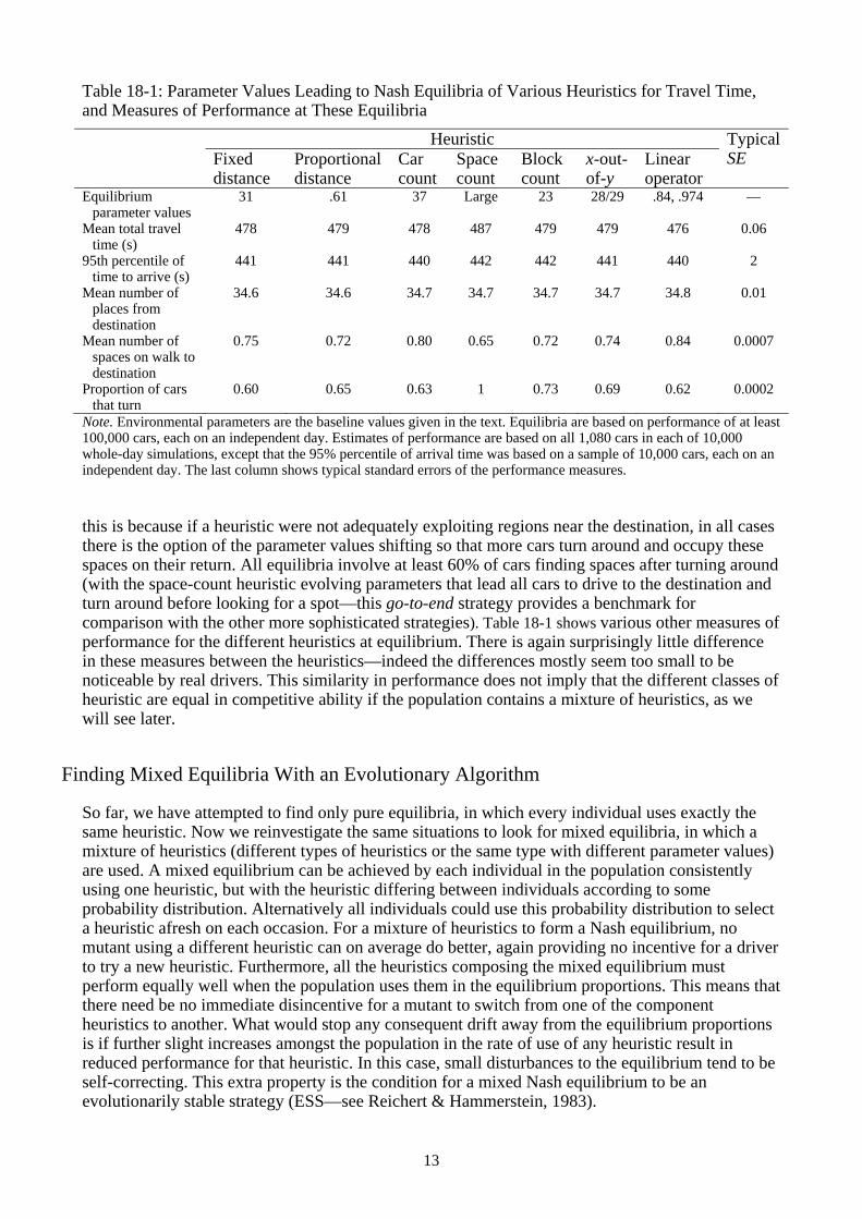
One obvious approach to comparing the ecological rationality of the heuristics is to let them compete directly: We describe such tournaments in the next section. But first, in this section, we allow each heuristic to compete just against versions of itself differing in parameter values, that is, in environments created when all drivers use the same parking heuristic. The heuristics will still be competing with themselves when we later allow them also to compete with other heuristics, so some of our understanding of these single-heuristic equilibria will carry over. Table 18-1 lists the parameter values that achieve pure Nash equilibria for each of the above heuristics, along with performance measures at equilibrium.

The proportional-distance heuristic at equilibrium takes spaces at least 61% of the way from the first parked car to the destination. The mean distance of the first parked car from the destination in our canonical setup is 74 parking places, so this heuristic will, on average, ignore vacancies farther than 29 places from the destination while driving toward it (which is about the same as the D = 31 of the fixed-distance heuristic at equilibrium).

The x-out-of-y heuristic at equilibrium has parameter values 28 out of 29. But the minimum of the performance surface is rather flat and the special cases where x = y perform almost as well when values of x are in the 20s. For the block-count heuristic (equivalent to restricting the x-out-of-y strategy set to x = y), the equilibrium value of x is 23. For the car-count heuristic (equivalent to the x-out-of-y strategy if y is very large), the equilibrium value of x is 37 parked cars to pass. The space-count heuristic only achieves an equilibrium when S is high enough that cars never park before turning around.

The equilibrium parameters of the linear-operator heuristic (a = .84, zpT = .974) are harder to interpret intuitively, but two examples illustrate its behavior. Starting from the first parked car encountered, it would not allow parking for at least 21 places after that, even if every place passed were full. Or if a space occurred just before the heuristic would have accepted it, then it would take a further solid block of 12 cars before another space would be acceptable. Thus, at their equilibria both the x-out-of-y and the linear-operator heuristics require a long stream of densely packed cars before parking is triggered. Nevertheless, they still sometimes accept parking places well before the fixed-distance, or even the proportional-distance, heuristics do at their equilibria.

The various heuristics at equilibrium produce distinct behaviors: Figure 18-3 shows some clear differences in whether a spot tends to be occupied before or after turning around. However, the different behaviors still produce environments that are remarkably similar, in terms of the distribution of occupied spaces averaged over the day (Figure 18-3, stepped curves). We think that

12

Figure 18-3: The distribution of parking positions at each of the equilibria in Table 18-1. Each black histogram (scale on the right) differentiates between cars parking before reaching the destination (to the left of the midline) and those parking after reaching it (to the right): Consequently the histogram also indicates the shape of the distribution of time to park. Each histogram is based on the parking positions from randomly selected single cars from 100,000 independent days. The stepped curve (scale on the left) shows the occupancy of each spot averaged over the entire day (on each of 10,000 independent days, we randomly sampled one moment within the range of times when cars could arrive). The panel at the bottom right superimposes these distributions of occupancy for all seven equilibria, showing how similar they are.

13

Table 18-1: Parameter Values Leading to Nash Equilibria of Various Heuristics for Travel Time, and Measures of Performance at These Equilibria

Heuristic Typical SE Fixed

distance Proportional distance

Car count

Space count

Block count

x-out-of-y

Linear operator

Equilibrium parameter values

31 .61 37 Large 23 28/29 .84, .974 —

Mean total travel time (s)

478 479 478 487 479 479 476 0.06

95th percentile of time to arrive (s)

441 441 440 442 442 441 440 2

Mean number of places from destination

34.6 34.6 34.7 34.7 34.7 34.7 34.8 0.01

Mean number of spaces on walk to destination

0.75 0.72 0.80 0.65 0.72 0.74 0.84 0.0007

Proportion of cars that turn

0.60 0.65 0.63 1 0.73 0.69 0.62 0.0002

Note. Environmental parameters are the baseline values given in the text. Equilibria are based on performance of at least 100,000 cars, each on an independent day. Estimates of performance are based on all 1,080 cars in each of 10,000 whole-day simulations, except that the 95% percentile of arrival time was based on a sample of 10,000 cars, each on an independent day. The last column shows typical standard errors of the performance measures. this is because if a heuristic were not adequately exploiting regions near the destination, in all cases there is the option of the parameter values shifting so that more cars turn around and occupy these spaces on their return. All equilibria involve at least 60% of cars finding spaces after turning around (with the space-count heuristic evolving parameters that lead all cars to drive to the destination and turn around before looking for a spot—this go-to-end strategy provides a benchmark for comparison with the other more sophisticated strategies). Table 18-1 shows various other measures of performance for the different heuristics at equilibrium. There is again surprisingly little difference in these measures between the heuristics—indeed the differences mostly seem too small to be noticeable by real drivers. This similarity in performance does not imply that the different classes of heuristic are equal in competitive ability if the population contains a mixture of heuristics, as we will see later.

Finding Mixed Equilibria With an Evolutionary Algorithm

So far, we have attempted to find only pure equilibria, in which every individual uses exactly the same heuristic. Now we reinvestigate the same situations to look for mixed equilibria, in which a mixture of heuristics (different types of heuristics or the same type with different parameter values) are used. A mixed equilibrium can be achieved by each individual in the population consistently using one heuristic, but with the heuristic differing between individuals according to some probability distribution. Alternatively all individuals could use this probability distribution to select a heuristic afresh on each occasion. For a mixture of heuristics to form a Nash equilibrium, no mutant using a different heuristic can on average do better, again providing no incentive for a driver to try a new heuristic. Furthermore, all the heuristics composing the mixed equilibrium must perform equally well when the population uses them in the equilibrium proportions. This means that there need be no immediate disincentive for a mutant to switch from one of the component heuristics to another. What would stop any consequent drift away from the equilibrium proportions is if further slight increases amongst the population in the rate of use of any heuristic result in reduced performance for that heuristic. In this case, small disturbances to the equilibrium tend to be self-correcting. This extra property is the condition for a mixed Nash equilibrium to be an evolutionarily stable strategy (ESS—see Reichert & Hammerstein, 1983).

14

The Evolutionary Algorithm

To search for mixed equilibria we used an evolutionary algorithm (Ruxton & Beauchamp, 2008). (Technically, ours is an evolutionary programming approach—see Bäck, Rudolph, & Schwefel, 1993.) The general operation of the evolutionary algorithm is to let a mixed population of strategies compete at parking, measure their mean performances, and then select a new population from the most successful, but adding some extra strategies modified from these winners. This process is repeated over many generations, leading to strategy change in the population in a manner akin to natural evolution.

Our evolutionary algorithm uses the same baseline parking environment as before, but now the 1,080 individuals parking on one day can each differ in the type of heuristic they use and the parameter values of their heuristic. Within each generation, the same 1,080 individuals compete over a large number (R) of independent days (i.e., each day the order of their arrival and their parking durations differ, but each individual uses the same strategy every day). The measure of the performance of an individual is the mean of its total travel times (parking search, walking, and driving away) over these R days.

Following this tournament, the best 10% of the individuals from the generation are selected and each of these is copied into the next generation with the same strategy and parameters. Each also replicates to form nine individuals with slightly mutated strategy parameters. The magnitude of mutation is randomly sampled from a normal distribution (or a discretized version in the case of integer parameters).8 In addition, there is a further round of more extensive mutations (hopeful monsters): Ten of the 1,080 individuals in the new generation are picked at random, their heuristic type is reallocated at random from those under consideration, and their parameter values are assigned anew from a uniform distribution over a plausible parameter range (e.g., for the fixed-distance heuristic, between 1 and 64). The performance of this new set of 1,080 individuals is then evaluated as before.

In the first generation, we start at R = 400 replicate days, which means that assessment of performance is inaccurate enough to allow some less good strategies to survive by chance initially (i.e., selection is weak). In this way we do not immediately shift the entire population onto heuristics that just happen to have good parameter values in the initial generations but give the less good heuristics (or regions of parameter space) a chance to improve. As the evolutionary algorithm proceeds, within a few generations there is typically some stability, but the distributions of parameter values of the survivors have rather broad peaks. This might be because there is disruptive selection favoring a diversity of parameter values, or it could be artifactual if the ratio of selection to mutation is insufficient for stabilizing selection to generate sharper peaks. The breadth of the peaks may in turn affect their mean value, because of the game-theoretic aspect of the parking situation. This may be realistic in that real drivers make mistakes both in their choices of good strategies and in enacting these strategies, and thus everyone’s strategies should be adapted to the likelihood of others also making such mistakes. However, to avoid the extra issue of deciding what level of driver error is realistic, in later generations we increase the selection versus mutation ratio as far as is practical, which typically reduces the breadth of the parameter distribution peaks.9

8. The standard deviation of this distribution depends on the absolute value of the parameter, so that mutation is less

in the case of a small integer or a proportion near 0 or 1 (for an integer parameter of value d, SD = 25+dV , or, in the

case of a proportion p, SD = 5/)1( ppV − , where V is a constant).

9. To do this, we typically double R every 10 generations, so that selection becomes more discriminating. The extent of mutation V is also decreased from 0.1 to 0.05 after 10 generations and to 0.035 after 20. Further reductions are not appropriate because otherwise integer parameter values mutate too rarely for evolution to occur in the time available for running the program. After 40 generations we also remove the hopeful-monster mutations.

15

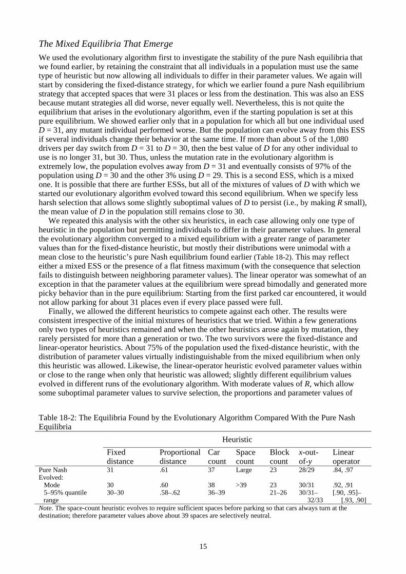
The Mixed Equilibria That Emerge

We used the evolutionary algorithm first to investigate the stability of the pure Nash equilibria that we found earlier, by retaining the constraint that all individuals in a population must use the same type of heuristic but now allowing all individuals to differ in their parameter values. We again will start by considering the fixed-distance strategy, for which we earlier found a pure Nash equilibrium strategy that accepted spaces that were 31 places or less from the destination. This was also an ESS because mutant strategies all did worse, never equally well. Nevertheless, this is not quite the equilibrium that arises in the evolutionary algorithm, even if the starting population is set at this pure equilibrium. We showed earlier only that in a population for which all but one individual used D = 31, any mutant individual performed worse. But the population can evolve away from this ESS if several individuals change their behavior at the same time. If more than about 5 of the 1,080 drivers per day switch from D = 31 to D = 30, then the best value of D for any other individual to use is no longer 31, but 30. Thus, unless the mutation rate in the evolutionary algorithm is extremely low, the population evolves away from D = 31 and eventually consists of 97% of the population using D = 30 and the other 3% using D = 29. This is a second ESS, which is a mixed one. It is possible that there are further ESSs, but all of the mixtures of values of D with which we started our evolutionary algorithm evolved toward this second equilibrium. When we specify less harsh selection that allows some slightly suboptimal values of D to persist (i.e., by making R small), the mean value of D in the population still remains close to 30.

We repeated this analysis with the other six heuristics, in each case allowing only one type of heuristic in the population but permitting individuals to differ in their parameter values. In general the evolutionary algorithm converged to a mixed equilibrium with a greater range of parameter values than for the fixed-distance heuristic, but mostly their distributions were unimodal with a mean close to the heuristic’s pure Nash equilibrium found earlier (Table 18-2). This may reflect either a mixed ESS or the presence of a flat fitness maximum (with the consequence that selection fails to distinguish between neighboring parameter values). The linear operator was somewhat of an exception in that the parameter values at the equilibrium were spread bimodally and generated more picky behavior than in the pure equilibrium: Starting from the first parked car encountered, it would not allow parking for about 31 places even if every place passed were full.

Finally, we allowed the different heuristics to compete against each other. The results were consistent irrespective of the initial mixtures of heuristics that we tried. Within a few generations only two types of heuristics remained and when the other heuristics arose again by mutation, they rarely persisted for more than a generation or two. The two survivors were the fixed-distance and linear-operator heuristics. About 75% of the population used the fixed-distance heuristic, with the distribution of parameter values virtually indistinguishable from the mixed equilibrium when only this heuristic was allowed. Likewise, the linear-operator heuristic evolved parameter values within or close to the range when only that heuristic was allowed; slightly different equilibrium values evolved in different runs of the evolutionary algorithm. With moderate values of R, which allow some suboptimal parameter values to survive selection, the proportions and parameter values of

Table 18-2: The Equilibria Found by the Evolutionary Algorithm Compared With the Pure Nash Equilibria

Heuristic

Fixed distance

Proportional distance

Car count

Space count

Block count

x-out-of-y

Linear operator

Pure Nash 31 .61 37 Large 23 28/29 .84, .97Evolved: Mode 5–95% quantile

range

30 30–30

.60 .58–.62

38 36–39

>39 23 21–26

30/31 30/31– 32/33

.92, .91 [.90, .95]– [.93, .90]

Note. The space-count heuristic evolves to require sufficient spaces before parking so that cars always turn at the destination; therefore parameter values above about 39 spaces are selectively neutral.

16

these two heuristics remain stable indefinitely. But with higher selection pressure from large values of R, the proportions start to oscillate and then diverge, which can eventually drive the linear-operator heuristic to extinction. However, this extinction would only be temporary whenever mutants are introduced, because each of these heuristics can invade a population composed entirely of the other heuristic. Furthermore, such harsh selection pressure is unrepresentative of the real world, so an equilibrium with both heuristics persisting is more relevant.

It remains possible that some particular combinations of the other heuristics are also ESSs, since the evolutionary algorithm does not systematically check all combinations of parameter values. But because all starting conditions that we investigated converged to the identified two-heuristic equilibrium, we claim that it is the most likely ESS to arise among these strategies in this environment. What we cannot yet say is whether this mixture of two heuristics is stable against invasion by heuristics that we have not considered. Given that the ESS consists of some individuals that respond to local density and some that use a fixed distance from the destination (and/or individuals that sometimes do each), a plausible candidate for a heuristic that would outcompete these would be one that combined these two approaches. Moreover, it seems intuitively reasonable that drivers might somehow combine such obviously relevant cues as position and density, rather than using only one piece of information. We investigate such a heuristic at the end of the next section.

Explaining Heuristic Competitiveness via Environment Structure

To understand why some types of heuristics outcompete others in the search for good parking spaces, it is necessary to consider the structure of the environment in which they operate—this is the central tenet of ecological rationality. As we have emphasized, the environment structure for this parking task is created by the heuristics that the population is using. Figure 18-3 demonstrates that some broad structural features of the patterns of occupancy are fairly consistent across environments, at least among those produced by well-adapted heuristics (i.e., with near-equilibrium parameter values). Here we focus on another consistent environmental feature and its implications for strategy performance.

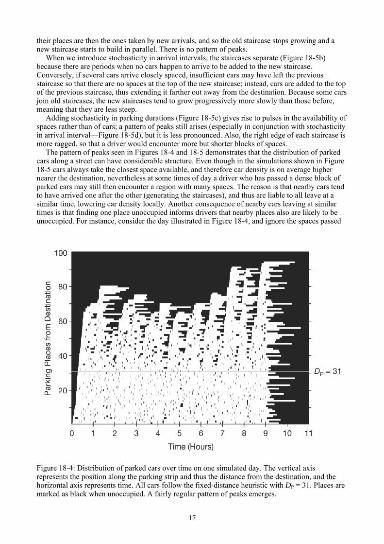
The feature can be seen in Figure 18-4, which shows the results of a simulation in which all drivers decide whether to accept each parking space using the fixed-distance heuristic with the pure ESS aspiration level D = 31. The vertical axis represents the position along the parking strip, with the destination at the bottom; the distribution of cars in the parking strip is plotted against time on the horizontal axis. Thus one “column” in the figure corresponds to the presence or absence of parked cars at all distances from the destination at one particular time step. Clear structure is apparent: The distribution of parked cars over time is characterized by a striking pattern of peaks occurring fairly regularly in time, although varying in height. This is typical also of our simulations of the other parking heuristics. We did not expect such a pattern and we are not aware of others having reported it either in computer simulations or in the field. Its consequence is that drivers arriving at different times can encounter the first (farthest from destination) parked car at very different positions, after which large blocks of spaces may appear.

A likely prerequisite for this pattern to occur is that spaces are not chosen randomly; rather, parking spaces closer to the destination must have a higher probability of being chosen. This is normally the case with well-adapted heuristics, since they are sufficiently ambitious that quite often cars have to turn around at the destination and then will take the closest available space on their return. To demonstrate how this behavior leads to the observed structure, we ran simplified simulations in which each car instantaneously occupied the space closest to the destination. First, we kept the parking duration and the interval between the arrival of cars constant, which resulted in an overlapping-staircase-like pattern of occupancy over time (Figure 18-5a). The first staircase arises because later arrivals have to take parking places progressively farther from the destination. Then, because the order in which cars depart follows the same sequence as their arrival, it is cars closest to the destination (i.e., those that formed the base of the staircase) that start leaving first;

17

their places are then the ones taken by new arrivals, and so the old staircase stops growing and a new staircase starts to build in parallel. There is no pattern of peaks.

When we introduce stochasticity in arrival intervals, the staircases separate (Figure 18-5b) because there are periods when no cars happen to arrive to be added to the new staircase. Conversely, if several cars arrive closely spaced, insufficient cars may have left the previous staircase so that there are no spaces at the top of the new staircase; instead, cars are added to the top of the previous staircase, thus extending it farther out away from the destination. Because some cars join old staircases, the new staircases tend to grow progressively more slowly than those before, meaning that they are less steep.

Adding stochasticity in parking durations (Figure 18-5c) gives rise to pulses in the availability of spaces rather than of cars; a pattern of peaks still arises (especially in conjunction with stochasticity in arrival interval—Figure 18-5d), but it is less pronounced. Also, the right edge of each staircase is more ragged, so that a driver would encounter more but shorter blocks of spaces.

The pattern of peaks seen in Figures 18-4 and 18-5 demonstrates that the distribution of parked cars along a street can have considerable structure. Even though in the simulations shown in Figure 18-5 cars always take the closest space available, and therefore car density is on average higher nearer the destination, nevertheless at some times of day a driver who has passed a dense block of parked cars may still then encounter a region with many spaces. The reason is that nearby cars tend to have arrived one after the other (generating the staircases), and thus are liable to all leave at a similar time, lowering car density locally. Another consequence of nearby cars leaving at similar times is that finding one place unoccupied informs drivers that nearby places also are likely to be unoccupied. For instance, consider the day illustrated in Figure 18-4, and ignore the spaces passed

Figure 18-4: Distribution of parked cars over time on one simulated day. The vertical axis represents the position along the parking strip and thus the distance from the destination, and the horizontal axis represents time. All cars follow the fixed-distance heuristic with DP = 31. Places are marked as black when unoccupied. A fairly regular pattern of peaks emerges.

18

Figure 18-5: Distribution of parked cars over time (plotted as in Figure 18-4) under different conditions: (a) Interval between arriving cars and parking duration held constant, creating overlapping staircases of occupied parking places. (b) Stochasticity added to arrival times, causing staircases to separate. (c) Stochasticity added to parking durations, generating uneven peaks. (d) Stochasticity in both arrival times and parking durations (as in Figure 18-4).

19

prior to encountering the first parked car; even though overall only one in six parking places is unoccupied, a space is more likely to be immediately followed by another space than by a parked car. The existence of this autocorrelation invalidates the assumptions of previous analytic models (e.g., MacQueen & Miller, 1960; Tamaki, 1988) that the probability of a parking place being occupied is independent of the occupancy of other places. We will now illustrate ways that the structure in Figures 18-4 and 18-5 can help us understand why (and when) some heuristics function better than others.

First, we can see why the space-count heuristic was outcompeted by the policy of only parking after passing the destination. The autocorrelation in the occurrence of spaces means that encountering more spaces than usual is a reason to expect further spaces to occur ahead, so search should continue; instead, the space-count heuristic is triggered to accept a space.

The proportional-distance heuristic might a priori seem a good means to spot times of day when there are gaps between the staircases in Figure 18-4, and to search nearer the destination at such times. But in fact it is poor at this job because there can be one car near the top of a staircase that remains parked for much longer than the mean (the gamma distribution of parking durations is right skewed) so that the heuristic becomes blind to any low density beyond. Another problem is that when spaces are appearing near the destination the current staircase stops growing, but cars just arrived near the top of the staircase remain for some time; when they disappear the desirable spaces near the destination have long been occupied. So the proportional-distance heuristic’s emphasis on the very first car encountered may be misguided. The space-count and car-count heuristics may similarly be poorly designed in their partial dependence on occupancy far from the destination as a means to predict occupancy near the destination.

The linear-operator, x-out-of-y, and block-count heuristics all respond to local density and thus can utilize the local positive autocorrelation in vacancies. When they detect a high density of spaces they do not park, gambling on there being more spaces ahead. We analyzed how the linear-operator heuristic performs in the mixed ESS with the fixed-distance heuristic. The linear-operator heuristic is adaptive in that at times when the peaks are growing because some cars are encountering no spaces, it accepts spaces before the fixed-distance heuristic would (and therefore has to turn around less often), whereas at times of lower density when many parked cars are leaving, it tends to be more ambitious than the fixed-distance heuristic. We are not sure why the linear operator is the most successful of the density-dependent heuristics, but it may be important that it both avoids being triggered until well after the first car is encountered and yet is not overly influenced by the occasional gap in an otherwise high-density sequence. Potentially these density-dependent heuristics have to be very picky to avoid being triggered in areas of high density a long way from the destination, but this is too picky once they get close. Thus, a superior heuristic might wait until within a certain distance of the destination to invoke a less picky density-dependent trigger.

Accordingly, we tested such a distance-and-density heuristic. This requires the conditions for both the fixed-distance and the block-count heuristics to be simultaneously satisfied. We chose the block-count heuristic to monitor density because it requires only one parameter. The distance-and-density heuristic indeed invades the mixed fixed-distance and linear-operator ESS, driving both to extinction. It is also the only surviving strategy when pitted against all seven previous heuristics. At equilibrium the parameters of the distance-and-density heuristic are somewhat broadly spread: The parameter value of the fixed-distance component averages 36, but values from 32 to 41 may also persist; the parameter value of the block-count component averages 12, but values from 9 to 17 may also persist. Larger values of one parameter are associated with larger values of the other, so successful versions that are less picky about how far away to accept a space are more picky about how long the block of cars must be to trigger acceptance. There is no pure Nash equilibrium.

Conclusions: The Game of Parking

A common starting point for people thinking about how they search for a parking space, and for researchers developing models to try to understand the process of searching for parking, is to suppose that drivers proceed some way toward their destination until they are “close enough” and

20

then take the next available space. And indeed this fixed-distance heuristic is optimal in an idealized world where parking spaces are distributed independently. But in the real world, as people park in spaces and exit them later, they create structure in the environment of available spaces that other drivers are searching through. We investigated the consequences in a simple model system and demonstrated how the aspiration level of the fixed-distance heuristic should adjust to an environment created by other drivers using the same heuristic. In theory there was a stable equilibrium in which everybody using one particular aspiration level would create an environment where no other aspiration level could do better. However, everybody in real life using similar aspiration levels seems unlikely, especially given our demonstrations that very different parameter values are to be expected among drivers if they are influenced by their experiences of parking in different underlying environments (e.g., with different arrival rates of competing parkers, or different street layouts) or if they differ in which performance criteria most matter to them.

Nevertheless, our idealized model system proved illuminating when assessing other plausible sorts of simple parking heuristics. All could give rise to pure equilibria yielding a similar mean performance and distribution of parked cars; but when we allowed different heuristics to compete, a mixture of the fixed-distance and linear-operator heuristics consistently prevailed. A more detailed examination of the environments created by these heuristics helped to explain why. In particular, there was considerable clumping in the distribution of parking spaces, but where these clumps occurred moved during the day, which the linear-operator heuristic could exploit. This led us to design a superior two-criterion heuristic that allowed parking only if both the destination was sufficiently close and there had been a lack of vacancies in the last few places passed. Because the autocorrelation in the occurrence of spaces is likely to be a common phenomenon in many different parking situations and should occur regardless of the performance criterion, it may be a widely applicable conclusion that such distance-and-density heuristics are a good choice. We used the simplest block-count component mechanism to assess the local density of vacancies, so somewhat more complex heuristics (nevertheless well within our cognitive abilities) could well be even more competitive. However, there remains the problem that the appropriate parameter values of such heuristics may be difficult for drivers to select; as with the fixed-distance heuristic, these are likely to depend considerably on underlying aspects of the environment such as arrival rates and street topology.

We have emphasized the need to consider dynamic and game-theoretic, strategic interactions in our analysis of what are good parking strategies. But do drivers really take these aspects into account when looking for parking spaces? Of course, based on their experience with what has worked previously, drivers could be blindly applying rules adapted to the game-theoretic situation without thinking about why they work. Alternatively, although drivers are clearly not carrying out in their heads the kind of computationally intensive analysis presented in this chapter, they may be applying rules that their intuition suggests are adaptive in a competitive game-theoretic context. This intuition might be as simple as a justified expectation that there is some autocorrelation in the occurrence of parking spaces, or instead our ever-active brains might be using much more complex calculations even though our underlying theories may be misguided. Where we get our parking heuristics from is a hard problem to solve, but empirical investigations can at least start by determining which heuristics people actually apply in particular parking contexts, and how these may fit to the perceived structure of the environment.

References

Anderson, S. P., & de Palma, A. (2004). The economics of pricing parking. Journal of Urban Economics, 55, 1–20.

Arnott, R., & Rowse, J. (1999). Modeling parking. Journal of Urban Economics, 45, 97–124. Bäck, T., Rudolph, G., & Schwefel, H.-P. (1993). Evolutionary programming and evolution

strategies: Similarities and differences. In D. B. Fogel & W. Atmars (Eds.), Proceedings of the Second Annual Conference on Evolutionary Programming (pp. 11–22). San Diego, CA: Evolutionary Programming Society.

21

Bearden, J. N., & Connolly, T. (2007). Multi-attribute sequential search. Organizational Behavior and Human Decision Processes, 103, 147–158.

Corbin, R. M., Olson, C. L., & Abbondanza, M. (1975). Context effects in optional stopping decisions. Organizational Behavior and Human Performance, 14, 207–216.

DeGroot, M. H. (1970). Optimal statistical decisions. New York: McGraw–Hill. Dudey, T., & Todd, P.M. (2002). Making good decisions with minimal information: Simultaneous

and sequential choice. Journal of Bioeconomics, 3, 195–215. Ferguson, T. S. (n.d.). Optimal stopping and applications. Retrieved from

http://www.math.ucla.edu/~tom/Stopping/Contents.html Fudenberg, D., & Tirole, J. (1991). Game theory. Cambridge, MA: MIT Press. Groß, R., Houston, A. I., Collins, E. J., McNamara, J. M., Dechaume-Moncharmont, F.-X., &

Franks, N. R. (2008). Simple learning rules to cope with changing environments. Journal of the Royal Society Interface, 5, 1193–1202.

Hey, J. D. (1982). Search for rules for search. Journal of Economic Behavior and Organization, 3, 65–81.

Hutchinson, J. M. C., & Halupka, K. (2004). Mate choice when males are in patches: Optimal strategies and good rules of thumb. Journal of Theoretical Biology, 231, 129–151.

Hutchinson, J. M. C., McNamara, J. M., & Cuthill, I. C. (1993). Song, sexual selection, starvation and strategic handicaps. Animal Behaviour, 45, 1153–1177.

Kreps, D. M. (1990). Game theory and economic modelling. Oxford: Clarendon Press. Lee, M. D. (2006). A hierarchical Bayesian model of human decision-making on an optimal

stopping problem. Cognitive Science, 30, 555–580. MacQueen, J., & Miller, R. G., Jr. (1960). Optimal persistence policies. Operations Research, 8,

362–380. Martin, A., & Moon, P. (1992). Purchasing decisions, partial knowledge, and economic search:

Experimental and simulation evidence. Journal of Behavioral Decision Making, 5, 253–266. Reichert, S. E., & Hammerstein, P. (1983). Game theory in the ecological context. Annual Reviews

of Ecology and Systematics, 14, 377–409. Roitberg, B. D., Reid, M. L., & Li, C. (1993). Choosing hosts and mates: The value of learning. In

D. R. Papaj & A. C. Lewis (Eds.), Insect learning: ecological and evolutionary perspectives (pp 174–194). New York: Chapman & Hall.

Ruxton, G. D., & Beauchamp, G. (2008). The application of genetic algorithms in behavioural ecology, illustrated with a model of anti-predator vigilance. Journal of Theoretical Biology, 250, 435–448.

Salomon, I. (1986). Towards a behavioural approach to city centre parking : The case of Jerusalem's CBD. Cities, 3, 200–208.

Seale, D. A., & Rapoport, A. (1997). Sequential decision making with relative ranks: An experimental investigation of the ‘secretary problem.’ Organizational Behavior and Human Decision Processes, 69, 221–236.

Seale, D. A., & Rapoport, A. (2000). Optimal stopping behavior with relative ranks: The secretary problem with unknown population size. Journal of Behavioral Decision Making, 13, 391–411.

Simon, H. A. (1955). A behavioral model of rational choice. Quarterly Journal of Economics, 69, 99–118.

Tamaki, M. (1985). Adaptive approach to some stopping problems. Journal of Applied Probability, 22, 644–652.

Tamaki, M. (1988). Optimal stopping in the parking problem with U-turn. Journal of Applied Probability, 25, 363–374.

Thompson, R. G., & Richardson, A. J. (1998). A parking search model. Transportation Research Part A: Policy and Practice, 32, 159–170.

Todd, P. M., & Miller, G. F. (1999). From pride and prejudice to persuasion: Satisficing in mate search. In G. Gigerenzer, P. M. Todd, & the ABC Research Group, Simple heuristics that make us smart (pp. 287–308). New York: Oxford University Press.

Vanderbilt, T. (2008). Traffic: Why we drive the way we do (and what it says about us). New York: Knopf.

22

Van Der Goot, D. (1982). A model to describe the choice of parking places. Transportation Research Part A: General, 16, 109–115.

Wiegmann, D. D. & Morris, M. R. (2005). Search behavior and mate choice. Recent Research Developments in Experimental & Theoretical Biology, 1, 201-216.

Young, W. (1986). A model of vehicles movements in parking facilities. Mathematics and Computers in Simulation, 28, 305–309.