Slide 1

18-660: Numerical Methods for Engineering Design and Optimization

Xin Li Department of ECE

Carnegie Mellon University Pittsburgh, PA 15213

Slide 2

Overview

Introduction Numerical computation Examples and applications

Slide 3

Numerical Computation

Numerical computation: approximation techniques and algorithms to numerically solve mathematical problems Not all mathematical problems have closed-form solutions

Mathematical examples

Solve nonlinear algebraic equations Find minimum of a nonlinear function Determine eigenvalues of a matrix

This course will encompass various aspects of numerical

methods and their applications Linear & nonlinear solver, nonlinear optimization, randomized

algorithm, etc.

Slide 4

Numerical Computation

Numerical computation is an important tool to solve many practical engineering problems

PageRank finds the eigenvector of a 1010-by-1010 matrix – the largest matrix computation in the world

Airlines use optimization algorithms to decide ticket prices, airplane assignments and fuel needs

Slide 5

Numerical Computation

Several additional real-world examples:

Car companies run computer simulations of car crashes to identify safety issues

Wall street runs statistical simulation tools to predict stock prices

Slide 6

Brief History of Numerical Computation

Before 1950s

Algorithms Linear interpolation Newton’s method Gaussian elimination

Tools

Hand calculation Formula handbook Data table

Carl Friedrich Gauss (1777-1855) German Mathematician

Slide 7

Brief History of Numerical Computation

After 1950s The invention of modern computers motivates the development

of a great number of new numerical algorithms

1E+04

1E+05

1E+06

1E+07

1E+08

1E+09

1E+10

1E+1119

71

1974

1979

1984

1986

1990

1994

1996

1999

2000

2002

2005

2005

2006

2006

2007

2008

Inst

ruct

ion

Per

Sec

ond

1E+05

1E+06

1E+07

1E+08

1E+09

1E+10

CP

U F

requ

ency

(Hz)

IPS Freq

Slide 8

Numerical Computation Problems

Ordinary and partial differential equations

Regression

Classification

Slide 9

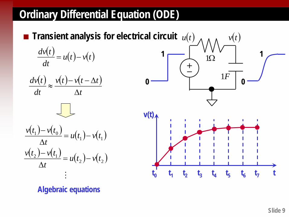
Ordinary Differential Equation (ODE)

Transient analysis for electrical circuit

F1

Ω11

0

1

0

( ) ( ) ( )tvtudt

tdv−=

( )tu ( )tv

( ) ( ) ( )t

ttvtvdt

tdv∆

∆−−≈

t

v(t)

t1 t0 t2 t3 t4 t5 t6 t7

( ) ( ) ( ) ( )

( ) ( ) ( ) ( )

2212

1101

tvtut

tvtv

tvtut

tvtv

−=∆−

−=∆−

Algebraic equations

Slide 10

Partial Differential Equation (PDE)

Thermal analysis: heat conduction is governed by partial differential equation (PDE):

( ) ( )[ ] ( )tzyxptzyxTt

tzyxTCp ,,,,,,,,,+∇⋅⋅∇=

∂

∂⋅⋅ κρ

Material density (kg/m3)

Specific heat capacity (Joules/K-kg)

Thermal conductivity (Watts/K-m)

Power density of heat sources

(Watts/m3)

Slide 11

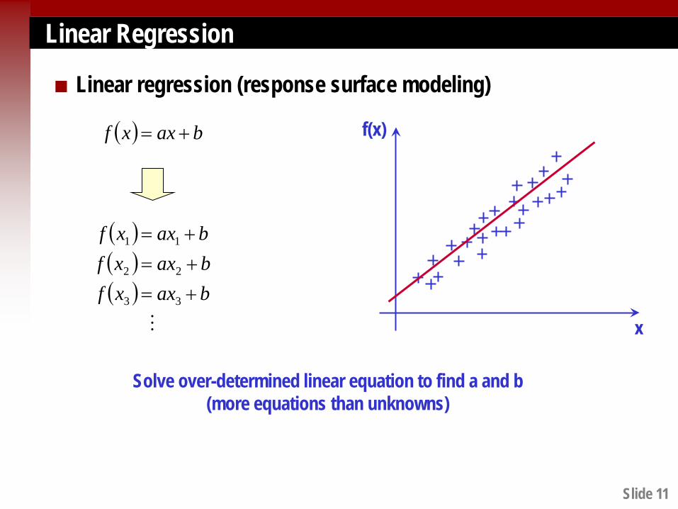
Linear Regression

Linear regression (response surface modeling)

f(x)

x

( ) baxxf +=

( )( )( )

baxxfbaxxfbaxxf

+=+=+=

33

22

11

Solve over-determined linear equation to find a and b (more equations than unknowns)

Slide 12

Linear Regression

Linear regression with regularization

Original image Recovered image

BA =α 1

2

2min αλαα

⋅+− BA

Least-squares error

L1-norm regularization

Slide 13

Classification

Support vector machine (SVM)

Feature x1

Feat

ure x

2

Margin

( ) ( )( )

<≥

+=BClassAClass

CXWXf T

0 0

SVM Coefficients Features

( )( )BClassXCXW

AClassXCXWW

T

T

0 0S.T.

min 2

2

∈<+∈≥+

L2-norm (maximize margin)

Solve convex quadratic programming to find W and C

Slide 14

Classification

Brain computer interface based on classification

Neural signal recording

Neural signal processing

Movement decoding

Feedback

Methods: filtering; signal subspace methods … Tool Boxes: MNE-Suite; FieldTrip; MaxFilter …

-0.5 0 0.5 1 1.5 2-2.5

-2

-1.5

-1

-0.5

0

0.5

1

1.5

2

Time (Sec.)

Ampl

itude

(Nor

mal

ized)

-0.5 0 0.5 1 1.5 2-2.5

-2

-1.5

-1

-0.5

0

0.5

1

1.5

2

Time (Sec.)

Ampl

itude

(Nor

mal

ized)

MEG EEG

Slide 15

Summary

Numerical computation Examples and applications