1714 IEEE TRANSACTIONS ON INFORMATION THEORY, VOL. 57, …tensorlab.cms.caltech.edu/users/anima/pubs/TATW_IT09.pdf · 1714 IEEE TRANSACTIONS ON INFORMATION THEORY, VOL. 57, NO. 3,

1714 IEEE TRANSACTIONS ON INFORMATION THEORY, VOL. 57, NO. 3, MARCH 2011

A Large-Deviation Analysis of theMaximum-Likelihood Learning of

Markov Tree StructuresVincent Y. F. Tan, Member, IEEE, Animashree Anandkumar, Member, IEEE, Lang Tong, Fellow, IEEE, and

Alan S. Willsky, Fellow, IEEE

Abstract—The problem of maximum-likelihood (ML) estima-tion of discrete tree-structured distributions is considered. Chowand Liu established that ML-estimation reduces to the construc-tion of a maximum-weight spanning tree using the empiricalmutual information quantities as the edge weights. Using thetheory of large-deviations, we analyze the exponent associatedwith the error probability of the event that the ML-estimate ofthe Markov tree structure differs from the true tree structure,given a set of independently drawn samples. By exploiting thefact that the output of ML-estimation is a tree, we establish thatthe error exponent is equal to the exponential rate of decay of asingle dominant crossover event. We prove that in this dominantcrossover event, a non-neighbor node pair replaces a true edgeof the distribution that is along the path of edges in the true treegraph connecting the nodes in the non-neighbor pair. Using ideasfrom Euclidean information theory, we then analyze the scenarioof ML-estimation in the very noisy learning regime and showthat the error exponent can be approximated as a ratio, whichis interpreted as the signal-to-noise ratio (SNR) for learning treedistributions. We show via numerical experiments that in thisregime, our SNR approximation is accurate.

Index Terms—Error exponent, Euclidean information theory,large-deviations principle, Markov structure, maximum-likeli-hood (ML) distribution estimation, tree-structured distributions.

I. INTRODUCTION

T HE estimation of a distribution from samples is a classicaland an important generic problem in machine learning and

statistics and is challenging for high-dimensional multivariate

Manuscript received May 06, 2009; revised October 19, 2010; acceptedNovember 18, 2010. Date of current version February 18, 2011. This workwas supported in part by A*STAR, Singapore, by a MURI funded throughARO Grant W911NF-06-1-0076 and by AFOSR Grant FA9550-08-1-0180and in part by the Army Research Office MURI Program under awardW911NF-08-1-0238. The material in this paper was presented in part at theInternational Symposium on Information Theory (ISIT), Seoul, Korea, June2009. V. Y. F. Tan performed this work while at MIT.

V. Y. F. Tan is with the Department of Electrical and Computer Engineering,University of Wisconsin-Madison, WI 53706 USA (e-mail: [email protected]).

A. Anandkumar is with the Center for Pervasive Communications and Com-puting, Electrical Engineering and Computer Science Department, Universityof California, Irvine 92697 USA (e-mail: [email protected]).

L. Tong is with the School of Electrical and Computer Engineering, CornellUniversity, Ithaca, NY 14853 USA (e-mail: [email protected]).

A. S. Willsky is with the Stochastic Systems Group, Laboratory for Informa-tion and Decision Systems, Massachusetts Institute of Technology, Cambridge,MA 02139 USA (e-mail: [email protected]).

Communicated by A. Krzyzak, Associate Editor for Pattern Recognition, Sta-tistical Learning, and Inference.

Color versions of one or more of the figures in this paper are available onlineat http://ieeexplore.ieee.org.

Digital Object Identifier 10.1109/TIT.2011.2104513

distributions. In this respect, graphical models [2] provide a sig-nificant simplification of joint distribution as the distribution canbe factorized according to a graph defined on the set of nodes.Many specialized algorithms [3]–[9] exist for exact and approx-imate learning of graphical models Markov on sparse graphs.

There are many applications of learning graphical models,including clustering and dimensionality reduction. Suppose wehave genetic variables and we would like to group the onesthat are similar together. Then the construction of a graphicalmodel provides a visualization of the relationship betweengenes. Those genes that have high degree are highly correlatedto many other genes (e.g., those in its neighborhood). Thelearning of a graphical model may also provide the means tojudiciously remove redundant genes from the model, thus re-ducing the dimensionality of the data, leading to more efficientinference of the effects of the genes subsequently.

When the underlying graph is a tree, the Chow-Liu algorithm[3] provides an efficient method for the maximum-likelihood(ML) estimation of the probability distribution from a set ofi.i.d. samples drawn from the distribution. By exploiting theMarkov tree structure, this algorithm reduces the ML-estimationproblem to solving a maximum-weight spanning tree (MWST)problem. In this case, it is known that the ML-estimator learnsthe distribution correctly asymptotically, and hence, is consis-tent [10].

While consistency is an important qualitative property forany estimator, the study of the rate of convergence, a precisequantitative property, is also of great practical interest. Weare interested in the rate of convergence of the ML-estimator(Chow-Liu algorithm) for tree distributions as we increase thenumber of samples. Specifically, we study the rate of decay ofthe error probability or the error exponent of the ML-estimatorin learning the tree structure of the unknown distribution. Alarger exponent means that the error probability in structurelearning decays more rapidly. In other words, we need rela-tively few samples to ensure that the error probability is belowsome fixed level . Such model are thus “easier” to learn.We address the following questions: Is there exponential decayof the probability of error in structure learning as the numberof samples tends to infinity? If so, what is the exact errorexponent, and how does it depend on the parameters of thedistribution? Which edges of the true tree are most-likely to bein error; in other words, what is the nature of the most-likelyerror in the ML-estimator? We provide concrete and intuitiveanswers to the above questions, thereby providing insightsinto how the parameters of the distribution influence the error

0018-9448/$26.00 © 2011 IEEE

TAN et al.: A LARGE-DEVIATION ANALYSIS OF THE MAXIMUM-LIKELIHOOD LEARNING OF MARKOV TREE STRUCTURES 1715

exponent associated with learning the structure of discrete treedistributions.

A. Main Contributions

There are three main contributions in this paper. First, usingthe large-deviation principle (LDP) [11] we prove that the most-likely error in ML-estimation is a tree which differs from the truetree by a single edge. Second, again using the LDP, we derive theexact error exponent for ML-estimation of tree structures. Third,we provide a succinct and intuitive closed-form approximationfor the error exponent which is tight in the very noisy learningregime, where the individual samples are not too informativeabout the tree structure. The approximate error exponent has avery intuitive explanation as the signal-to-noise ratio (SNR) forlearning.

We analyze the error exponent (also called the inaccuracyrate) for the estimation of the structure of the unknown tree dis-tribution. For the error event that the structure of the ML-esti-mator given samples differs from the true tree structure

of the unknown distribution , the error exponent is givenby

(1)

To the best of our knowledge, error-exponent analysis fortree-structure learning has not been considered before (SeeSection I-B for a brief survey of the existing literature onlearning graphical models from data).

Finding the error exponent in (1) is not straightforwardsince in general, one has to find the dominant error event withthe slowest rate of decay among all possible error events [11, Ch.1]. For learning the structure of trees, there are a total ofpossible error events,1 where is the dimension (number of vari-ables or nodes) of the unknown tree distribution . Thus, inprinciple, one has to consider the information projection [13] of

on all these error trees. This rules out brute-force informationprojection approaches for finding the error exponent in (1), es-pecially for high-dimensional data.

In contrast, we establish that the search for the dominant errorevent for learning the structure of the tree can be limited to apolynomial-time search space (in ). Furthermore, we establishthat this dominant error event of the ML-estimator is given bya tree which differs from the true tree by only a single edge.We provide a polynomial algorithm with com-plexity to find the error exponent in (1), where is thediameter of the tree . We heavily exploit the mechanism ofthe ML Chow-Liu algorithm [3] for tree learning to establishthese results, and specifically, the fact that the ML-estimator treedistribution depends only on the relative order of the empiricalmutual information quantities between all the node pairs (andnot their absolute values).

Although we provide a computationally-efficient way to com-pute the error exponent in (1), it is not available in closed-form.In Section VI, we use Euclidean information theory [14], [15] toobtain an approximate error exponent in closed-form, which can

1Since the ML output � and the true structure � are both spanning treesover � nodes and since there are � possible spanning trees [12], we have� � � number of possible error events.

be interpreted as the signal-to-noise ratio (SNR) for tree struc-ture learning. Numerical simulations on various discrete graph-ical models verify that the approximation is tight in the verynoisy regime.

In Section VII, we extend our results to the case when the truedistribution is not a tree. In this case, given samples drawnindependently from , we intend to learn the optimal reverseinformation projection onto the set of trees. Importantly, if

is not a tree, there may be several trees that are optimal pro-jections [10] and this requires careful consideration of the errorevents. We derive the error exponent even in this scenario.

B. Related Work

The seminal work by Chow and Liu in [3] focused on learningtree models from data samples. The authors showed that thelearning of the optimal tree distribution essentially decouplesinto two distinct steps: (i) a structure learning step and (ii) a pa-rameter learning step. The structure learning step, which is thefocus on this paper, can be performed efficiently using a max-weight spanning tree algorithm with the empirical mutual infor-mation quantities as the edge weights. The parameter learningstep is a maximum-likelihood estimation procedure where theparameters of the learned model are equal to those of the empir-ical distribution. Chow and Wagner [10], in a follow-up paper,studied the consistency properties of the Chow-Liu algorithmfor learning trees. They concluded that if the true distribution isMarkov on a unique tree structure, then the Chow-Liu learningalgorithm is asymptotically consistent. This implies that as thenumber of samples tends to infinity, the probability that thelearned structure differs from the (unique) true structure tendsto zero.

Unfortunately, it is known that the exact learning of generalgraphical models is NP-hard [16], but there have been severalworks to learn approximate models. For example, Chechetkaand Guestrin [4] developed good approximations for learningthin junction trees [17] (junction trees where the sizes of themaximal cliques are small). Heckerman [18] proposed learningthe structure of Bayesian networks by using the Bayesian Infor-mation Criterion [19] (BIC) to penalize more complex modelsand by putting priors on various structures. Other authors usedthe maximum entropy principle or (sparsity-enforcing) regu-larization as approximate graphical model learning techniques.In particular, Dudik et al. [9] and Lee et al. [6] provide strongconsistency guarantees on the learned distribution in terms ofthe log-likelihood of the samples. Johnson et al. [7] also useda similar technique known as maximum entropy relaxation(MER) to learn discrete and Gaussian graphical models. Wain-wright et al. [5] proposed a regularization method for learningthe graph structure based on logistic regression and providedstrong theoretical guarantees for learning the correct structureas the number of samples, the number of variables, and theneighborhood size grow. In a similar work, Meinshausen andBuehlmann [8] considered learning the structure of arbitraryGaussian models using the Lasso [20]. They show that theerror probability of learning the wrong structure, under somemild technical conditions on the neighborhood size, decaysexponentially even when the size of the graph grows withthe number of samples . However, the rate of decay is not


provided explicitly. Zuk et al. [21] provided bounds on thelimit inferior and limit superior of the error rate for learningthe structure of Bayesian networks but, in contrast to our work,these bounds are not asymptotically tight. In addition, the workin Zuk et al. [21] is intimately tied to the BIC [19], whereas ouranalysis is for the Chow-Liu ML tree learning algorithm [3]. Amodification of the Chow-Liu learning algorithm has also beenapplied to learning the structure of latent trees where only asubset of variables are observed [22].

There have also been a series of papers [23]–[26] that quantifythe deviation of the empirical information-theoretic quantitiesfrom their true values by employing techniques from large-de-viations theory. Some ideas from these papers will turn out tobe important in the subsequent development because we exploitconditions under which the empirical mutual information quan-tities do not differ “too much” from their nominal values. Thiswill ensure that structure learning succeeds with high proba-bility.

C. Paper Outline

This paper is organized as follows: In Sections II and III, westate the system model and the problem statement and providethe necessary preliminaries on undirected graphical models andthe Chow-Liu algorithm [3] for learning tree distributions. InSection IV, we derive an analytical expression for the crossoverrate of two node pairs. We then relate the crossover rates to theoverall error exponent in Section V. We also discuss some con-nections of the problem we solve here with robust hypothesistesting. In Section VI, we leverage on ideas in Euclidean infor-mation theory to state sufficient conditions that allow approxi-mations of the crossover rate and the error exponent. We obtainan intuitively appealing closed-form expression. By redefiningthe error event, we extend our results to the case when the truedistribution is not a tree in Section VII. We compare the trueand approximate crossover rates by performing numerical ex-periments for a given graphical model in Section VIII. Perspec-tives and possible extensions are discussed in Section IX.

II. SYSTEM MODEL AND PROBLEM STATEMENT

A. Graphical Models

An undirected graphical model [2] is a probability distribu-tion that factorizes according to the structure of an underlyingundirected graph. More explicitly, a vector of random variables

is said to be Markov on a graphwith vertex set and edge set if

(2)

where is the set of neighbors of in , i.e.,. Equation (2) is called the (local) Markov

property and states that if random variable is conditioned onits neighboring random variables, then is independent of therest of the variables in the graph.

In this paper, we assume that each random variable ,and we also assume that is a known finite

set.2 Hence, the joint distribution , where isthe probability simplex of all distributions supported on .

Except for Section VII, we limit our analysis in this paperto the set of strictly positive3 graphical models , in which thegraph of is a tree on the nodes, denoted .Thus, is an undirected, acyclic and connected graph withvertex set and edge set , with edges. Let

be the set of spanning trees on nodes, and hence, .Tree distributions possess the following factorization property[2]

(3)

where and are the marginals on node and edgerespectively. Since is spanning,

for all . Hence, there is a substantial simplificationof the joint distribution which arises from the Markov tree de-pendence. In particular, the distribution is completely specifiedby the set of edges and pairwise marginals on the edgesof the tree . In Section VII, we extend our analysisto general distributions which are not necessarily Markov on atree.

B. Problem Statement

In this paper, we consider a learning problem, wherewe are given a set of i.i.d. -dimensional samples

from an unknown distribution, which is Markov with respect to a tree .

Each sample or observation is a vectorof dimensions where each entry can only take on one of afinite number of values in the alphabet .

Given , the ML-estimator of the unknown distributionis defined as

(4)

where is defined as the set of all treedistributions on the alphabet over nodes.

In 1968, Chow and Liu showed that the above ML-estimatecan be found efficiently via a MWST algorithm [3], and is

described in Section III. We denote the tree graph of the ML-es-timate by with vertex set and edge set

.Given a tree distribution , define the probability of the error

event that the set of edges is not estimated correctly by theML-estimator as

(5)

We denote as the -fold product probability measureof the samples which are drawn i.i.d. from . In this paper,

2The analysis of learning the structure of jointly Gaussian variables where� � is deferred to a companion paper [27]. The error exponent analysiscarries over to the case where � is a countably infinite set.

3A distribution � is said to be strictly positive if � �� for all � � � .


we are interested in studying the rate or error exponent 4 atwhich the above error probability exponentially decays with thenumber of samples , given by

(6)

whenever the limit exists. Indeed, we will prove that the limit in(6) exists in the sequel. With the notation,5 (6) can be writtenas

(7)

A positive error exponent implies an exponentialdecay of error probability in ML structure learning, and we willestablish necessary and sufficient conditions to ensure this.

Note that we are only interested in quantifying the prob-ability of the error in learning the structure of in (5). Weare not concerned about the parameters that define the MLtree distribution . Since there are only finitely many (buta super-exponential number of) structures, this is in fact akinto an ML problem where the parameter space is discrete andfinite [31]. Thus, under some mild technical conditions, wecan expect exponential decay in the probability of error asmentioned in [31]. Otherwise, we can only expect convergencewith rate for estimation of parameters that belongto a continuous parameter space [32]. In this work, we quantifythe error exponent for learning tree structures using the MLlearning procedure precisely.

III. MAXIMUM-LIKELIHOOD LEARNING OF TREE

DISTRIBUTIONS FROM SAMPLES

In this section, we review the classical Chow-Liu algorithm[3] for learning the ML tree distribution given a set ofsamples drawn i.i.d. from a tree distribution . Recall theML-estimation problem in (4), where denotes the set ofedges of the tree on which is tree-dependent. Note thatsince is tree-dependent, from (3), we have the result thatit is completely specified by the structure and consistentpairwise marginals on its edges .

In order to obtain the ML-estimator, we need the notion of atype or empirical distribution of , given , defined as

(8)

4In the maximum-likelihood estimation literature (e.g., [28], [29]) if the limitin (6) exists,� is also typically known as the inaccuracy rate. We will be usingthe terms rate, error exponent and inaccuracy rate interchangeably in the sequel.All these terms refer to � .

5The�� notation (used in [30]) denotes equality to the first order in the ex-

ponent. For two positive sequences �� and �� , �� if and only if

�� .

where if and equals 0 otherwise.For convenience, in the rest of the paper, we will denote theempirical distribution by instead of .

Fact 1: The ML-estimator in (4) is equivalent to the followingoptimization problem:

(9)

where is the empirical distribution of , given by (8). In

(9), denotes the Kullback-Leibler divergence (or relative entropy) [30, Ch. 1] between theprobability distributions , .

Proof: By the definition of the KL-divergence, we have

(10)

(11)

where we use the fact that the empirical distribution in (8)assigns a probability mass of to each sample .

The minimization over the second variable in (9) is alsoknown as the reverse I-projection [13], [33] of onto theset of tree distributions . We now state the mainresult of the Chow-Liu tree learning algorithm [3]. In thispaper, with a slight abuse of notation, we denote the mutualinformation between two random variables andcorresponding to nodes and as

(12)

Note that the definition above uses only the marginal of re-stricted to . If , then we will also denote themutual information as .

Theorem 1 (Chow-Liu Tree Learning [3]): The structure andparameters of the ML-estimate in (4) are given by

(13)

(14)

where is the empirical distribution in (8) given the data ,and is the empirical mutual information ofrandom variables and , which is a function of the empiricaldistribution .


Proof: For a fixed tree distribution ,admits the factorization in (3), and we have

(15)

(16)

For a fixed structure , it can be shown [3] that the above quan-tity is minimized when the pairwise marginals over the edges of

are set to that of , i.e., for all

(17)

(18)

The first term in (18) is a constant with respect to . Further-more, since is the edge set of the tree distribution

, the optimization for the ML tree distributionreduces to the MWST search for the optimal edge set as in (13).

Hence, the optimal tree probability distribution is thereverse I-projection of onto the optimal tree structure givenby (13). Thus, the optimization problem in (9) essentially re-duces to a search for the structure of . The structure of

completely determines its distribution, since the param-eters are given by the empirical distribution in (14). To solve(13), we use the samples to compute the empirical distribu-tion using (8), then use to compute , for each nodepair . Subsequently, we use the set of empirical mutual

information quantities as the edge weightsfor the MWST problem.6

We see that the Chow-Liu MWST spanning tree algorithmis an efficient way of solving the ML-estimation problem, es-pecially when the dimension is large. This is because thereare possible spanning trees over nodes [12] ruling outthe possibility for performing an exhaustive search for the op-timal tree structure. In contrast, the MWST can be found, sayusing Kruskal’s algorithm [34], [35] or Prim’s algorithm [36],in time.

6If we use the true mutual information quantities as inputs to the MWST, thenthe true edge set � is the output.

IV. LDP FOR EMPIRICAL MUTUAL INFORMATION

The goal of this paper is to characterize the error exponentfor ML tree learning in (6). As a first step, we consider asimpler event, which may potentially lead to an error in ML-es-timation. In this section, we derive the LDP rate for this event,and in Section V, we use the result to derive , the exponentassociated to the error event defined in (5).

Since the ML-estimate uses the empirical mutual informa-tion quantities as the edge weights for the MWST algorithm,the relative values of the empirical mutual information quanti-ties have an impact on the accuracy of ML-estimation. In otherwords, if the order of these empirical quantities is different fromthe true order then it can potentially lead to an error in the es-timated edge set. Hence, it is crucial to study the probability ofthe event that the empirical mutual information quantities of anytwo node pairs is different from the true order.

Formally, let us consider two distinct node pairs withno common nodes , with unknown distribution

, where the notation denotes the marginalof the tree-structured graphical model on the nodes in the set

. Similarly, is the marginal of on edge . Assumethat the order of the true mutual information quantities follow

. A crossover event7 occurs if the correspondingempirical mutual information quantities are of the reverse order,given by

(19)

As the number of samples , the empirical quantities ap-proach the true ones in probability, and hence, the probabilityof the above event decays to zero. When the decay is exponen-tial, we have a LDP for the above event, and we term its rate asthe crossover rate for empirical mutual information quantities,defined as

(20)

assuming the limit in (20) exists. Indeed, we show in the proofof Theorem 2 that the limit exists. Intuitively (and as seen inour numerical simulations in Section VIII), if the difference be-tween the true mutual information quantities islarge (i.e., ), we expect the probability of thecrossover event to be small. Thus, the rate of decay wouldbe faster, and hence, we expect the crossover rate to belarge. In the following, we see that depends not only onthe difference of mutual information quantities ,but also on the distribution of the variables on node pairs

and , since the distribution influences the accuracy ofestimating them.

Theorem 2 (Crossover Rate for Empirical MIs): Thecrossover rate for a pair of empirical mutual information quan-tities in (20) is given by

(21)

7The event � in (19) depends on the number of samples � but we suppressthis dependence for convenience.


where , are marginals of over node pairsand , which do not share common nodes, i.e.,

(22a)

(22b)

The infimum in (21) is attained by some distributionsatisfying and .

Proof: (Sketch) The proof hinges on Sanov’s theorem[30, Ch. 11] and the contraction principle in large-deviations[11, Sec. III.5]. The existence of the minimizer follows fromthe compactness of the constraint set and Weierstrass’ extremevalue theorem [37, Theorem 4.16]. The rate is strictlypositive since we assumed, a-priori, that the two node pairsand satisfy . As a result, and

. See Appendix A for the details.

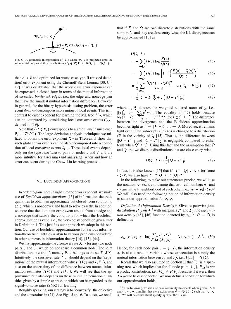
In the above theorem, which is analogous to Theorem 3.3 in[25], we derived the crossover rate as a constrained min-imization over a submanifold of distributions in (SeeFig. 5), and also proved the existence of an optimizing distri-bution . However, it is not easy to further simplify the rateexpression in (21) since the optimization is nonconvex.

Importantly, this means that it is not clear how the parametersof the distribution affect the rate ; hence, (21) is notintuitive to aid in understanding the relative ease or difficulty inestimating particular tree-structured distributions. In Section VI,we assume that satisfies some (so-called very noisy learning)conditions and use Euclidean information theory [14], [15] toapproximate the rate in (21) in order to gain insights as to howthe distribution parameters affect the crossover rate andultimately, the error exponent for learning the tree structure.

Remark 1: Theorem 2 specifies the crossover rate whenthe two node pairs and do not have any common nodes. Ifand share one node, then the distribution andhere, the crossover rate for empirical mutual information is

(23)

In Section VI, we obtain an approximate closed-form expres-sion for . The expression, provided in Theorem 8, does notdepend on whether and share a node.

Example: Symmetric Star Graph: It is now instructive tostudy a simple example to see how the overall error exponent

for structure learning in (6) depends on the set of crossoverrates . We consider a graphical model

with an associated tree which is a -order starwith a central node 1 and outer nodes , as shown inFig. 1. The edge set is given by .

We assign the joint distributions , andto the variables in this graph in the following

specific way:1) for all .2) for all , , .

Fig. 1. Star graph with � � �. � is the joint distribution on any pair ofvariables that form an edge e.g., � and � . � is the joint distribution on anypair of variables that do not form an edge e.g., � and � . By symmetry, allcrossover rates are equal.

3) for all , , , .Thus, we have identical pairwise distributions of thecentral node 1 and any other node , and also identical pairwisedistributions of any two distinct outer nodes and. Furthermore, assume that . Note that

the distribution completely specifies the abovegraphical model with a star graph. Also, from the above specifi-cations, we see that and are the marginal distributions of

with respect to to node pairs and respectivelyi.e.,

(24a)

(24b)

Note that each crossover event between any nonedge (nec-essarily of length 2) and an edge along its path results in anerror in the learned structure since it leads to being declared anedge instead of . Due to the symmetry, all such crossover ratesbetween pairs and are equal. By the “worst-exponent-wins”rule [11, Ch. 1], it is more likely to have a single crossover eventthan multiple ones. Hence, the error exponent is equal to thecrossover rate between an edge and a non-neighbor pair in thesymmetric star graph. We state this formally in the followingproposition.

Proposition 3 (Error Exponent for Symmetric Star Graph):For the symmetric graphical model with star graph and asdescribed above, the error exponent for structure learningin (6), is equal to the crossover rate between an edge and a non-neighbor node pair

for any (25)

where from (21), the crossover rate is given by

(26)with and as the marginals of , e.g.,

(27)

Proof: Since there are only two distinct distributions(which corresponds to a true edge) and (which corresponds


to a nonedge), there is only one unique rate , namely theexpression in (21) with replaced by . If the event ,in (19), occurs, an error definitely occurs. This corresponds tothe case where any one edge is replaced by any othernode pair not in .8

Hence, we have derived the error exponent for learning a sym-metric star graph through the crossover rate between anynode pair which is an edge in the star graph and another nodepair which is not an edge.

The symmetric star graph possesses symmetry in the distri-butions, and hence, it is easy to relate to a sole crossoverrate. In general, it is not straightforward to derive the error ex-ponent from the set of crossover rates since theymay not all be equal and more importantly, crossover events fordifferent node pairs affect the learned structure in a com-plex manner. In Section V, we provide an exact expression for

by identifying the (sole) crossover event related to a domi-nant error tree. Finally, we remark that the crossover eventis related to the notion of neighborhood selection in the graph-ical model learning literature [5], [8].

V. ERROR EXPONENT FOR STRUCTURE LEARNING

The analysis in the previous section characterized the ratefor the crossover event between two empirical mu-

tual information pairs. In this section, we connect these set ofrate functions to the quantity of interest, viz., the errorexponent for ML-estimation of edge set in (6).

Recall that the event denotes an error in estimating theorder of mutual information quantities. However, such events

need not necessarily lead to the error event in (5) thatthe ML-estimate of the edge set is different from the trueset . This is because the ML-estimate is a tree and thisglobal constraint implies that certain crossover events can beignored. In the sequel, we will identify useful crossover eventsthrough the notion of a dominant error tree.

A. Dominant Error Tree

We can decompose the error event for structure estimationin (5) into a set of mutually-exclusive events

(28)where each denotes the event that the graph of theML-estimate is a tree different from the true tree .In other words

ifif

(29)

Note that whenever . The large-deviation rate or the exponent for each error event is

(30)

8Also see Theorem 5 and its proof for the argument that the dominant errortree differs from the true tree by a single edge.

whenever the limit exists. Among all the error events , weidentify the dominant one with the slowest rate of decay.

Definition 1 (Dominant Error Tree): A dominant error treeis a spanning tree given by9

(31)

Roughly speaking, a dominant error tree is the tree that is themost-likely asymptotic output of the ML-estimator in the eventof an error. Hence, it belongs to the set . In the fol-lowing, we note that the error exponent in (6) is equal to theexponent of the dominant error tree.

Proposition 4 (Dominant Error Tree & Error Exponent): Theerror exponent for structure learning is equal to the expo-nent of the dominant error tree

(32)

Proof: From (30), we can write

(33)

Now from (28), we have

(34)from the “worst-exponent-wins” principle [11, Ch. 1] and thedefinition of the dominant error tree in (31).

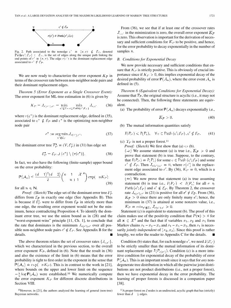
Thus, by identifying a dominant error tree , we can findthe error exponent . To this end, we revisit thecrossover events in (19), studied in the previous section.Consider a non-neighbor node pair with respect to and theunique path of edges in connecting the two nodes, which wedenote as . See Fig. 2, where we define the notionof the path given a nonedge . Note that andnecessarily form a cycle; if we replace any edge alongthe path of the non-neighbor node pair , the resulting edgeset is still a spanning tree. Hence, all suchreplacements are feasible outputs of the ML-estimation in theevent of an error. As a result, all such crossover eventsneed to be considered for the error event for structure learning

in (5). However, for the error exponent , again by the“worst-exponent-wins” principle, we only need to consider thecrossover event between each non-neighbor node pair and itsdominant replacement edge defined below.

Definition 2 (Dominant Replacement Edge): For each non-neighbor node pair , its dominant replacement edge

is defined as the edge in the unique path alongconnecting the nodes in having the minimum crossover rate

(35)

where the crossover rate is given by (21).

9We will use the notation �� extensively in the sequel. It is to be un-derstood that if there is no unique minimum (e.g., in (31)), then we arbitrarilychoose one of the minimizing solutions.


Fig. 2. Path associated to the nonedge � � �� , denoted�� , is the set of edges along the unique path linking theend points of � � �� . The edge �� is the dominant replacement edgeassociated to � �� .

We are now ready to characterize the error exponent interms of the crossover rate between non-neighbor node pairs andtheir dominant replacement edges.

Theorem 5 (Error Exponent as a Single Crossover Event):The error exponent for ML-tree estimation in (6) is given by

(36)

where is the dominant replacement edge, defined in (35),associated to and is the optimizing non-neighbornode pair

(37)

The dominant error tree in (31) has edge set

(38)

In fact, we also have the following (finite-sample) upper boundon the error probability:

(39)for all .

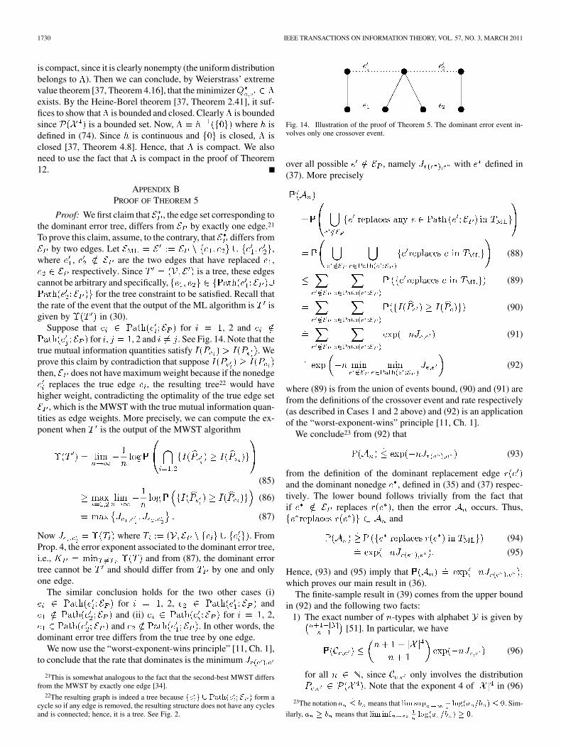
Proof: (Sketch) The edge set of the dominant error treediffers from in exactly one edge (See Appendix B). Thisis because if were to differ from in strictly more thanone edge, the resulting error exponent would not be the min-imum, hence contradicting Proposition 4. To identify the dom-inant error tree, we use the union bound as in (28) and the“worst-exponent-wins” principle [11, Ch. 1], to conclude thatthe rate that dominates is the minimum over all pos-sible non-neighbor node pairs . See Appendix B for thedetails.

The above theorem relates the set of crossover rates ,which we characterized in the previous section, to the overallerror exponent , defined in (6). Note that the result in (36)and also the existence of the limit in (6) means that the errorprobability is tight to first order in the exponent in the sense that

. This is in contrast to the work in [21],where bounds on the upper and lower limit on the sequence

were established.10 We numerically computethe error exponent for different discrete distributions inSection VIII.

10However, in [21], the authors analyzed the learning of general (non-tree)Bayesian networks.

From (36), we see that if at least one of the crossover ratesin the minimization is zero, the overall error exponent

is zero. This observation is important for the derivation of neces-sary and sufficient conditions for to be positive, and hence,for the error probability to decay exponentially in the number ofsamples .

B. Conditions for Exponential Decay

We now provide necessary and sufficient conditions that en-sure that is strictly positive. This is obviously of crucial im-portance since if , this implies exponential decay of thedesired probability of error , where the error event isdefined in (5).

Theorem 6 (Equivalent Conditions for Exponential Decay):Assume that , the original structure is acyclic (i.e., it may notbe connected). Then, the following three statements are equiv-alent.

(a) The probability of error decays exponentially i.e.,

(40)

(b) The mutual information quantities satisfy

(41)

(c) is not a proper forest.11

Proof: (Sketch) We first show that (a) (b).We assume statement (a) is true i.e., and

prove that statement (b) is true. Suppose, to the contrary,that for some and some

. Then , where is the replace-ment edge associated to . By (36), , which is acontradiction.

We now prove that statement (a) is true assumingstatement (b) is true i.e., for all

and . By Theorem 2, the crossoverrate in (21) is positive for all . From (36),

since there are only finitely many ; hence, theminimum in (37) is attained at some nonzero value, i.e.,

.Statement (c) is equivalent to statement (b). The proof of this

claim makes use of the positivity condition that forall and the fact that if variables , and formMarkov chains and , then is neces-sarily jointly independent of . Since this proof is ratherlengthy, we refer the reader to Appendix C for the details.

Condition (b) states that, for each nonedge , we needto be strictly smaller than the mutual information of its domi-nant replacement edge . Condition (c) is a more intu-itive condition for exponential decay of the probability of error

. This is an important result since it says that for any non-degenerate tree distribution in which all the pairwise joint distri-butions are not product distributions (i.e., not a proper forest),then we have exponential decay in the error probability. Thelearning of proper forests is discussed in a companion paper[38].

11A proper forest on � nodes is an undirected, acyclic graph that has (strictly)fewer than � � edges.


Fig. 3. Illustration for Example 1.

In the following example, we describe a simple randomprocess for constructing a distribution such that all threeconditions in Theorem 6 are satisfied with probability one (w.p.1). See Fig. 3.

Example 1: Suppose the structure of , a spanning tree dis-tribution with graph , is fixed and .Now, we assign the parameters of using the following proce-dure. Let be the root node. Then randomly draw the param-eter of the Bernoulli distribution from a uniform distri-bution on i.e., and .Next let be the set of neighbors of . Regard the set ofvariables as the children12 of . For each

, sample both as wellas from independent uniform dis-tributions on i.e., and .Repeat this procedure for all children of . Then repeat theprocess for all other children. This construction results in a jointdistribution for all w.p. 1. In this case, bycontinuity, all mutual informations are distinct w.p. 1, the graphis not a proper forest w.p. 1 and the rate w.p. 1.

This example demonstrates that decays exponentiallyfor almost every tree distribution.

C. Computational Complexity

Finally, we provide an upper bound on the computationalcomplexity to compute in (36). Our upper bound on thecomputational complexity depends on the diameter of the tree

which is defined as

(42)

where is the length (number of hops) of the uniquepath between nodes and . For example, for thenonedge in the subtree in Fig. 2.

Theorem 7 (Computational Complexity for ): Thenumber of computations of to compute , denoted

, satisfies

(43)

Proof: Given a non-neighbor node pair ,we perform a maximum of calculations to de-termine the dominant replacement edge from (35).Combining this with the fact that there are a total of

12Let � be the root of the tree. In general, the children of a node � �� is the set of nodes connected to � that are further away from the root than � .

Fig. 4. Partitions of the simplex associated to our learning problem are givenby � , defined in (44). In this example, the type � belongs to � so the treeassociated to partition � is favored.

nodepairs not in , we obtain the upper bound.

Thus, if the diameter of the tree is relativelylow and independent of number of nodes , the complexityis quadratic in . For instance, for a star graph, the diameter

. For a balanced tree,13 ;hence, the number of computations is .

D. Relation of the Maximum-Likelihood Structure LearningProblem to Robust Hypothesis Testing

We now take a short detour and discuss the relation betweenthe analysis of the learning problem and robust hypothesistesting, which was first considered by Huber and Strassen in[39]. Subsequent work was done in [40]–[42] albeit for differ-ently defined uncertainty classes known as moment classes.

We hereby consider an alternative but related problem.Let be the trees with nodes. Alsolet be the subsets of tree-struc-tured graphical models Markov on respectively.The structure learning problem is similar to the -ary hy-pothesis testing problem between the uncertainty classes ofdistributions . The uncertainty class denotesthe set of tree-structured graphical models with different pa-rameters (marginal and pairwise distributions

) but Markov on the same tree .In addition, we note that the probability simplex can

be partitioned into subsets14 whereeach is defined as

(44)

See Fig. 4. According to the ML criterion in (9), if the typebelongs to , then the -th tree is favored.

In [43], a subset of the authors of this paper considered theNeyman-Pearson setup of a robust binary hypothesis testingproblem where the null hypothesis corresponds to the true treemodel and the (composite) alternative hypothesis correspondsto the set of distributions Markov on some erroneous tree

. The false-alarm probability was constrained to be smaller

13A balanced tree is one where no leaf is much farther away from the rootthan any other leaf. The length of the longest direct path between any pair ofnodes is �� .

14From the definition in (44), we see that the relative interior of the subsetsare pairwise disjoint. We discuss the scenario when � lies on the boundaries ofthese subsets in Section VII.


Fig. 5. A geometric interpretation of (21) where � is projected onto thesubmanifold of probability distributions �� .

than and optimized for worst-case type-II (missed detec-tion) error exponent using the Chernoff-Stein Lemma [30, Ch.12]. It was established that the worst-case error exponent canbe expressed in closed-form in terms of the mutual informationof so-called bottleneck edges, i.e., the edge and nonedge pairthat have the smallest mutual information difference. However,in general, for the binary hypothesis testing problem, the errorevent does not decompose into a union of local events. This is incontrast to error exponent for learning the ML tree , whichcan be computed by considering local crossover events ,defined in (19).

Note that corresponds to a global event since each. The large-deviation analysis techniques we uti-

lized to obtain the error exponent in Theorem 5 show thatsuch global error events can be also decomposed into a collec-tion of local crossover events . These local events dependonly on the type restricted to pairs of nodes and and aremore intuitive for assessing (and analyzing) when and how anerror can occur during the Chow-Liu learning process.

VI. EUCLIDEAN APPROXIMATIONS

In order to gain more insight into the error exponent, we makeuse of Euclidean approximations [15] of information-theoreticquantities to obtain an approximate but closed-form solution to(21), which is nonconvex and hard to solve exactly. In addition,we note that the dominant error event results from an edge anda nonedge that satisfy the conditions for which the Euclideanapproximation is valid, i.e., the very-noisy condition given laterin Definition 4. This justifies our approach we adopt in this sec-tion. Our use of Euclidean approximations for various informa-tion-theoretic quantities is akin to various problems consideredin other contexts in information theory [14], [15], [44].

We first approximate the crossover rate for any two nodepairs and , which do not share a common node. The jointdistribution on and , namely belongs to the set .Intuitively, the crossover rate should depend on the “sepa-ration” of the mutual information values and , andalso on the uncertainty of the difference between mutual infor-mation estimates and . We will see that the ap-proximate rate also depends on these mutual information quan-tities given by a simple expression which can be regarded as thesignal-to-noise ratio (SNR) for learning.

Roughly speaking, our strategy is to “convexify” the objectiveand the constraints in (21). See Figs. 5 and 6. To do so, we recall

that if and are two discrete distributions with the samesupport , and they are close entry-wise, the KL divergence canbe approximated [15] as

(45)

(46)

(47)

(48)

where denotes the weighted squared norm of , i.e.,. The equality in (47) holds because

for . The differencebetween the divergence and the Euclidean approximationbecomes tight as . Moreover, it remainstight even if the subscript in (48) is changed to a distribution

in the vicinity of [15]. That is, the difference betweenand is negligible compared to either

term when . Using this fact and the assumption thatand are two discrete distributions that are close entry-wise

(49)

In fact, it is also known [15] that if for some, we also have .

In the following, to make our statements precise, we will usethe notation to denote that two real numbers and

are in the neighborhood of each other, i.e., .15

We will also need the following notion of information densityto state our approximation for .

Definition 3 (Information Density): Given a pairwise jointdistribution on with marginals and , the informa-tion density [45], [46] function, denoted by , isdefined as

(50)

Hence, for each node pair , the information densityis also a random variable whose expectation is simply the

mutual information between and , i.e., .Recall that we also assumed in Section II that is a span-

ning tree, which implies that for all node pairs , is nota product distribution, i.e., , because if it were, then

would be disconnected. We now define a condition for whichour approximation holds.

15In the following, we will also have continuity statements where given � � �and � � � , implies that there exists some � � �� such that � �� . We will be casual about specifying what the �’s are.


Definition 4 ( -Very Noisy Condition): We say that, the joint distribution on node pairs and , satisfies

the -very noisy condition if

(51)

This condition is needed because if (51) holds, then by conti-nuity of the mutual information, there exists a such that

, which means that the mutual informationquantities are difficult to distinguish and the approximation in(48) is accurate.16 Note that proximity of the mutual informa-tion values is not sufficient for the approximation to hold sincewe have seen from Theorem 2 that depends not only on themutual information quantities but on the entire joint distribution

.We now define the approximate crossover rate on disjoint

node pairs and as

(52)

where the (linearized) constraint set is

(53)

where is the gradient vector of the mutual infor-mation with respect to the joint distribution , regarded as alength- vector. We also define the approximate error expo-nent as

(54)

We now provide the expression for the approximate crossoverrate and also state the conditions under which the approx-imation is asymptotically accurate in .17

Theorem 8 (Euclidean Approximation of ): The approx-imate crossover rate for the empirical mutual information quan-tities, defined in (52), is given by

(55)

where is the information density defined in (50) and the ex-pectation and variance are both with respect to . Further-more, the approximation (55) is asymptotically accurate, i.e., as

(in the definition of -very noisy condition), we have that.

16Here and in the following, we do not specify the exact value of � but wesimply note that as �� , the approximation in (49) becomes tighter.

17We say that a collection of approximations �� of a true param-eter � is asymptotically accurate in � (or simply asymptotically accurate) if theapproximations converge to � as �� , i.e., �� .

Proof: (Sketch) (52) and (53) together define a least squaresproblem. Upon simiplification of the solution, we obtain (55).See Appendix D for the details.

We also have an additional result for the Euclidean approx-imation for the overall error exponent . The proof is clearfrom the definition of in (54) and the continuity of the minfunction.

Corollary 9 (Euclidean Approximation of ): The approx-imate error exponent is asymptotically accurate if all jointdistributions in the set sat-isfy the -very noisy condition.

Hence, the expressions for the crossover rate and theerror exponent are vastly simplified under the -very noisycondition on the joint distributions . The approximatecrossover rate in (55) has a very intuitive meaning. It isproportional to the square of the difference between the mutualinformation quantities of and . This corresponds exactlyto our initial intuition—that if and are well sepa-rated then the crossover rate has to be large.

is also weighted by the precision (inverse variance) of. If this variance is large then we are uncertain about

the estimate , and crossovers are more likely,thereby reducing the crossover rate .

We now comment on our assumption of satisfying the-very noisy condition, under which the approximation is tight

as seen in Theorem 8. When is -very noisy, then wehave , which implies that the optimal solution

. When is an edge and is a non-neighbornode pair, this implies that it is very hard to distinguish the rela-tive magnitudes of the empiricals and . Hence, theparticular problem of learning the distribution from sam-ples is very noisy. Under these conditions, the approximation in(55) is accurate.

In summary, our approximation in (55) takes into accountnot only the absolute difference between the mutual informa-tion quantities and , but also the uncertainty inlearning them. The expression in (55) is, in fact, the SNR forthe estimation of the difference between empirical mutual infor-mation quantities. This answers one of the fundamental ques-tions we posed in the introduction, viz., that we are now ableto distinguish between distributions that are “easy” to learn andthose that are “difficult” by computing the set of SNR quantities

in (55).

VII. EXTENSIONS TO NON-TREE DISTRIBUTIONS

In all the preceding sections, we dealt exclusively with thecase where the true distribution is Markov on a tree. In thissection, we extend the preceding large-deviation analysis to dealwith distributions that may not be tree-structured but in whichwe estimate a tree distribution from the given set of samples

, using the Chow-Liu ML-estimation procedure. Since theChow-Liu procedure outputs a tree, it is not possible to learn thestructure of correctly. Hence, it will be necessary to redefinethe error event.


Fig. 6. Convexifying the objective results in a least-squares problem. The ob-jective is converted into a quadratic as in (52) and the linearized constraint set�� is given (53).

Fig. 7. Reverse I-projection [13] of � onto the set of tree distributions�� given by (56).

TABLE ITABLE OF PROBABILITY VALUES FOR EXAMPLE 2

When is not a tree distribution, we analyze the propertiesof the optimal reverse I-projection [13] of onto the set of treedistributions, given by the optimization problem18

(56)

is the KL-divergence of to the closest element in. See Fig. 7. As Chow and Wagner [10] noted, if

is not a tree, there may be several trees optimizing (56).19 Wedenote the set of optimal projections as , given by

(57)

We now illustrate that may have more than one ele-ment with the following example.

Example 2: Consider the parameterized discrete proba-bility distribution shown in Table I where

and are constants.

Proposition 10 (Nonuniqueness of Projection): For suffi-ciently small , the Chow-Liu MWST algorithm (using either

18The minimum in the optimization problem in (56) is attained because theKL-divergence is continuous and the set of tree distributions �� iscompact.

19This is a technical condition of theoretical interest in this section. In fact, itcan be shown that the set of distributions such that there is more than one treeoptimizing (56) has ( � �-Lebesgue) measure zero in �� .

Fig. 8. Each tree defines an �-flat submanifold [47], [48] of probability distri-butions. These are the two lines as shown in the figure. If the KL-divergences�� and �� are equal, then � and � do not have thesame structure but both are optimal with respect to the optimization problem in(56). An example of such a distribution � is provided in Example 2.

Kruskal’s [35] or Prim’s [36] procedure) will first include theedge (1, 2). Then, it will arbitrarily choose between the tworemaining edges (2, 3) or (1, 3).

The proof of this proposition is provided in Appendix Ewhere we show that for suf-ficiently small . Thus, the optimal tree structure is notunique. This in fact corresponds to the case where belongsto the boundary of some set defined in (44). SeeFig. 8 for an information geometric interpretation.

Every tree distribution in has the maximum sum mu-tual information weight. More precisely, we have

(58)

Given (58), we note that when we use a MWST algorithm tofind the optimal solution to the problem in (56), ties will be en-countered during the greedy addition of edges, as demonstratedin Example 2. Upon breaking the ties arbitrarily, we obtain somedistribution . We now provide a sequence of usefuldefinitions that lead to definition of a new error event for whichwe can perform large-deviation analysis.

We denote the set of tree structures20 corresponding to thedistributions in as

(59)

and term it as the set of optimal tree projections. A similar def-inition applies to the edge sets of optimal tree projections

(60)

Since the distribution is unknown, our goal is to estimatethe optimal tree-projection using the empirical distribution

, where is given by

(61)

If there are many distributions , we arbitrarily pick one ofthem. We will see that by redefining the error event, we will havestill a LDP. Finding the reverse I-projection can be solvedefficiently (in time ) using the Chow-Liu algorithm[3] as described in Section III.

20In fact, each tree defines a so-called e-flat submanifold [47], [48] inthe set of probability distributions on � and � lies in both submani-folds. The so-called m-geodesic connects � to any of its optimal projection� � � �� .


We define as the graph of , which isthe learned tree and redefine the new error event as

(62)

Note that this new error event essentially reduces to the originalerror event in (5) if contains only onemember. So if the learned structure belongs to , there isno error, otherwise an error is declared. We would like to analyzethe decay of the error probability of as defined in(62), i.e., find the new error exponent

(63)

It turns out that the analysis of the new event is verysimilar to the analysis performed in Section V. We redefine thenotion of a dominant replacement edge and the computation ofthe new rate then follows automatically.

Definition 5 (Dominant Replacement Edge): Fix an edge set. For the error event defined in (62),

given a non-neighbor node pair , its dominant replace-ment edge with respect to , is given by

(64)

if there exists an edge such that. Otherwise . is the crossover

rate of mutual information quantities defined in (20). Ifexists, the corresponding crossover rate is

(65)

otherwise .In (64), we are basically fixing an edge set and

excluding the trees with replaced by if itbelongs to the set of optimal tree projections . We fur-ther remark that in (64), may not necessarily exist. Indeed,this occurs if every tree with replaced bybelongs to the set of optimal tree projections. This is, however,not an error by the definition of the error event in (62); hence, weset . In addition, we define the dominant nonedgeassociated to edge set as

(66)

Also, the dominant structure in the set of optimal tree projec-tions is defined as

(67)

where the crossover rate is defined in (65) and thedominant nonedge associated to is defined in (66).Equipped with these definitions, we are now ready to state thegeneralization of Theorem 5.

Theorem 11 (Dominant Error Tree): For the error eventdefined in (62), a dominant error tree (which may

not be unique) has edge set given by

(68)

where is the dominant nonedge associated to thedominant structure and is defined by (66) and(67). Furthermore, the error exponent , defined in (63)is given as

(69)

Proof: The proof of this theorem follows directly by iden-tifying the dominant error tree belonging to the set .By further applying the result in Proposition 4 and Theorem 5,we obtain the result via the “worst-exponent-wins” [11, Ch. 1]principle by minimizing over all trees in the set of optimal pro-jections in (69).

This theorem now allows us to analyze the more general errorevent , which includes in (5) as a special case ifthe set of optimal tree projections in (59) is a singleton.

VIII. NUMERICAL EXPERIMENTS

In this section, we perform a series of numerical experimentswith the following three objectives:

1) In Section VIII-A, we study the accuracy of the Euclideanapproximations (Theorem 8). We do this by analyzingunder which regimes the approximate crossover ratein (55) is close to the true crossover rate in (21).

2) Since the LDP and error exponent analysis are asymptotictheories, in Section VIII-B we use simulations to studythe behavior of the actual crossover rate, given a finitenumber of samples . In particular, we study how fast thecrossover rate, obtained from simulations, converges to thetrue crossover rate. To do so, we generate a number of sam-ples from the true distribution and use the Chow-Liu algo-rithm to learn trees structures. Then we compare the resultto the true structure and finally compute the error proba-bility.

3) In Section VIII-C, we address the issue of the learnernot having access to the true distribution, but nonethelesswanting to compute an estimate of the crossover rate.The learner only has the samples or equivalently, theempirical distribution . However, in all the precedinganalysis, to compute the true crossover rate and theoverall error exponent , we used the true distributionand solved the constrained optimization problem in (21).Alternatively we computed the approximation in (55),which is also a function of the true distribution. However,in practice, it is also useful to compute an online estimateof the crossover rate by using the empirical distribution inplace of the true distribution in the constrained optimiza-tion problem in (21). This is an estimate of the rate that thelearner can compute given the samples. We call this theempirical rate and formally define it in Section VIII-C.


Fig. 9. Graphical model used for our numerical experiments. The true modelis a symmetric star (cf. Section IV) in which the mutual information quantitiessatisfy �� and by construction, �� for any nonedge � . Besides, the mutual information quantities on the nonedgesare equal, for example, �� .

We perform convergence analysis of the empirical rateand also numerically verify the rate of convergence to thetrue crossover rate.

In the following, we will be performing numerical experi-ments for the undirected graphical model with four nodes asshown in Fig. 9. We parameterize the distribution withvariables with a single parameter and let , i.e.,all the variables are binary. For the parameters, we set

and

(70a)

(70b)

With this parameterization, we see that if is small, the mu-tual information for , 3, 4 is also small. In fact if

, is independent of for , 3, 4 and as a result,. Conversely, if is large, the mutual information

increases as the dependence of the outer nodes with thecentral node increases. Thus, we can vary the size of the mutualinformation along the edges by varying . By symmetry, thereis only one crossover rate, and hence, this crossover rate is alsothe error exponent for the error event in (5). This is exactlythe same as the symmetric star graph as described in Section IV.

A. Accuracy of Euclidean Approximations

We first study the accuracy of the Euclidean approximationsused to derive the result in Theorem 8. We denote the true rateas the crossover rate resulting from the nonconvex optimiza-tion problem (21) and the approximate rate as the crossover ratecomputed using the approximation in (55).

We vary from 0 to 0.2 and plot both the true and approx-imate rates against the difference between the mutual informa-tions in Fig. 10, where denotes any edge and

denotes any nonedge in the model. The nonconvex optimiza-tion problem was performed using the Matlab functionin the optimization toolbox. We used several different feasiblestarting points and chose the best optimal objective value toavoid problems with local minima. We first note from Fig. 10that both rates increase as increases. This is inline with our intuition because if is such thatis large, the crossover rate is also large. We also observe that if

is small, the true and approximate rates are veryclose. This is in line with the assumptions for Theorem 8. Recall

Fig. 10. Comparison of true and approximate rates.

that if satisfies the -very noisy condition (for some small), then the mutual information quantities and are

close and consequently the true and approximate crossover ratesare also close. When the difference between the mutual infor-mations increases, the true and approximate rate separate fromeach other.

B. Comparison of True Crossover Rate to the Rate ObtainedFrom Simulations

In this section, we compare the true crossover rate in (21) tothe rate we obtain when we learn tree structures using Chow-Liuwith i.i.d. samples drawn from , which we define as the sim-ulated rate. We fixed in (70) then for each , we esti-mated the probability of error using the Chow-Liu algorithm asdescribed in Section III. We state the procedure precisely in thefollowing steps.

1) Fix and sample i.i.d. observations from .2) Compute the empirical distribution and the set of empir-

ical mutual information quantities .3) Learn the Chow-Liu tree using a MWST algorithm

with as the edge weights.4) If is not equal to , then we declare an error.5) Repeat steps 1–4 a total of times and estimate the

probability of error and the errorexponent , which is the simulated rate.

If the probability of error is very small, then the numberof runs to estimate has to be fairly large. This is oftenthe case in error exponent analysis as the sample size needs tobe substantial to estimate very small error probabilities.

In Fig. 11, we plot the true rate, the approximate rate and thesimulated rate when (and ) and(and ). Note that, in the former case, the truerate is higher than the approximate rate and in the latter case,the reverse is true. When is large , there are largedifferences in the true tree models. Thus, we expect that the errorprobabilities to be very small, and hence, has to be large inorder to estimate the error probability correctly but does nothave to be too large for the simulated rate to converge to the truerate. On the other hand, when is small , there areonly subtle differences in the graphical models; hence, we need


Fig. 11. Comparison of true, approximate and simulated rates with � � ��(top) and � � �� (bottom). Here the number of runs � � �� for � � ��

and � � �� for � � ��. The probability of error is computed dividingthe total number of errors by the total number of runs.

a larger number of samples for the simulated rate to convergeto its true value, but does not have to be large since the errorprobabilities are not small. The above observations are in linewith our intuition.

C. Comparison of True Crossover Rate to Rate Obtained Fromthe Empirical Distribution

In this subsection, we compare the true rate to the empiricalrate, which is defined as

(71)

The empirical rate is a function of theempirical distribution . This rate is computable by alearner, who does not have access to the true distribution .The learner only has access to a finite number of samples

. Given , the learner can compute theempirical probability and perform the optimization in(71). This is an estimate of the true crossover rate. A naturalquestion to ask is the following: Does the empirical rateconverge to the true crossover rate as ? The nexttheorem answers this question in the affirmative.

Theorem 12 (Crossover Rate Consistency): The empiricalcrossover rate in (71) converges almost surely to the truecrossover rate in (21), i.e.,

(72)

Fig. 12. Comparison of True, Approximate and Empirical Rates with � � ��(top) and � � �� (bottom). Here � is the number of observations used toestimate the empirical distribution.

Proof: (Sketch) The proof of this theorem follows fromthe continuity of in the empirical distribution andthe continuous mapping theorem by Mann and Wald [49]. SeeAppendix F for the details.

We conclude that the learning of the rate from samples isstrongly consistent. Now we perform simulations to determinehow many samples are required for the empirical rate to con-verge to the true rate.

We set and in (70). We then drewi.i.d. samples from and computed the empirical distribution

. Next, we solved the optimization problem in (71) usingthe function in Matlab, using different initializationsand compared the empirical rate to the true rate. We repeated thisfor several values of and the results are displayed in Fig. 12.We see that for , approximately samplesare required for the empirical distribution to be close enough tothe true distribution so that the empirical rate converges to thetrue rate.

IX. CONCLUSION, EXTENSIONS AND OPEN PROBLEMS

In this paper, we presented a solution to the problem offinding the error exponent for tree structure learning by exten-sively using tools from large-deviations theory combined withfacts about tree graphs. We quantified the error exponent forlearning the structure and exploited the structure of the truetree to identify the dominant tree in the set of erroneous trees.We also drew insights from the approximate crossover rate,which can be interpreted as the SNR for learning. These two


main results in Theorems 5 and 8 provide the intuition as tohow errors occur for learning discrete tree distributions via theChow-Liu algorithm.

In a companion paper [27], we develop counterparts to theresults here for the Gaussian case. Many of the results carrythrough but thanks to the special structure that Gaussian distri-butions possess, we are also able to identify which structures(among the class of trees) are easier to learn and which areharder to learn given a fixed set of correlation coefficients on theedges. Using Euclidean information theory, we show that if theparameters on the edges are fixed, the star is the most difficultto learn (requiring many more samples to ensure )while the Markov chain is the easiest. The results in this paperhave also been extended to learning high-dimensional generalacyclic models (forests) [38], where grows with and typi-cally the growth of is much faster than that of .

There are many open problems resulting from this paper. Oneof these involves studying the optimality of the error exponentassociated to the ML Chow-Liu algorithm , i.e., whether therate established in Theorem 5 is the best (largest) among allconsistent estimators of the edge set. Also, since large-deviationrates may not be indicative of the true error probability ,results from weak convergence theory [50] may potentially beapplicable to provide better approximations to .

APPENDIX APROOF OF THEOREM 2

Proof: We divide the proof of this theorem into three steps.Steps 1 and 2 prove the expression in (21). Step 3 proves theexistence of the optimizer.

Step 1: First, we note from Sanov’s Theorem [30, Ch. 11]that the empirical joint distribution on edges and satisfies

(73)for any set that equals the closure of its inte-rior, i.e., . We now have a LDP for the se-quence of probability measures , the empirical distributionon . Assuming that and do not share a common node,

is a probability distribution over four variables(the variables in the node pairs and ). We now define thefunction as

(74)

Since , defined in (22) is continuous in andthe mutual information is also continuous in , we con-clude that is indeed continuous, since it is the composition ofcontinuous functions. By applying the contraction principle [11]to the sequence of probability measures and the continuousmap , we obtain a corresponding LDP for the new sequence ofprobability measures , where the rateis given by

(75)

(76)

Fig. 13. Illustration of Step 2 of the proof of Theorem 2.

We now claim that the limit in (20) exists. From Sanov’s the-orem [30, Ch. 11], it suffices to show that the constraint set

in (76) is a regular closed set, i.e.,it satisfies . This is true because there are noisolated points in , and, thus, the interior is nonempty. Hence,there exists a sequence of distributionssuch that , which provesthe existence of the limit in (20).

Step 2: We now show that the optimal solution ,if it exists (as will be shown in Step 3), must satisfy

. Suppose, to the contrary, that withobjective value is such that .Then , where , as shown above, is continuous.Thus, there exists a such that the -neighborhood

(77)

satisfies [37, Ch. 2]. Consider the newdistribution (See Fig. 13)

(78)

(79)

Note that belongs to , and hence, is a fea-sible solution of (76). We now prove that

, which contradicts the optimality of .

(80)

(81)

(82)

(83)

where (81) is due to the convexity of the KL-divergence in thefirst variable [30, Ch. 2], (82) is becauseand (83) is because . Thus, we conclude that the optimalsolution must satisfy and the crossover ratecan be stated as (21).

Step 3: Now, we prove the existence of the minimizer, which will allow us to replace the in (21) with min.

First, we note that is continuous in both variables,and hence continuous and the first variable . It remains toshow that the constraint set

(84)


is compact, since it is clearly nonempty (the uniform distributionbelongs to ). Then we can conclude, by Weierstrass’ extremevalue theorem [37, Theorem 4.16], that the minimizerexists. By the Heine-Borel theorem [37, Theorem 2.41], it suf-fices to show that is bounded and closed. Clearly is boundedsince is a bounded set. Now, where isdefined in (74). Since is continuous and is closed, isclosed [37, Theorem 4.8]. Hence, that is compact. We alsoneed to use the fact that is compact in the proof of Theorem12.

APPENDIX BPROOF OF THEOREM 5

Proof: We first claim that , the edge set corresponding tothe dominant error tree, differs from by exactly one edge.21

To prove this claim, assume, to the contrary, that differs fromby two edges. Let ,

where , are the two edges that have replaced ,respectively. Since is a tree, these edges

cannot be arbitrary and specifically,for the tree constraint to be satisfied. Recall that

the rate of the event that the output of the ML algorithm is isgiven by in (30).

Suppose that for , 2 andfor , , 2 and . See Fig. 14. Note that the

true mutual information quantities satisfy . Weprove this claim by contradiction that supposethen, does not have maximum weight because if the nonedge

replaces the true edge , the resulting tree22 would havehigher weight, contradicting the optimality of the true edge set

, which is the MWST with the true mutual information quan-tities as edge weights. More precisely, we can compute the ex-ponent when is the output of the MWST algorithm

(85)

(86)

(87)

Now where . FromProp. 4, the error exponent associated to the dominant error tree,i.e., and from (87), the dominant errortree cannot be and should differ from by one and onlyone edge.

The similar conclusion holds for the two other cases (i)for , 2, andand (ii) for , 2,

and . In other words, thedominant error tree differs from the true tree by one edge.

We now use the “worst-exponent-wins principle” [11, Ch. 1],to conclude that the rate that dominates is the minimum

21This is somewhat analogous to the fact that the second-best MWST differsfrom the MWST by exactly one edge [34].

22The resulting graph is indeed a tree because �� form acycle so if any edge is removed, the resulting structure does not have any cyclesand is connected; hence, it is a tree. See Fig. 2.

Fig. 14. Illustration of the proof of Theorem 5. The dominant error event in-volves only one crossover event.

over all possible , namely with defined in(37). More precisely

(88)

(89)

(90)

(91)

(92)

where (89) is from the union of events bound, (90) and (91) arefrom the definitions of the crossover event and rate respectively(as described in Cases 1 and 2 above) and (92) is an applicationof the “worst-exponent-wins” principle [11, Ch. 1].

We conclude23 from (92) that

(93)

from the definition of the dominant replacement edgeand the dominant nonedge , defined in (35) and (37) respec-tively. The lower bound follows trivially from the fact thatif replaces , then the error occurs. Thus,

and

(94)

(95)

Hence, (93) and (95) imply thatwhich proves our main result in (36).

The finite-sample result in (39) comes from the upper boundin (92) and the following two facts:

1) The exact number of -types with alphabet is given by[51]. In particular, we have

(96)

for all , since only involves the distribution. Note that the exponent 4 of in (96)

23The notation � � � means that � �� . Sim-

ilarly, � � � means that � �� .


is an upper bound since if and share a node.

2) The number of error events is at mostbecause there are nonedgesand for each nonedge, there are at most edges alongits path.

This completes the proof.

APPENDIX CPROOF OF THEOREM 6

Statement (a) statement (b) was proven in full after thetheorem was stated. Here we provide the proof that (b) (c).Recall that statement (c) says that is not a proper forest. Wefirst begin with a preliminary lemma.

Lemma 13: Suppose , , are three random variablestaking on values on finite sets , , respectively. Assumethat everywhere. Then andare Markov chains if and only if is jointly independent of , .

Proof: That is a Markov chain implies that

(97)

or alternatively

(98)

Similarly from the fact that is a Markov chain, wehave

(99)

Equating (98) and (99), and use the positivity to cancel ,we arrive at

(100)

It follows that does not depend on , so there is someconstant such that for all . Thisimmediately implies that so that .A similar argument gives that . Furthermore, if

is a Markov chain, so is , therefore

(101)

The above equation says that is jointly independent of bothand .

Conversely, if is jointly independent of both and ,then and are Markov chains. In fact is notconnected to .

Proof: We now prove (b) (c) using Lemma 13 andthe assumption that for all .

If (b) is true then for alland for all . Assume, to the contrary, that

is a proper forest, i.e., it contains at least 2 connected com-ponents (each connected component may only have one node),say for , 2. Without loss of generality, letbe in component and , belong to component . Then

since and , we have that jointlyindependent of and . By Lemma 13, we have the followingMarkov chains and . This impliesfrom the Data Processing Inequality [30, Theorem 2.8.1] that

and at the same timewhich means that . This contradicts (b) sinceby taking , the mutual informations along the path

are no longer distinct.Now assume that (c) is true, i.e., is not a proper forest.

Suppose, to the contrary, (b) is not true, i.e., there exists asuch that , where is the replacement

edge associated with the nonedge . Without loss of generality,let and , then since is not a properforest, we have the following Markov chain .Now note that . In fact, because there is noloss of mutual information , and hence, bythe Data Processing Inequality, we also have .By using Lemma 13, we have jointly independent of and

; hence, we have a proper forest, which is a contradiction.

APPENDIX DPROOF OF THEOREM 8

Proof: The proof proceeds in several steps. See Figs. 5 and6 for intuition behind this proof.

Step 1: Let be such that

(102)

Thus, the ’s are the deviations of from . To ensurethat is a valid distribution we require . Theobjective in (52) can now be alternatively expressed as

(103)

where is the vectorized version of the deviationsand is a diagonal matrix containing

the entries along its diagonal.Step 2: We now perform a first-order Taylor expansion of

in the neighborhood of .

(104)

(105)

where is the length -vector that contains the informationdensity values of edge . Note that because of the assumptionthat is not a proper forest, for all ; hence,the linear term does not vanish.24 The constraints can now berewritten as

(106)

or in matrix notation as

(107)

24Indeed if � were a product distribution, the linear term in (105) vanishesand �� is approximately a quadratic in �� (as shown in [15]).


where is the length- vector consisting of all ones. Forconvenience, we define to be the matrix in (107) i.e.,

(108)

Step 3: The optimization problem now reduces to mini-mizing (103) subject to the constraints in (107). This is a stan-dard least-squares problem. By using the Projection Theorem inHilbert spaces (or Lagrange multipliers), we get the solution

(109)The inverse of exists because we assumedis not a proper forest, and hence, for all

. This is a sufficient condition for the matrix to havefull row rank and thus, is invertible. Finally, wesubstitute in (109) into (103) to obtain

(110)

where is the (1,1) element of the matrix . Define tobe the weighting function given by

(111)

It now suffices to show that is indeed the inversevariance of . We now simplify the expression for theweighting function recalling how and aredefined. The product of the matrices in (111) is

(112)

where all expectations are with respect to the distribution .Note that the determinant of (112) is

. Hence, the (1,1) element of the inverseof (112) is simply

(113)

Now, if and share a node, this proof proceeds in exactly thesame way. In particular, the crucial step (105) will also remainthe same since the Taylor expansion does not change. This con-cludes the first part of the proof.

Step 4: We now prove the continuity statement. The ideais that all the approximations become increasingly exact as (inthe definition of the -very noisy condition) tends to zero. Moreconcretely, for every , there exists a such that if

satisfies the -very noisy condition, then

(114)

since mutual information is continuous. For every , thereexists a such that if satisfies the -very noisycondition, then

(115)

since if is -very noisy it is close to the constraint set, and hence, close to the optimal solution

. For every , there exists a such that ifsatisfies the -very noisy condition, then

(116)

which follows from the approximation of the divergence andthe continuity statement in (115). For every , there existsa such that if satisfies the -very noisy condition,then

(117)

which follows from retaining only the first term in the Taylorexpansion of the mutual information in (105). Finally, for every

, there exists a such that if satisfies the -verynoisy condition, then

(118)

which follows from continuity of the objective in the constraints(117). Now choose to conclude that for every

, there exists a such that if satisfies the -verynoisy condition, then (118) holds. This completes the proof.

APPENDIX EPROOF OF PROPOSITION 10

Proof: The following facts about in Table I can bereadily verified:

1) is positive everywhere, i.e., for all .2) is Markov on the complete graph with nodes;

hence, is not a tree-structured distribution.3) The mutual information between and as a function

of is given by

Thus, as .4) For any ,

and this pair of mutual information quantities can be madearbitrarily small as .

Thus, for sufficiently small ,. We conclude that the Chow-Liu MWST algorithm will

first pick the edge (1, 2) and then arbitrarily choose between thetwo remaining edges: (2, 3) or (1, 3). Thus, optimal tree struc-ture is not unique.

APPENDIX FPROOF OF THEOREM 12

We first state two preliminary lemmas and prove the first one.Theorem 12 will then be an immediate consequence of theselemmas.

Lemma 14: Let and be two metric spaces and letbe a compact set in . Let be a


continuous real-valued function. Then the function ,defined as

(119)

is continuous on .Proof: Set the minimizer in (119) to be

(120)

The optimizer exists since is continuous onfor each and is compact. This follows from Weier-

strass’ extreme value theorem [37, Theorem 4.16]. We want toshow that for . In other words, we need toprove that

(121)

Consider the difference

(122)

The first term in (122) tends to zero as by thecontinuity of so it remains to show that the second term,

, as . Now, wecan remove the absolute value since by the optimality of ,

. Hence

(123)

Suppose, to the contrary, there exists a sequencewith such that

(124)

By the compactness of , for the sequence ,there exists a subsequence whose limit is

and [37, Theorem 3.6(a)]. Bythe continuity of

(125)

(126)

since every subsequence of a convergent sequence con-verges to the same limit . Now (124) can be written as

(127)

We now take the limit as of (127). Next, we use (125)and (126) to conclude that

(128)

which contradicts the optimality of in (120). Thus,as and , which demonstrates the

continuity of on .

Lemma 15 (The Continuous Mapping Theorem [49]):Let be a probability space. Let the sequence ofrandom variables on converge -almost surely

to , i.e., . Let be a continuousfunction. Then converges -almost surely to , i.e.,

.Proof: Now, using Lemmas 14 and 15, we complete the

proof of Theorem 12. First we note from (71) that, i.e., is a function of the empirical distribu-

tion on node pairs and . Next, we note that is acontinuous function in . If is fixed, the expres-sion (71) is a minimization of , over the compactset25 ; hence, Lemma 14applies (with the identifications and ) which im-plies that is continuous in the empirical distribution .Since the empirical distribution converges almost surely to

[30, Sec. 11.2], also converges almost surelyto , by Lemma 15.

ACKNOWLEDGMENT

The authors would like to thank the anonymous referees andAssociate Editor A. Krzyzak who have helped to improve theexposition. One reviewer, in particular, helped highlight theconnection of this work with robust hypothesis testing, leadingto Section V-D. The authors would also like to thank Prof. L.Zheng, M. Agrawal, and A. Olshevsky for many stimulatingdiscussions.

REFERENCES

[1] V. Y. F. Tan, A. Anandkumar, L. Tong, and A. S. Willsky, “A large-de-viation analysis for the maximum likelihood learning of tree struc-tures,” in Proc. IEEE Int. Symp. Information Theory, Seoul, Korea, Jul.2009, pp. 1140–1144.

[2] S. Lauritzen, Graphical Models. Oxford, U,K,: Oxford Univ. Press,1996.

[3] C. K. Chow and C. N. Liu, “Approximating discrete probability distri-butions with dependence trees,” IEEE Trans. Inf. Theory, vol. IT-14,no. 3, pp. 462–467, May 1968.

[4] A. Chechetka and C. Guestrin, “Efficient principled learning of thinjunction trees,” presented at the Neural Inf. Process. Syst., 2007.

[5] M. J. Wainwright, P. Ravikumar, and J. D. Lafferty, “High-dimen-sional graphical model selection using -regularized logistic regression,”in Neural Information Processing Systems. Cambridge, MA: MITPress, 2006, pp. 1465–1472.

[6] S. Lee, V. Ganapathi, and D. Koller, “Efficient structure learning ofMarkov networks using � -regularization,” presented at the Neural Inf.Process. Syst., 2006.

[7] J. Johnson, V. Chandrasekaran, and A. S. Willsky, “Learning Markovstructure by maximum entropy relaxation,” presented at the ArtificialIntelligence and Statistics (AISTATS), 2007.

[8] N. Meinshausen and P. Buehlmann, “High-dimensional graphs andvariable selection with the Lasso,” Ann. Statist., vol. 34, no. 3, pp.1436–1462, Jun 2006.

[9] M. Dudik, S. Phillips, and R. Schapire, “Performance guarantees forregularized maximum entropy density estimation,” presented at theConf. Learning Theor. (COLT), 2004.

[10] C. K. Chow and T. Wagner, “Consistency of an estimate of tree-depen-dent probability distributions,” IEEE Trans. Inf. Theory, vol. IT-19, no.3, pp. 369–371, May 1973.

[11] F. D. Hollander, Large Deviations (Fields Institute Monographs,14). Providence, RI: AMS, 2000.

[12] D. B. West, Introduction to Graph Theory, 2nd ed. Englewood Cliffs,NJ: Prentice-Hall, 2000.

[13] I. Csiszár and F. Matús, “Information projections revisited,” IEEETrans. Inf. Theory, vol. 49, no. 6, pp. 1474–1490, Jun. 2003.

[14] S. Borade and L. Zheng, “I-projection and the geometry of error ex-ponents,” presented at the Allerton Conf. Communication, Control,Comput., 2006.

[15] S. Borade and L. Zheng, “Euclidean information theory,” presented atthe Allerton Conf. Communication, Control, Comput., 2007.

25Compactness of � was proven in Theorem 2 cf. Equation (84).


[16] D. Karger and N. Srebro, “Learning Markov networks: Maximumbounded tree-width graphs,” in Proc. Symp. Discrete Algorithms,2001, pp. 392–401.

[17] F. Bach and M. I. Jordan, “Thin junction trees,” presented at the NeuralInf. Process. Syst., 2002.

[18] D. Heckerman and D. Geiger, Learning Bayesian networks, MicrosoftResearch, Redmond, WA, 1994, Tech. Rep. MSR-TR-95-02.

[19] G. Schwarz, “Estimating the dimension of a model,” Ann. Statist., vol.6, no. 2, pp. 461–464, 1978.

[20] R. Tibshirani, “Regression shrinkage and selection via the Lasso,” J.Roy. Statist. Soc. B, vol. 58, no. 1, pp. 267–288, 1996.

[21] O. Zuk, S. Margel, and E. Domany, “On the number of samples neededto learn the correct structure of a Bayesian network,” presented at the22nd Annu. Conf. Uncertainty Artificial Intell. (UAI-06), 2006.

[22] M. J. Choi, V. Y. F. Tan, A. Anandkumar, and A. S. Willsky,“Learning latent tree graphical models,” J. Mach. Learn. Res., Sep.2010, ArXiv:1009.2722, submitted for publication.

[23] L. Paninski, “Estimation of entropy and mutual information,” NeuralComput., vol. 15, no. 6, pp. 1191–1253, Jun 1, 2003.

[24] A. Antos and I. Kontoyiannis, “Convergence properties of functionalestimates for discrete distributions,” Random Struct. Alg., pp. 163–193,2001.

[25] J.-R. Chazottes and D. Gabrielli, “Large deviations for empirical en-tropies of g-measures,” Nonlinearity, vol. 18, pp. 2545–2563, Nov.2005.

[26] M. Hutter, “Distribution of mutual information,” in Neural Informa-tion Processing Systems. Cambridge, MA: MIT Press, 2001, pp.399–406.

[27] V. Y. F. Tan, A. Anandkumar, and A. S. Willsky, “Learning Gaussiantree models: Analysis of error exponents and extremal structures,”IEEE Trans. Signal Process., vol. 58, no. 5, pp. 2701–2714, May 2010.

[28] A. Kester and W. Kallenberg, “Large deviations of estimators,” Ann.Statist., pp. 648–664, 1986.

[29] R. Bahadur, S. Zabell, and J. Gupta, “Large deviations, tests, and esti-mates,” Asymptotic Theor. Stat. Tests Estim., pp. 33–64, 1980.

[30] T. M. Cover and J. A. Thomas, Elements of Information Theory, 2nded. Hoboken, NJ: Wiley-Interscience, 2006.

[31] K. Ryu, “Econometric analysis of mixed parameter models,” J. Econ.Theor. Econ., vol. 5, no. 113–124, 1999.

[32] H. L. V. Trees, Detection, Estimation, and Modulation Theory, PartI. Hoboken, NJ: Wiley, 1968.

[33] I. Csiszár and G. Tusnády, “Information geometry and alternatingminimization procedures,” Stat. Decisions, Supplementary, no. 1, pp.205–237, Jul. 1984.

[34] T. Cormen, C. Leiserson, R. Rivest, and C. Stein, Introduction to Algo-rithms, 2nd ed. New York: McGraw-Hill Science/Engineering/Math,2003.

[35] J. B. Kruskal, “On the shortest spanning subtree of a graph and thetraveling salesman problem,” presented at the Amer. Math. Soc., Feb.1956.

[36] R. C. Prim, “Shortest connection networks and some generalizations,”Bell Syst. Tech. J., vol. 36, 1957.

[37] W. Rudin, Principles of Mathematical Analysis, 3rd ed. New York:McGraw-Hill Science/Engineering/Math, 1976.

[38] V. Y. F. Tan, A. Anandkumar, and A. S. Willsky, “Learning high-dimensional Markov forest distributions: Analysis of error rates,” J.Mach. Learning Research, May 2010, ArXiv:1005.0766, submitted forpublication.

[39] P. J. Huber and V. Strassen, “Minimax tests and the Neyman-Pearsonlemma for capacities,” Ann. Statist., vol. 1, pp. 251–263.

[40] C. Pandit and S. P. Meyn, “Worst-case large-deviations with applica-tion to queueing and information theory,” Stochastic Processes Appl.,vol. 116, no. 5, pp. 724–756, May 2006.

[41] O. Zeitouni and M. Gutman, “On universal hypotheses testing via largedeviations,” IEEE Trans. Inf. Theory, vol. 37, no. 2, pp. 285–290, Mar.1991.

[42] J. Unnikrishnan, D. Huang, S. Meyn, A. Surana, and V. V. Veeravalli,“Universal and composite hypothesis testing via mismatched diver-gence,” IEEE Trans. Inf. Theory, to be published.

[43] V. Y. F. Tan, A. Anandkumar, and A. S. Willsky, “Error exponents forcomposite hypothesis testing of Markov forest distributions,” in Proc.Int. Symp. Inf. Theor., Austin, TX, Jun. 2010, pp. 1613–1617.

[44] E. Abbe and L. Zheng, “Linear universal decoding for compoundchannels: An Euclidean geometric approach,” in Proc. Int. Symp. Inf.Theor., 2008, pp. 1098–1102.

[45] M. S. Pinsker, Information and Information Stability of Random Vari-ables. Oakland, CA: Holden-Day, 1964.

[46] J. N. Laneman, “On the distribution of mutual information,” presentedat the Inf. Theor. Applicat. Workshop, 2006.

[47] S.-I. Amari and H. Nagaoka, Methods of Information Geometry.Providence, RI: AMS, 2000.

[48] S.-I. Amari, “Information geometry on hierarchy of probability distri-butions,” IEEE Trans. Inf. Theory, vol. 47, no. 5, pp. 1701–1711, Jul.2001.

[49] H. B. Mann and A. Wald, “On the statistical treatment of linearstochastic difference equations,” Econometrics, vol. 11, pp. 173–220,1943.

[50] P. Billingsley, Weak Convergence of Measures: Applications in Prob-ability. Philadelphia, PA: SIAM, 1987.

[51] I. Csiszár and J. Korner, Information Theory: Coding TheoremsFor Discrete Memoryless Systems. Budapest, Hungary: AkademiaiKiado, 1997.

Vincent Y. F. Tan (S’07–M’11) received the B.A. and M.Eng. degrees in elec-trical engineering from Cambridge University, Cambridge, U.K., in 2005, andthe Ph.D. degree in electrical engineering and computer science from the Mass-achusetts Institute of Technology, Cambridge, MA, in February 2011.

He was a research intern with Microsoft Research in 2008 and 2009. He is cur-rently a postdoctoral researcher at the Department of Electrical and ComputerEngineering, University of Wisconsin-Madison. His research interests includestatistical signal processing, machine learning and information theory.

Dr. Tan received the Public Service Commission (PSC) Scholarship in 2001and the National Science Scholarship (Ph.D.) from the Agency for ScienceTechnology and Research (A*STAR) in 2006. In 2005, he received the CharlesLamb Prize, a Cambridge University Engineering Department prize awardedannually to the candidate who demonstrates the greatest proficiency in elec-trical engineering. He has served as a reviewer for the IEEE TRANSACTIONS

ON SIGNAL PROCESSING, the IEEE TRANSACTIONS ON PATTERN ANALYSIS AND

MACHINE INTELLIGENCE, and the Journal of Machine Learning Research.

Anima Anandkumar (S’02–M’09) received the B.Tech. degree in electricalengineering from the Indian Institute of Technology (IIT), Madras, in 2004 andthe M.S. and Ph.D. degrees in electrical engineering from Cornell University,Ithaca, NY, in 2009.

She was with the Stochastic Systems Group, Massachusetts Institute of Tech-nology, Cambridge, MA, as a postdoctoral researcher. She has been an assistantprofessor at EECS Dept. at University of California Irvine since July 2010. Herresearch interests are in the area of learning and inference of graphical models.

She is the recipient of the 2009 Best Thesis Award by the ACM SigmetricsSociety, the 2008 IEEE Signal Processing Society Young Author Best PaperAward, the 2008 IBM Fran Allen Ph.D. fellowship, and the student paper awardat 2006 IEEE International Conference on Acoustic, Speech, and Signal Pro-cessing (ICASSP). She has served as a reviewer for the IEEE TRANSACTIONS

ON INFORMATION THEORY, the IEEE TRANSACTIONS ON SIGNAL PROCESSING,THE IEEE Transactions on Wireless Communications, and the IEEE SIGNAL

PROCESSING LETTERS.

Lang Tong (S’87–M’91–SM’01–F’05) received the B.E. degree from TsinghuaUniversity, Beijing, China, in 1985, and the M.S. and Ph.D. degrees in electricalengineering from the University of Notre Dame, Notre Dame, IN, in 1987 and1991, respectively.

He is the Irwin and Joan Jacobs Professor in Engineering at Cornell Univer-sity, Ithaca, NY. He was a Postdoctoral Research Affiliate at the InformationSystems Laboratory, Stanford University, Stanford, CA, in 1991. He was the2001 Cor Wit Visiting Professor at the Delft University of Technology, Delft,The Netherlands, and held visiting positions at Stanford University and the Uni-versity of California, Berkeley. His research is in the general area of statisticalsignal processing, communications and networking, and information theory.

Dr. Tong received the 1993 Outstanding Young Author Award from the IEEECircuits and Systems Society, the 2004 best paper award (with M. Dong) fromthe IEEE Signal Processing Society, and the 2004 Leonard G. Abraham PrizePaper Award from the IEEE Communications Society (with P. Venkitasubra-maniam and S. Adireddy). He is also a coauthor of seven student paper awards.He received the Young Investigator Award from the Office of Naval Research.He has served as an Associate Editor for the IEEE TRANSACTIONS ON SIGNAL

PROCESSING, the IEEE TRANSACTIONS ON INFORMATION THEORY, and the IEEESIGNAL PROCESSING LETTERS. He was named as a 2009–2010 DistinguishedLecturer by the IEEE Signal Processing Society.


Alan S. Willsky (S’70–M’73–SM’82–F’86) received the B.S. degree in 1969and the Ph.D. degree in 1973 from the Department of Aeronautics and Astro-nautics, Massachusetts Institute of Technology (MIT), Cambridge.

He joined the MIT faculty in 1973 and is the Edwin Sibley Webster Professorof Electrical Engineering and Director of the Laboratory for Information andDecision Systems. He was a founder of Alphatech, Inc., and Chief ScientificConsultant, a role in which he continues at BAE Systems Advanced InformationTechnologies. From 1998 to 2002, he served on the U.S. Air Force ScientificAdvisory Board. He has delivered numerous keynote addresses and is coauthorof the text Signals and Systems (Prentice-Hall, 1996). His research interests arein the development and application of advanced methods of estimation, machinelearning, and statistical signal and image processing.

Dr. Willsky received several awards, including the 1975 American AutomaticControl Council Donald P. Eckman Award, the 1979 ASCE Alfred Noble Prize,the 1980 IEEE Browder J. Thompson Memorial Award, the IEEE Control Sys-tems Society Distinguished Member Award in 1988, the 2004 IEEE Donald G.Fink Prize Paper Award, the Doctorat Honoris Causa from Universit de Rennesin 2005, and the IEEE Signal Processing Society Technical Achievement Awardin 2010. He and his students, colleagues, and postdoctoral associates have alsoreceived a variety of Best Paper Awards at various conferences and for papers injournals, including the 2001 IEEE Conference on Computer Vision and PatternRecognition, the 2003 Spring Meeting of the American Geophysical Union, the2004 Neural Information Processing Symposium, Fusion 2005, and the 2008award from the journal Signal Processing for the outstanding paper in the year2007.

Documents

1714 IEEE TRANSACTIONS ON INFORMATION THEORY, VOL. 57, …tensorlab.cms.caltech.edu/users/anima/pubs/TATW_IT09.pdf · 1714 IEEE TRANSACTIONS ON INFORMATION THEORY, VOL. 57, NO. 3,