Embed Size (px)
Citation preview

1
1
16.513 Control Systems
Tingshu Hu Office: Ball Hall 405 Phone: ×4374 , Fax: ×3027Email: [email protected] Hours: 2:30-5pm, Rhttp://faculty.uml.edu/thu/http://faculty.uml.edu/thu/controlsys/controlsys.html
2
Today:– Introduction
• Motivation• Course Overview• Course project
– Math. Descriptions of Systems ~ Review• Classification of Systems• Linear Systems• LTI Systems

2
3
1.1 Motivation What is a "system"?– A physical process or a mathematical model of a physical
process that relates one set of signals to another set of signals
Two general categories of signals/systems:– Continuous-time (CT) signals/systems
1. INTRODUCTION
t
y(t)
• Examples: Speed/car, current/circuit, temperature/room• Described by differential eqs., e.g., dy/dt = ay(t) + bu(t)• Signals themselves could be discontinuous. But defined
for each time instant.
Systeminput/excitation/cause
output/response/result
– Examples: Air conditioner, cars, filters, bank accounts
4
– Discrete-time (DT) signals/systems
k
y(k)
• Examples: Money in a bank account, quarterly profit • Sequence of numbers• Input/output related by difference equations, e.g.,
y[k+1] = ay[k] + bu[k], (on a daily or monthly base)– DT and CT are quite similar, and will be treated in parallel
The goal of "System Theory"?– Establish input/output relationship through models,– Predict output from input, know how to produce desired output– Alter input automatically (via controller) to produce
desired output
Controller Systeminput outputrequirement

3
5
Use physical laws to model/describe the behavior of the system: – What are the components? What properties do they have?
dtdvCi,
dtdiLv,Riv C
CL
LRR ===
– Relationship among the variables by physical law: • KCL: Current to a node = 0, iR= iC= iL= i.• KVL: Voltage across a loop = 0.
Example: A simple electric circuit~ Output
R L C u(t)
i(t)
~ Input
~
6
)()(1: 00tuvdi
CdtdiLRiKVL
t=+++ ∫ ττ
– An integral-differential or differential equation– Input-output description or external description
How to analyze the input-output relationship?– For example, find the output i(t) given u(t) and IC.
We can use Laplace transform− Note: only effective for LTI systems
dttduti
CdttdiR
dttidL )()(1)()(
2
2
=++
~ Output
R L C u(t)
i(t)
~ Input
~

4
7
Laplace Transform, A Quick Review
Converting linear constant coefficient differential equations into algebraic equationsOther properties– Differentiation in the frequency domain: t⋅f (t) ↔ (−1)F '(s) – Convolution: h(t)∗f (t) ↔ H(s)⋅F(s)– Time and frequency shifting: f (t-t0) u(t-t0) ↔ e-st0 F(s);
es0t f (t) ↔ F(s - s0)
∫∞ −−
=⇔0
)()()( dtetfsFtf st
)()()()( 22112211 sFasFatfatfa +⇔+
∫ ⇔−⇔ − ssFdtffssFtf /)()(),0()()( τ&
Key Properties – Linearity:– Derivative theorem:
8
– Time and frequency scaling: f (at) ↔ 1/a F(s/a) for a > 0– Initial Value Theorem: f (0+) = lims→∞ sF(s)– Final Value Theorem: f (∞) = lims→0 sF(s) if all the poles
of sF(s) have strictly negative real parts
)()(1: 00
tuvdiCdt
diLRiKVLt
=+++ ∫ ττ
[ ] )(ˆ)(ˆ)(ˆ)(ˆ 00 su
sv
CssiisisLsiR =++−+
~ Output
R L C u(t)
i(t)
~ Input
~
Example (Continued)

5
9
1)(ˆ
1)(ˆ 2
002 ++
−+
++=
RCsLCscvLCsisu
RCsLCscssi
Is there any pattern with the equation?– It has two components, one caused by input, and the
other by ICHow about the voltage across the capacitor?
An algebraic equation vs integral-differential equation. Solution:
( )1
)(ˆ1
1)(ˆ)(ˆ 200
20
++++
+++
=+=RCsLCs
vRCLCsLisuRCsLCss
vCs
sisv
⎥⎦⎤
⎢⎣⎡ −+=⎟
⎠⎞
⎜⎝⎛ ++
svLisusi
csRLs 0
0)(ˆ)(ˆ1
What is the system's transfer function?
10
g(s) ^ ^ i(s) = g(s) u(s) u(s) ^ ^
^
– Frequency domain analysisHow to obtain the response in time domain?
Assume that the ICs are zero, then
{ })(ˆ)( 1 siLti −=
)s(u1RCsLCs
Cs)s(i 2 ++=
1RCsLCsCs)s(g 2 ++
=
– Suppose that L = C = 1, R = 2, v0 = i0 = 0, and u(t) = U(t) (unit step function). Then

6
11
( )222 1s1
1s2s1
1RCsLCs)s(uCs)s(i
+=
++=
++=
s1)s(u =
tte)t(i −=
00.05
0.10.15
0.20.25
0.30.35
0.4
0 5 10 15
t
i(t)Does this make sense
for the circuit?
R L C u(t) v(t)
+
-
12
Limitation of Laplace transform: not effective for time varying/nonlinear systems such as
The state space description to be studied in this course will be able to handle more general systems How can we do it? Properties can be characterized without solving for
the exact output
)(),()(),()(),()( 01 tutybtytyatytyaty =++ &&&
To get some general idea about state space description,we consider the same circuit system.
7
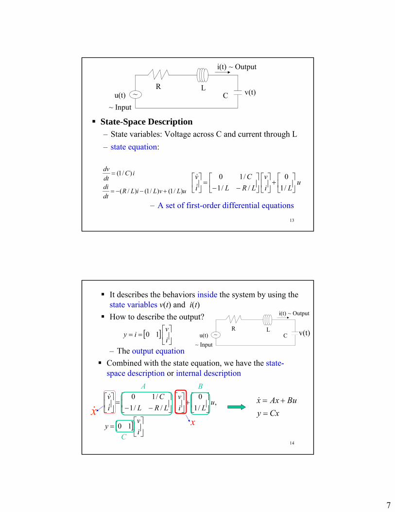
13
~ Output
R L C u(t)
i(t)
~ Input
~
State-Space Description– State variables: Voltage across C and current through L
uLvLiLRdtdi
iCdtdv
)/1()/1()/(
)/1(
+−−=
=
v(t)
– state equation:
– A set of first-order differential equations
uLi
vLRL
Civ
⎥⎦
⎤⎢⎣
⎡+⎥
⎦
⎤⎢⎣
⎡⎥⎦
⎤⎢⎣
⎡−−
=⎥⎦
⎤⎢⎣
⎡/10
//1/10
&
&
14
It describes the behaviors inside the system by using the state variables v(t) and i(t)How to describe the output?
[ ] ⎥⎦
⎤⎢⎣
⎡==
iv
iy 10
– The output equationCombined with the state equation, we have the state-space description or internal description
~ Output
R L C u(t)
i(t)
~ Input
~ v(t)
[ ] ⎥⎦
⎤⎢⎣
⎡=
⎥⎦
⎤⎢⎣
⎡+⎥
⎦
⎤⎢⎣
⎡⎥⎦
⎤⎢⎣
⎡−−
=⎥⎦
⎤⎢⎣
⎡
iv
y
uLi
vLRL
Civ
10
,/10
//1/10
&
&
CxyBuAxx
=+=&
x
A B
C
x&

8
15
A general form:
⎥⎥⎥⎥⎥
⎦
⎤
⎢⎢⎢⎢⎢
⎣
⎡
=
⎥⎥⎥⎥⎥
⎦
⎤
⎢⎢⎢⎢⎢
⎣
⎡
=
⎥⎥⎥⎥
⎦
⎤
⎢⎢⎢⎢
⎣
⎡
=⎩⎨⎧
==
qpn y
yy
y
u
uu
u
x
xx
xtuxhytuxfx
MMM
& 2
1
2
1
2
1
,,,),,(),,(
Main features of the state-space approach It describes the behaviors inside the system Characterizes stability and performances without solving
the differential equations Applicable to more general systems, nonlinear,
time-varying, uncertain, hybrid Most recent advancements in control theory are developed
via a state-space approach
16
Textbook:– Chi-Tsong Chen, Linear System Theory and Design,
3rd Edition, Oxford University Press, 1999 (Required)Reference: – Peter B. Luh, Introduction to Systems Theory,
Lecture note, University of Connecticut, Fall 2004
1.2 Course Overview

9
17
Goals: To achieve a thorough understanding about systems theory and multivariable system design Tentative Outline (13 lectures):– Introduction – Modeling: Use diff. equ. to describe a physical system – The fundamentals of linear algebra– Analysis:
• Quantitative: How to derive response for a given input • Qualitative: How to analyze controllability,
observability, stability and robustness without knowing the exact solution?
18
– Design: • How to realize a system given its mathematical
description • How to design a control law so that desired
output response is produced• How to design an observer to estimate the state
of the system • How to design optimal control laws
– Continuous-time and discrete-time systems will be treated in parallel

10
19
Prerequisites:– 16:413 Linear Feedback Systems– Background on
• Linear algebra: Matrices, vectors, determinant,eigenvalue, solving a system of equations
• z-transform• Ordinary differential equations• Laplace transform, and • Modeling of electrical and mechanical systems
20
• Grading:Homework 20%Mid Term 30%Project 20%Final Examination 30%
All exams are open book, open notes

11
21
• General Rules:– Homework should be clear, concise, and complete– Discussion is allowed but no copying. Make sure
you understand what you write down.– Homework due next class. Strong reasons needed
for late homework– Homework solutions will be provided a week after the
due date at class website• Attendance: will be taken occasionally. Positive
attitude is a key to success.
• If you decide to do something, use your heart and do it well. Otherwise it will be a waste of time.
22
Course Project
Mu
θ
y
A cart with an inverted pendulum (page 22, Chen’s book)
u: control input, external force (Newton)y: displacement of the cart (meter)θ: angle of the pendulum (radiant)
The control problems are1: Stabilization: bring the pendulum to the inverted position and keep it there.
Assume the angle is initially small enough. 2: Assume the pendulum is initially downward. Design a control algorithm to
bring it upward and keep inverted.Assume that there is no friction or damping. The nonlinear model is as follows.
⎥⎦
⎤⎢⎣
⎡ −=⎥
⎦
⎤⎢⎣
⎡⎥⎦
⎤⎢⎣
⎡ +
θgθθmlu
θy
lθθmlmM
sinsin
coscos 2&
&&&&
m
9.8g cart, theof mass :5pendulum theoflength :2.0
pendulum theof mass :1
====
kgMml
kgm

12
23
1. Derive a linear model for the system.2. Design feedback laws using Matlab.3. Validate your designs with Simulink and animation.
Problems:
24
A magnetic suspension system
Purpose: used as an assist device to increase the blood flow rateso as to maintain necessary activities
• How it works: the rotor rotates at certain speed to produce therequired pressure increase and flow rate (e.g., 2L/min)
• Feature: the rotor is magnetically suspended. There is no contactwith the housing.
• Advantage: Minimal damage to blood cells, free flow path, can be used for a longer time than mechanically suspended pump.
• The tricky part: the magnetic suspension. It has to be achieved with high precision feedback control
The clearance< 0.2mm

13
25
Control design plays the most important role in suspension
Active magnetic bearing,desired force generated via controlling the coil currents
Passive magnetic bearings (permanent magnets)help to stabilize the rotor.
• Control objective: Keep the rotor from touching the housing in the presence of flow disturbances and gravity
• Feedback control: the gap at different locations are determined by sensors.The control algorithm use this detected information to figure out the active magnetic force and coil current. The power amplifier produce the requiredcurrents.
• What are in the loop? Position sensor, AD converter, DSP, DA converter,power amplifier.
The clearance< 0.2mm
26
What are in the loop? Position sensor, AD converter, DSP, DA converter,power amplifier.
ADDSPDA
Power amplifiersPosition sensors
Control algorithmImplementation
Advanced design method is needed

14
27
A magnetic suspension test rig (Ball Hall 406)
This experiment is part of the NSF project: (Sept. 06 – Aug. 09). The control objective is to keep the free end of the beam suspended. The gap between the beam and the electromagnet follows any set value via a nonlinear controller, which is implemented by a microprocessor,or the Labview. An eddie-current sensor converts the gap into a voltage signal which is fed into the microprocessor; The controller in the microprocessor computes the desired currents and output it to a power amplifier.
28
The beam rests on the stator when the controller is turned off
The beam suspended when a nonlinear feedback control is applied.

15
29
The robust controller adjusts the current of the electromagnet so that the gap is maintained at the same set value under different load
30
2. Mathematical Descriptions of Systems(Review)
– Classification of systems– Linear systems– Linear time invariant (LTI) systems
⎥⎥⎥⎥⎥
⎦
⎤
⎢⎢⎢⎢⎢
⎣
⎡
=
⎥⎥⎥⎥⎥
⎦
⎤
⎢⎢⎢⎢⎢
⎣
⎡
=
)(
)()(
)(,
)(
)()(
)( 2
1
2
1
ty
tyty
ty
tu
tutu
tu
qp
MM
System)(tu )(ty
)(ku )(ky

16
31
Basic assumption: When an input signal is applied to the system, a unique output is obtained
Q. How do we classify systems?– Number of inputs/outputs; with/without memory;
causality; dimensionality; linearity; time invarianceThe number of inputs and outputs– When p = q = 1, it is called a single-input single-
output (SISO) system– When p > 1 and q > 1, it is called a multi-input
multi-output (MIMO) system– MISO, SIMO defined similarly
2.1 Classification of Systems
32
• Memoryless vs. with Memory– If y(t) depends on u(t) only, the system is said to be
memoryless, otherwise, it has memory– An example of a memoryless system?
+ -
u(t) R1 R2
+y(t)-
A purely resistive circuit
)t(uRR
R)t(y21
2+
= ~ Memoryless
– An example of a system with memory?
+ -
u(t)
R
L
i u
dtdiLRi =+ u
Li
LR
dtdior 1
=+
( ) ( )∫
−−−−+=
t
t
tLRtt
LR
dueL
tieti0
0 )(1)()( 0 τττ

17
33
– i(t) depends on i(t0) and u(τ) for t0 ≤ τ ≤ t, not just u(t)– A system with memory
• Causality: No output before an input is applied Input
SystemOutput
– A system is causal or non-anticipatory if y(t0) depends only on u(t) for t ≤ t0 and is independent of u(t) for t > t0
– Is the circuit discussed last time causal?
+ -
u(t)
R
L
i
t u(t)
1
t y(t)
1
34
– An example of a non-causal system?– y(t) = u(t + 2)
tu(t)
1
t
y(t)1
– Can you truly build a physical system like this? – All physical systems are causal!

18
35
The Concept of State– The state of a system at t0 is the information at t0
that, together with u[t0,∞), uniquely determines the behavior of the system for t ≥ t0
– The number of state variables = the number of ICs needed to solve the problem
– For an RLC circuit, the number of state variables = the number of C + the number of L (except for degenerated cases)
– A natural way to choose state variables as what we have done earlier: {vc} and {iL}
– Is this the unique way to choose state variables?
36
– Any invertible transformation of the above can serve as a state, e.g.,
⎥⎦
⎤⎢⎣
⎡ +=⎥
⎦
⎤⎢⎣
⎡⎥⎦
⎤⎢⎣
⎡=⎥
⎦
⎤⎢⎣
⎡)(
)()(2)()(
1012
)()(
2
1
tititv
titv
txtx
– Although the number of state variables = 2, there are infinite numbers of representations
Order of dimension of a system: The number of state variables– If the dimension is a finite number ⇒ Finite
dimensional (or lumped) system– Otherwise, an infinite dimensional (or distributed)
system

19
37
An example of an infinite dimensional system u(t)
Systemy(t) = u(t-1) A delay line
tu(t)
ty(t)
1
– Given u(t) for t ≥ 0, what information is needed to know y(t) for t ≥ 0?
?
?
– We need an infinite amount of information ⇒ An infinite dimensional system
38
Today:– Introduction
• Motivation• Course Overview
– Mathematical Descriptions of Systems ~ Review• Classification of Systems• Linear Systems• LTI Systems
20
39
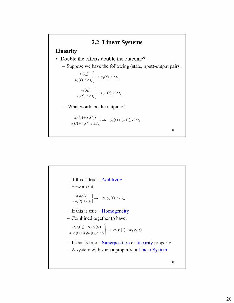
2.2 Linear SystemsLinearity• Double the efforts double the outcome?
– Suppose we have the following (state,input)-output pairs:
0101
01 ),(),(
)(ttty
tttutx
≥→⎭⎬⎫
≥
0202
02 ),(),(
)(ttty
tttutx
≥→⎭⎬⎫
≥
→⎭⎬⎫
≥++
021
0201
),()()()(tttutu
txtx
– What would be the output of
021 ),()( tttyty ≥+
40
– If this is true ~ Additivity– How about
→⎭⎬⎫
≥ 01
01
),()(
tttutx
αα
01 ),( ttty ≥α
→⎭⎬⎫
≥++
02211
022011
),()()()(tttutu
txtxαα
αα
– If this is true ~ Homogeneity– Combined together to have:
)()( 2211 tyty αα +
– If this is true ~ Superposition or linearity property– A system with such a property: a Linear System

21
41
• Also, KVL and KCL are linear constraints. When put together, we have a linear system
• Are R, L, and C linear elements?
dtdvCi,
dtdiLv,Riv C
CL
LRR ===
– Yes (differentiation is a linear operation)
i
v
v = Ri
i
v Linear
Affine Nonlinear
42
Linear System
u(t) y(t)
• The additivity property implies that
– Response = zero-input response + zero-state response
⎩⎨⎧
≥ 01
01
),()(
todue)(tttu
txty
⎩⎨⎧
≥=
+⎩⎨⎧
≡=
01
01
1
01
),(0)(
todue)(0)(
)(todue)(
tttutx
tytu
txty
Response of a Linear System
How can we determine the output y(t)?Can be derived from u(t) + the unit impulse response based on linearity

22
43
Let δΔ(t-τ) be a square pulse at time τ with width Δand height 1/Δ
δΔ(t-τ)
τ+Δτt
1/Δ Area = 1
As Δ →0, we obtain a shifted unit impulse
δ(t −τ)
τ
∫∞
∞−
= τττ dutgty )(),()(
Let the unit impulse response be g ( t,τ ). Based on linearity,
44
If the system is causal,
ττ <= ttg for0),( ∫∞−
=t
dutgty τττ )(),()(
A system is said to be relaxed at t0 if the initial state at t0 is 0– In this case, y(t) for t ≥ t0 is caused exclusively by
u(t) for t ≥ t0
∫=t
t
dutgty0
)(),()( τττ

23
45
∫=t
t
dutGty0
)(),()( τττ
gij(t,τ): The impulse response between the jth input and ith output
⎥⎥⎥⎥⎥
⎦
⎤
⎢⎢⎢⎢⎢
⎣
⎡
=
),(),(),(
),(),(),(),(),(),(
),(
21
22221
11211
τττ
ττττττ
τ
tgtgtg
tgtgtgtgtgtg
tG
qpqq
p
p
• How about a system with p inputs and q outputs?– Have to analyze the relationship for input/output pairs
State-Space Description• A linear system can be described by
)()()()()()()()()()(tutDtxtCtytutBtxtAtx
+=+=&
46
2.3 Linear Time-Invariant (LTI) SystemsTime Invariance: The characteristics of a system do not change over time– What are some of the LTI examples? Time-varying
examples?– What happens for an LTI system if u(t) is delayed by T?
t u(t) y(t)
t
u(t-T) y(t-T)
If the same IC is also shifted by T, then

24
47
– This property can be stated as:
}00
(0) ( ),( ), 0x x y t t tu t t
= → ≥≥
}0( ) ( ),( ),x T x y t T t Tu t T t T
= → − ≥− ≥
48
What happens to the unit impulse response when the system is LTI?
∫ −=t
tdtug
0
)()( τττ
∫=t
tdutgty
0
)(),()( τττ
TTTtgtg anyfor),(),( ++= ττ)()0,(),(),( ττττττ −=−=−−= tgtgtgtg
– Only the difference between t and τ matters– What happens to y(t)?
∫ −=t
tdutg
0
)()( τττ
~ Convolution integral)(*)( tutg=
)(ˆ)(ˆ)(ˆ susgsy =

25
49
∫∞
−≡0
)()(ˆ dtetysy st
∫ ∫∞
=
−∞
=⎟⎟⎠
⎞⎜⎜⎝
⎛−=
0 0
)()(t
stdtedutgτ
τττ
∫ ∫∞
=
−−−∞
=⎟⎟⎠
⎞⎜⎜⎝
⎛−=
0
)(
0
)()(t
sts dteedutg ττ
τ
τττ
)(ˆ)(ˆ)(ˆ susgsy =Proof of
)Let (
,)()(0 0
)(
τυ
ττττ
ττ
−=
⎟⎟⎠
⎞⎜⎜⎝
⎛−= ∫ ∫
∞
=
−∞
=
−−
t
deudtetg s
t
ts
50
)0for 0)( Note(
,)()()(ˆ0
<=
⎟⎟⎠
⎞⎜⎜⎝
⎛= ∫ ∫
∞
=
−∞
−=
−
υυ
ττυυτ
τ
τυ
υ
g
deudegsy ss
∫ ∫∞
=
−∞
=
−
⎟⎟⎠
⎞⎜⎜⎝
⎛=
0 0
)()(τ
τ
υ
υ ττυυ deudeg ss
⎟⎟⎠
⎞⎜⎜⎝
⎛⎟⎟⎠
⎞⎜⎜⎝
⎛= ∫∫
∞
=
−∞
=
−
00
)()(τ
τ
υ
υ ττυυ deudeg ss
)(ˆ)(ˆ)(ˆ susgsy ⋅=

26
51
• ~ Transfer function, the Laplace transform of the unit impulse response
)s(g
)(ˆ)(ˆ)(ˆ susGsy ⋅=
⎥⎥⎥⎥⎥
⎦
⎤
⎢⎢⎢⎢⎢
⎣
⎡
=
)(ˆ)(ˆ)(ˆ
)(ˆ)(ˆ)(ˆ)(ˆ)(ˆ)(ˆ
)(ˆ
21
22221
11211
sgsgsg
sgsgsgsgsgsg
sG
qpqq
p
p ~ Transfer-function matrix, or transfer matrix
Transfer-Function Matrix
)(ˆ)(ˆ)(ˆ susgsy ⋅=For SISO system,
For MIMO system,
52
Today:– Introduction
• Motivation• Course Overview
– Mathematical Descriptions of Systems ~ Review• Classification of Systems• Linear Systems• LTI Systems
Next Time: – Linearization; Examples; Discrete-time systems– Linear Algebra
• Basis, representation, and orthonormalization
27
53
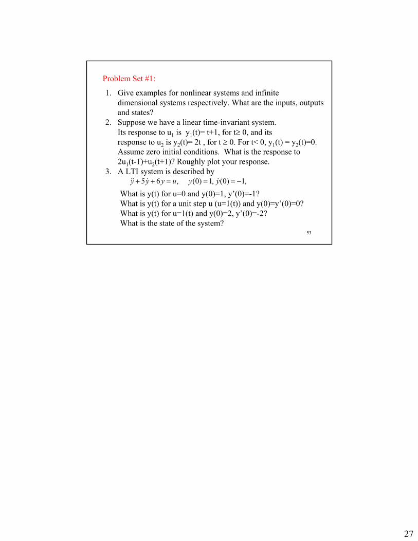
Problem Set #1:
1. Give examples for nonlinear systems and infinite dimensional systems respectively. What are the inputs, outputsand states?
2. Suppose we have a linear time-invariant system. Its response to u1 is y1(t)= t+1, for t≥ 0, and its response to u2 is y2(t)= 2t , for t ≥ 0. For t< 0, y1(t) = y2(t)=0. Assume zero initial conditions. What is the response to2u1(t-1)+u2(t+1)? Roughly plot your response.
3. A LTI system is described by
What is y(t) for u=0 and y(0)=1, y’(0)=-1? What is y(t) for a unit step u (u=1(t)) and y(0)=y’(0)=0?What is y(t) for u=1(t) and y(0)=2, y’(0)=-2?What is the state of the system?
,1)0(,1)0(,65 −===++ yyuyyy &&&&