Embed Size (px)
Citation preview
16.410/413Principles of Autonomy and Decision Making
Lecture 15: Sampling-Based Algorithms for Motion Planning
Emilio Frazzoli
Aeronautics and AstronauticsMassachusetts Institute of Technology
November 3, 2010
Reading: LaValle, Ch. 5S. Karaman and E. Frazzoli, 2011
E. Frazzoli (MIT) L15: Sampling-Based Motion Planning November 3, 2010 1 / 30

The Motion Planning problem
Get from point A to point B avoiding obstacles
E. Frazzoli (MIT) L15: Sampling-Based Motion Planning November 3, 2010 2 / 30

The Motion Planning problem
Consider a dynamical control system defined by an ODE of the form
dx/dt = f (x , u), x(0) = xinit, (1)
where x is the state, u is the control.
Given an obstacle set Xobs ⊂ Rd , and a goal set Xgoal ⊂ Rd , the objective of themotion planning problem is to find, if it exists, a control signal u such that thesolution of (1) satisfies x(t) /∈ Xobs for all t ∈ R+, and x(t) ∈ Xgoal for all t > T ,for some finite T ≥ 0. Return failure if no such control signal exists.
Basic problem in robotics (and intelligent life in general).
Provably very hard: a basic version (the Generalized Piano Mover’s problem)is known to be PSPACE-hard [Reif, ’79].
E. Frazzoli (MIT) L15: Sampling-Based Motion Planning November 3, 2010 2 / 30

Mobility, Brains, and the lack thereof
The Sea Squirt, or Tunicate, is an organism capable of mobility until it finds asuitable rock to cement itself in place. Once it becomes stationary, it digests itsown cerebral ganglion, or “eats its own brain” and develops a thick covering, a
“tunic” for self defense. [S. Soatto, 2010, R. Bajcsy, 1988]
E. Frazzoli (MIT) L15: Sampling-Based Motion Planning November 3, 2010 3 / 30
Image of sea squirts removed due to copyright restrictions. Please see: http://en.wikipedia.org/wiki/File:Sea-tulip.jpg.
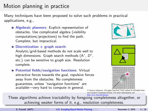
Motion planning in practice
Many techniques have been proposed to solve such problems in practicalapplications, e.g.,
Algebraic planners: Explicit representation ofobstacles. Use complicated algebra (visibilitycomputations/projections) to find the path.Complete, but impractical.
Discretization + graph search:Analytic/grid-based methods do not scale well tohigh dimensions. Graph search methods (A∗, D∗,etc.) can be sensitive to graph size. Resolutioncomplete.
Potential fields/navigation functions: Virtualattractive forces towards the goal, repulsive forcesaway from the obstacles. No completenessguarantees, unless “navigation functions” areavailable—very hard to compute in general.
These algorithms achieve tractability by foregoing completeness altogether, orachieving weaker forms of it, e.g., resolution completeness.
E. Frazzoli (MIT) L15: Sampling-Based Motion Planning November 3, 2010 4 / 30
© Source unknown. All rights reserved. This content is excluded fromour Creative Commons license. For more information, seehttp://ocw.mit.edu/fairuse.
Sampling-based algorithms
A recently proposed class of motion planning algorithms that has been verysuccessful in practice is based on (batch or incremental) sampling methods:solutions are computed based on samples drawn from some distribution.Sampling algorithms retain some form of completeness, e.g., probabilistic orresolution completeness.
Incremental sampling methods are particularly attractive:
Incremental-sampling algorithms lend themselves easily to real-time, on-lineimplementation.
Applicable to very general dynamical systems.
Do not require the explicit enumeration of constraints.
Adaptively multi-resolution methods(i.e., make your own grid as you go along, up to the necessary resolution).
E. Frazzoli (MIT) L15: Sampling-Based Motion Planning November 3, 2010 5 / 30

Probabilistic RoadMaps (PRM)
Introduced by Kavraki and Latombe in 1994.
Mainly geared towards “multi-query” motion planning problems.
Idea: build (offline) a graph (i.e., the roadmap) representing the“connectivity” of the environment; use this roadmap to figure out pathsquickly at run time.
Learning/pre-processing phase:1 Sample n points from Xfree = [0, 1]d \ Xobs.2 Try to connect these points using a fast “local planner” (e.g., ignore
obstacles).3 If connection is successful (i.e., no collisions), add an edge between the points.
At run time:1 Connect the start and end goal to the closest nodes in the roadmap.2 Find a path on the roadmap.
First planner ever to demonstrate the ability tosolve general planning problems in > 4-5 dimensions!
E. Frazzoli (MIT) L15: Sampling-Based Motion Planning November 3, 2010 6 / 30

Probabilistic RoadMap example
238 S. M. LaValle: Planning Algorithms
BUILD ROADMAP1 G.init(); i ! 0;2 while i < N3 if !(i) " Cfree then4 G.add vertex(!(i)); i ! i + 1;5 for each q " neighborhood(!(i),G)6 if ((not G.same component(!(i), q)) and connect(!(i), q)) then7 G.add edge(!(i), q);
Figure 5.25: The basic construction algorithm for sampling-based roadmaps. Notethat i is not incremented if !(i) is in collision. This forces i to correctly count thenumber of vertices in the roadmap.
!(i)
Cobs
Cobs
Figure 5.26: The sampling-based roadmap is constructed incrementally by at-tempting to connect each new sample, !(i), to nearby vertices in the roadmap.
Generic preprocessing phase Figure 5.25 presents an outline of the basicpreprocessing phase, and Figure 5.26 illustrates the algorithm. As seen throughoutthis chapter, the algorithm utilizes a uniform, dense sequence !. In each iteration,the algorithm must check whether !(i) " Cfree. If !(i) " Cobs, then it mustcontinue to iterate until a collision-free sample is obtained. Once !(i) " Cfree,then in line 4 it is inserted as a vertex of G. The next step is to try to connect !(i)to some nearby vertices, q, of G. Each connection is attempted by the connectfunction, which is a typical LPM (local planning method) from Section 5.4.1.In most implementations, this simply tests the shortest path between !(i) andq. Experimentally, it seems most e!cient to use the multi-resolution, van derCorput–based method described at the end of Section 5.3.4 [379]. Instead of theshortest path, it is possible to use more sophisticated connection methods, suchas the bidirectional algorithm in Figure 5.24. If the path is collision-free, thenconnect returns true.
The same component condition in line 6 checks to make sure !(i) and q arein di"erent components of G before wasting time on collision checking. This en-sures that every time a connection is made, the number of connected components
“Practical” algorithm:Incremental constructionConnect points within a radius r , starting from “closest” ones.Do not attempt to connect points that are already on the same connectedcomponent of the PRM.
What kind of properties does this algorithm have? Will it find a solution if there isone? Is this an optimal solution? What is the complexity of the algorithm?
E. Frazzoli (MIT) L15: Sampling-Based Motion Planning November 3, 2010 7 / 30

Probabilistic Completeness
Definition (Probabilistic completeness)
An algorithm ALG is probabilistically complete if, for any robustly feasible motionplanning problem defined by P = (Xfree, xinit,Xgoal),
limN→∞
Pr (ALG returns a solution to P) = 1.
A “relaxed” notion of completeness
Applicable to motion planning problems with a robust solution. A robustsolution remains a solution if obstacles are “dilated” by some small δ.
Robust NOT Robust
E. Frazzoli (MIT) L15: Sampling-Based Motion Planning November 3, 2010 8 / 30

Asymptotic Optimality
Definition (Asymptotic optimality)
An algorithm ALG is asymptotically optimal if, for any motion planning problemP = (Xfree, xinit,Xgoal) and cost function c that admit a robust optimal solutionwith finite cost c∗,
P(
limi→∞
Y ALGi = c∗
)= 1.
The function c associates to each path σ a non-negative cost c(σ), e.g.,c(σ) =
∫σχ(s) ds.
The definition is applicable to optimal motion planning problem with arobust optimal solution. A robust optimal solution is such that it can beobtained as a limit of robust (non-optimal) solutions.
Not robust Robust
E. Frazzoli (MIT) L15: Sampling-Based Motion Planning November 3, 2010 9 / 30

Complexity
How can we measure complexity for an algorithm that does not necessarilyterminate?
Treat the number of samples as “the size of the input.” (Everything elsestays the same)
Also, complexity per sample: how much work (time/memory) is needed toprocess one sample.
Useful for comparison of sampling-based algorithms.
Cannot compare with deterministic, complete algorithms.
E. Frazzoli (MIT) L15: Sampling-Based Motion Planning November 3, 2010 10 / 30

Simple PRM (sPRM)
sPRM Algorithm
V ← xinit ∪ SampleFreeii=1,...,N−1; E ← ∅;foreach v ∈ V do
U ← Near(G = (V ,E ), v , r) \ v;foreach u ∈ U do
if CollisionFree(v , u) then E ← E ∪ (v , u), (u, v)return G = (V ,E );
The simplified version of the PRM algorithm has been shown to beprobabilistically complete. (No proofs available for the “real” PRM!)
Moreover, the probability of success goes to 1 exponentially fast, if theenvironment satisfies certain “good visibility” conditions.
New key concept: combinatorial complexity vs. “visibility”
E. Frazzoli (MIT) L15: Sampling-Based Motion Planning November 3, 2010 11 / 30

Remarks on PRM
sPRM is probabilistically complete and asymptotically optimal.
PRM is probabilistically complete but NOT asymptotically optimal.
Complexity for N samples: Θ(N2).
Practical complexity-reduction tricks:
k-nearest neighbors: connect to the k nearest neighbors. ComplexityΘ(N logN). (Finding nearest neighbors takes logN time.)
Bounded degree: connect at most k neighbors among those within radius r .
Variable radius: change the connection radius r as a function of N. How?
E. Frazzoli (MIT) L15: Sampling-Based Motion Planning November 3, 2010 12 / 30

Rapidly-exploring Random Trees
Introduced by LaValle and Kuffner in 1998.
Appropriate for single-query planning problems.
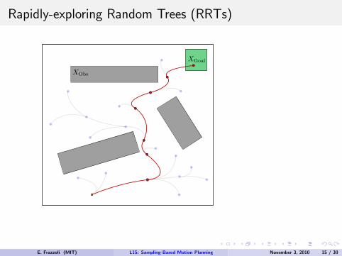
Idea: build (online) a tree, exploring the region of the state space that can bereached from the initial condition.
At each step: sample one point from Xfree, and try to connect it to theclosest vertex in the tree.
Very effective in practice, “Voronoi bias”
E. Frazzoli (MIT) L15: Sampling-Based Motion Planning November 3, 2010 13 / 30
Rapidly-exploring Random Trees
RRT
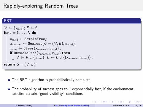
V ← xinit; E ← ∅;for i = 1, . . . ,N do
xrand ← SampleFreei ;xnearest ← Nearest(G = (V ,E ), xrand);xnew ← Steer(xnearest, xrand) ;if ObtacleFree(xnearest, xnew) then
V ← V ∪ xnew; E ← E ∪ (xnearest, xnew) ;
return G = (V ,E );
The RRT algorithm is probabilistically complete.
The probability of success goes to 1 exponentially fast, if the environmentsatisfies certain “good visibility” conditions.
E. Frazzoli (MIT) L15: Sampling-Based Motion Planning November 3, 2010 14 / 30

Rapidly-exploring Random Trees (RRTs)
E. Frazzoli (MIT) L15: Sampling-Based Motion Planning November 3, 2010 15 / 30
Rapidly-exploring Random Trees (RRTs)
E. Frazzoli (MIT) L15: Sampling-Based Motion Planning November 3, 2010 15 / 30

Rapidly-exploring Random Trees (RRTs)
E. Frazzoli (MIT) L15: Sampling-Based Motion Planning November 3, 2010 15 / 30

Rapidly-exploring Random Trees (RRTs)
E. Frazzoli (MIT) L15: Sampling-Based Motion Planning November 3, 2010 15 / 30

Rapidly-exploring Random Trees (RRTs)
E. Frazzoli (MIT) L15: Sampling-Based Motion Planning November 3, 2010 15 / 30

Rapidly-exploring Random Trees (RRTs)
E. Frazzoli (MIT) L15: Sampling-Based Motion Planning November 3, 2010 15 / 30

Rapidly-exploring Random Trees (RRTs)
E. Frazzoli (MIT) L15: Sampling-Based Motion Planning November 3, 2010 15 / 30

Rapidly-exploring Random Trees (RRTs)
E. Frazzoli (MIT) L15: Sampling-Based Motion Planning November 3, 2010 15 / 30

Rapidly-exploring Random Trees (RRTs)
E. Frazzoli (MIT) L15: Sampling-Based Motion Planning November 3, 2010 15 / 30

Rapidly-exploring Random Trees (RRTs)
E. Frazzoli (MIT) L15: Sampling-Based Motion Planning November 3, 2010 15 / 30

Rapidly-exploring Random Trees (RRTs)
E. Frazzoli (MIT) L15: Sampling-Based Motion Planning November 3, 2010 15 / 30

Rapidly-exploring Random Trees (RRTs)
E. Frazzoli (MIT) L15: Sampling-Based Motion Planning November 3, 2010 15 / 30

Rapidly-exploring Random Trees (RRTs)
E. Frazzoli (MIT) L15: Sampling-Based Motion Planning November 3, 2010 15 / 30
Rapidly-exploring Random Trees (RRTs)
E. Frazzoli (MIT) L15: Sampling-Based Motion Planning November 3, 2010 15 / 30

Rapidly-exploring Random Trees (RRTs)
E. Frazzoli (MIT) L15: Sampling-Based Motion Planning November 3, 2010 15 / 30

Rapidly-exploring Random Trees (RRTs)
E. Frazzoli (MIT) L15: Sampling-Based Motion Planning November 3, 2010 15 / 30

Rapidly-exploring Random Trees (RRTs)
E. Frazzoli (MIT) L15: Sampling-Based Motion Planning November 3, 2010 15 / 30

Rapidly-exploring Random Trees (RRTs)
E. Frazzoli (MIT) L15: Sampling-Based Motion Planning November 3, 2010 15 / 30

Rapidly-exploring Random Trees (RRTs)
E. Frazzoli (MIT) L15: Sampling-Based Motion Planning November 3, 2010 15 / 30
Rapidly-exploring Random Trees (RRTs)
E. Frazzoli (MIT) L15: Sampling-Based Motion Planning November 3, 2010 15 / 30

Voronoi bias
Definition (Voronoi diagram)
Given n sites in d dimensions, the Voronoi diagram of the sites is a partition of Rd
into regions, one region per site, such that all points in the interior of each regionlie closer to that regions site than to any other site.
Vertices of the RRT that are more “isolated” (e.g., in unexplored areas, or atthe boundary of the explored area) have larger Voronoi regions—and aremore likely to be selected for extension.
E. Frazzoli (MIT) L15: Sampling-Based Motion Planning November 3, 2010 16 / 30
© Source unknown. All rights reserved. This content is excluded from our CreativeCommons license. For more information, see http://ocw.mit.edu/fairuse.
Image by MIT OpenCourseWare.
RRTs in action
Talos, the MIT entry to the 2007 DARPA Urban Challenge, relied on an“RRT-like” algorithm for real-time motion planning and control.
The devil is in the details: provisions needed for, e.g.,
Real-time, on-line planning for a safety-critical vehicle with substantialmomentum.Uncertain, dynamic environment with limited/faulty sensors.
Main innovations [Kuwata, et al. ’09]
Closed-loop planning: plan reference trajectories for an closed-loop model ofthe vehicle under a stabilizing feedback.
Safety invariance: Always maintain the ability to stop safely within thesensing region.
Lazy evaluation: the actual trajectory may deviate from the planned one,need to efficiently re-check the tree for feasibility.
The RRT-based P+C system performed flawlessly throughout the race.
E. Frazzoli (MIT) L15: Sampling-Based Motion Planning November 3, 2010 17 / 30
Limitations of current incremental sampling methods
The MIT DARPA Urban Challenge code, as well as other incremental samplingmethods, suffer from the following limitations:
No characterization of the quality (e.g., “cost”) of the trajectories returnedby the algorithm.
Keep running the RRT even after the first solution has been obtained, for aslong as possible (given the real-time constraints), hoping to find a betterpath than that already available.
No systematic method for imposing temporal/logical constraints, such as,e.g., the rules of the road, complicated mission objectives, ethical/deonticcode.
In the DARPA Urban Challenge, all logics for, e.g., intersection handling, hadto be hand-coded, at a huge cost in terms of debugging effort/reliability ofthe code.
E. Frazzoli (MIT) L15: Sampling-Based Motion Planning November 3, 2010 18 / 30

RRTs and optimality
RRTs are great at finding feasible trajectories quickly...
However, RRTs are apparently terrible at finding good trajectories.
What is the reason for such behavior?
E. Frazzoli (MIT) L15: Sampling-Based Motion Planning November 3, 2010 19 / 30

A negative result [K&F RSS’10]
Let Y RRTn be the cost of the best path in the RRT at the end of iteration n.
It is easy to show that Y RRTn converges (to a random variable), i.e.,
limn→∞
Y RRTn = Y RRT
∞ .
The random variable Y RRT∞ is sampled from a distribution with zero mass at
the optimum:
Theorem (Almost sure suboptimality of RRTs)
If the set of sampled optimal paths has measure zero, the sampling distribution isabsolutely continuous with positive density in Xfree, and d ≥ 2, then the best pathin the RRT converges to a sub-optimal solution almost surely, i.e.,
Pr[Y RRT∞ > c∗
]= 1.
E. Frazzoli (MIT) L15: Sampling-Based Motion Planning November 3, 2010 20 / 30
Some remarks on the negative result
Intuition: RRT does not satisfy a necessary condition for asymptoticoptimality, i.e., that the root node has infinitely many subtrees that extend atleast a distance ε away from xinit.
The RRT algorithm “traps” itself by disallowing new better paths to emerge.
Heuristics such as
running the RRT multiple times [Ferguson & Stentz, ’06]running multiple trees concurrently,deleting and rebuilding parts of the tree etc.
work better than the standard RRT, but also result in almost-suresub-optimality.
A careful rethinking of the RRT algorithm seems to be required toensure (asymptotic) optimality.
E. Frazzoli (MIT) L15: Sampling-Based Motion Planning November 3, 2010 21 / 30
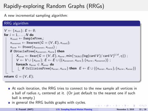
Rapidly-exploring Random Graphs (RRGs)
A new incremental sampling algorithm:
RRG algorithm
V ← xinit; E ← ∅;for i = 1, . . . ,N do
xrand ← SampleFreei ;xnearest ← Nearest(G = (V ,E), xrand);xnew ← Steer(xnearest, xrand) ;if ObtacleFree(xnearest, xnew) then
Xnear ← Near(G = (V ,E), xnew,minγRRG(log(cardV )/ cardV )1/d , η) ;V ← V ∪ xnew; E ← E ∪ (xnearest, xnew), (xnew, xnearest) ;foreach xnear ∈ Xnear do
if CollisionFree(xnear, xnew) then E ← E ∪ (xnear, xnew), (xnew, xnear)
return G = (V ,E);
At each iteration, the RRG tries to connect to the new sample all vertices ina ball of radius rn centered at it. (Or just default to the nearest one if suchball is empty.)in general the RRG builds graphs with cycles.
E. Frazzoli (MIT) L15: Sampling-Based Motion Planning November 3, 2010 22 / 30

Properties of RRGs
Theorem (Probabilistic completeness)
Since V RRGn = V RRT
n , for all n, it follows that RRG has the same completenessproperties as RRT, i.e.,
Pr[V RRGn ∩ Xgoal = ∅
]= O(e−bn).
Theorem (Asymptotic Optimality)
If the Near procedure returns all nodes in V within a ball of volume
Vol = γlog n
n, γ > 2d(1 + 1/d),
under some additional technical assumptions (e.g., on the sampling distribution,on the ε clearance of the optimal path, and on the continuity of the cost function),the best path in the RRG converges to an optimal solution almost surely, i.e.,
Pr[Y RRG∞ = c∗
]= 1.
E. Frazzoli (MIT) L15: Sampling-Based Motion Planning November 3, 2010 23 / 30

Computational Complexity [K&F RSS ’10]
At each iteration, the RRG algorithm executes O(log n) extra calls toObstacleFree when compared to the RRT.
However, the complexity of the Nearest procedure is Ω(log n).Achieved if using, e.g., a Balanced-Box Decomposition (BBD) Tree.
Theorem: Asymptotic (Relative) Complexity
There exists a constant β ∈ R+ such that
lim supi→∞
E[
OPSRRGi
OPSRRTi
]≤ β
In other words, the RRG algorithm has no substantial computationaloverhead over RRT, and ensures asymptotic optimality.
E. Frazzoli (MIT) L15: Sampling-Based Motion Planning November 3, 2010 24 / 30
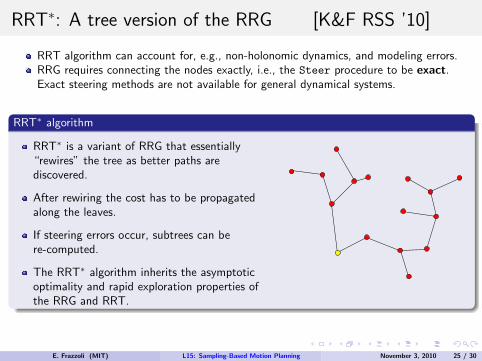
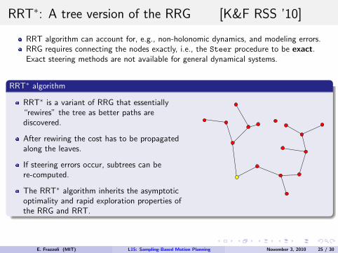
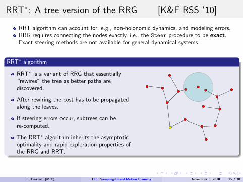
RRT∗: A tree version of the RRG [K&F RSS ’10]
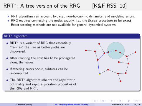
RRT algorithm can account for, e.g., non-holonomic dynamics, and modeling errors.RRG requires connecting the nodes exactly, i.e., the Steer procedure to be exact.Exact steering methods are not available for general dynamical systems.
RRT∗ algorithm
RRT∗ is a variant of RRG that essentially“rewires” the tree as better paths arediscovered.
After rewiring the cost has to be propagatedalong the leaves.
If steering errors occur, subtrees can bere-computed.
The RRT∗ algorithm inherits the asymptoticoptimality and rapid exploration properties ofthe RRG and RRT.
E. Frazzoli (MIT) L15: Sampling-Based Motion Planning November 3, 2010 25 / 30
RRT∗: A tree version of the RRG [K&F RSS ’10]
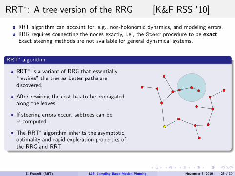
RRT algorithm can account for, e.g., non-holonomic dynamics, and modeling errors.RRG requires connecting the nodes exactly, i.e., the Steer procedure to be exact.Exact steering methods are not available for general dynamical systems.
RRT∗ algorithm
RRT∗ is a variant of RRG that essentially“rewires” the tree as better paths arediscovered.
After rewiring the cost has to be propagatedalong the leaves.
If steering errors occur, subtrees can bere-computed.
The RRT∗ algorithm inherits the asymptoticoptimality and rapid exploration properties ofthe RRG and RRT.
E. Frazzoli (MIT) L15: Sampling-Based Motion Planning November 3, 2010 25 / 30
RRT∗: A tree version of the RRG [K&F RSS ’10]
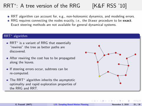
RRT algorithm can account for, e.g., non-holonomic dynamics, and modeling errors.RRG requires connecting the nodes exactly, i.e., the Steer procedure to be exact.Exact steering methods are not available for general dynamical systems.
RRT∗ algorithm
RRT∗ is a variant of RRG that essentially“rewires” the tree as better paths arediscovered.
After rewiring the cost has to be propagatedalong the leaves.
If steering errors occur, subtrees can bere-computed.
The RRT∗ algorithm inherits the asymptoticoptimality and rapid exploration properties ofthe RRG and RRT.
E. Frazzoli (MIT) L15: Sampling-Based Motion Planning November 3, 2010 25 / 30

RRT∗: A tree version of the RRG [K&F RSS ’10]
RRT algorithm can account for, e.g., non-holonomic dynamics, and modeling errors.RRG requires connecting the nodes exactly, i.e., the Steer procedure to be exact.Exact steering methods are not available for general dynamical systems.
RRT∗ algorithm
RRT∗ is a variant of RRG that essentially“rewires” the tree as better paths arediscovered.
After rewiring the cost has to be propagatedalong the leaves.
If steering errors occur, subtrees can bere-computed.
The RRT∗ algorithm inherits the asymptoticoptimality and rapid exploration properties ofthe RRG and RRT.
E. Frazzoli (MIT) L15: Sampling-Based Motion Planning November 3, 2010 25 / 30
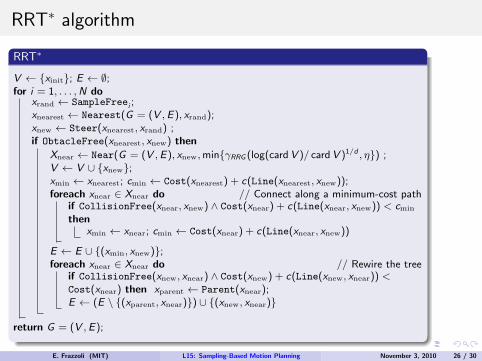
RRT∗ algorithm
RRT∗
V ← xinit; E ← ∅;for i = 1, . . . ,N do
xrand ← SampleFreei ;xnearest ← Nearest(G = (V ,E), xrand);xnew ← Steer(xnearest, xrand) ;if ObtacleFree(xnearest, xnew) then
Xnear ← Near(G = (V ,E), xnew,minγRRG (log(cardV )/ cardV )1/d , η) ;V ← V ∪ xnew;xmin ← xnearest; cmin ← Cost(xnearest) + c(Line(xnearest, xnew));foreach xnear ∈ Xnear do // Connect along a minimum-cost path
if CollisionFree(xnear, xnew) ∧ Cost(xnear) + c(Line(xnear, xnew)) < cmin
thenxmin ← xnear; cmin ← Cost(xnear) + c(Line(xnear, xnew))
E ← E ∪ (xmin, xnew);foreach xnear ∈ Xnear do // Rewire the tree
if CollisionFree(xnew, xnear) ∧ Cost(xnew) + c(Line(xnew, xnear)) <Cost(xnear) then xparent ← Parent(xnear);E ← (E \ (xparent, xnear)) ∪ (xnew, xnear)
return G = (V ,E);
E. Frazzoli (MIT) L15: Sampling-Based Motion Planning November 3, 2010 26 / 30
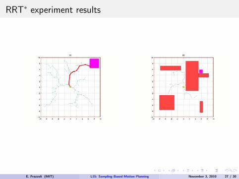
RRT∗ experiment results
E. Frazzoli (MIT) L15: Sampling-Based Motion Planning November 3, 2010 27 / 30
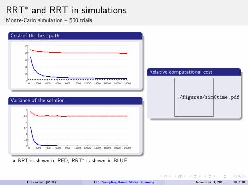
RRT∗ and RRT in simulationsMonte-Carlo simulation – 500 trials
Cost of the best path
0 2000 4000 6000 8000 10000 12000 14000 16000 18000 200009
10
11
12
13
14
Variance of the solution
0 2000 4000 6000 8000 10000 12000 14000 16000 18000 200000
0.5
1
1.5
2
2.5
3
Relative computational cost
./figures/sim0time.pdf
RRT is shown in RED, RRT∗ is shown in BLUE.
E. Frazzoli (MIT) L15: Sampling-Based Motion Planning November 3, 2010 28 / 30

Summary
Key idea in RRG/RRT∗: to combine optimality and computational efficiency,it is necessary to attempt connection to Θ(log N) nodes at each iteration.
Reduce volume of the “connection ball” as log(N)/N;Increase the number of connections as log(N).
These principles can be used to obtain “optimal” versions of PRM, etc.:
Algorithm ProbabilisticCompleteness
AsymptoticOptimality
ComputationalComplexity
sPRM Yes Yes O(N)
k-nearest sPRM No No O(logN)
RRT Yes No O(logN)
PRM∗ Yes Yes O(logN)
k-nearest PRM∗ Yes Yes O(logN)
RRG Yes Yes O(logN)
k-nearest RRG Yes Yes O(logN)
RRT∗ Yes Yes O(logN)
k-nearest RRT∗ Yes Yes O(logN)
E. Frazzoli (MIT) L15: Sampling-Based Motion Planning November 3, 2010 29 / 30
Conclusion
Thorough and rigorous analysis of the optimality properties of incrementalsampling-based motion planning algorithms.
We show that state-of-the-art algorithms such as RRT converge to aNON-optimal solution almost-surely.
We provide new algorithms (RRG and the RRT∗), which almost-surelyconverge to optimal solutions while incurring no significant cost overhead wrtstate-of-the-art-algorithms.
Bibliographical reference: S. Karaman and E. Frazzoli. Sampling-basedalgorithms for optimal motion planning. Int. Journal of Robotics Research,2011. To appear. Also available at http://arxiv.org/abs/1105.1186.
Current Work:
Optimal motion planning with temporal/logic constraints (e.g., µ-calculus).Anytime solution of PDEs (Eikonal equation, Hamilton-Jacobi-Bellman, etc.)Anytime solution of differential gamesStochastic optimal motion planning (process + sensor noise)Multi-agent problems.
E. Frazzoli (MIT) L15: Sampling-Based Motion Planning November 3, 2010 30 / 30

MIT OpenCourseWarehttp://ocw.mit.edu
16.410 / 16.413 Principles of Autonomy and Decision MakingFall 2010
For information about citing these materials or our Terms of Use, visit: http://ocw.mit.edu/terms .