1

151-0917-00 U Stofftransport (Mass Transfer) HS 2019

Exercise 2: Diffusion in Dilute Solutions: Fick’s Laws

1) Chapter 2 Problem 3

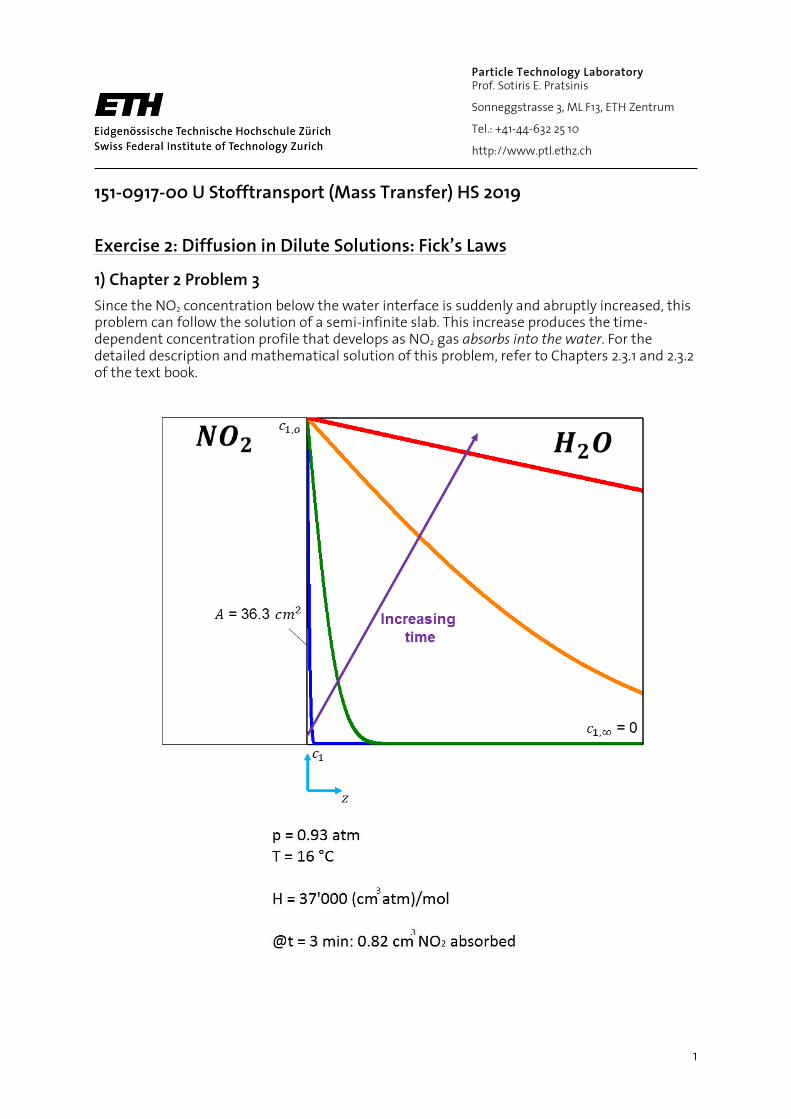
Since the NO2 concentration below the water interface is suddenly and abruptly increased, this problem can follow the solution of a semi-infinite slab. This increase produces the time-dependent concentration profile that develops as NO2 gas absorbs into the water. For the detailed description and mathematical solution of this problem, refer to Chapters 2.3.1 and 2.3.2 of the text book.

Particle Technology Laboratory Prof. Sotiris E. Pratsinis

Sonneggstrasse 3, ML F13, ETH Zentrum

Tel.: +41-44-632 25 10

http://www.ptl.ethz.ch

2

The problem is described by the second Fick’s law:

2

1

2

1

z

cD

t

c

(1)

with following conditions:

t = 0, all z, c1 = c1

t > 0, z = 0, c1 = c10

z = , c1 = c1

Eq. (2.3-18) from the text book can be used for determining the flux across the interface (z = 0).

1 10 10z

Dj c c

t

(2)

From the Henry’s constant and pressure, we can calculate the concentration of NO2 at the interface. c10 = p/H = (0.93 atm)/(37,000 cm3 atm/mol) = 2.5110-5 mol/cm3

The concentration of NO2 far below the surface will be: c1 = 0 The total amount of absorbed NO2 in water can be calculated to integrate (j1z=0 A) from 0 to 180 s like:

180 180180

1 1 10 100 00 0

5 2

3

0.5

12

mol 180s2 2.51 10 36.3cm

cm

mol s0.01339

cm

s ss

z

D DN j Adt c A dt c A t

t

D

D

(3)

The absorbed amount of NO2 also can be calculated from the given change in volume using the ideal gas law:

35 3 6

2 3

1

5

N m0.93atm 1.013 10 0.82cm 10

m atm cm

Nm8.314 273 16 K

mol K

3.22 10 mol

pVN n

RT

(4)

Combining Eq. (4) and Eq. (5), we get

0.55

1

mol s0.01379 3.22 10 mol

cm N D

(5)

Therefore we get finally

D = 5.4810-6 cm2/s.

3

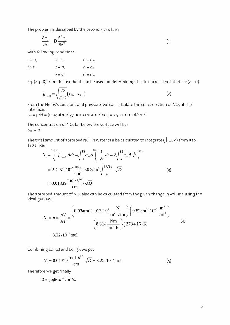
2) Old test problem

a)

b)

This is a semi-infinite slab situation, which can be solved with Fick’s second law.

Boundary conditions:

1 1

1 10

1 1

0 0

0 0 2 /

0 0

t all z c c

t z c c g kg

t z c c

(1)

The solution of Fick’s second law gives:

1 10

10

c cerf

c c

(2)

Calculate the value of erf(z):

0.0015 2

0.99930 2

erf

(3)

From the given table for the error function:

2.40 (4)

with

4

z

Dt

(5)

c

z

c∞

c0 Contaminated waste

Soil

t

z=0

4

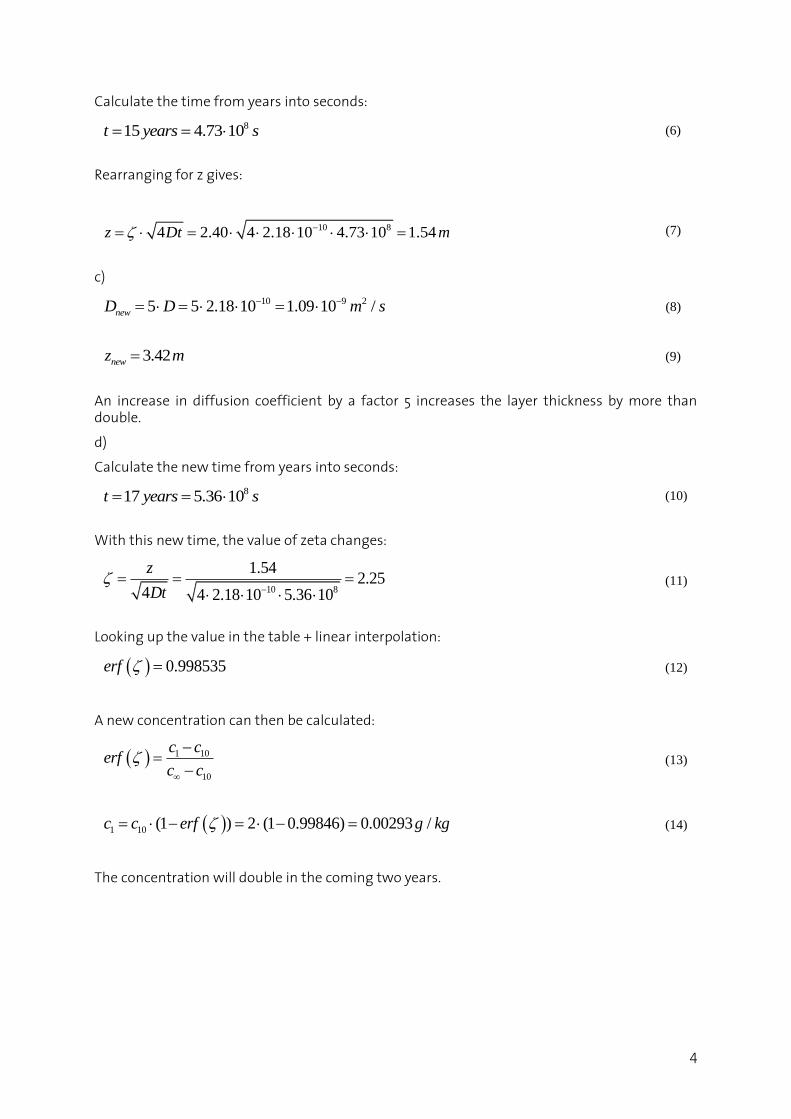
Calculate the time from years into seconds:

815 4.73 10t years s (6)

Rearranging for z gives:

10 84 2.40 4 2.18 10 4.73 10 1.54z Dt m (7)

c)

10 9 25 5 2.18 10 1.09 10 /newD D m s (8)

3.42newz m (9)

An increase in diffusion coefficient by a factor 5 increases the layer thickness by more than double.

d)

Calculate the new time from years into seconds:

817 5.36 10t years s (10)

With this new time, the value of zeta changes:

10 8

1.542.25

4 4 2.18 10 5.36 10

z

Dt

(11)

Looking up the value in the table + linear interpolation:

0.998535erf (12)

A new concentration can then be calculated:

1 10

10

c cerf

c c

(13)

1 10 (1 ) 2 (1 0.99846) 0.00293 /c c erf g kg (14)

The concentration will double in the coming two years.

5

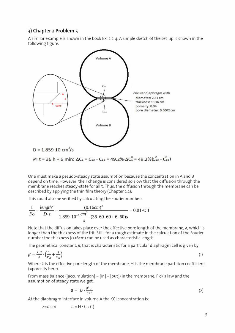
3) Chapter 2 Problem 5

A similar example is shown in the book Ex. 2.2-4. A simple sketch of the set-up is shown in the following figure.

One must make a pseudo-steady state assumption because the concentration in A and B depend on time. However, their change is considered so slow that the diffusion through the membrane reaches steady-state for all t. Thus, the diffusion through the membrane can be described by applying the thin film theory (Chapter 2.2).

This could also be verified by calculating the Fourier number:

2 2

25

1 (0.16 )0.01 1

1.859 10 (36 60 60 6 60)

length cm

cmFo D ts

s

Note that the diffusion takes place over the effective pore length of the membrane, λ, which is longer than the thickness of the frit. Still, for a rough estimate in the calculation of the Fourier number the thickness (0.16cm) can be used as characteristic length.

The geometrical constant, β, that is characteristic for a particular diaphragm cell is given by:

𝛽 =𝐴∙𝐻

𝜆∙ (

1

𝑉𝐴+

1

𝑉𝐵) (1)

Where 𝜆 is the effective pore length of the membrane, H is the membrane partition coefficient (=porosity here).

From mass balance ([accumulation] = [in] – [out]) in the membrane, Fick’s law and the assumption of steady state we get:

0 = 𝐷 ∙𝜕2𝑐1

𝜕𝑧2 (2)

At the diaphragm interface in volume A the KCl concentration is:

z=0 cm c1 = H ∙ C1A (t)

6

And in volume B (z=λ := effective pore length):

z=λ c1 = H ∙ C1B (t)

So when we solve the differential equation (1) :

0 = 𝐷 ∙𝜕2𝑐1

𝜕𝑧2 𝜕𝑐1

𝜕𝑧= 𝑐𝑜𝑛𝑠𝑡. = 𝑎

𝑎 ∙ ∫ 𝜕𝑧 = ∫ 𝜕𝑐1 𝑎 ∙ 𝑧 + 𝑏 = 𝑐1 with a, b = const.

Plug in the boundary conditions and we get:

c1= H ∙ C1A(t) + H ∙ (C1B(t) – C1A(t)) ∙ z/λ

And therefore the flux of KCl at steady state:

𝑗1 = −𝐷 ∙𝜕𝑐1

𝜕𝑧= −

𝐷∙𝐻

𝜆∙ (𝐶1𝐵(𝑡) − 𝐶1𝐴(𝑡))

(3)

Since we are at pseudo-steady state, the concentration in the volumes A and B still change with time and their mass balance gives us time dependent values for C1A and C1B:

𝑉𝐴∙

𝑑𝐶1𝐴(𝑡)

𝑑𝑡= −𝐴 ∙ 𝑗1

11

( ) 1A

A

dC tA j

dt V

11

( ) 1B

B

dC tA j

dt V

𝑉𝐵∙

𝑑𝐶1𝐵(𝑡)

𝑑𝑡= 𝐴 ∙ 𝑗1

By subtracting these two equations, we can get a time-dependent concentration difference:

𝑑

𝑑𝑡(𝐶1𝐴(𝑡) − 𝐶1𝐵(𝑡)) = −𝐴 ∙ 𝑗1 ∙ (

1

𝑉𝐴+

1

𝑉𝐵) (4)

The pseudo-steady state assumption is justified if we have large volumes compared to that of the membrane/diaphragm. A more detailed explanation can be found in Ch. 2-2 on p. 25.

Please make note of the difference in positive/negative sign for the two mass balance equations above. This comes from the fact, that the flux of KCl in A is out of the volume, while for B it is into the volume. The mass balances are simple because the flux j1 from A and the one into B are the same (i.e. no accumulation in the diaphragm).

Combining equations (3) and (4) gives us:

𝑑

𝑑𝑡(𝐶1𝐴(𝑡) − 𝐶1𝐵(𝑡)) = −

𝐴 ∙ 𝐻 ∙ 𝐷

𝜆∙ (

1

𝑉𝐴+

1

𝑉𝐵) ∙ (𝐶1𝐴(𝑡) − 𝐶1𝐵(𝑡)) = −𝛽 ∙ 𝐷 ∙ (𝐶1𝐴(𝑡) − 𝐶1𝐵(𝑡))

Because we know that initially (@ t = 0 s) Volume A has 1 M KCl, while Volume B contains no KCl so:

[𝐶1𝐴 − 𝐶1𝐵]𝑡=0 = 𝐶1𝐴0 − 𝐶1𝐵

0 = 𝐶1𝐴0

So we can solve the differential equation as done in 2.2-4:

𝐶1𝐴(𝑡)−𝐶1𝐵(𝑡)

𝐶1𝐴0 −𝐶1𝐵

0 = 𝑒−𝛽∙𝐷∙𝑡

Or solved for the calibration constant :

𝛽 = 1

𝐷∙𝑡∙ 𝑙𝑛 (

𝐶1𝐴0 −𝐶1𝐵

0

𝐶1𝐴(𝑡)−𝐶1𝐵(𝑡))

By plugging in the numbers for D and the concentration change after 36 h and 6 min (=t) we can calculate the cell calibration constant (a):

7

𝛽 = 1

(1.859 ∙ 10−5)𝑐𝑚2

𝑠∙ (36 ∙ 3600 + 6 ∙ 60)𝑠

∙ 𝑙𝑛 (1

0.492) = 𝟎. 𝟐𝟗𝟒 𝒄𝒎−𝟐

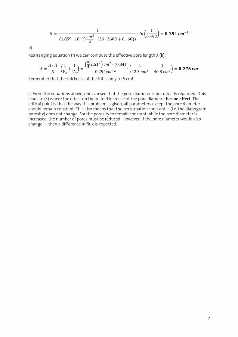
b)

Rearranging equation (1) we can compute the effective pore length λ (b):

𝜆 =𝐴 ∙ 𝐻

𝛽∙ (

1

𝑉𝐴+

1

𝑉𝐵) =

(𝜋4

2.512) 𝑐𝑚2 ∙ (0.34)

0.294𝑐𝑚−2∙ (

1

42.3 𝑐𝑚3+

1

40.8 𝑐𝑚3) = 𝟎. 𝟐𝟕𝟔 𝒄𝒎

Remember that the thickness of the frit is only 0.16 cm!

c) From the equations above, one can see that the pore diameter is not directly regarded . This leads to (c) where the effect on the 10 fold increase of the pore diameter has no effect. The critical point is that the way this problem is given, all parameters except the pore diameter should remain constant. This also means that the perturbation constant H (i.e. the diaphgram porosity) does not change. For the porosity to remain constant while the pore diameter is increased, the number of pores must be reduced! However, if the pore diameter would also change H, then a difference in flux is expected.

8

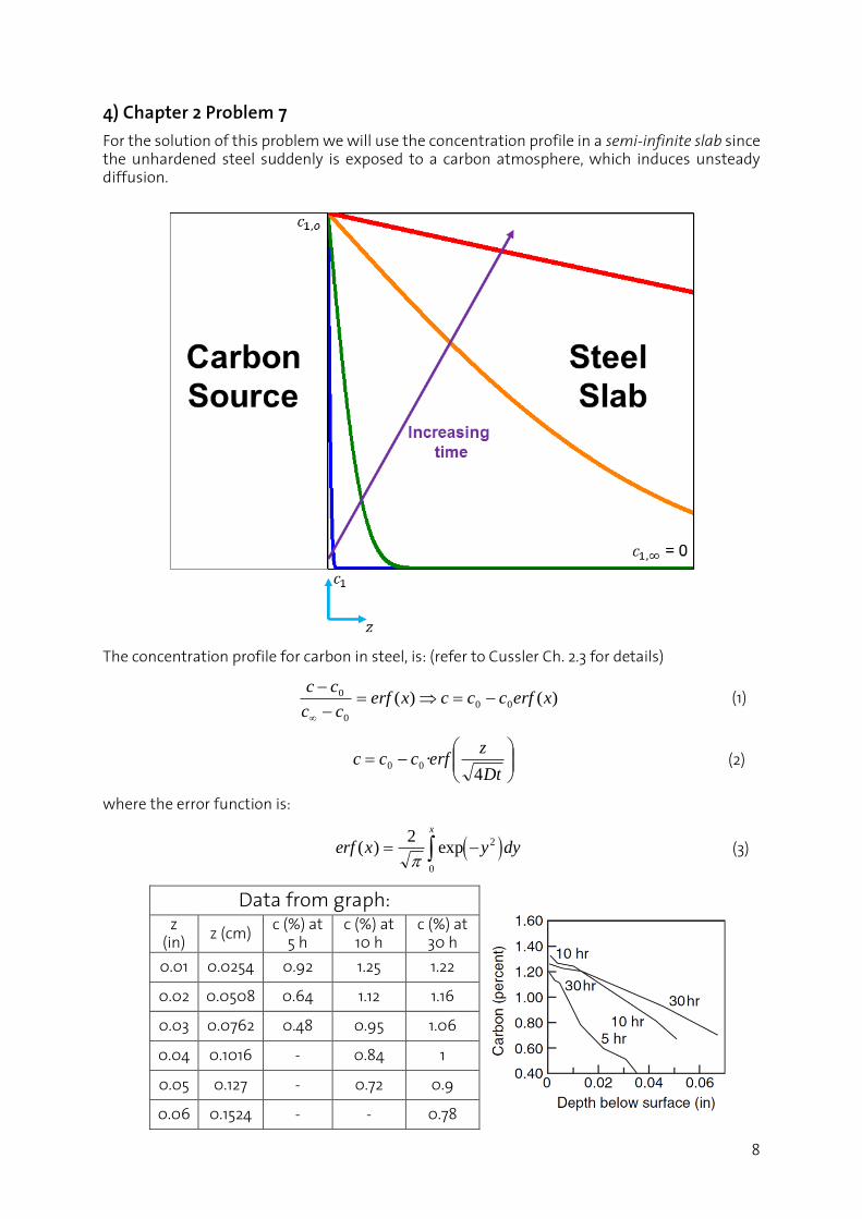
4) Chapter 2 Problem 7

For the solution of this problem we will use the concentration profile in a semi-infinite slab since the unhardened steel suddenly is exposed to a carbon atmosphere, which induces unsteady diffusion.

The concentration profile for carbon in steel, is: (refer to Cussler Ch. 2.3 for details)

)()( 00

0

0 xerfcccxerfcc

cc

(1)

Dt

zerfccc

4·00 (2)

where the error function is:

erf x y dy

x

( ) exp 2

0

2

(3)

Data from graph:

z (in)

z (cm) c (%) at

5 h c (%) at

10 h c (%) at

30 h

0.01 0.0254 0.92 1.25 1.22

0.02 0.0508 0.64 1.12 1.16

0.03 0.0762 0.48 0.95 1.06

0.04 0.1016 - 0.84 1

0.05 0.127 - 0.72 0.9

0.06 0.1524 - - 0.78

9

Observing the error function, we see that for very small x:

2·( )

xerf x

, since for y → 0, exp(-y2) = 1. (4)

Do not forget, that y is just a “dummy” variable for the integration. Therefore, replacing with:

4

zx

Dt (5)

we now get from (1):

tD

zcc

tD

zerfccc

·

4· 0000

(6)

We will use the linear approximation (6) to determine the diffusion coefficient from the graphs.

In other words, x approaches zero, either when z is small (we are close to the exposed face of the

steel slab), or when t is very long. Under such conditions, the concentration profile of carbon in

steel can be linear with respect to z (for a given, long, t) or with respect to t-1/2 (for a given, short,

z). In the above table we show values of carbon concentration at various locations (from the

exposed face) and times. If the given times are long enough, then the concentration profile

should be rather linear with z.

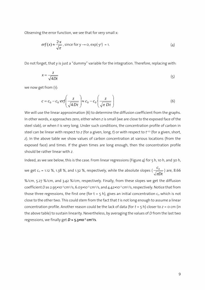
Indeed, as we see below, this is the case. From linear regressions (Figure 4) for 5 h, 10 h, and 30 h,

we get c0 = 1.12 %, 1.38 %, and 1.32 %, respectively, while the absolute slopes (Dt

c

0 ) are, 8.66

%/cm, 5.27 %/cm, and 3.42 %/cm, respectively. Finally, from these slopes we get the diffusion

coefficient D as 2.95×10-7 cm2/s, 6.03×10-7 cm2/s, and 4.42×10-7 cm2/s, respectively. Notice that from

those three regressions, the first one (for t = 5 h), gives an initial concentration c0 which is not

close to the other two. This could stem from the fact that t is not long enough to assume a linear

concentration profile. Another reason could be the lack of data (for t = 5 h) closer to z = 0 cm (in

the above table) to sustain linearity. Nevertheless, by averaging the values of D from the last two

regressions, we finally get D ≈ 5.3×10-7 cm2/s.

10

Linear regressions for t = 5 h (spheres), 10 h (squares), and 30 h (triangles).

11

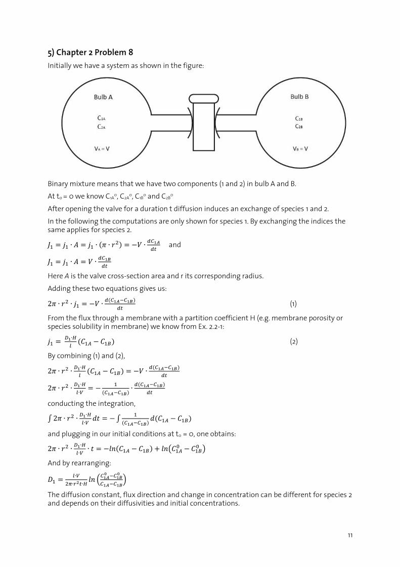
5) Chapter 2 Problem 8

Initially we have a system as shown in the figure:

Binary mixture means that we have two components (1 and 2) in bulb A and B.

At t0 = 0 we know C1A0, C2A

0, C1B0 and C2B

0

After opening the valve for a duration t diffusion induces an exchange of species 1 and 2.

In the following the computations are only shown for species 1. By exchanging the indices the same applies for species 2.

𝐽1 = 𝑗1 ∙ 𝐴 = 𝑗1 ∙ (𝜋 ∙ 𝑟2) = −𝑉 ∙𝑑𝐶1𝐴

𝑑𝑡 and

𝐽1 = 𝑗1 ∙ 𝐴 = 𝑉 ∙𝑑𝐶1𝐵

𝑑𝑡

Here A is the valve cross-section area and r its corresponding radius.

Adding these two equations gives us:

2𝜋 ∙ 𝑟2 ∙ 𝑗1 = −𝑉 ∙𝑑(𝐶1𝐴−𝐶1𝐵)

𝑑𝑡 (1)

From the flux through a membrane with a partition coefficient H (e.g. membrane porosity or species solubility in membrane) we know from Ex. 2.2-1:

𝑗1 = 𝐷1∙𝐻

𝑙(𝐶1𝐴 − 𝐶1𝐵) (2)

By combining (1) and (2),

2𝜋 ∙ 𝑟2 ∙𝐷1∙𝐻

𝑙(𝐶1𝐴 − 𝐶1𝐵) = −𝑉 ∙

𝑑(𝐶1𝐴−𝐶1𝐵)

𝑑𝑡

2𝜋 ∙ 𝑟2 ∙𝐷1∙𝐻

𝑙∙𝑉= −

1

(𝐶1𝐴−𝐶1𝐵)∙

𝑑(𝐶1𝐴−𝐶1𝐵)

𝑑𝑡

conducting the integration,

∫ 2𝜋 ∙ 𝑟2 ∙𝐷1∙𝐻

𝑙∙𝑉𝑑𝑡 = − ∫

1

(𝐶1𝐴−𝐶1𝐵)𝑑(𝐶1𝐴 − 𝐶1𝐵)

and plugging in our initial conditions at t0 = 0, one obtains:

2𝜋 ∙ 𝑟2 ∙𝐷1∙𝐻

𝑙∙𝑉∙ 𝑡 = −𝑙𝑛(𝐶1𝐴 − 𝐶1𝐵) + 𝑙𝑛(𝐶1𝐴

0 − 𝐶1𝐵0 )

And by rearranging:

𝐷1 =𝑙∙𝑉

2𝜋∙𝑟2𝑡∙𝐻𝑙𝑛 (

𝐶1𝐴0 −𝐶1𝐵

0

𝐶1𝐴−𝐶1𝐵)

The diffusion constant, flux direction and change in concentration can be different for species 2 and depends on their diffusivities and initial concentrations.