15. Lecture WS 2008/09Bioinformatics III1 V15 Stochastic simulations of cellular signalling Introduction into stochastic processes, see e.g. Nico van Kampen‘s

15. Lecture WS 2008/09

Bioinformatics III 1

V15 Stochastic simulations of cellular signalling

Introduction into stochastic processes,

see e.g. Nico van Kampen‘s book

A random number or stochastic variable is an

object X defined by

(a) a set of possible values (called „range“, „set of states“,

„sample space“, or „phase space“) and

(b) a probability distribution over this set.

Ad (a) The set may be discrete, e.g. head or tails, or the number of molecules of a

certain component in a reacting mixture.

Or the set may be continuous in a given interval as the velocity of a Brownian

particle. Or it may be partly discrete, partly continuous.

The set of states may also be multidimensional. Then, X stands for a vector X.



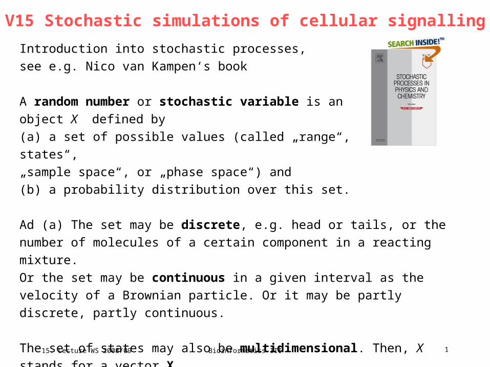
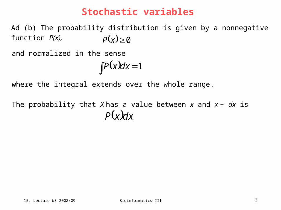
Stochastic variables

Ad (b) The probability distribution is given by a nonnegative function P(x),

0xPand normalized in the sense

1dxxP

where the integral extends over the whole range.

The probability that X has a value between x and x + dx is

dxxP



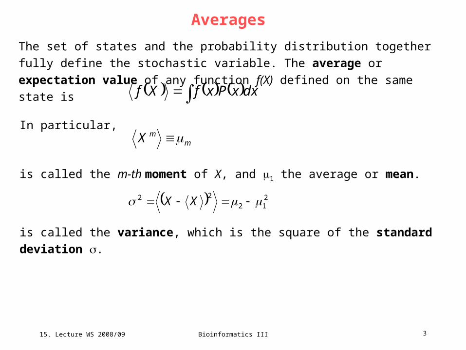
Averages

The set of states and the probability distribution together fully define the stochastic

variable. The average or expectation value of any function f(X) defined on the

same state is dxxPxfXf

In particular,

mmX

is called the m-th moment of X, and 1 the average or mean.

212

22 XX

is called the variance, which is the square of the standard deviation .



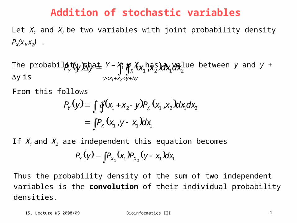
Addition of stochastic variables

Let X1 and X2 be two variables with joint probability density PX(x1,x2) .

The probability that Y = X1 + X2 has a value between y and y + y is

yyxxy

XY dxdxxxPyyP21

2121 ,

From this follows

111

212121

,

,

dxxyxP

dxdxxxPyxxyP

X

XY

If X1 and X2 are independent this equation becomes

111 21dxxyPxPyP XXY

Thus the probability density of the sum of two independent variables is the

convolution of their individual probability densities.



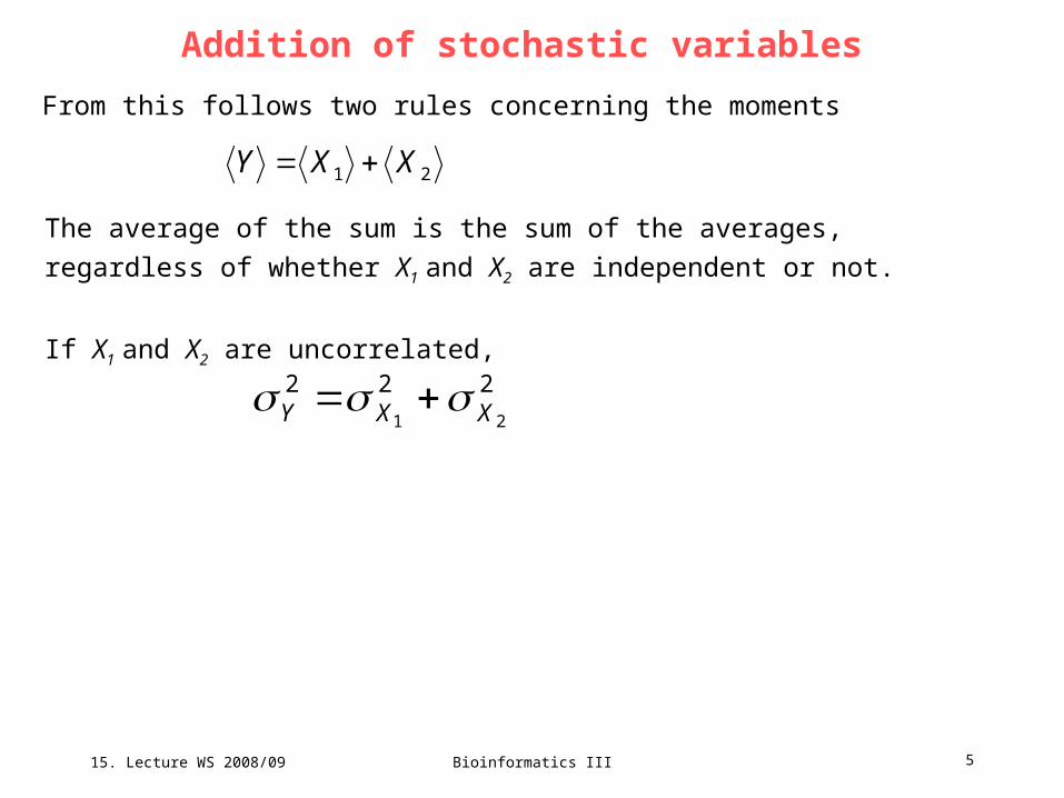
Addition of stochastic variables

From this follows two rules concerning the moments

21 XXY

The average of the sum is the sum of the averages,

regardless of whether X1 and X2 are independent or not.

If X1 and X2 are uncorrelated,222

21 XXY



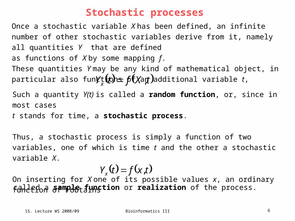
Stochastic processes Once a stochastic variable X has been defined, an infinite number of other

stochastic variables derive from it, namely all quantities Y that are defined

as functions of X by some mapping f.

These quantities Y may be any kind of mathematical object, in particular also

functions of an additional variable t,

Such a quantity Y(t) is called a random function, or, since in most cases

t stands for time, a stochastic process.

Thus, a stochastic process is simply a function of two variables, one of which is

time t and the other a stochastic variable X.

On inserting for X one of its possible values x, an ordinary function of t obtains

called a sample function or realization of the process.

tXftYx ,

txftYx ,



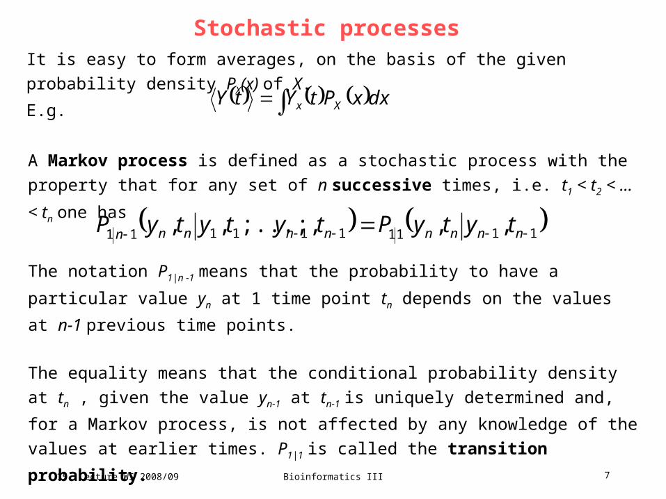
Stochastic processes It is easy to form averages, on the basis of the given probability density PX(x) of X.

E.g. dxxPtYtY Xx

A Markov process is defined as a stochastic process with the property that for any

set of n successive times, i.e. t1 < t2 < ... < tn one has

1111111111 ,,,;...;,, nnnnnnnnn tytyPtytytyP

The notation P1|n -1 means that the probability to have a particular value yn at 1 time

point tn depends on the values at n-1 previous time points.

The equality means that the conditional probability density at tn , given the value yn-1

at tn-1 is uniquely determined and, for a Markov process, is not affected by any

knowledge of the values at earlier times. P1|1 is called the transition probability.



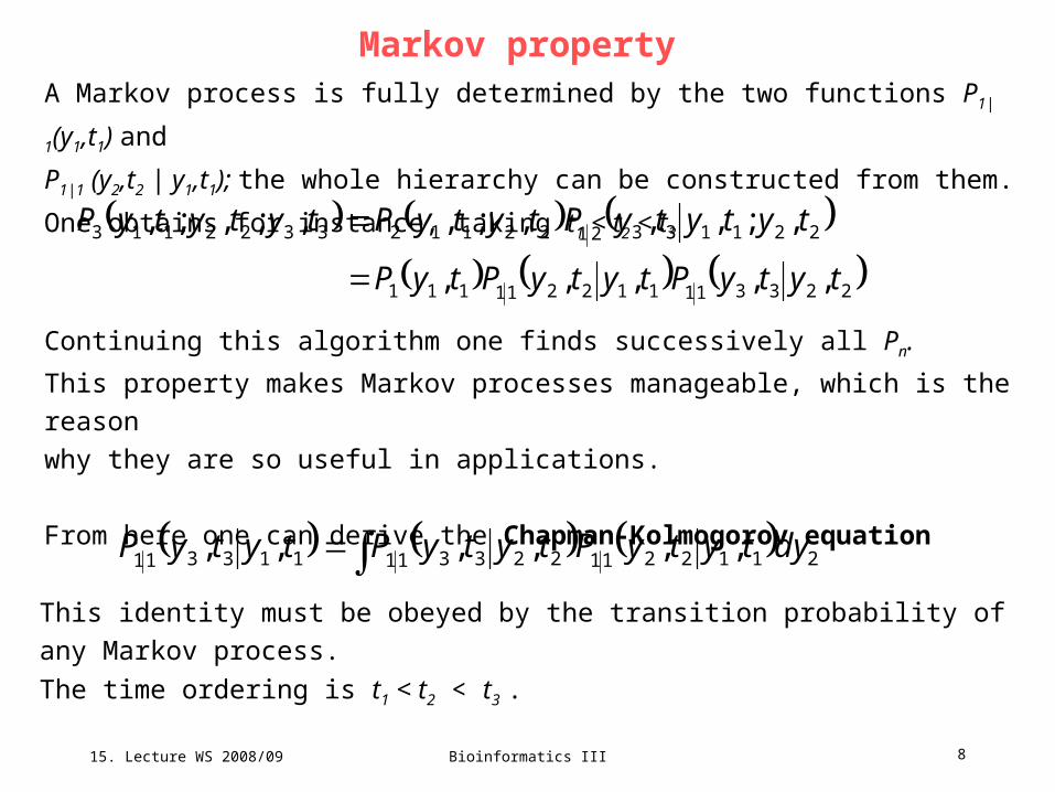
Markov property A Markov process is fully determined by the two functions P1|1(y1,t1) and

P1|1 (y2,t2 | y1,t1); the whole hierarchy can be constructed from them.

One obtains for instance, taking t1 < t2 < t3

Continuing this algorithm one finds successively all Pn.

This property makes Markov processes manageable, which is the reason

why they are so useful in applications.

From here one can derive the Chapman-Kolmogorov equation

223311112211111

22113321221123322113

,,,,,

,;,,,;,,;,;,

tytyPtytyPtyP

tytytyPtytyPtytytyP

2112211223311113311 ,,,,,, dytytyPtytyPtytyP

This identity must be obeyed by the transition probability of any Markov process.

The time ordering is t1 < t2 < t3 .



Master equation

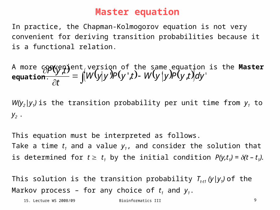
In practice, the Chapman-Kolmogorov equation is not very convenient for deriving

transition probabilities because it is a functional relation.

A more convenient version of the same equation is the Master equation.

W(y2|y1) is the transition probability per unit time from y1 to y2 .

This equation must be interpreted as follows.

Take a time t1 and a value y1, and consider the solution that is determined for t t1

by the initial condition P(y,t1) = (t – t1).

This solution is the transition probability Tt-t1 (y|y1) of the Markov process – for any

choice of t1 and y1.

',','',

dytyPyyWtyPyyWt

tyP



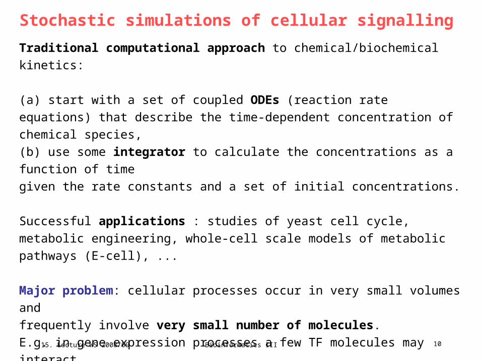
Stochastic simulations of cellular signalling

Traditional computational approach to chemical/biochemical kinetics:

(a) start with a set of coupled ODEs (reaction rate equations) that describe the

time-dependent concentration of chemical species,

(b) use some integrator to calculate the concentrations as a function of time

given the rate constants and a set of initial concentrations.

Successful applications : studies of yeast cell cycle, metabolic engineering,

whole-cell scale models of metabolic pathways (E-cell), ...

Major problem: cellular processes occur in very small volumes and

frequently involve very small number of molecules.

E.g. in gene expression processes a few TF molecules may interact

with a single gene regulatory region.

E.coli cells contain on average only 10 molecules of Lac repressor.



Include stochastic effects

(Consequence1) modeling of reactions as continuous fluxes of matter

is no longer correct.

(Consequence2) Significant stochastic fluctuations occur.

To study the stochastic effects in biochemical reactions stochastic formulations

of chemical kinetics and Monte Carlo computer simulations have been used.

Daniel Gillespie (J Comput Phys 22, 403 (1976); J Chem Phys 81, 2340 (1977))

introduced the exact Dynamic Monte Carlo (DMC) method that connects the

traditional chemical kinetics and stochastic approaches.

Assuming that the system is well mixed, the rate constants appearing in these two

methods are related.



Dynamic Monte Carlo

In the usual implementation of DMC for kinetic simulations, each reaction is

considered as an event and each event has an associated probability of occurring.

The probability P(Ei) that a certain chemical reaction Ei takes place in a given time

interval t is proportional to an effective rate constant k and to the number of

chemical species that can take part in that event.

E.g. the probability of the first-order reaction

X Y + Z

would be k1Nx with Nx :number of species X, and

k1 : rate constant of the reaction

Similarly, the probability of the reverse second-order reaction

Y + Z X

would be k2NYNZ.

Resat et al., J.Phys.Chem. B 105, 11026 (2001)



Dynamic Monte Carlo

As the method is a probabilistic approach based on „events“, „reactions“ included in

the DMC simulations do not have to be solely chemical reactions.

Any process that can be associated with a probability

can be included as an event in the DMC simulations.

E.g. a substrate attaching to a solid surface can initiate

a series of chemical reactions.

One can split the modelling into

- the physical events of substrate arrival,

- attaching the substrate,

- followed by the chemical reaction steps.




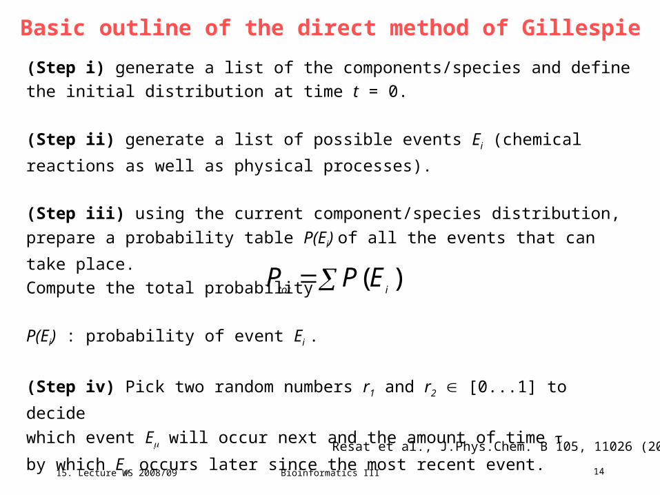
Basic outline of the direct method of Gillespie

(Step i) generate a list of the components/species and define the initial distribution

at time t = 0.

(Step ii) generate a list of possible events Ei (chemical reactions as well as

physical processes).

(Step iii) using the current component/species distribution, prepare a probability

table P(Ei) of all the events that can take place.

Compute the total probability

P(Ei) : probability of event Ei .

(Step iv) Pick two random numbers r1 and r2 [0...1] to decide

which event E will occur next and the amount of time

by which E occurs later since the most recent event.


)(itotEPP



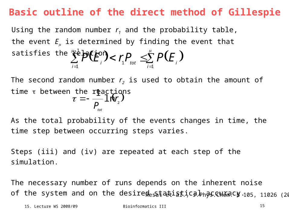
Basic outline of the direct method of Gillespie

Using the random number r1 and the probability table,

the event E is determined by finding the event that satisfies the relation


1

1

11

ii

itoti

EPPrEP

The second random number r2 is used to obtain the amount of time between the

reactions

2ln

1r

Ptot

As the total probability of the events changes in time, the time step between

occurring steps varies.

Steps (iii) and (iv) are repeated at each step of the simulation.

The necessary number of runs depends on the inherent noise

of the system and on the desired statistical accuracy.



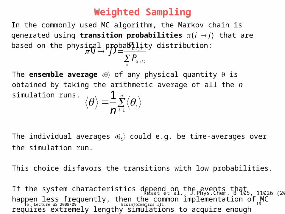
Weighted SamplingIn the commonly used MC algorithm, the Markov chain is generated using

transition probabilities (i j) that are based on the physical probability

distribution:


kki

ji

P

Pji

The ensemble average of any physical quantity is obtained by taking the

arithmetic average of all the n simulation runs.

The individual averages i could e.g. be time-averages over the simulation run.

This choice disfavors the transitions with low probabilities.

If the system characteristics depend on the events that happen less frequently,

then the common implementation of MC requires extremely lengthy simulations to

acquire enough statistical sampling.

n

iin 1

1



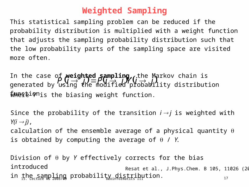
Weighted SamplingThis statistical sampling problem can be reduced if the probability distribution is

multiplied with a weight function that adjusts the sampling probability distribution

such that the low probability parts of the sampling space are visited more often.

In the case of weighted sampling, the Markov chain is generated by using the

modified probability distribution function


jiYjiPjiPw

where Y is the biasing weight function.

Since the probability of the transition i j is weighted with Y(i j),

calculation of the ensemble average of a physical quantity

is obtained by computing the average of / Y.

Division of by Y effectively corrects for the bias introduced

in the sampling probability distribution.



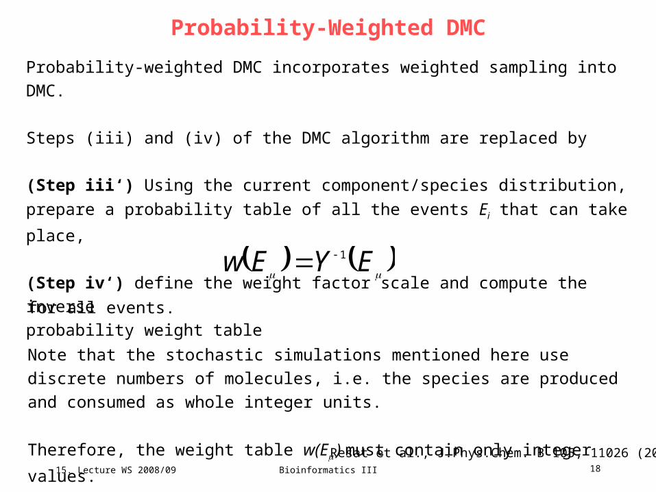
Probability-Weighted DMC

Probability-weighted DMC incorporates weighted sampling into DMC.

Steps (iii) and (iv) of the DMC algorithm are replaced by

(Step iii‘) Using the current component/species distribution,

prepare a probability table of all the events Ei that can take place,

(Step iv‘) define the weight factor scale and compute the inverse

probability weight table


EYEw 1

for all events.

Note that the stochastic simulations mentioned here use discrete numbers of

molecules, i.e. the species are produced and consumed as whole integer units.

Therefore, the weight table w(E ) must contain only integer values.



Probability-Weighted DMC

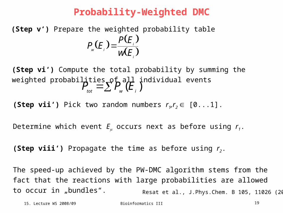
(Step v‘) Prepare the weighted probability table


i

i

iw Ew

EPEP

(Step vi‘) Compute the total probability by summing the weighted probabilities of all

individual events )(

iwtotEPP

(Step vii‘) Pick two random numbers r1,r2 [0...1].

Determine which event E occurs next as before using r1.

(Step viii‘) Propagate the time as before using r2.

The speed-up achieved by the PW-DMC algorithm stems from the fact that the

reactions with large probabilities are allowed to occur in „bundles“.



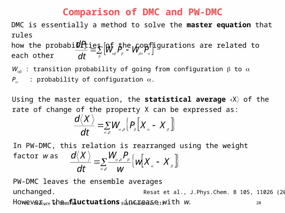
Comparison of DMC and PW-DMCDMC is essentially a method to solve the master equation that rules

how the probabilities of the configurations are related to each other


PWPWdt

dP

W : transition probability of going from configuration to

P : probability of configuration .

Using the master equation, the statistical average X of the rate of change of the

property X can be expressed as:

,

,XXPW

dt

Xd

In PW-DMC, this relation is rearranged using the weight factor w as

,

, XXww

PW

dt

Xd

PW-DMC leaves the ensemble averages unchanged.

However, the fluctuations increase with w.



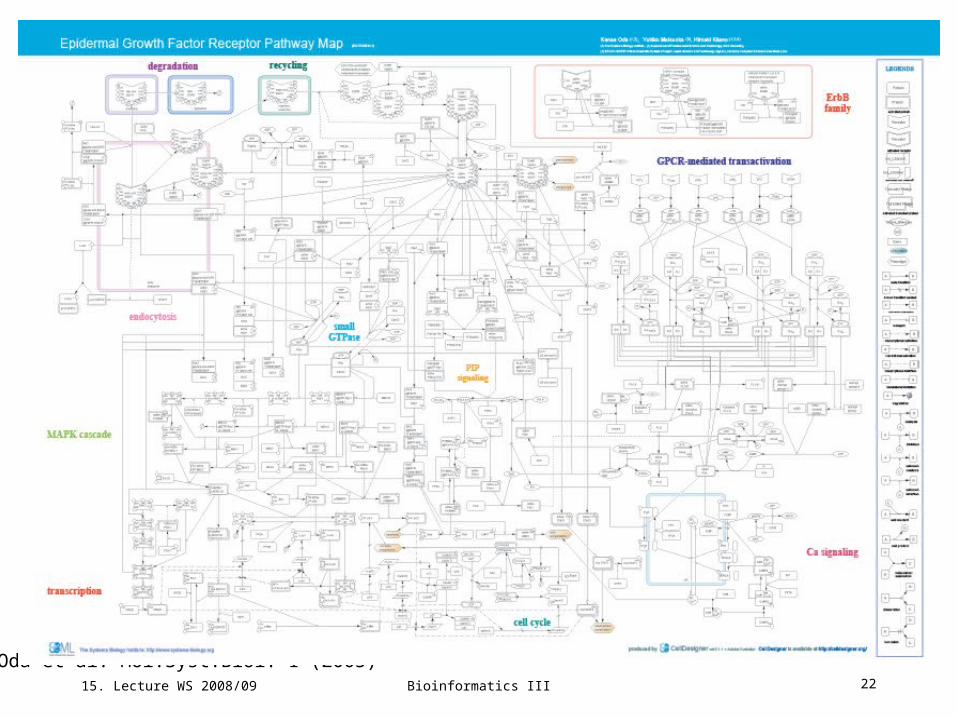
Epidermal growth factor receptor signaling pathway

The EGFR signaling pathway is one of the most important pathways that regulate

growth, survival, proliferation, and differentiation in mammalian cells.

International consortium has assembled a comprehensive pathway map including

- EGFR endocytosis followed by its degradation or recycling,

- small GTPase-mediated signal transduction such as MAPK cascade, PIP

signaling, cell cycle, and GPCR-mediated EGFR transactivation via intracellular

Ca2+ signalling.

Map includes 211 reactions and 322 species taking part in reactions.

Species: 202 proteins, 3 ions, 21 simple molecules, 73 oligomers, 7 genes, 7 RNAs.

Proteins: 122 molecules including 10 ligands, 10 receptors, 61 enzymes (including 32 kinases), 3 ion

channels, 10 transcription factors, 6 G protein subunits, 22 adaptor proteins.

Reactions: 131 state transitions, 34 transportations, 32 associations, 11 dissociations, 2 truncations.

Oda et al. Mol.Syst.Biol. 1 (2005)






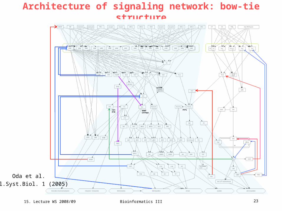
Architecture of signaling network: bow-tie structure

Oda et al.

Mol.Syst.Biol. 1 (2005)



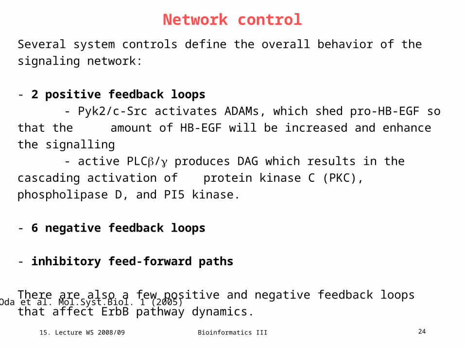
Network control

Several system controls define the overall behavior of the signaling network:

- 2 positive feedback loops

- Pyk2/c-Src activates ADAMs, which shed pro-HB-EGF so that the

amount of HB-EGF will be increased and enhance the signalling

- active PLC/ produces DAG which results in the cascading activation

of protein kinase C (PKC), phospholipase D, and PI5 kinase.

- 6 negative feedback loops

- inhibitory feed-forward paths

There are also a few positive and negative feedback loops that affect ErbB

pathway dynamics.




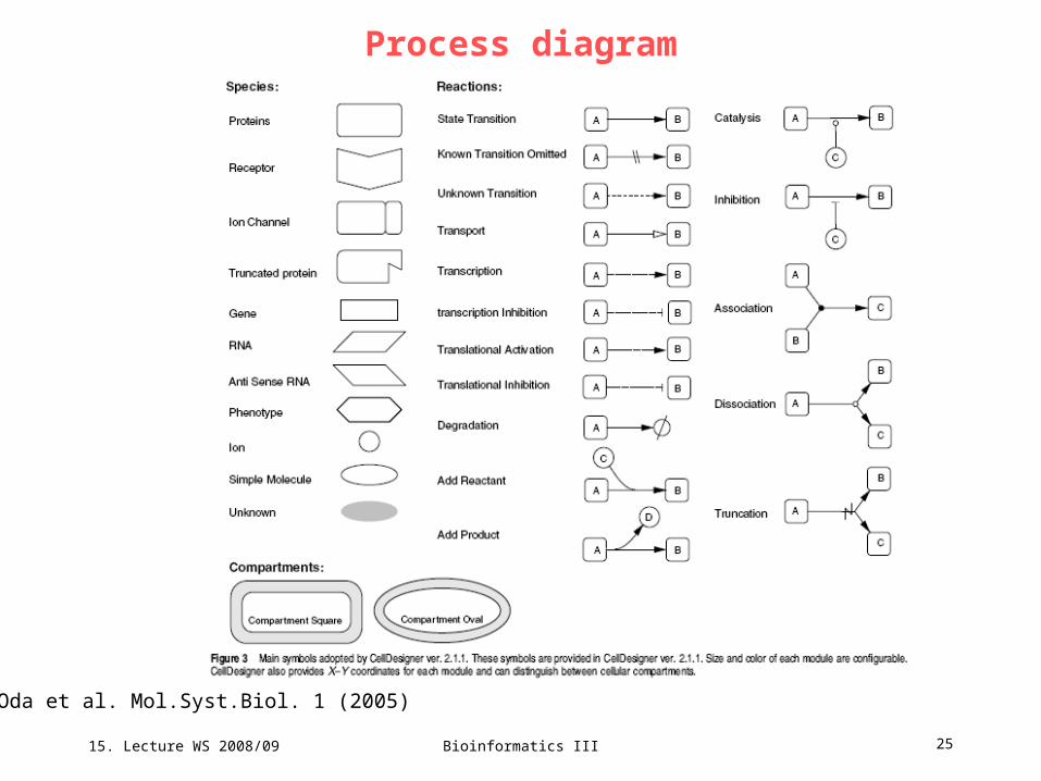
Process diagram




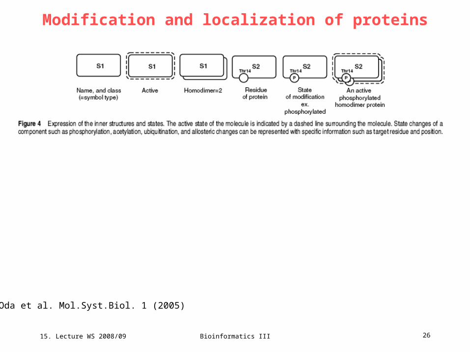
Modification and localization of proteins




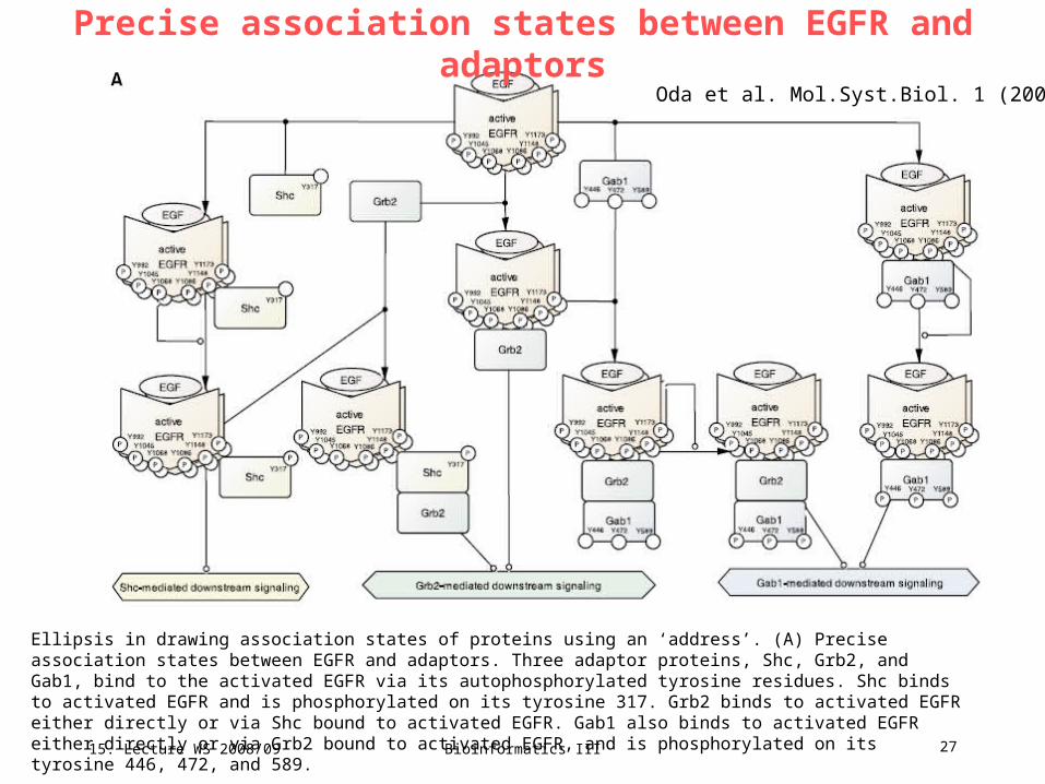
Precise association states between EGFR and adaptorsOda et al. Mol.Syst.Biol. 1 (2005)

Ellipsis in drawing association states of proteins using an ‘address’. (A) Precise association states between EGFR and adaptors. Three adaptor proteins, Shc, Grb2, and Gab1, bind to the activated EGFR via its autophosphorylated tyrosine residues. Shc binds to activated EGFR and is phosphorylated on its tyrosine 317. Grb2 binds to activated EGFR either directly or via Shc bound to activated EGFR. Gab1 also binds to activated EGFR either directly or via Grb2 bound to activated EGFR, and is phosphorylated on its tyrosine 446, 472, and 589.



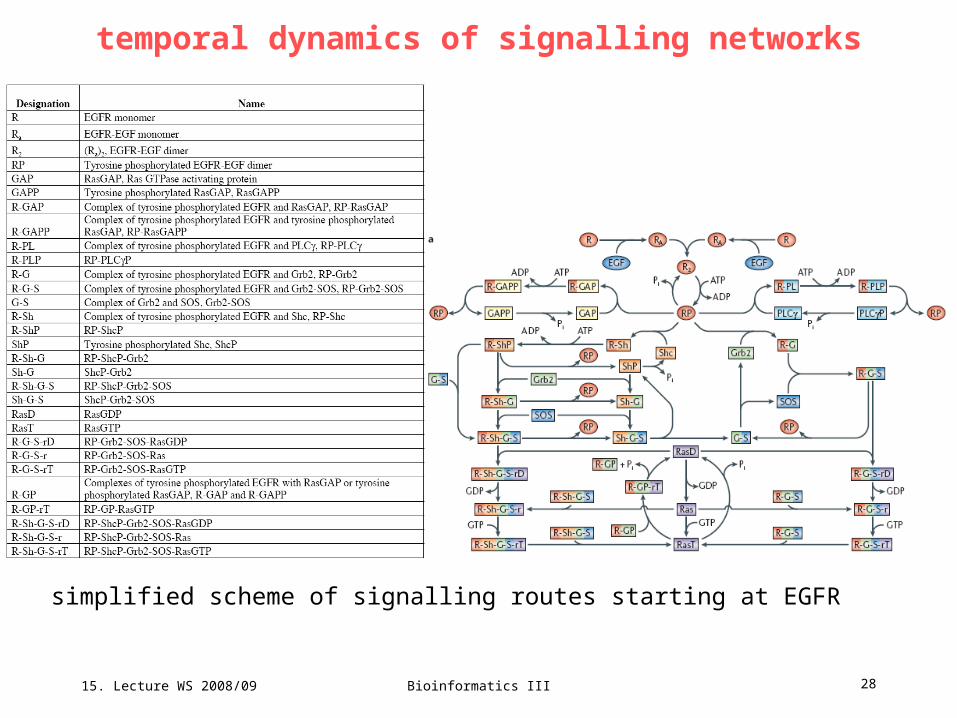
temporal dynamics of signalling networks

simplified scheme of signalling routes starting at EGFR



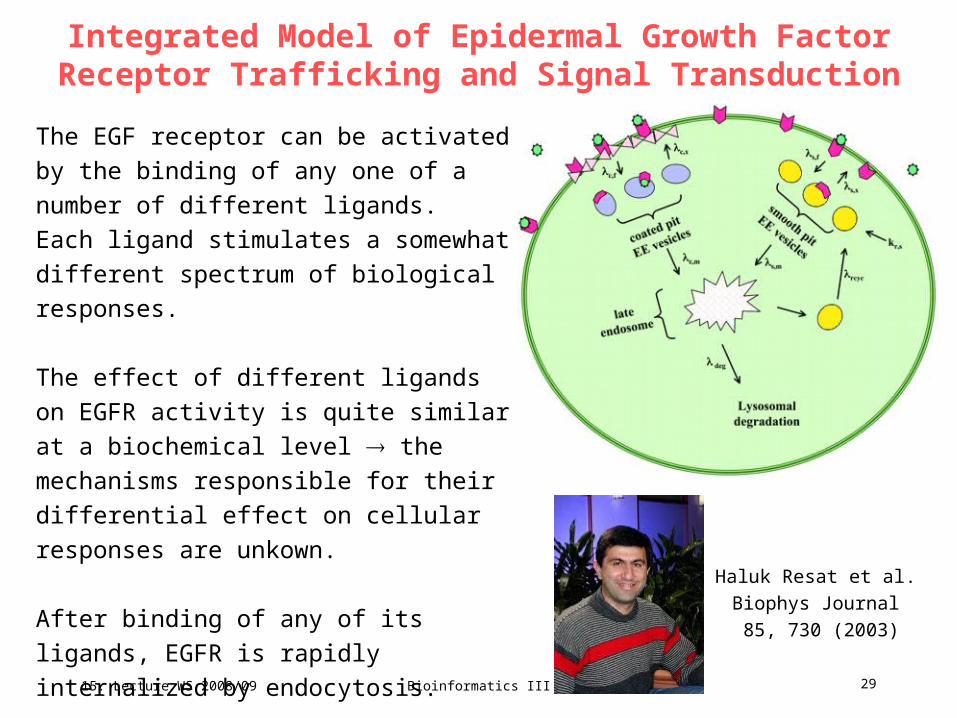
Integrated Model of Epidermal Growth Factor Receptor Trafficking and Signal Transduction

The EGF receptor can be activated by the

binding of any one of a number of different

ligands.

Each ligand stimulates a somewhat different

spectrum of biological responses.

The effect of different ligands on EGFR

activity is quite similar at a biochemical level

the mechanisms responsible for their

differential effect on cellular responses are

unkown.

After binding of any of its ligands, EGFR is

rapidly internalized by endocytosis. Haluk Resat et al.

Biophys Journal

85, 730 (2003)



Computational modelling of EGF receptor system

(1) trafficking and ligand-induced endocytosis

(2) signaling through Ras or MAP kinases

This work combines both aspects into a single model.

Most approaches to building computational kinetic models have severe

drawbacks when representing spatially heterogenous processes on a cellular

scale.

Review: In the traditional approach, we

- formulate set of coupled ODEs (reaction rate equations) for the time-dependent

concentration of chemical species

- use integrator to propagate the concentrations as a function of time given the

rate constants and a set of initial concentrations.

Resat et al. Biophys Journal 85, 730 (2003)



Multiple time scale problem

In Dynamic Monte Carlo, reactions are considered events that occur with certain

probabilities over set intervals of time.

The event probabilities depend on the rate constant of the reaction and on the

number of molecules participating in the reaction.

In many interesting natural problems, the time scales of the events are spread

over a large spectrum.

Therefore it is very inefficient to treat all processes at the time scale of the fastest

individual reaction.

In the EGFR signaling network,

- receptor phosphorylation after ligand binding occurs almost instantaneously

- vesicle formation or sorting to lysosomes requires many minutes.




Solution to multiple time scale problem

Computing millions and billions non-correlated random numbers

can become a time-consuming process.

Resat et al. (2001) introduced Probability-Weighted DMC to speed-up the

simulation by factor 20 – 100.

Different processes are only tested at variant times depending on their

probabilities

very unlikely processes compute MC decision very infrequently.




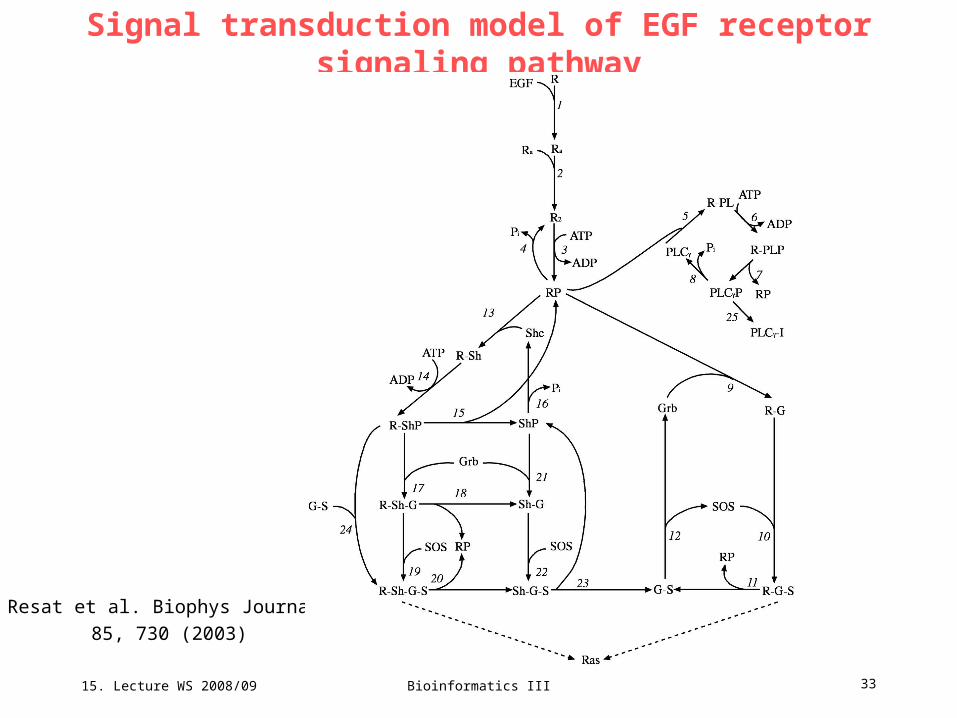
Signal transduction model of EGF receptor signaling pathway

Resat et al. Biophys Journal

85, 730 (2003)



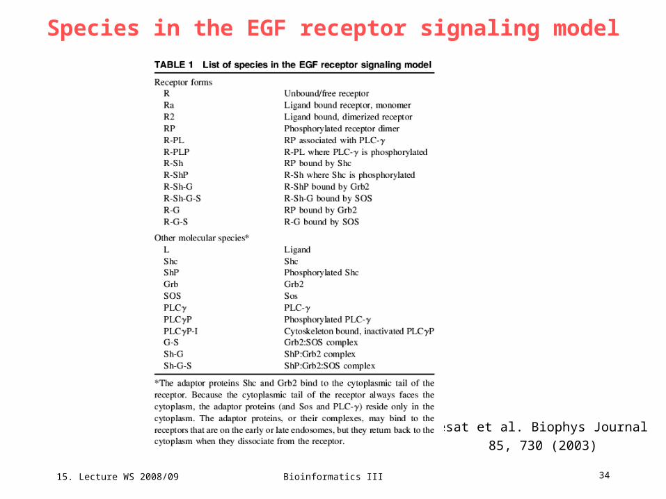
Species in the EGF receptor signaling model

Resat et al. Biophys Journal

85, 730 (2003)



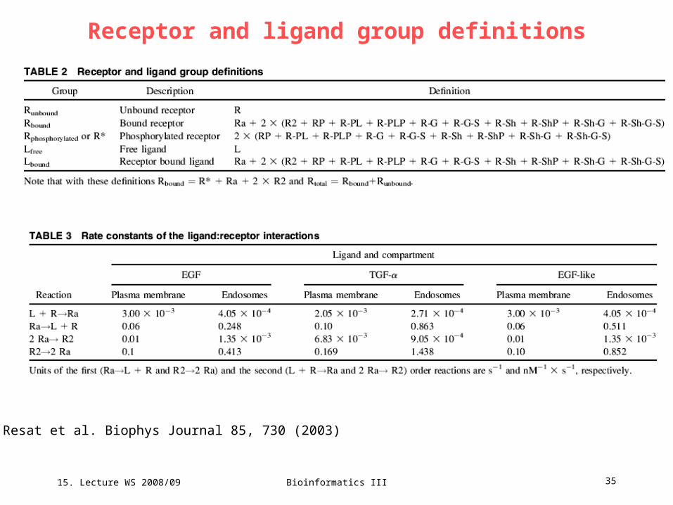
Receptor and ligand group definitions




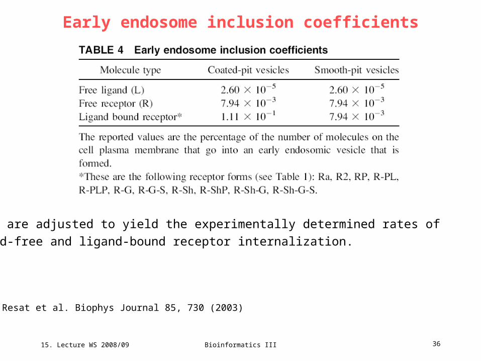
Early endosome inclusion coefficients


These are adjusted to yield the experimentally determined rates of

ligand-free and ligand-bound receptor internalization.



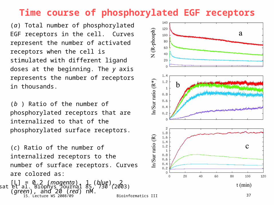
Time course of phosphorylated EGF receptors(a) Total number of phosphorylated EGF

receptors in the cell. Curves represent the

number of activated receptors when the cell is

stimulated with different ligand doses at the

beginning. The y axis represents the number of

receptors in thousands.

(b ) Ratio of the number of phosphorylated

receptors that are internalized to that of the

phosphorylated surface receptors.

(c) Ratio of the number of internalized

receptors to the number of surface receptors.

Curves are colored as:

[L] = 0.2 (magenta), 1 (blue), 2 (green), and 20

(red) nM.




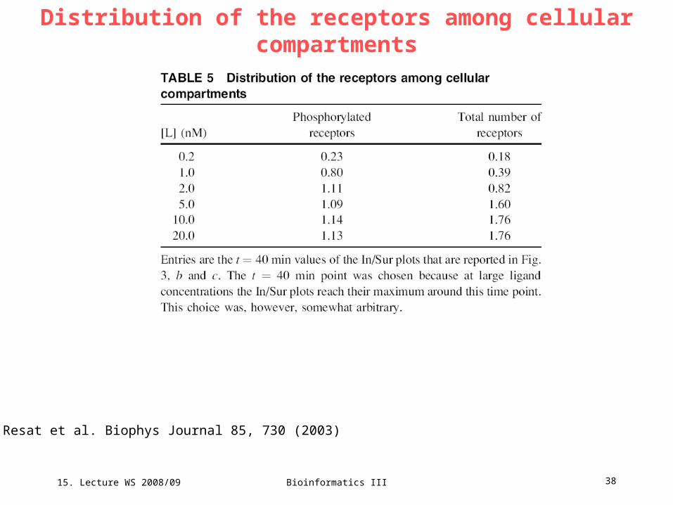
Distribution of the receptors among cellular compartments




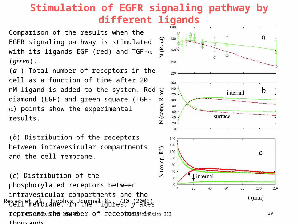
Stimulation of EGFR signaling pathway by different ligands

Comparison of the results when the EGFR

signaling pathway is stimulated with its ligands

EGF (red) and TGF- (green).

(a ) Total number of receptors in the cell as a

function of time after 20 nM ligand is added to the

system. Red diamond (EGF) and green square

(TGF-) points show the experimental results.

(b) Distribution of the receptors between

intravesicular compartments and the cell

membrane.

(c) Distribution of the phosphorylated receptors

between intravesicular compartments and the cell

membrane. In the figures, y axes represent the

number of receptors in thousands.




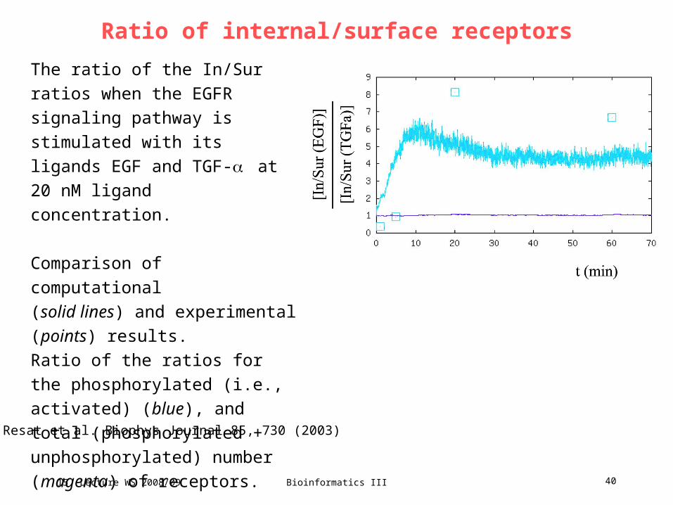
Ratio of internal/surface receptors

The ratio of the In/Sur ratios when

the EGFR signaling pathway is

stimulated with its ligands EGF and

TGF- at 20 nM ligand

concentration.

Comparison of computational

(solid lines) and experimental

(points) results.

Ratio of the ratios for the

phosphorylated (i.e., activated)

(blue), and total (phosphorylated +

unphosphorylated) number

(magenta) of receptors.




SummaryLarge-scale simulations of the kinetics of biological signaling networks are

becoming feasible.

Here, the model of the EGFR trafficking consisted of hundreds of distinct

compartments and ca. 13.000 reactions/events that occur on a wide spatial-

temporal range.

The exact Dynamic Monte Carlo algorithm of Gillespie (1976/1977) was a

breakthrough for simulations of stochastic systems.

Problem: simulations can become very time-consuming. In particular if the

processes occur on different time scales.

Methods like the probability-weighted DMC are promising tools for studying

complex cellular systems using molecular quanta.

V16: more on stochastic dynamics simulations.

Documents

15. Lecture WS 2008/09Bioinformatics III1 V15 Stochastic simulations of cellular signalling Introduction into stochastic processes, see e.g. Nico van Kampen‘s