Embed Size (px)
DESCRIPTION
15-826: Multimedia Databases and Data Mining. Lecture #25: Time series mining and forecasting Christos Faloutsos. Must-Read Material. - PowerPoint PPT Presentation
Citation preview
CMU SCS
15-826: Multimedia Databasesand Data Mining
Lecture #25: Time series mining and forecasting
Christos Faloutsos
CMU SCS
15-826 (c) C. Faloutsos, 2012 2
Must-Read Material• Byong-Kee Yi, Nikolaos D. Sidiropoulos,
Theodore Johnson, H.V. Jagadish, Christos Faloutsos and Alex Biliris, Online Data Mining for Co-Evolving Time Sequences, ICDE, Feb 2000.
• Chungmin Melvin Chen and Nick Roussopoulos, Adaptive Selectivity Estimation Using Query Feedbacks, SIGMOD 1994
CMU SCS
15-826 (c) C. Faloutsos, 2012 3
Thanks
Deepay Chakrabarti (CMU)
Spiros Papadimitriou (CMU)
Prof. Byoung-Kee Yi (Pohang U.)
Prof. Dimitris Gunopulos (UCR)
Mengzhi Wang (CMU)
CMU SCS
15-826 (c) C. Faloutsos, 2012 4
Outline
• Motivation
• Similarity search – distance functions
• Linear Forecasting
• Bursty traffic - fractals and multifractals
• Non-linear forecasting
• Conclusions
CMU SCS
15-826 (c) C. Faloutsos, 2012 5
Problem definition
• Given: one or more sequences x1 , x2 , … , xt , …
(y1, y2, … , yt, …
… )
• Find – similar sequences; forecasts– patterns; clusters; outliers
CMU SCS
15-826 (c) C. Faloutsos, 2012 6
Motivation - Applications• Financial, sales, economic series
• Medical
– ECGs +; blood pressure etc monitoring
– reactions to new drugs
– elderly care
CMU SCS
15-826 (c) C. Faloutsos, 2012 7
Motivation - Applications (cont’d)
• ‘Smart house’
– sensors monitor temperature, humidity, air quality
• video surveillance
CMU SCS
15-826 (c) C. Faloutsos, 2012 8
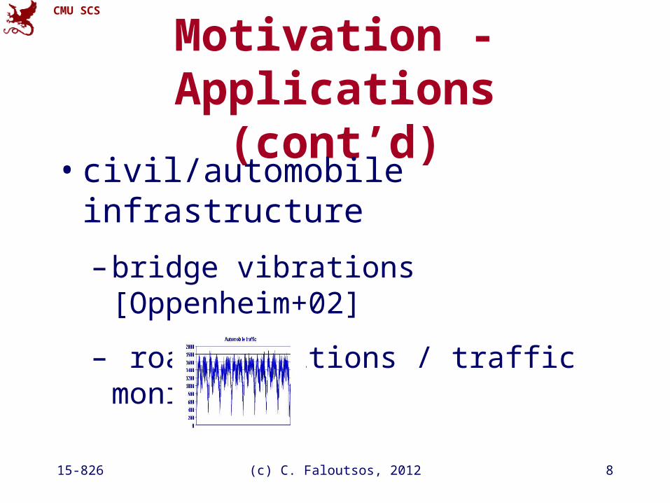
Motivation - Applications (cont’d)
• civil/automobile infrastructure
– bridge vibrations [Oppenheim+02]
– road conditions / traffic monitoring
CMU SCS
15-826 (c) C. Faloutsos, 2012 9
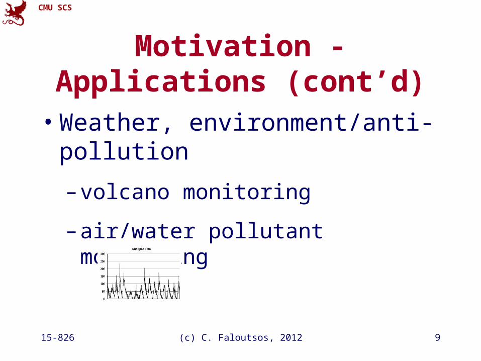
Motivation - Applications (cont’d)
• Weather, environment/anti-pollution
– volcano monitoring
– air/water pollutant monitoring
CMU SCS
15-826 (c) C. Faloutsos, 2012 10
Motivation - Applications (cont’d)
• Computer systems
– ‘Active Disks’ (buffering, prefetching)
– web servers (ditto)
– network traffic monitoring
– ...
CMU SCS
15-826 (c) C. Faloutsos, 2012 11
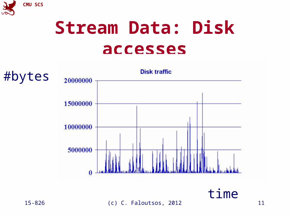
Stream Data: Disk accesses
time
#bytes
CMU SCS
15-826 (c) C. Faloutsos, 2012 12
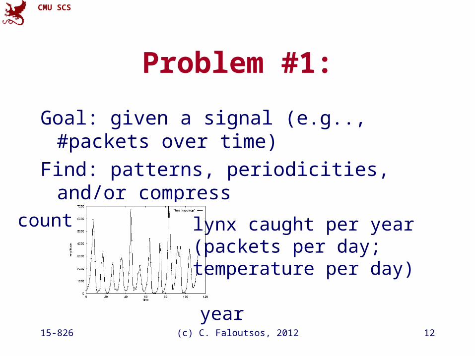
Problem #1:
Goal: given a signal (e.g.., #packets over time)
Find: patterns, periodicities, and/or compress
year
count lynx caught per year(packets per day;temperature per day)
CMU SCS
15-826 (c) C. Faloutsos, 2012 13
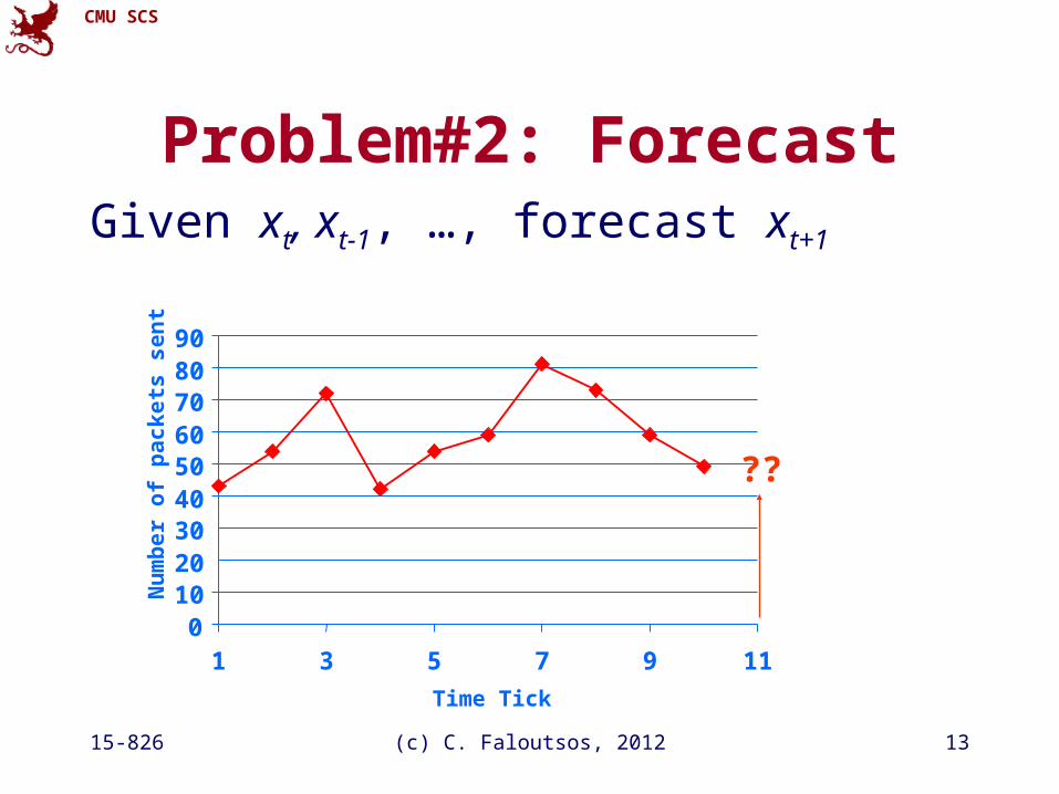
Problem#2: ForecastGiven xt, xt-1, …, forecast xt+1
0102030405060708090
1 3 5 7 9 11
Time Tick
Nu
mb
er o
f p
ack
ets
sen
t
??
CMU SCS
15-826 (c) C. Faloutsos, 2012 14
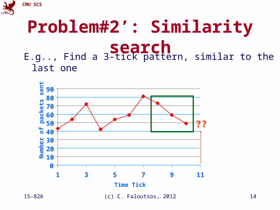
Problem#2’: Similarity searchE.g.., Find a 3-tick pattern, similar to the last one
0102030405060708090
1 3 5 7 9 11
Time Tick
Nu
mb
er o
f p
ack
ets
sen
t
??
CMU SCS
15-826 (c) C. Faloutsos, 2012 15
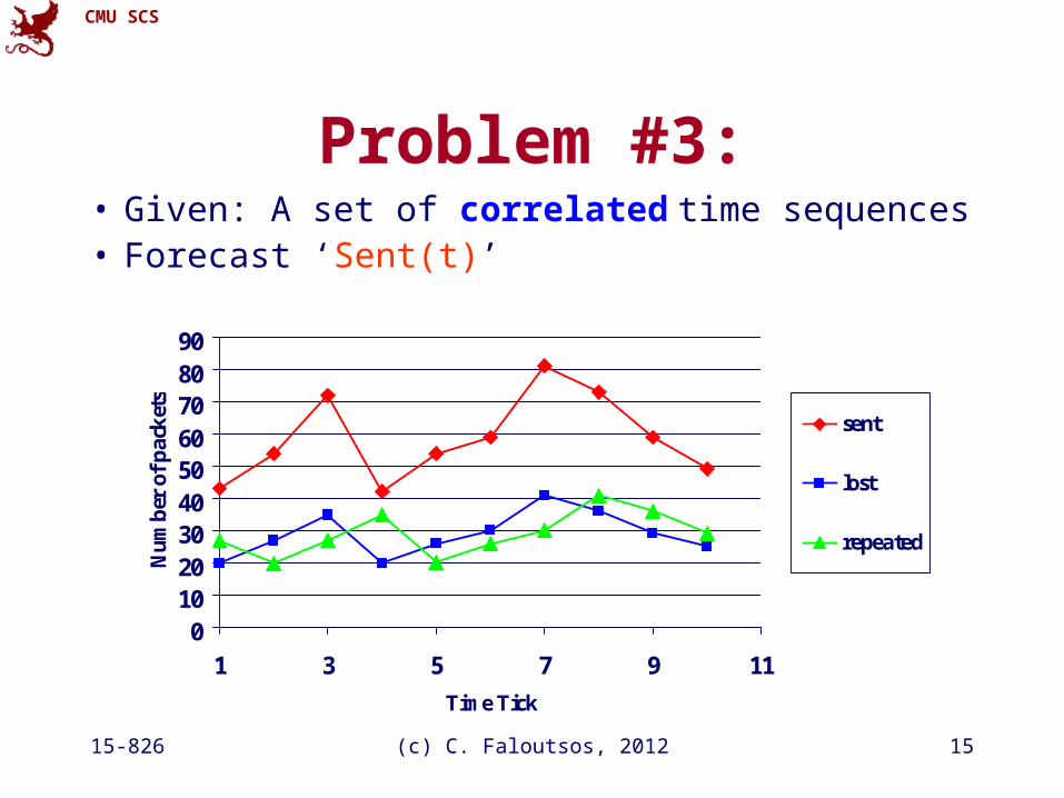
Problem #3:• Given: A set of correlated time sequences• Forecast ‘Sent(t)’
0102030405060708090
1 3 5 7 9 11
Time Tick
Nu
mb
er o
f p
ack
ets
sent
lost
repeated
CMU SCS
15-826 (c) C. Faloutsos, 2012 16
Important observations
Patterns, rules, forecasting and similarity indexing are closely related:
• To do forecasting, we need– to find patterns/rules– to find similar settings in the past
• to find outliers, we need to have forecasts– (outlier = too far away from our forecast)
CMU SCS
15-826 (c) C. Faloutsos, 2012 17
Outline
• Motivation
• Similarity Search and Indexing
• Linear Forecasting
• Bursty traffic - fractals and multifractals
• Non-linear forecasting
• Conclusions
CMU SCS
15-826 (c) C. Faloutsos, 2012 18
Outline
• Motivation
• Similarity search and distance functions– Euclidean– Time-warping
• ...
CMU SCS
15-826 (c) C. Faloutsos, 2012 19
Importance of distance functions
Subtle, but absolutely necessary:
• A ‘must’ for similarity indexing (-> forecasting)
• A ‘must’ for clustering
Two major families– Euclidean and Lp norms– Time warping and variations
CMU SCS
15-826 (c) C. Faloutsos, 2012 20
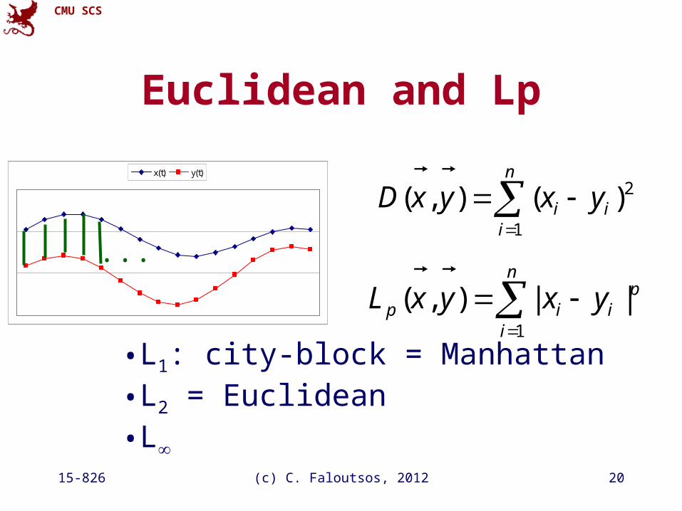
Euclidean and Lp
n
iii yxyxD
1
2)(),(x(t) y(t)
...
n
i
piip yxyxL
1
||),(
•L1: city-block = Manhattan
•L2 = Euclidean
•L
CMU SCS
15-826 (c) C. Faloutsos, 2012 21
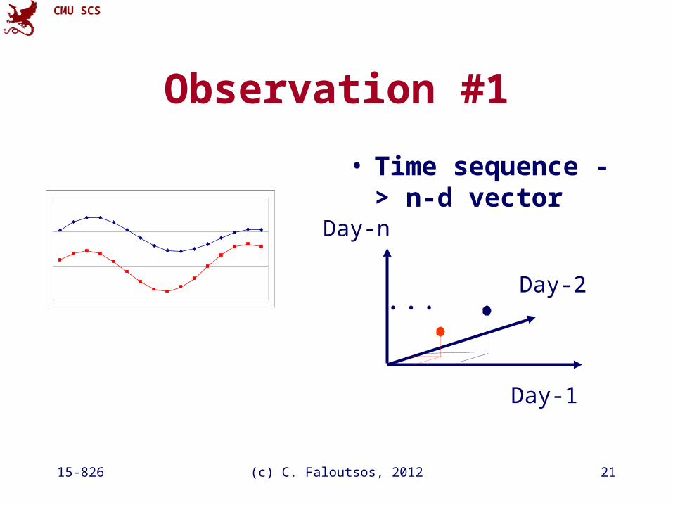
Observation #1
• Time sequence -> n-d vector
...
Day-1
Day-2
Day-n
CMU SCS
15-826 (c) C. Faloutsos, 2012 22
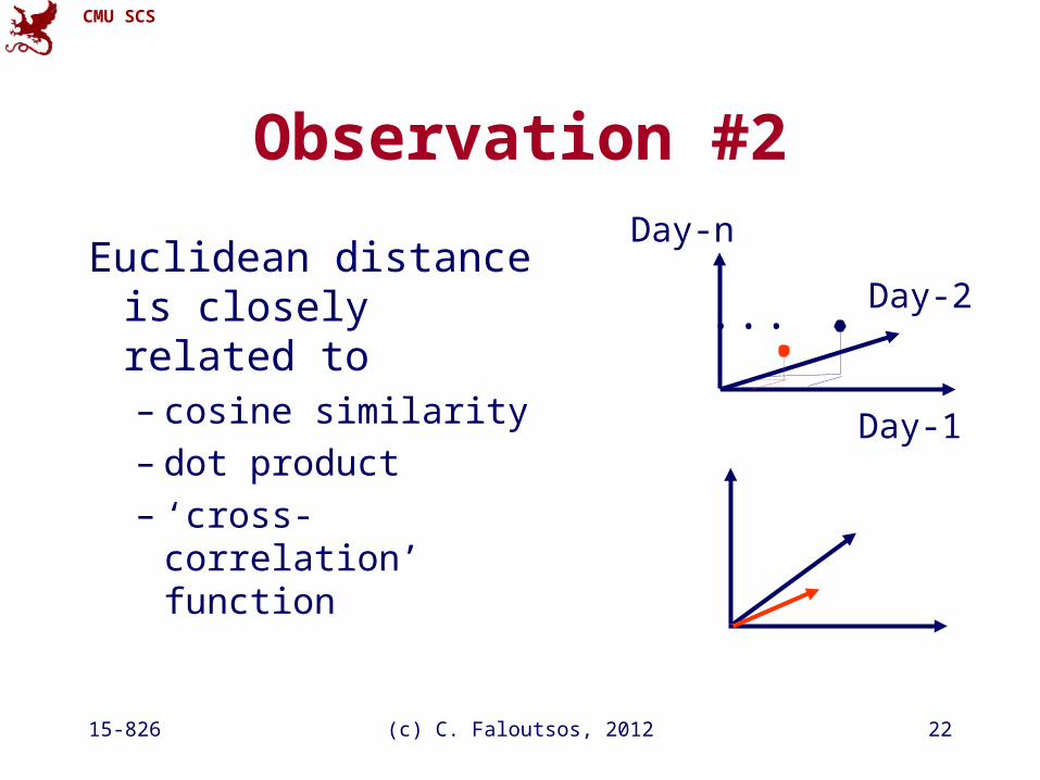
Observation #2
Euclidean distance is closely related to – cosine similarity– dot product– ‘cross-correlation’
function
...
Day-1
Day-2
Day-n
CMU SCS
15-826 (c) C. Faloutsos, 2012 23
Time Warping
• allow accelerations - decelerations– (with or w/o penalty)
• THEN compute the (Euclidean) distance (+ penalty)
• related to the string-editing distance
CMU SCS
15-826 (c) C. Faloutsos, 2012 24
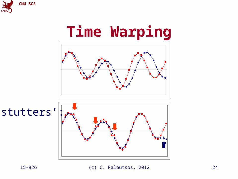
Time Warping
‘stutters’:
CMU SCS
15-826 (c) C. Faloutsos, 2012 25
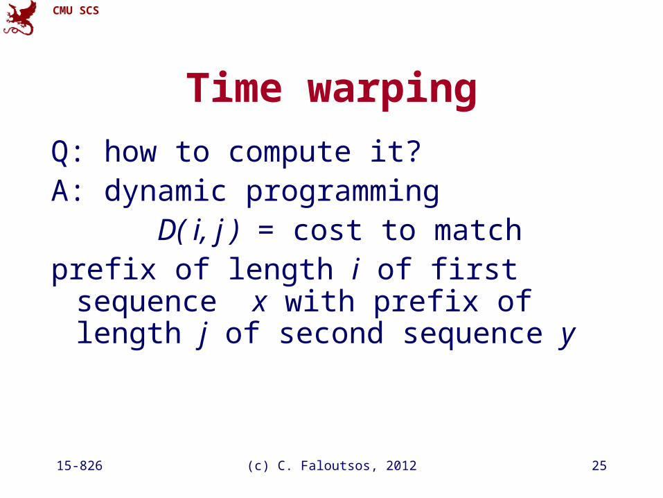
Time warping
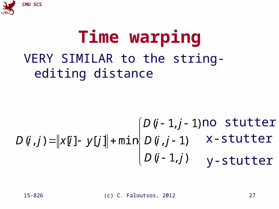
Q: how to compute it?A: dynamic programming D( i, j ) = cost to match prefix of length i of first sequence x with prefix
of length j of second sequence y
CMU SCS
15-826 (c) C. Faloutsos, 2012 26
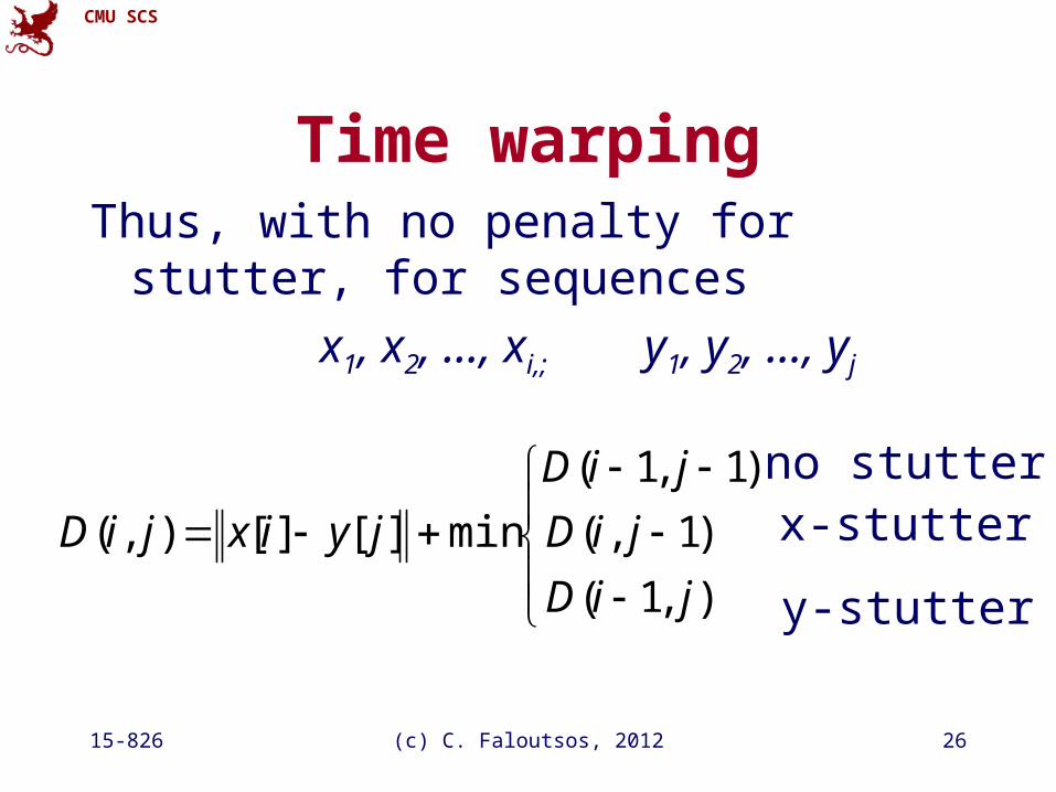
Thus, with no penalty for stutter, for sequences
x1, x2, …, xi,; y1, y2, …, yj
),1(
)1,(
)1,1(
min][][),(
jiD
jiD
jiD
jyixjiD x-stutter
y-stutter
no stutter
Time warping
CMU SCS
15-826 (c) C. Faloutsos, 2012 27
VERY SIMILAR to the string-editing distance
),1(
)1,(
)1,1(
min][][),(
jiD
jiD
jiD
jyixjiD x-stutter
y-stutter
no stutter
Time warping
CMU SCS
15-826 (c) C. Faloutsos, 2012 28
Time warping
• Complexity: O(M*N) - quadratic on the length of the strings
• Many variations (penalty for stutters; limit on the number/percentage of stutters; …)
• popular in voice processing [Rabiner + Juang]
CMU SCS
15-826 (c) C. Faloutsos, 2012 29
Other Distance functions
• piece-wise linear/flat approx.; compare pieces [Keogh+01] [Faloutsos+97]
• ‘cepstrum’ (for voice [Rabiner+Juang])– do DFT; take log of amplitude; do DFT again!
• Allow for small gaps [Agrawal+95]
See tutorial by [Gunopulos + Das, SIGMOD01]
CMU SCS
15-826 (c) C. Faloutsos, 2012 30
Other Distance functions
• In [Keogh+, KDD’04]: parameter-free, MDL based
CMU SCS
15-826 (c) C. Faloutsos, 2012 31
Conclusions
Prevailing distances: – Euclidean and – time-warping
CMU SCS
15-826 (c) C. Faloutsos, 2012 32
Outline
• Motivation
• Similarity search and distance functions
• Linear Forecasting
• Bursty traffic - fractals and multifractals
• Non-linear forecasting
• Conclusions
CMU SCS
15-826 (c) C. Faloutsos, 2012 33
Linear Forecasting

CMU SCS
15-826 (c) C. Faloutsos, 2012 34
Forecasting
"Prediction is very difficult, especially about the future." - Nils Bohr
http://www.hfac.uh.edu/MediaFutures/thoughts.html
CMU SCS
15-826 (c) C. Faloutsos, 2012 35
Outline
• Motivation
• ...
• Linear Forecasting– Auto-regression: Least Squares; RLS– Co-evolving time sequences– Examples– Conclusions
CMU SCS
15-826 (c) C. Faloutsos, 2012 36
Reference
[Yi+00] Byoung-Kee Yi et al.: Online Data Mining for Co-Evolving Time Sequences, ICDE 2000. (Describes MUSCLES and Recursive Least Squares)
CMU SCS
15-826 (c) C. Faloutsos, 2012 37
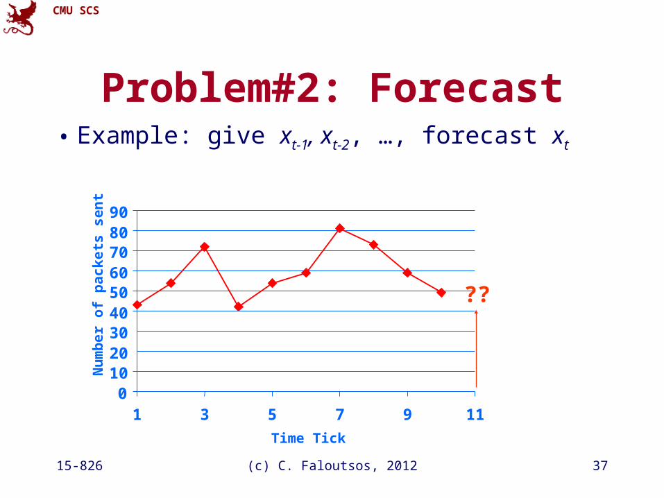
Problem#2: Forecast• Example: give xt-1, xt-2, …, forecast xt
0102030405060708090
1 3 5 7 9 11
Time Tick
Nu
mb
er o
f p
ack
ets
sen
t
??
CMU SCS
15-826 (c) C. Faloutsos, 2012 38
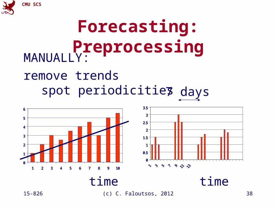
Forecasting: PreprocessingMANUALLY:
remove trends spot periodicities
0
1
2
3
4
5
6
1 2 3 4 5 6 7 8 9 10
0
0.5
1
1.5
2
2.5
3
3.5
1 3 5 7 9 11 13
timetime
7 days
CMU SCS
15-826 (c) C. Faloutsos, 2012 39
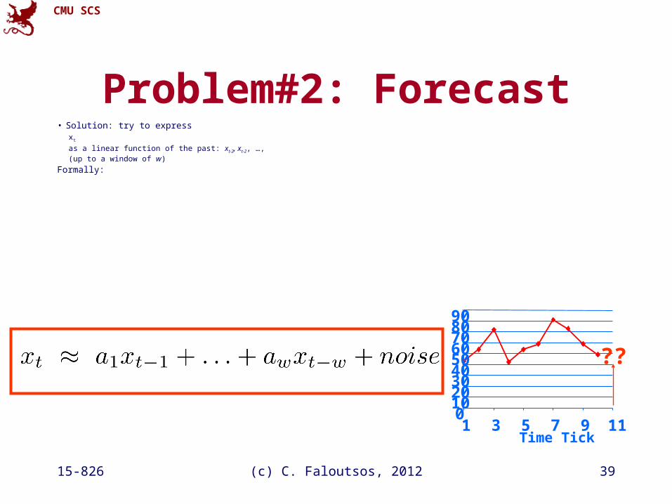
Problem#2: Forecast• Solution: try to express
xt
as a linear function of the past: xt-2, xt-2, …, (up to a window of w)
Formally:
0102030405060708090
1 3 5 7 9 11Time Tick
??
CMU SCS
15-826 (c) C. Faloutsos, 2012 40
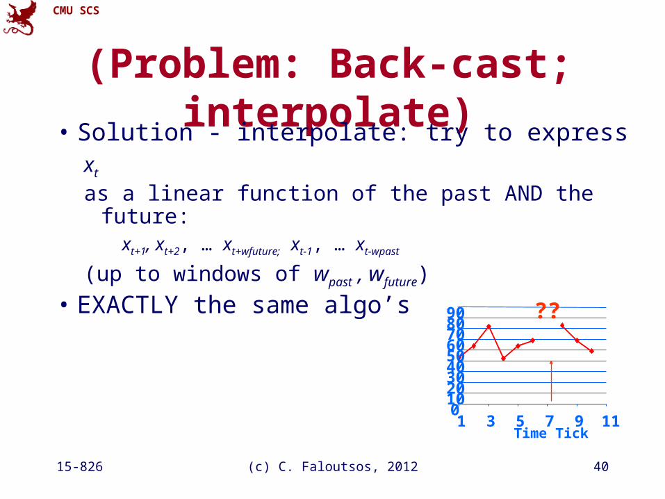
(Problem: Back-cast; interpolate)• Solution - interpolate: try to express
xt
as a linear function of the past AND the future: xt+1, xt+2, … xt+wfuture; xt-1, … xt-wpast
(up to windows of wpast , wfuture)
• EXACTLY the same algo’s
0102030405060708090
1 3 5 7 9 11Time Tick
??
CMU SCS
15-826 (c) C. Faloutsos, 2012 41
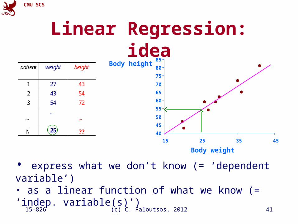
Linear Regression: idea
40
45
50
55
60
65
70
75
80
85
15 25 35 45
Body weight
patient weight height
1 27 43
2 43 54
3 54 72
……
…
N 25 ??
• express what we don’t know (= ‘dependent variable’)• as a linear function of what we know (= ‘indep. variable(s)’)
Body height
CMU SCS
15-826 (c) C. Faloutsos, 2012 42
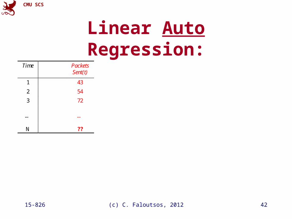
Linear Auto Regression:Time Packets
Sent (t-1)PacketsSent(t)
1 - 43
2 43 54
3 54 72
……
…
N 25 ??
CMU SCS
15-826 (c) C. Faloutsos, 2012 43
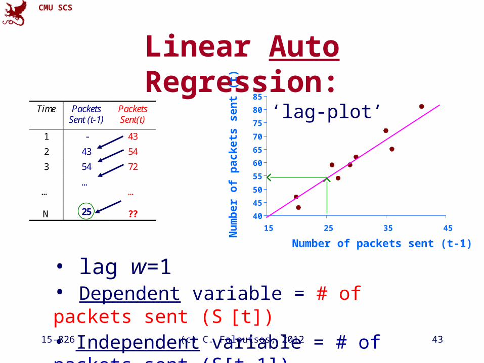
Linear Auto Regression:
40
45
50
55
60
65
70
75
80
85
15 25 35 45
Number of packets sent (t-1)N
um
ber
of
pac
ket
s se
nt
(t)
Time PacketsSent (t-1)
PacketsSent(t)
1 - 43
2 43 54
3 54 72
……
…
N 25 ??
• lag w=1• Dependent variable = # of packets sent (S [t])• Independent variable = # of packets sent (S[t-1])
‘lag-plot’
CMU SCS
15-826 (c) C. Faloutsos, 2012 44
Outline
• Motivation
• ...
• Linear Forecasting– Auto-regression: Least Squares; RLS– Co-evolving time sequences– Examples– Conclusions
CMU SCS
15-826 (c) C. Faloutsos, 2012 45
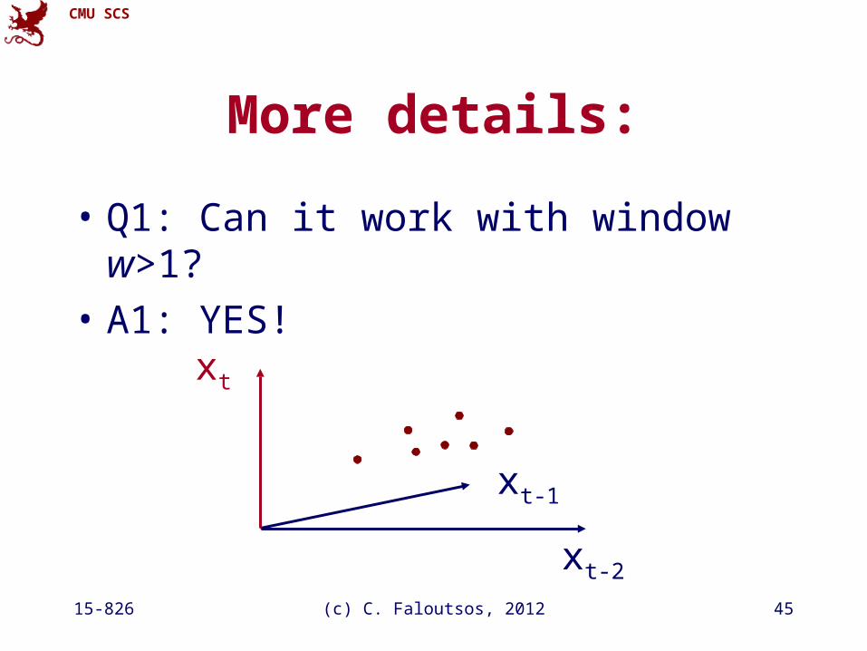
More details:
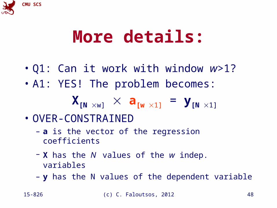
• Q1: Can it work with window w>1?
• A1: YES!
xt-2
xt
xt-1
CMU SCS
15-826 (c) C. Faloutsos, 2012 46
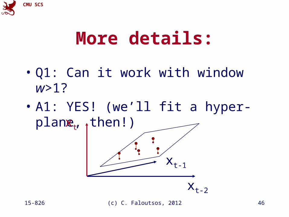
More details:
• Q1: Can it work with window w>1?
• A1: YES! (we’ll fit a hyper-plane, then!)
xt-2
xt
xt-1
CMU SCS
15-826 (c) C. Faloutsos, 2012 47
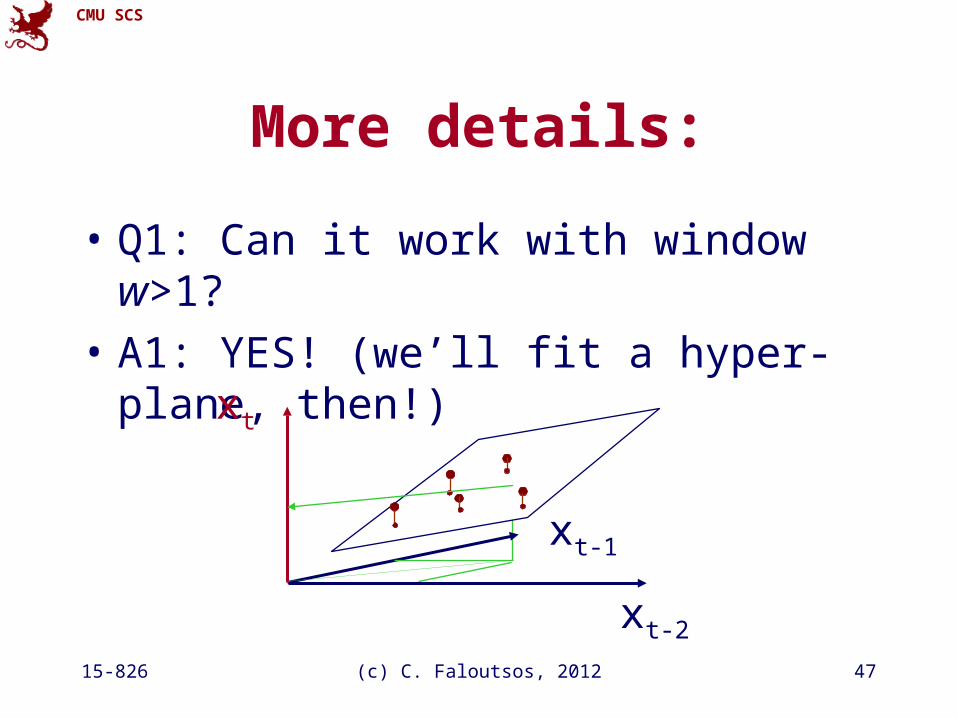
More details:
• Q1: Can it work with window w>1?
• A1: YES! (we’ll fit a hyper-plane, then!)
xt-2
xt-1
xt
CMU SCS
15-826 (c) C. Faloutsos, 2012 48
More details:
• Q1: Can it work with window w>1?
• A1: YES! The problem becomes:
X[N w] a[w 1] = y[N 1]
• OVER-CONSTRAINED– a is the vector of the regression coefficients
– X has the N values of the w indep. variables
– y has the N values of the dependent variable
CMU SCS
15-826 (c) C. Faloutsos, 2012 49
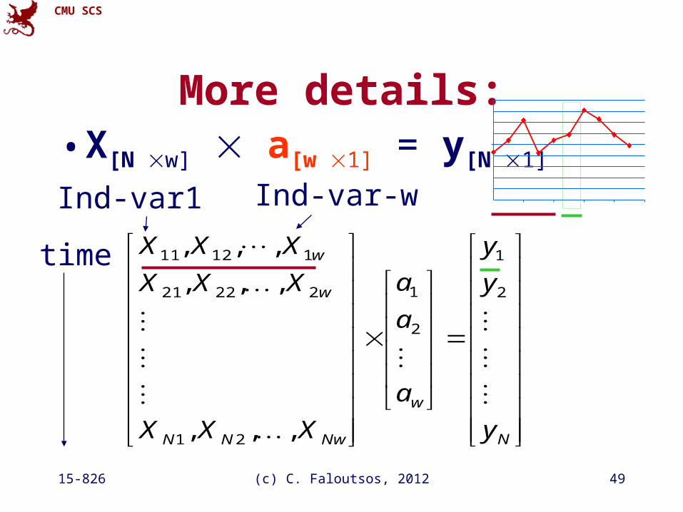
More details:• X[N w] a[w 1] = y[N 1]
N
w
NwNN
w
w
y
y
y
a
a
a
XXX
XXX
XXX
2
1
2
1
21
22221
11211
,,,
,,,
,,,
Ind-var1 Ind-var-w
time
CMU SCS
15-826 (c) C. Faloutsos, 2012 50
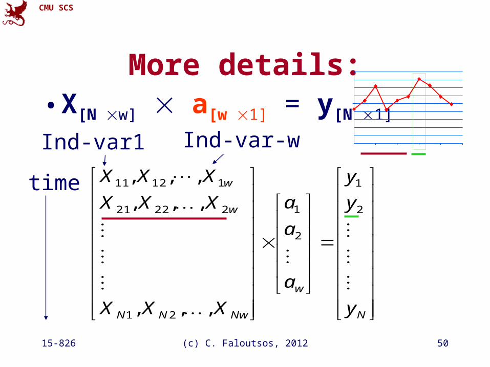
More details:• X[N w] a[w 1] = y[N 1]
N
w
NwNN
w
w
y
y
y
a
a
a
XXX
XXX
XXX
2
1
2
1
21
22221
11211
,,,
,,,
,,,
Ind-var1 Ind-var-w
time
CMU SCS
15-826 (c) C. Faloutsos, 2012 51
More details
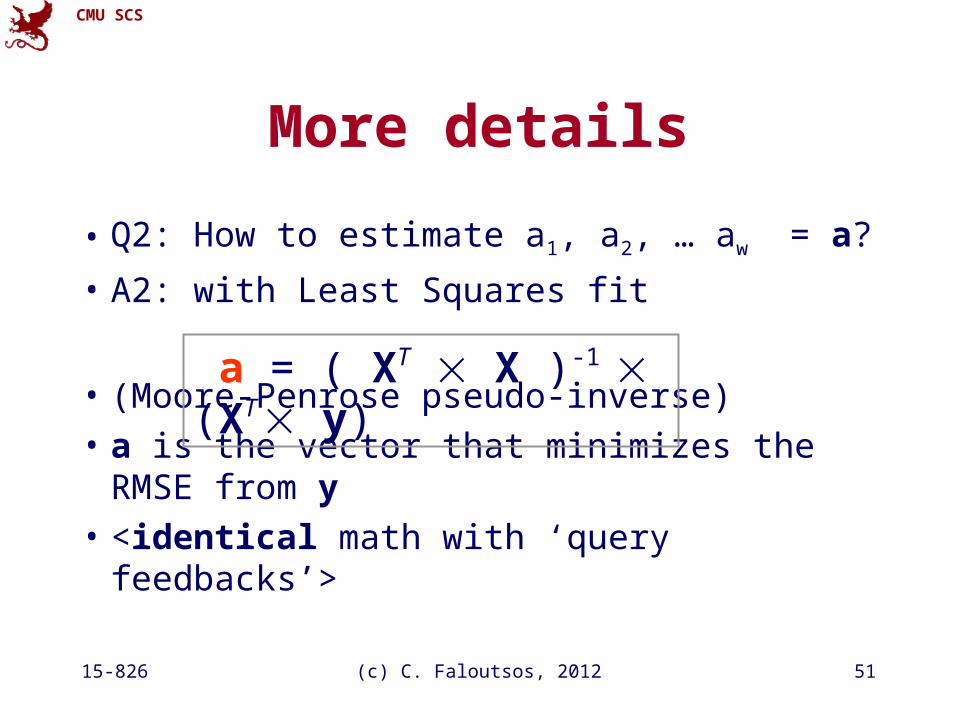
• Q2: How to estimate a1, a2, … aw = a?
• A2: with Least Squares fit
• (Moore-Penrose pseudo-inverse)
• a is the vector that minimizes the RMSE from y
• <identical math with ‘query feedbacks’>
a = ( XT X )-1 (XT y)

CMU SCS
15-826 (c) C. Faloutsos, 2012 52
More details• Straightforward solution:
• Observations:– Sample matrix X grows over time
– needs matrix inversion
– O(Nw2) computation
– O(Nw) storage
a = ( XT X )-1 (XT y)
a : Regression Coeff. VectorX : Sample Matrix
XN:
w
N
CMU SCS
15-826 (c) C. Faloutsos, 2012 53
Even more details
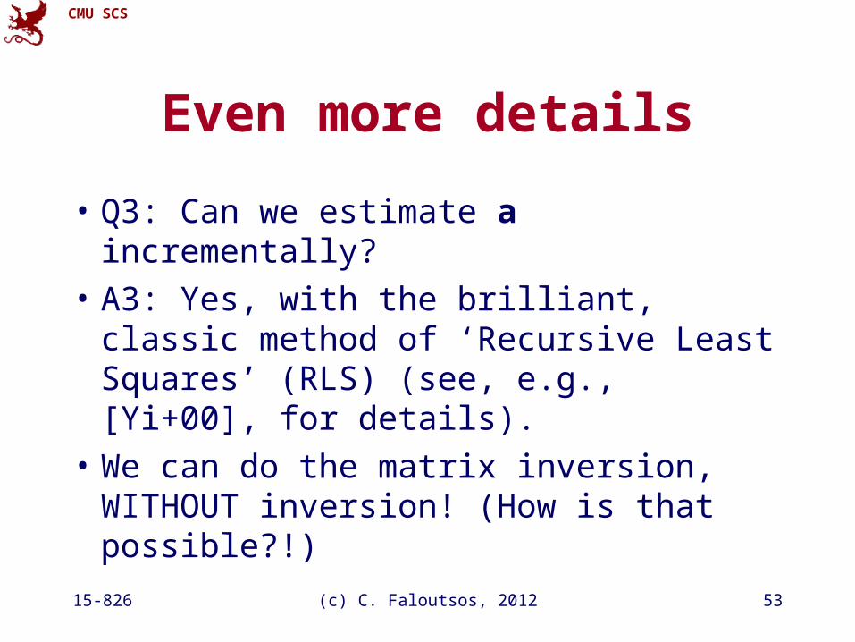
• Q3: Can we estimate a incrementally?
• A3: Yes, with the brilliant, classic method of ‘Recursive Least Squares’ (RLS) (see, e.g., [Yi+00], for details).
• We can do the matrix inversion, WITHOUT inversion! (How is that possible?!)
CMU SCS
15-826 (c) C. Faloutsos, 2012 54
Even more details
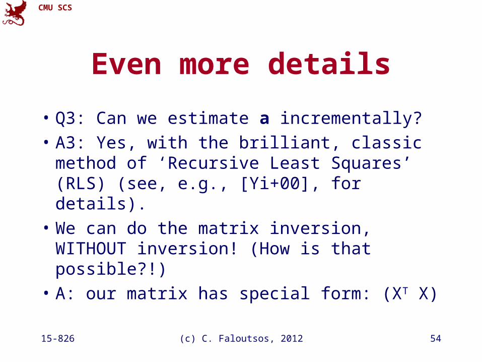
• Q3: Can we estimate a incrementally?
• A3: Yes, with the brilliant, classic method of ‘Recursive Least Squares’ (RLS) (see, e.g., [Yi+00], for details).
• We can do the matrix inversion, WITHOUT inversion! (How is that possible?!)
• A: our matrix has special form: (XT X)
CMU SCS
15-826 (c) C. Faloutsos, 2012 55
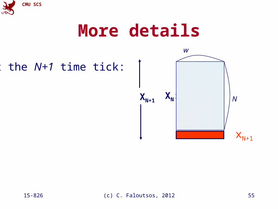
More details
XN:
w
NXN+1
At the N+1 time tick:
xN+1
CMU SCS
15-826 (c) C. Faloutsos, 2012 56
More details
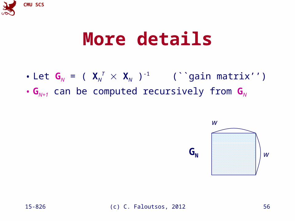
• Let GN = ( XNT XN )-1 (``gain matrix’’)
• GN+1 can be computed recursively from GN
GN
w
w
CMU SCS
15-826 (c) C. Faloutsos, 2012 57
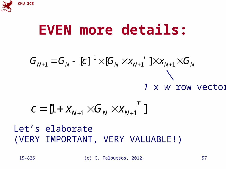
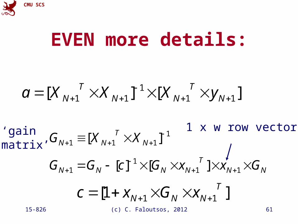
EVEN more details:
NNT
NNNN GxxGcGG
111
1 ][][
]1[ 11T
NNN xGxc
1 x w row vector
Let’s elaborate (VERY IMPORTANT, VERY VALUABLE!)
CMU SCS
15-826 (c) C. Faloutsos, 2012 58
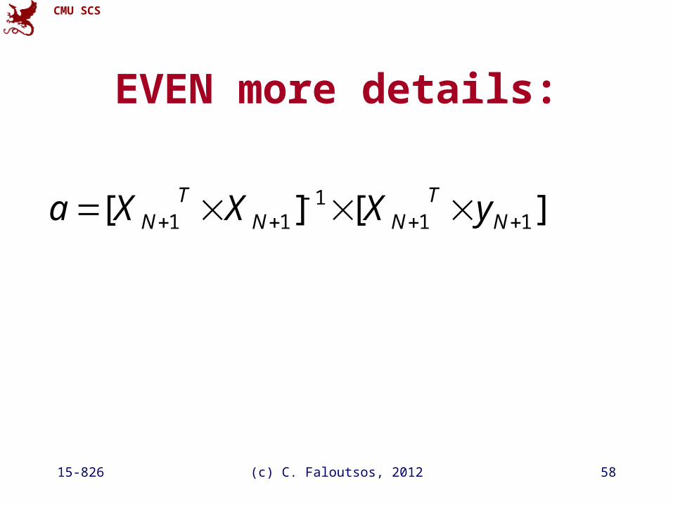
EVEN more details:
][][ 111
11
NT
NNT
N yXXXa
CMU SCS
15-826 (c) C. Faloutsos, 2012 59
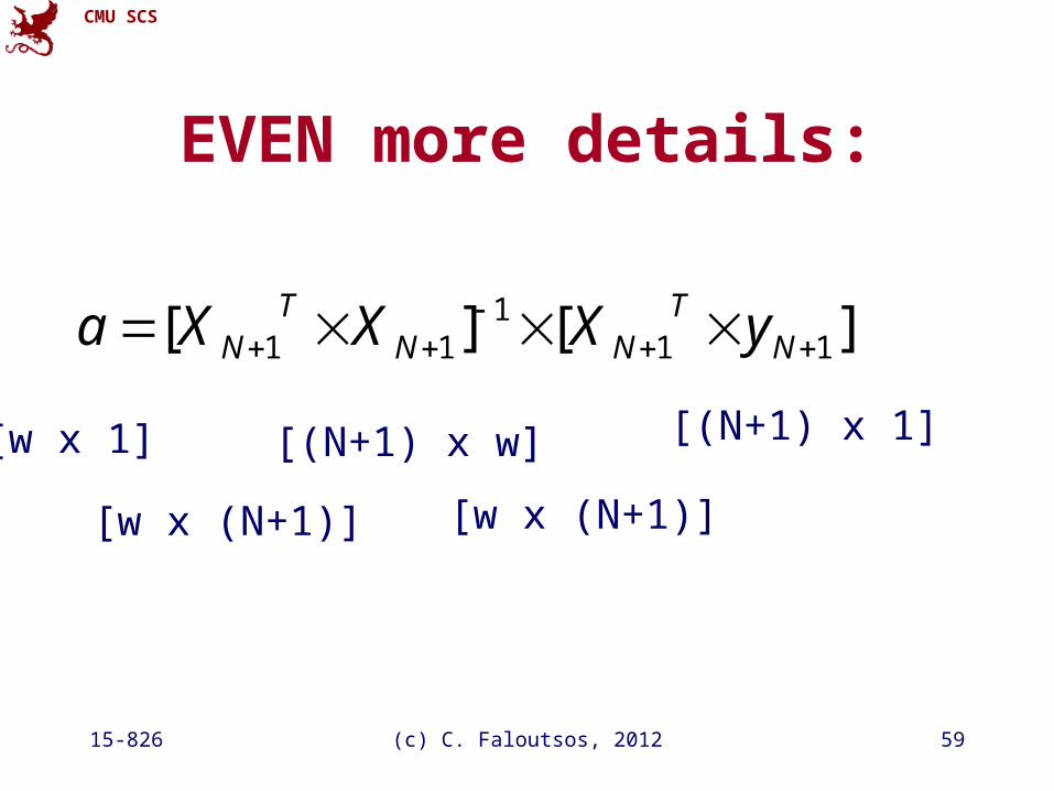
EVEN more details:
][][ 111
11
NT
NNT
N yXXXa
[w x 1]
[w x (N+1)]
[(N+1) x w]
[w x (N+1)]
[(N+1) x 1]
CMU SCS
15-826 (c) C. Faloutsos, 2012 60
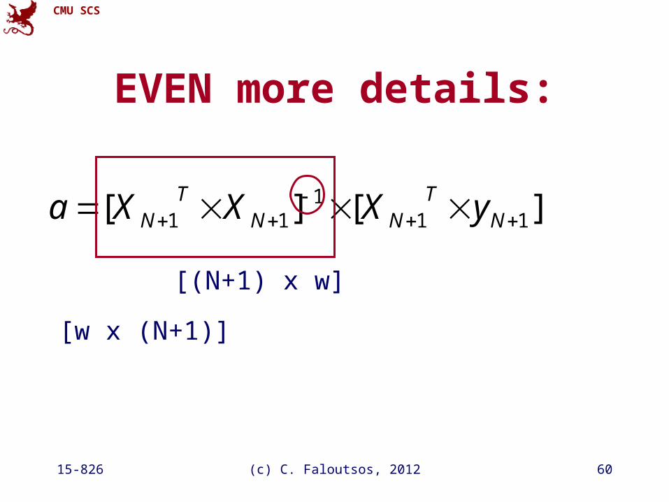
EVEN more details:
][][ 111
11
NT
NNT
N yXXXa
[w x (N+1)]
[(N+1) x w]
CMU SCS
15-826 (c) C. Faloutsos, 2012 61
EVEN more details:
NNT
NNNN GxxGcGG
111
1 ][][
]1[ 11T
NNN xGxc
][][ 111
11
NT
NNT
N yXXXa
1111 ][
NT
NN XXG1 x w row vector‘gain
matrix’
CMU SCS
15-826 (c) C. Faloutsos, 2012 62
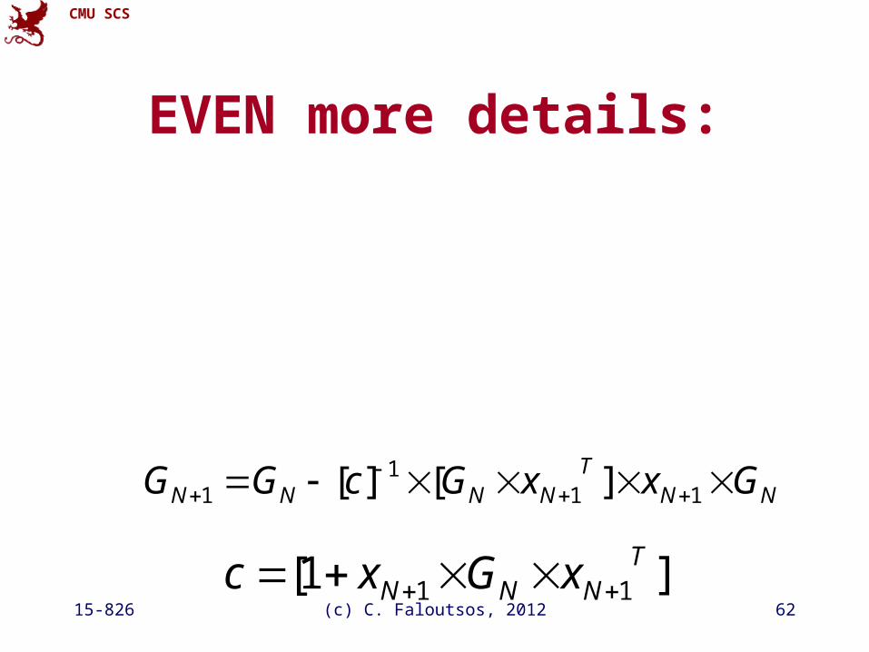
EVEN more details:
NNT
NNNN GxxGcGG
111
1 ][][
]1[ 11T
NNN xGxc
CMU SCS
15-826 (c) C. Faloutsos, 2012 63
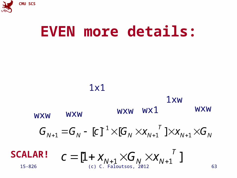
EVEN more details:
NNT
NNNN GxxGcGG
111
1 ][][
]1[ 11T
NNN xGxc
wxw wxw wxw wx11xw
wxw
1x1
SCALAR!

CMU SCS
15-826 (c) C. Faloutsos, 2012 64
Altogether:
NNT
NNNN GxxGcGG
111
1 ][][
]1[ 11T
NNN xGxc
][][ 111
11
NT
NNT
N yXXXa
1111 ][
NT
NN XXG
CMU SCS
15-826 (c) C. Faloutsos, 2012 65
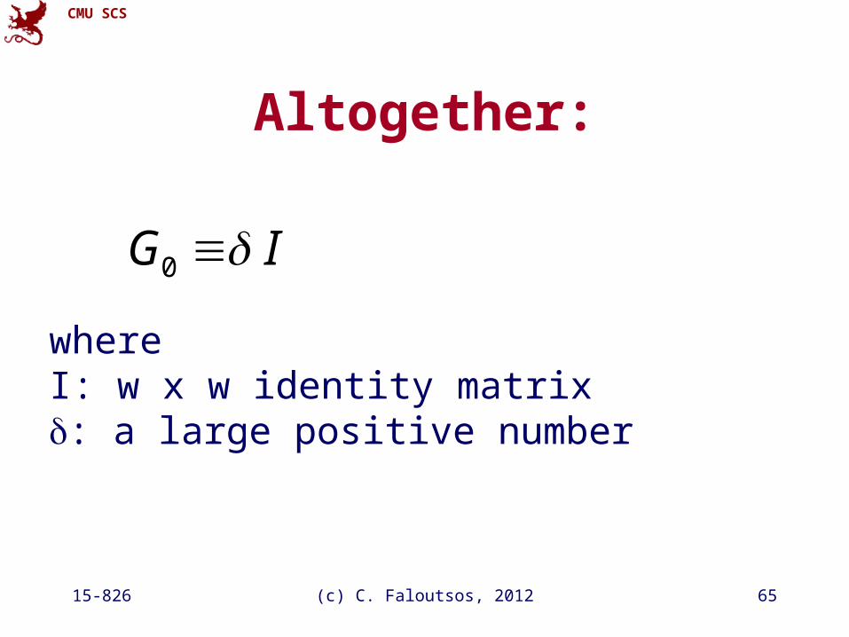
Altogether:
IG 0
where I: w x w identity matrix: a large positive number
CMU SCS
15-826 (c) C. Faloutsos, 2012 66
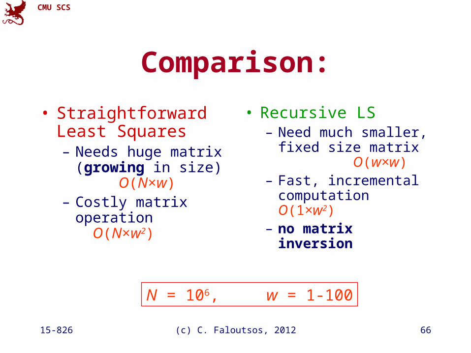
Comparison:
• Straightforward Least Squares– Needs huge matrix
(growing in size) O(N×w)
– Costly matrix operation O(N×w2)
• Recursive LS– Need much smaller,
fixed size matrix O(w×w)
– Fast, incremental computation O(1×w2)
– no matrix inversion
N = 106, w = 1-100
CMU SCS
15-826 (c) C. Faloutsos, 2012 67
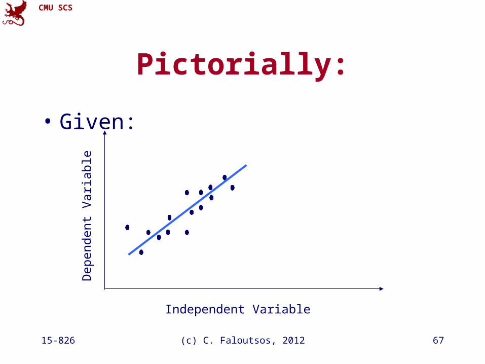
Pictorially:
• Given:
Independent Variable
Dep
ende
nt V
aria
ble

CMU SCS
15-826 (c) C. Faloutsos, 2012 68
Pictorially:
Independent Variable
Dep
ende
nt V
aria
ble
.
new point
CMU SCS
15-826 (c) C. Faloutsos, 2012 69
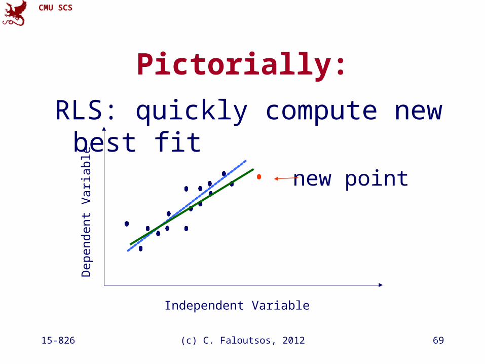
Pictorially:
Independent Variable
Dep
ende
nt V
aria
ble
RLS: quickly compute new best fit
new point
CMU SCS
15-826 (c) C. Faloutsos, 2012 70
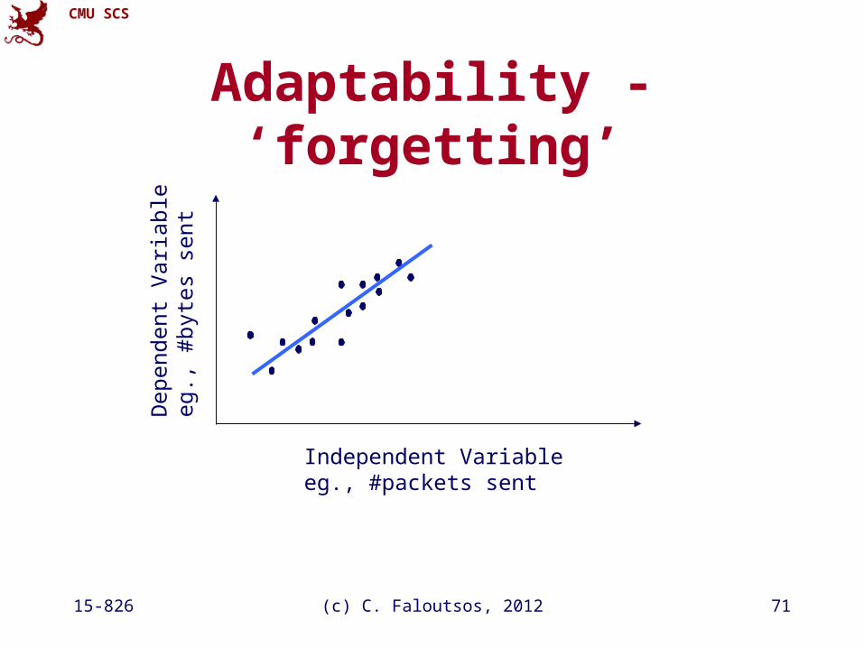
Even more details
• Q4: can we ‘forget’ the older samples?
• A4: Yes - RLS can easily handle that [Yi+00]:
CMU SCS
15-826 (c) C. Faloutsos, 2012 71
Adaptability - ‘forgetting’
Independent Variableeg., #packets sent
Dep
ende
nt V
aria
ble
eg.,
#byt
es s
ent
CMU SCS
15-826 (c) C. Faloutsos, 2012 72
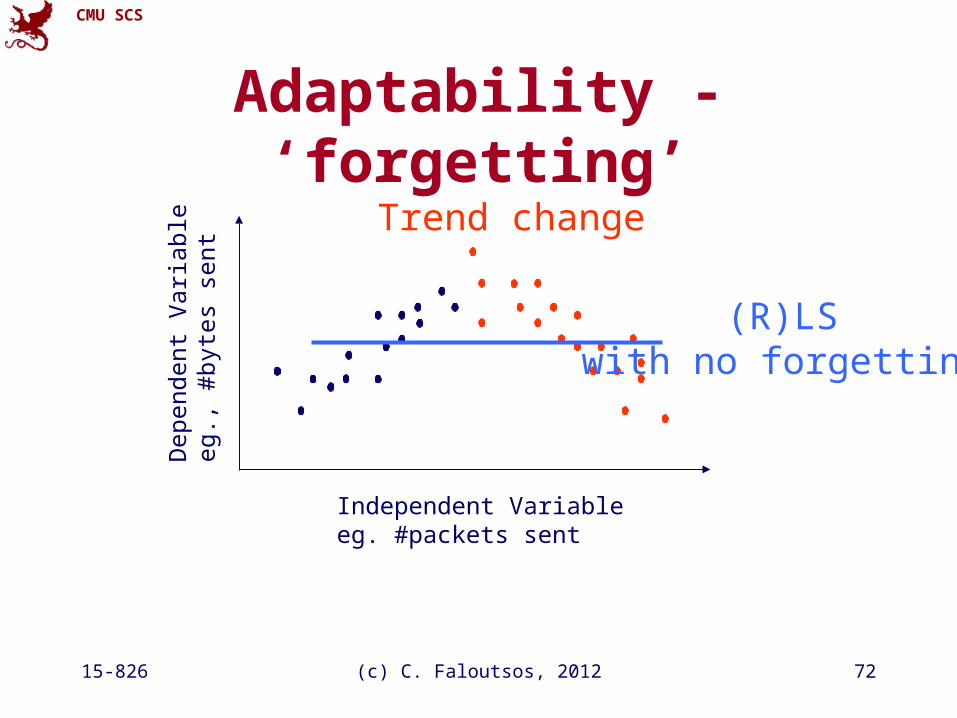
Adaptability - ‘forgetting’
Independent Variableeg. #packets sent
Dep
ende
nt V
aria
ble
eg.,
#byt
es s
ent
Trend change
(R)LSwith no forgetting
CMU SCS
15-826 (c) C. Faloutsos, 2012 73
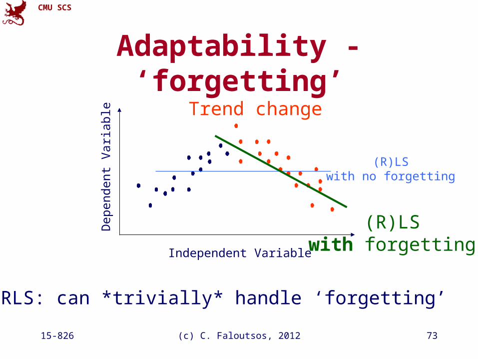
Adaptability - ‘forgetting’
Independent Variable
Dep
ende
nt V
aria
ble
Trend change
(R)LSwith no forgetting
(R)LSwith forgetting
• RLS: can *trivially* handle ‘forgetting’
CMU SCS
15-826 (c) C. Faloutsos, 2012 74
How to choose ‘w’?
• goal: capture arbitrary periodicities
• with NO human intervention
• on a semi-infinite stream
SKIP
CMU SCS
15-826 (c) C. Faloutsos, 2012 75
Reference
[Papadimitriou+ vldb2003] Spiros Papadimitriou, Anthony Brockwell and Christos Faloutsos Adaptive, Hands-Off Stream Mining VLDB 2003, Berlin, Germany, Sept. 2003
SKIP
CMU SCS
15-826 (c) C. Faloutsos, 2012 76
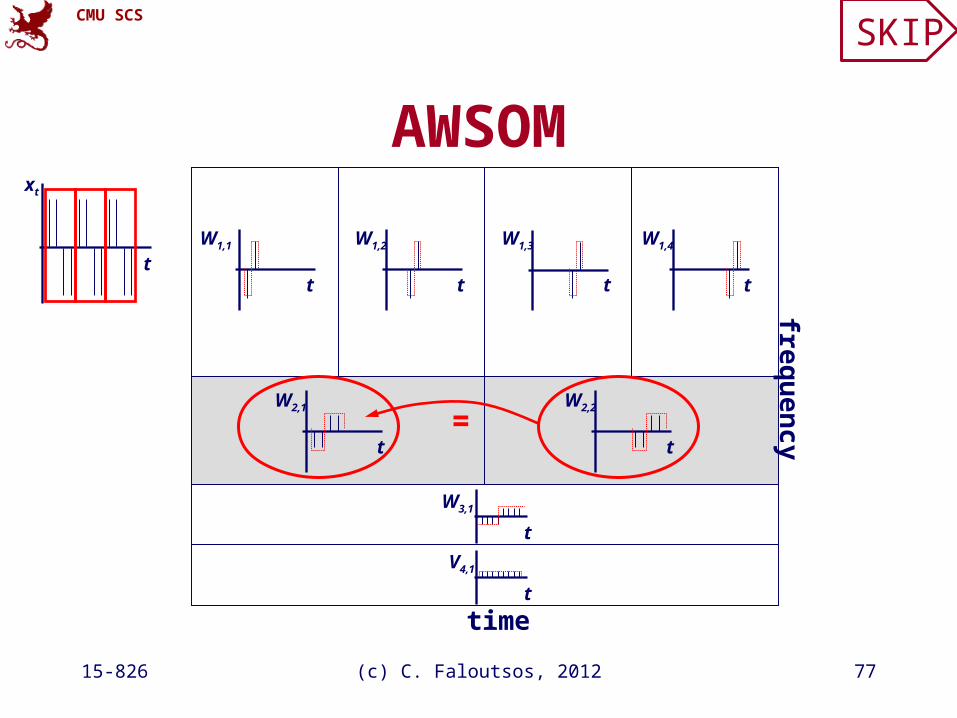
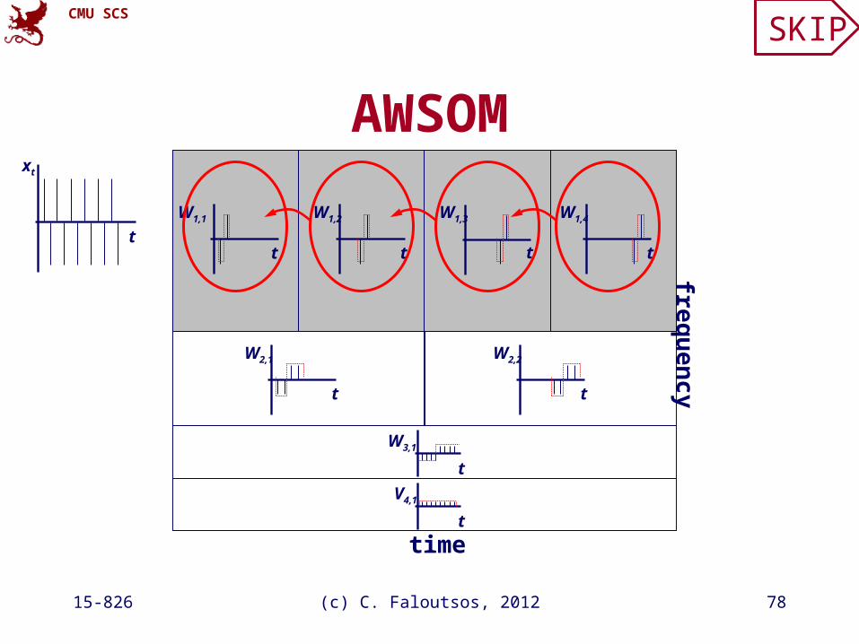
Answer:
• ‘AWSOM’ (Arbitrary Window Stream fOrecasting Method) [Papadimitriou+, vldb2003]
• idea: do AR on each wavelet level
• in detail:
SKIP
CMU SCS
15-826 (c) C. Faloutsos, 2012 77
AWSOMxt
tt
W1,1
t
W1,2
t
W1,3
t
W1,4
t
W2,1
t
W2,2
t
W3,1
t
V4,1
time
frequ
ency=
SKIP
CMU SCS
15-826 (c) C. Faloutsos, 2012 78
AWSOMxt
tt
W1,1
t
W1,2
t
W1,3
t
W1,4
t
W2,1
t
W2,2
t
W3,1
t
V4,1
time
frequ
ency
SKIP
CMU SCS
15-826 (c) C. Faloutsos, 2012 79
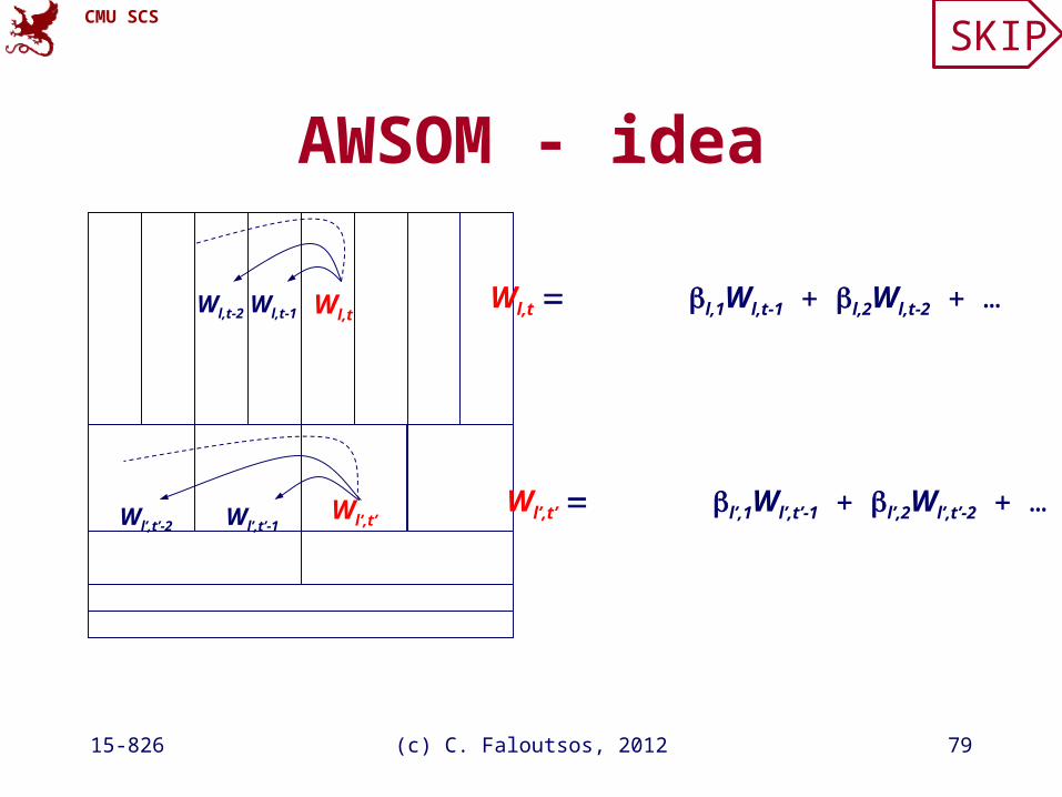
AWSOM - idea
Wl,tWl,t-1Wl,t-2Wl,t l,1Wl,t-1 l,2Wl,t-2 …
Wl’,t’-1Wl’,t’-2Wl’,t’
Wl’,t’ l’,1Wl’,t’-1 l’,2Wl’,t’-2 …
SKIP
CMU SCS
15-826 (c) C. Faloutsos, 2012 80
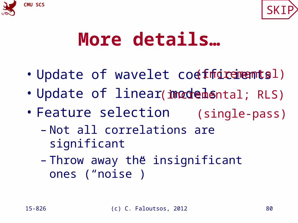
More details…
• Update of wavelet coefficients
• Update of linear models
• Feature selection– Not all correlations are significant– Throw away the insignificant ones (“noise”)
(incremental)
(incremental; RLS)
(single-pass)
SKIP
CMU SCS
15-826 (c) C. Faloutsos, 2012 81
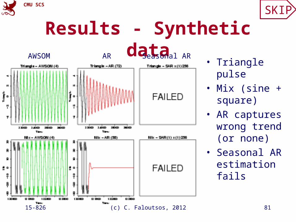
Results - Synthetic data• Triangle pulse
• Mix (sine + square)
• AR captures wrong trend (or none)
• Seasonal AR estimation fails
AWSOM AR Seasonal AR
SKIP
CMU SCS
15-826 (c) C. Faloutsos, 2012 82
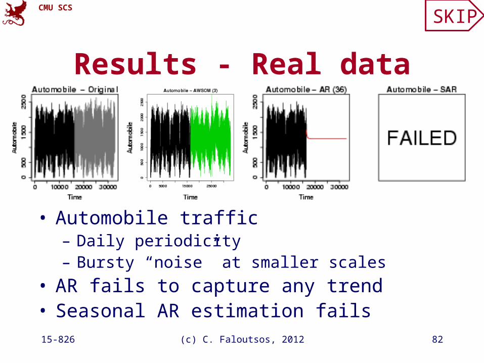
Results - Real data
• Automobile traffic– Daily periodicity– Bursty “noise” at smaller scales
• AR fails to capture any trend• Seasonal AR estimation fails
SKIP
CMU SCS
15-826 (c) C. Faloutsos, 2012 83
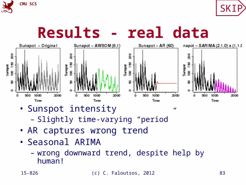
Results - real data
• Sunspot intensity– Slightly time-varying “period”
• AR captures wrong trend• Seasonal ARIMA
– wrong downward trend, despite help by human!
SKIP

CMU SCS
15-826 (c) C. Faloutsos, 2012 84
Complexity
• Model update
Space: OlgN + mk2 OlgNTime: Ok2 O1
• Where– N: number of points (so far)– k: number of regression coefficients; fixed– m: number of linear models; OlgN
SKIP
CMU SCS
15-826 (c) C. Faloutsos, 2012 85
Outline
• Motivation
• ...
• Linear Forecasting– Auto-regression: Least Squares; RLS– Co-evolving time sequences– Examples– Conclusions
CMU SCS
15-826 (c) C. Faloutsos, 2012 86
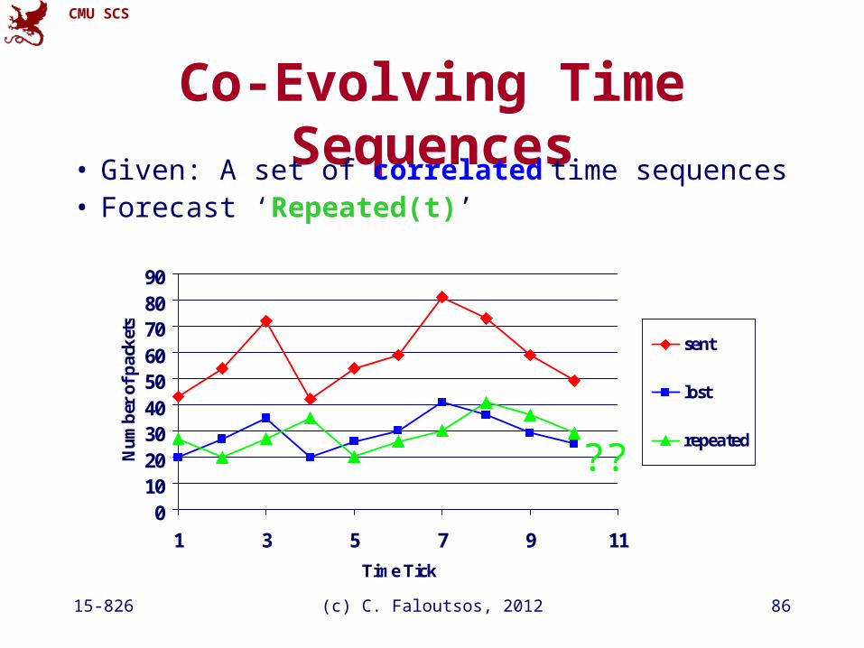
Co-Evolving Time Sequences• Given: A set of correlated time sequences• Forecast ‘Repeated(t)’
0102030405060708090
1 3 5 7 9 11
Time Tick
Nu
mb
er o
f p
ack
ets
sent
lost
repeated
??

CMU SCS
15-826 (c) C. Faloutsos, 2012 87
Solution:
Q: what should we do?
CMU SCS
15-826 (c) C. Faloutsos, 2012 88
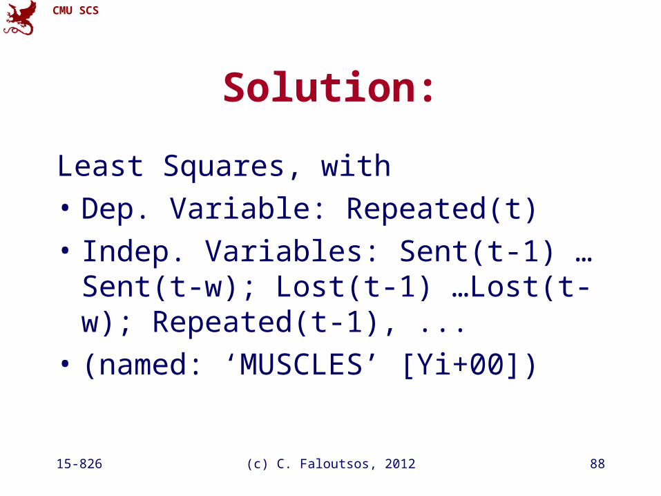
Solution:
Least Squares, with
• Dep. Variable: Repeated(t)
• Indep. Variables: Sent(t-1) … Sent(t-w); Lost(t-1) …Lost(t-w); Repeated(t-1), ...
• (named: ‘MUSCLES’ [Yi+00])
CMU SCS
15-826 (c) C. Faloutsos, 2012 89
Forecasting - Outline
• Auto-regression
• Least Squares; recursive least squares
• Co-evolving time sequences
• Examples
• Conclusions
CMU SCS
15-826 (c) C. Faloutsos, 2012 90
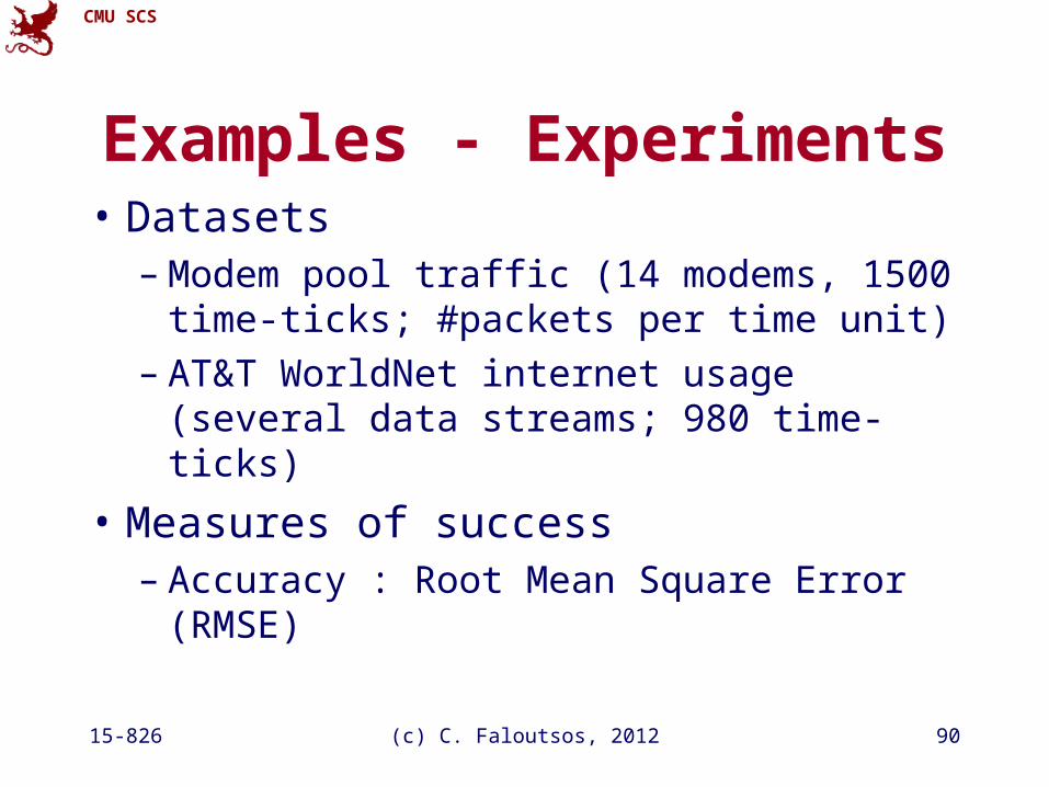
Examples - Experiments• Datasets
– Modem pool traffic (14 modems, 1500 time-ticks; #packets per time unit)
– AT&T WorldNet internet usage (several data streams; 980 time-ticks)
• Measures of success– Accuracy : Root Mean Square Error (RMSE)
CMU SCS
15-826 (c) C. Faloutsos, 2012 91
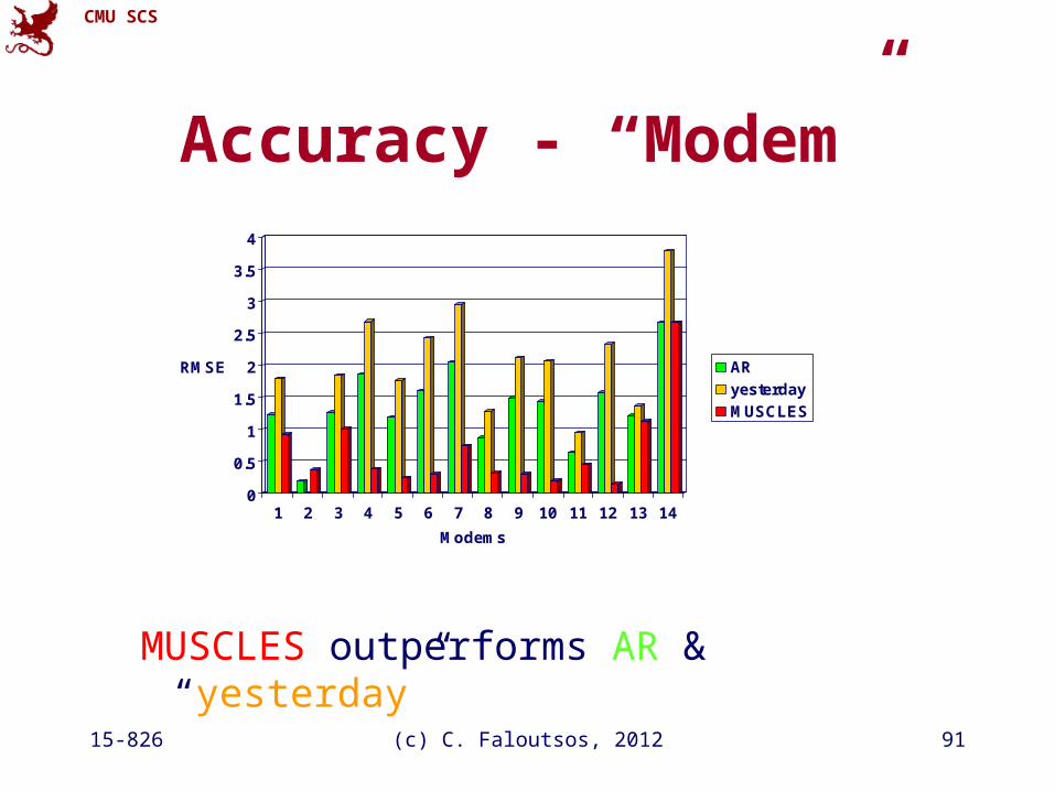
Accuracy - “Modem”
MUSCLES outperforms AR & “yesterday”
0
0.5
1
1.5
2
2.5
3
3.5
4
RMSE
1 2 3 4 5 6 7 8 9 10 11 12 13 14
Modems
AR
yesterday
MUSCLES
CMU SCS
15-826 (c) C. Faloutsos, 2012 92
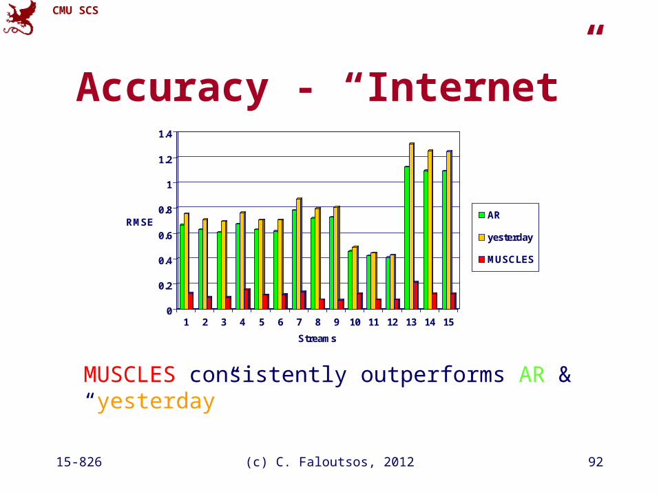
Accuracy - “Internet”
0
0.2
0.4
0.6
0.8
1
1.2
1.4
RMSE
1 2 3 4 5 6 7 8 9 10 11 12 13 14 15
Streams
AR
yesterday
MUSCLES
MUSCLES consistently outperforms AR & “yesterday”
CMU SCS
15-826 (c) C. Faloutsos, 2012 93
Linear forecasting - Outline
• Auto-regression
• Least Squares; recursive least squares
• Co-evolving time sequences
• Examples
• Conclusions
CMU SCS
15-826 (c) C. Faloutsos, 2012 94
Conclusions - Practitioner’s guide
• AR(IMA) methodology: prevailing method for linear forecasting
• Brilliant method of Recursive Least Squares for fast, incremental estimation.
• See [Box-Jenkins]
• (AWSOM: no human intervention)
CMU SCS
15-826 (c) C. Faloutsos, 2012 95
Resources: software and urls
• MUSCLES: Prof. Byoung-Kee Yi:http://www.postech.ac.kr/~bkyi/or [email protected]
• free-ware: ‘R’ for stat. analysis (clone of Splus) http://cran.r-project.org/
CMU SCS
15-826 (c) C. Faloutsos, 2012 96
Books
• George E.P. Box and Gwilym M. Jenkins and Gregory C. Reinsel, Time Series Analysis: Forecasting and Control, Prentice Hall, 1994 (the classic book on ARIMA, 3rd ed.)
• Brockwell, P. J. and R. A. Davis (1987). Time Series: Theory and Methods. New York, Springer Verlag.
CMU SCS
15-826 (c) C. Faloutsos, 2012 97
Additional Reading
• [Papadimitriou+ vldb2003] Spiros Papadimitriou, Anthony Brockwell and Christos Faloutsos Adaptive, Hands-Off Stream Mining VLDB 2003, Berlin, Germany, Sept. 2003
• [Yi+00] Byoung-Kee Yi et al.: Online Data Mining for Co-Evolving Time Sequences, ICDE 2000. (Describes MUSCLES and Recursive Least Squares)
CMU SCS
15-826 (c) C. Faloutsos, 2012 98
Outline
• Motivation
• Similarity search and distance functions
• Linear Forecasting
• Bursty traffic - fractals and multifractals
• Non-linear forecasting
• Conclusions
CMU SCS
15-826 (c) C. Faloutsos, 2012 99
Bursty Traffic& Multifractals
CMU SCS
15-826 (c) C. Faloutsos, 2012 100
Outline
• Motivation
• ...
• Linear Forecasting
• Bursty traffic - fractals and multifractals– Problem– Main idea (80/20, Hurst exponent)– Results
CMU SCS
15-826 (c) C. Faloutsos, 2012 101
Reference:
[Wang+02] Mengzhi Wang, Tara Madhyastha, Ngai Hang Chang, Spiros Papadimitriou and Christos Faloutsos, Data Mining Meets Performance Evaluation: Fast Algorithms for Modeling Bursty Traffic, ICDE 2002, San Jose, CA, 2/26/2002 - 3/1/2002.
Full thesis: CMU-CS-05-185Performance Modeling of Storage Devices using Machine Learning Mengzhi Wang, Ph.D. ThesisAbstract, .ps.gz, .pdf
CMU SCS
15-826 (c) C. Faloutsos, 2012 102
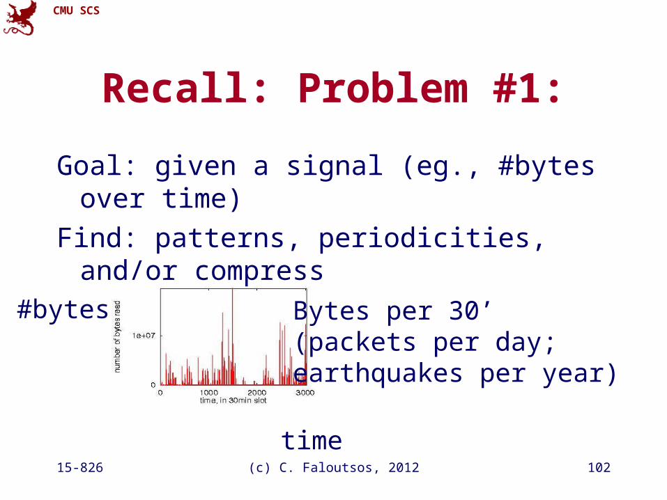
Recall: Problem #1:
Goal: given a signal (eg., #bytes over time)
Find: patterns, periodicities, and/or compress
time
#bytes Bytes per 30’(packets per day;earthquakes per year)
CMU SCS
15-826 (c) C. Faloutsos, 2012 103
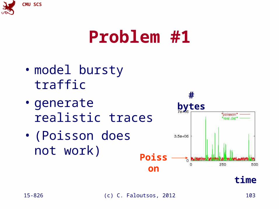
Problem #1
• model bursty traffic
• generate realistic traces
• (Poisson does not work)
time
# bytes
Poisson
CMU SCS
15-826 (c) C. Faloutsos, 2012 104
Motivation
• predict queue length distributions (e.g., to give probabilistic guarantees)
• “learn” traffic, for buffering, prefetching, ‘active disks’, web servers
CMU SCS
15-826 (c) C. Faloutsos, 2012 105
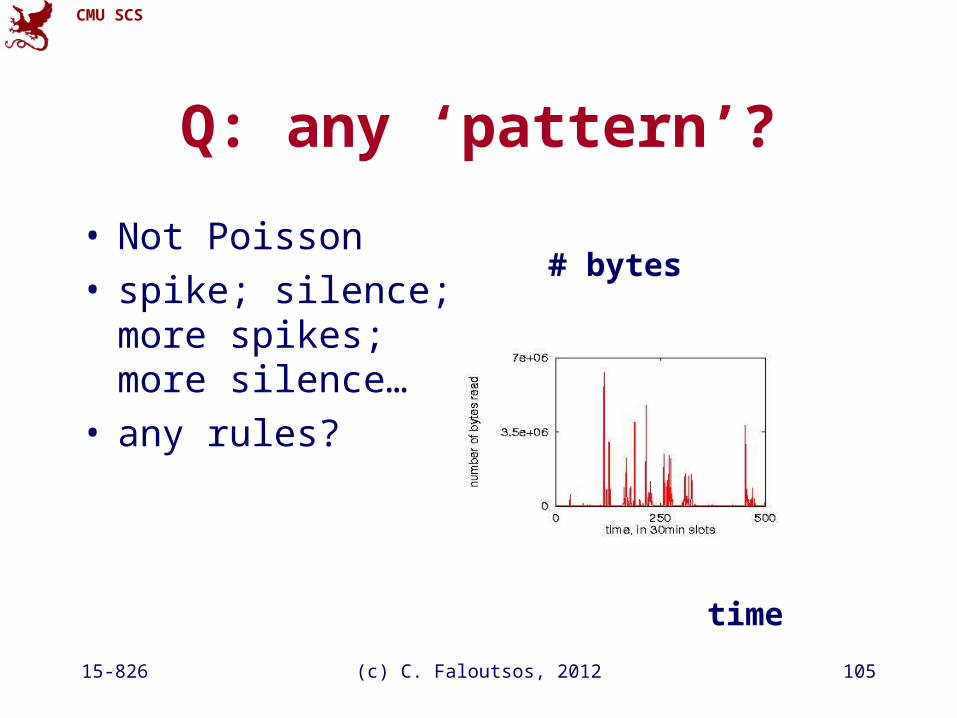
Q: any ‘pattern’?
time
# bytes• Not Poisson• spike; silence; more
spikes; more silence…• any rules?
CMU SCS
15-826 (c) C. Faloutsos, 2012 106
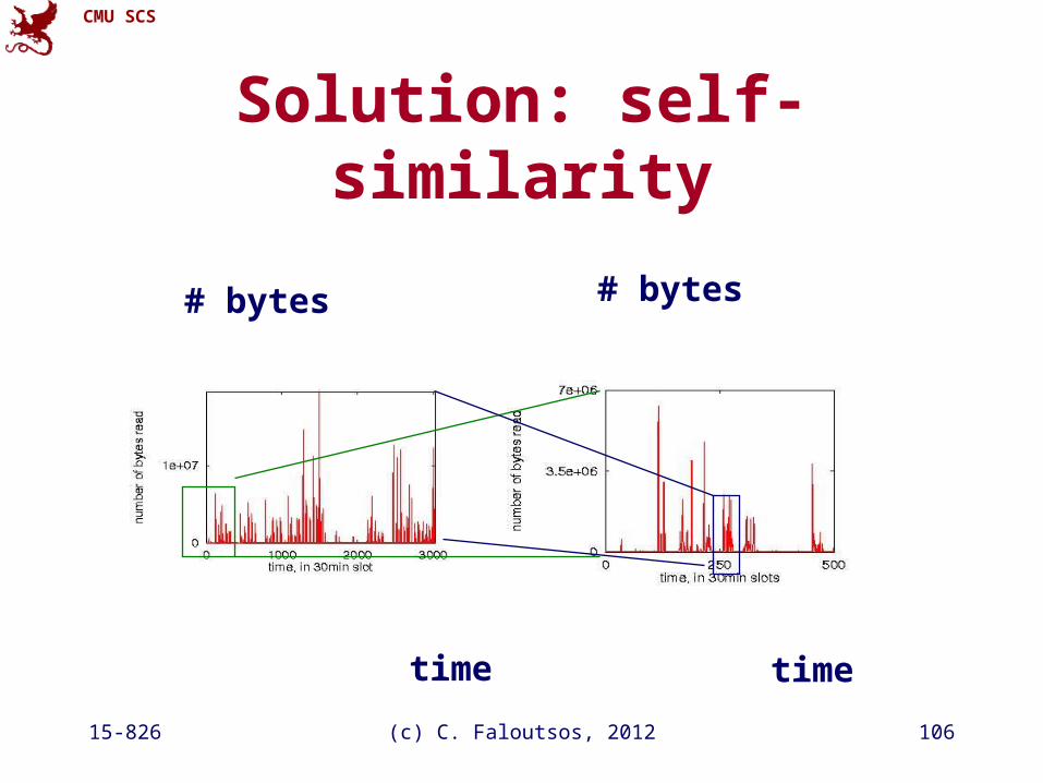
Solution: self-similarity
# bytes
time time
# bytes
CMU SCS
15-826 (c) C. Faloutsos, 2012 107
But:
• Q1: How to generate realistic traces; extrapolate; give guarantees?
• Q2: How to estimate the model parameters?
CMU SCS
15-826 (c) C. Faloutsos, 2012 108
Outline
• Motivation
• ...
• Linear Forecasting
• Bursty traffic - fractals and multifractals– Problem– Main idea (80/20, Hurst exponent)– Results

CMU SCS
15-826 (c) C. Faloutsos, 2012 109
Approach
• Q1: How to generate a sequence, that is– bursty– self-similar– and has similar queue length distributions
CMU SCS
15-826 (c) C. Faloutsos, 2012 110
Approach
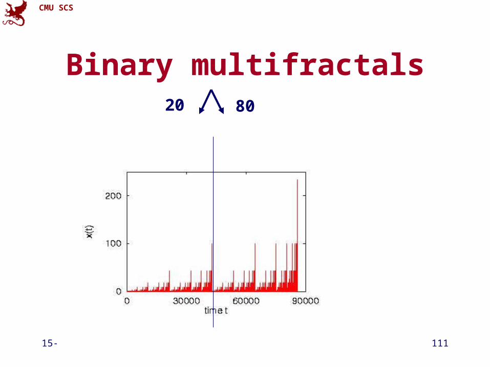
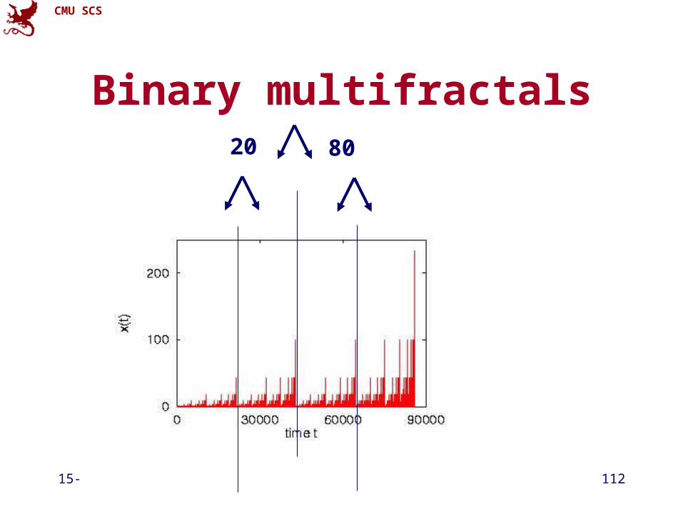
• A: ‘binomial multifractal’ [Wang+02]
• ~ 80-20 ‘law’:– 80% of bytes/queries etc on first half– repeat recursively
• b: bias factor (eg., 80%)
CMU SCS
15-826 (c) C. Faloutsos, 2012 111
Binary multifractals20 80
CMU SCS
15-826 (c) C. Faloutsos, 2012 112
Binary multifractals20 80
CMU SCS
15-826 (c) C. Faloutsos, 2012 113
Parameter estimation
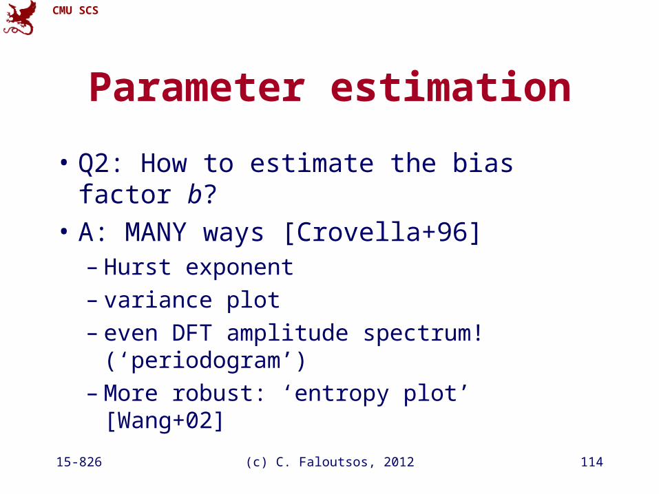
• Q2: How to estimate the bias factor b?
CMU SCS
15-826 (c) C. Faloutsos, 2012 114
Parameter estimation
• Q2: How to estimate the bias factor b?
• A: MANY ways [Crovella+96]– Hurst exponent– variance plot– even DFT amplitude spectrum! (‘periodogram’)– More robust: ‘entropy plot’ [Wang+02]
CMU SCS
15-826 (c) C. Faloutsos, 2012 115
Entropy plot
• Rationale:– burstiness: inverse of uniformity– entropy measures uniformity of a distribution– find entropy at several granularities, to see
whether/how our distribution is close to uniform.
CMU SCS
15-826 (c) C. Faloutsos, 2012 116
Entropy plot
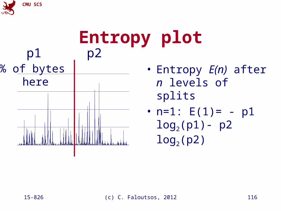
• Entropy E(n) after n levels of splits
• n=1: E(1)= - p1 log2(p1)- p2 log2(p2)
p1 p2% of bytes
here
CMU SCS
15-826 (c) C. Faloutsos, 2012 117
Entropy plot
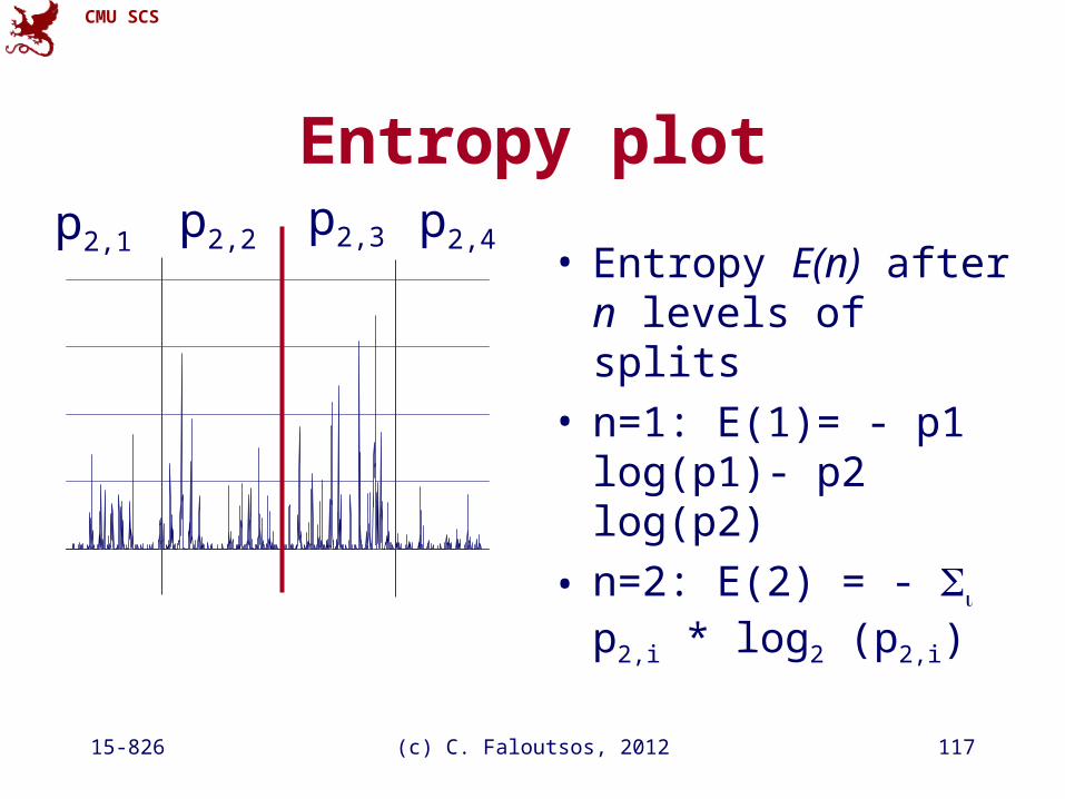
• Entropy E(n) after n levels of splits
• n=1: E(1)= - p1 log(p1)- p2 log(p2)
• n=2: E(2) = - p2,i * log2 (p2,i)
p2,1 p2,2 p2,3 p2,4
CMU SCS
15-826 (c) C. Faloutsos, 2012 118
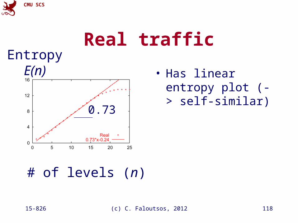
Real traffic
• Has linear entropy plot (-> self-similar)
# of levels (n)
EntropyE(n)
0.73
CMU SCS
15-826 (c) C. Faloutsos, 2012 119
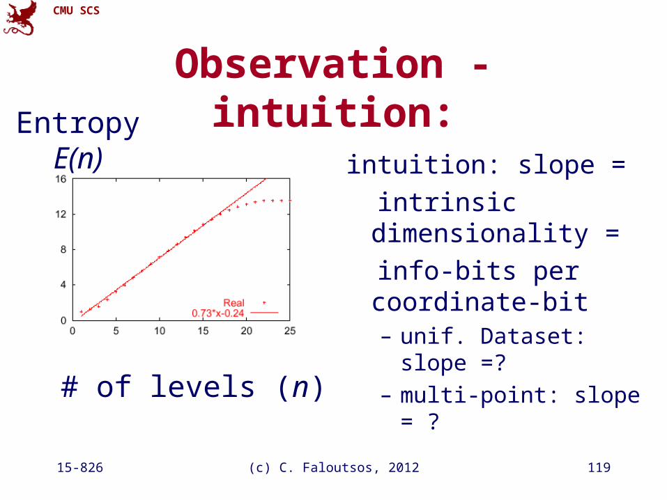
Observation - intuition:
intuition: slope =
intrinsic dimensionality =
info-bits per coordinate-bit– unif. Dataset: slope =?
– multi-point: slope = ?
# of levels (n)
EntropyE(n)
CMU SCS
15-826 (c) C. Faloutsos, 2012 120
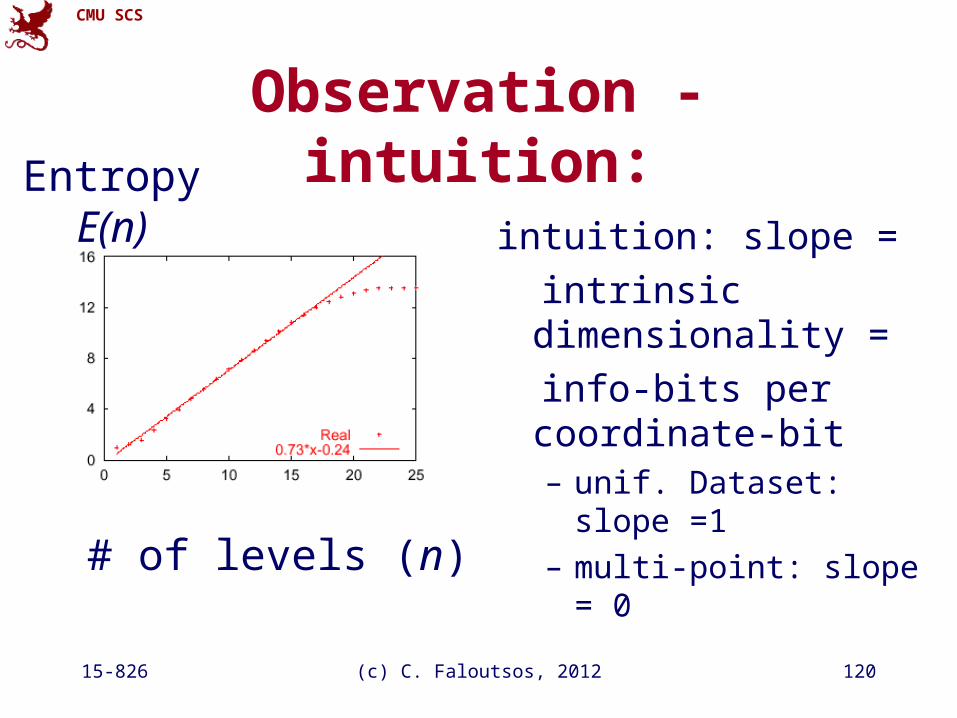
Observation - intuition:
intuition: slope =
intrinsic dimensionality =
info-bits per coordinate-bit– unif. Dataset: slope =1
– multi-point: slope = 0
# of levels (n)
EntropyE(n)
CMU SCS
15-826 (c) C. Faloutsos, 2012 121
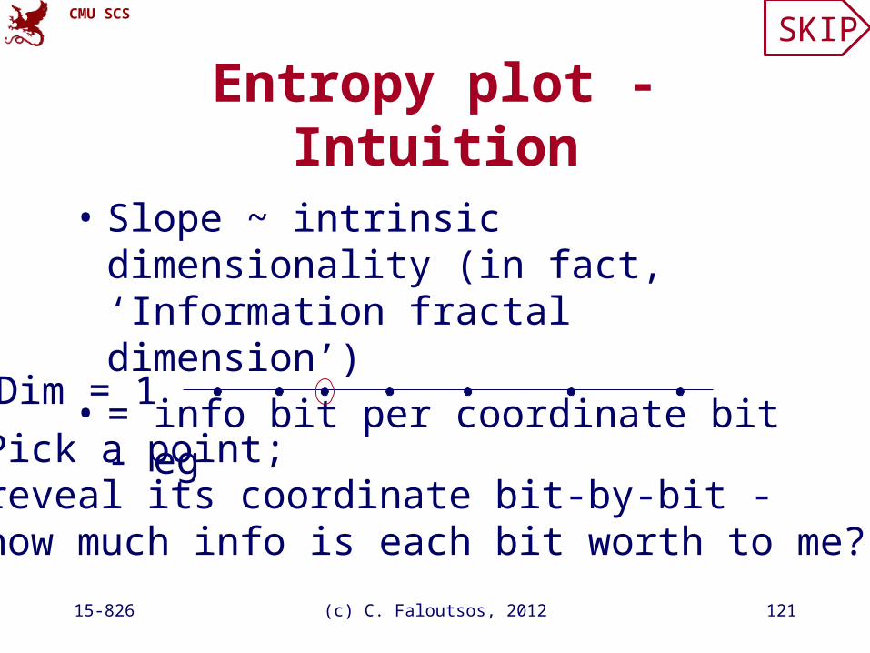
Entropy plot - Intuition
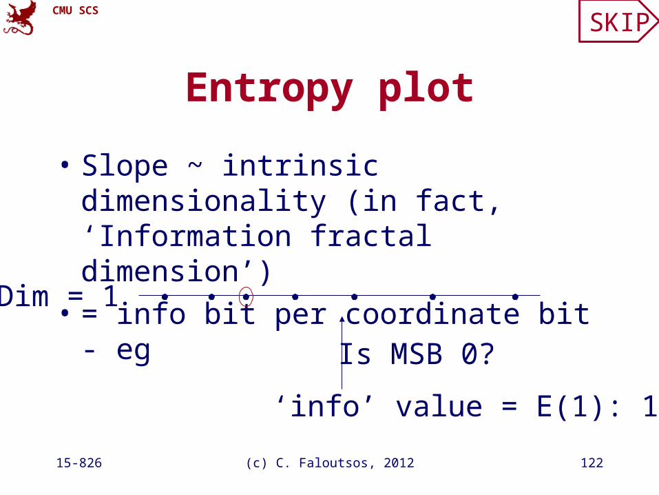
• Slope ~ intrinsic dimensionality (in fact, ‘Information fractal dimension’)
• = info bit per coordinate bit - eg
Dim = 1
Pick a point; reveal its coordinate bit-by-bit -how much info is each bit worth to me?
SKIP
CMU SCS
15-826 (c) C. Faloutsos, 2012 122
Entropy plot
• Slope ~ intrinsic dimensionality (in fact, ‘Information fractal dimension’)
• = info bit per coordinate bit - eg
Dim = 1
Is MSB 0?
‘info’ value = E(1): 1 bit
SKIP
CMU SCS
15-826 (c) C. Faloutsos, 2012 123
Entropy plot
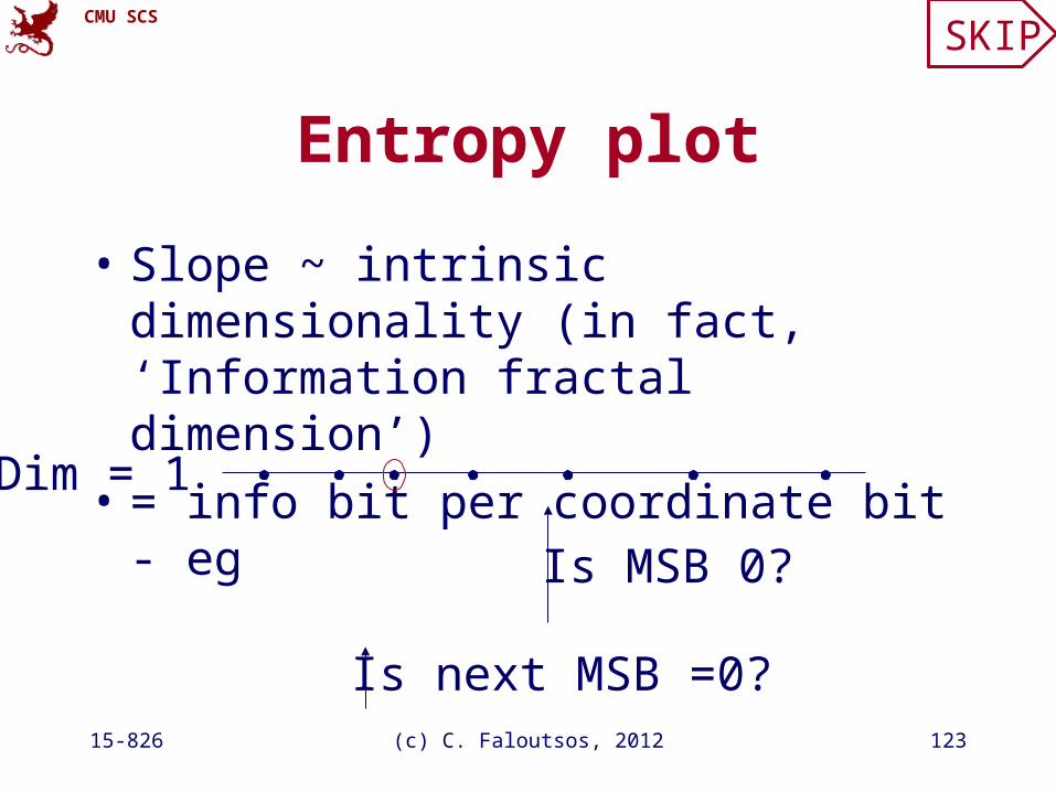
• Slope ~ intrinsic dimensionality (in fact, ‘Information fractal dimension’)
• = info bit per coordinate bit - eg
Dim = 1
Is MSB 0?
Is next MSB =0?
SKIP
CMU SCS
15-826 (c) C. Faloutsos, 2012 124
Entropy plot
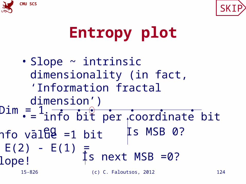
• Slope ~ intrinsic dimensionality (in fact, ‘Information fractal dimension’)
• = info bit per coordinate bit - eg
Dim = 1
Is MSB 0?
Is next MSB =0?
Info value =1 bit= E(2) - E(1) =slope!
SKIP
CMU SCS
15-826 (c) C. Faloutsos, 2012 125
Entropy plot
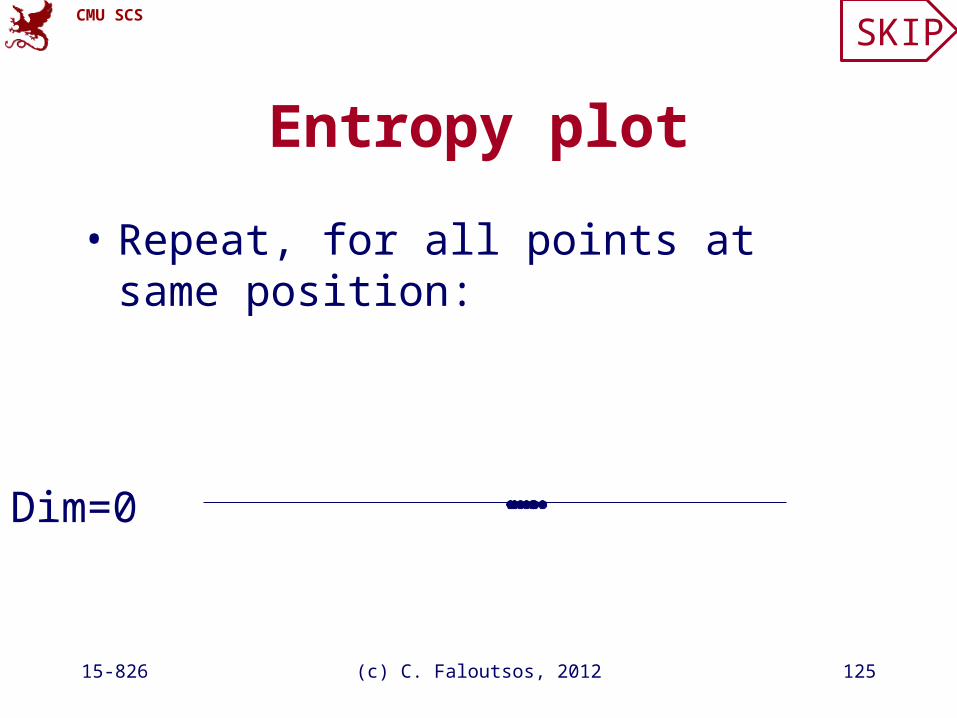
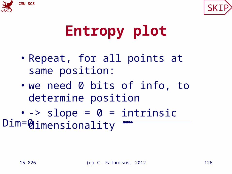
• Repeat, for all points at same position:
Dim=0
SKIP
CMU SCS
15-826 (c) C. Faloutsos, 2012 126
Entropy plot
• Repeat, for all points at same position:
• we need 0 bits of info, to determine position
• -> slope = 0 = intrinsic dimensionality
Dim=0
SKIP
CMU SCS
15-826 (c) C. Faloutsos, 2012 127
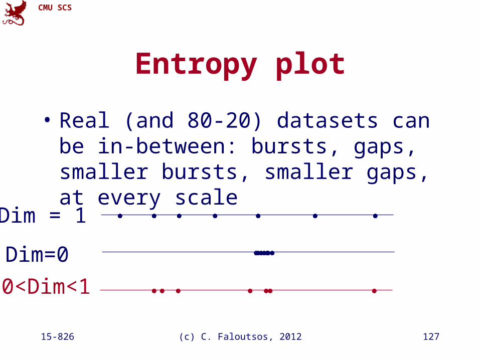
Entropy plot
• Real (and 80-20) datasets can be in-between: bursts, gaps, smaller bursts, smaller gaps, at every scale
Dim = 1
Dim=0
0<Dim<1

CMU SCS
15-826 (c) C. Faloutsos, 2012 128
(Fractals, again)
• What set of points could have behavior between point and line?
CMU SCS
15-826 (c) C. Faloutsos, 2012 129
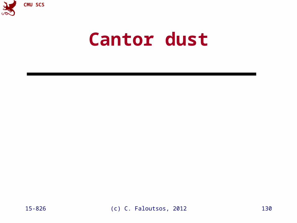
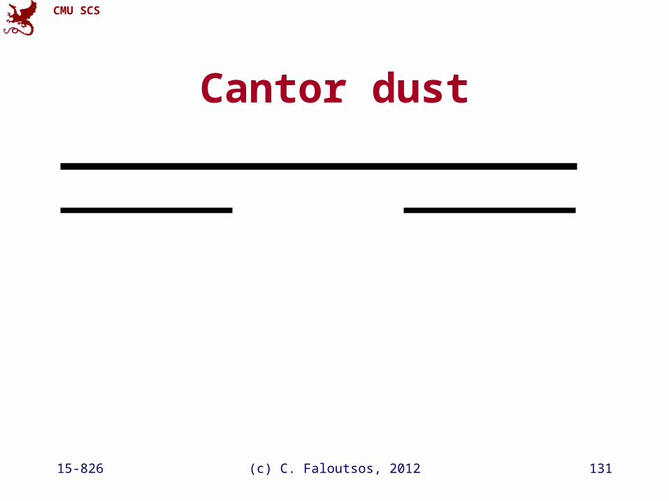
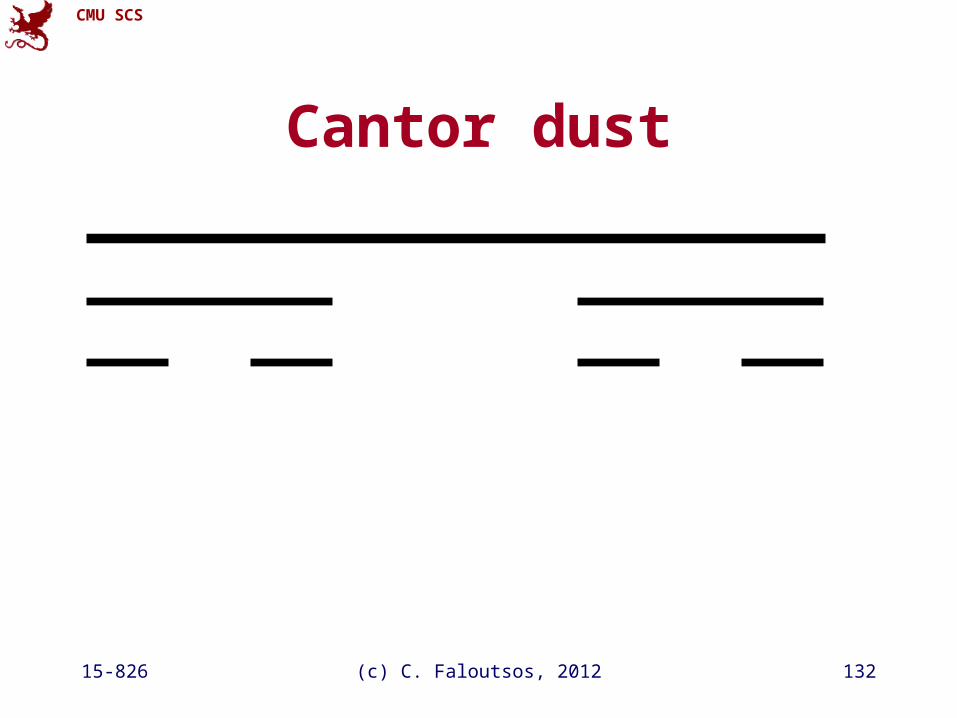
Cantor dust
• Eliminate the middle third
• Recursively!
CMU SCS
15-826 (c) C. Faloutsos, 2012 130
Cantor dust
CMU SCS
15-826 (c) C. Faloutsos, 2012 131
Cantor dust
CMU SCS
15-826 (c) C. Faloutsos, 2012 132
Cantor dust

CMU SCS
15-826 (c) C. Faloutsos, 2012 133
Cantor dust
CMU SCS
15-826 (c) C. Faloutsos, 2012 134
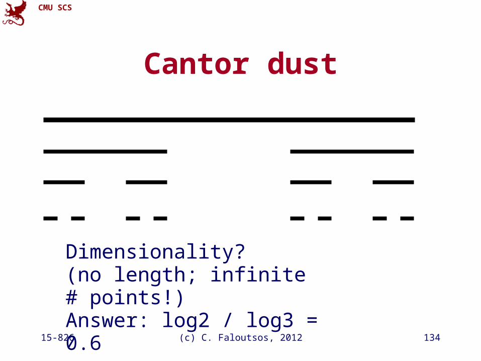
Dimensionality?(no length; infinite # points!)Answer: log2 / log3 = 0.6
Cantor dust
CMU SCS
15-826 (c) C. Faloutsos, 2012 135
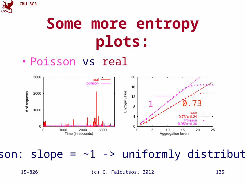
Some more entropy plots:
• Poisson vs real
Poisson: slope = ~1 -> uniformly distributed
1 0.73
CMU SCS
15-826 (c) C. Faloutsos, 2012 136
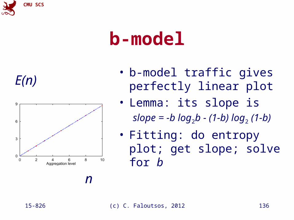
b-model
• b-model traffic gives perfectly linear plot
• Lemma: its slope isslope = -b log2b - (1-b) log2 (1-b)
• Fitting: do entropy plot; get slope; solve for b
E(n)
n
CMU SCS
15-826 (c) C. Faloutsos, 2012 137
Outline
• Motivation
• ...
• Linear Forecasting
• Bursty traffic - fractals and multifractals– Problem– Main idea (80/20, Hurst exponent)– Experiments - Results
CMU SCS
15-826 (c) C. Faloutsos, 2012 138
Experimental setup
• Disk traces (from HP [Wilkes 93])
• web traces from LBLhttp://repository.cs.vt.edu/lbl-conn-7.tar.Z
CMU SCS
15-826 (c) C. Faloutsos, 2012 139
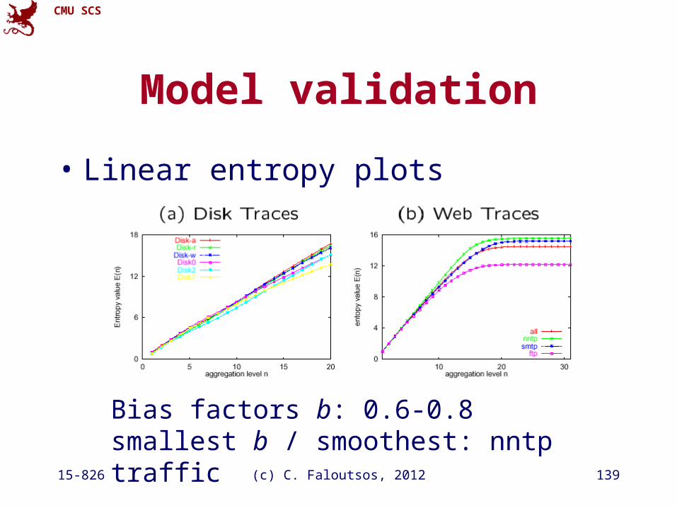
Model validation
• Linear entropy plots
Bias factors b: 0.6-0.8 smallest b / smoothest: nntp traffic
CMU SCS
15-826 (c) C. Faloutsos, 2012 140
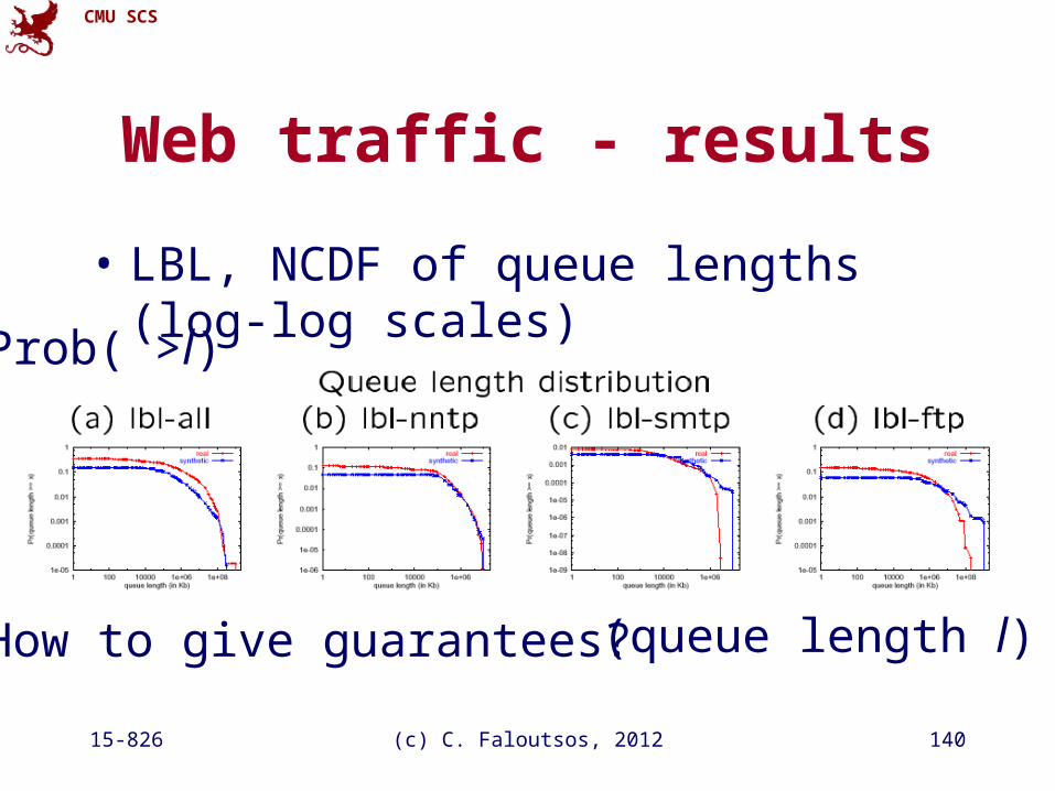
Web traffic - results
• LBL, NCDF of queue lengths (log-log scales)
(queue length l)
Prob( >l)
How to give guarantees?
CMU SCS
15-826 (c) C. Faloutsos, 2012 141
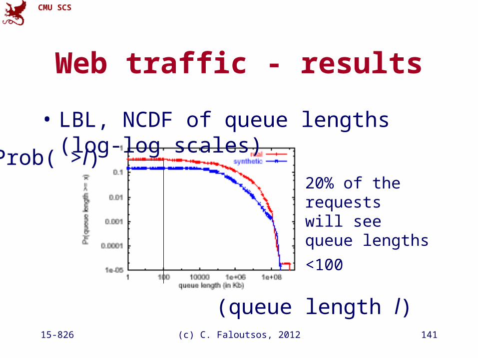
Web traffic - results
• LBL, NCDF of queue lengths (log-log scales)
(queue length l)
Prob( >l)20% of the requestswill see
queue lengths <100
CMU SCS
15-826 (c) C. Faloutsos, 2012 142
Conclusions
• Multifractals (80/20, ‘b-model’, Multiplicative Wavelet Model (MWM)) for analysis and synthesis of bursty traffic
CMU SCS
15-826 (c) C. Faloutsos, 2012 143
Books
• Fractals: Manfred Schroeder: Fractals, Chaos, Power Laws: Minutes from an Infinite Paradise W.H. Freeman and Company, 1991 (Probably the BEST book on fractals!)
CMU SCS
15-826 (c) C. Faloutsos, 2012 144
Further reading:
• Crovella, M. and A. Bestavros (1996). Self-Similarity in World Wide Web Traffic, Evidence and Possible Causes. Sigmetrics.
• [ieeeTN94] W. E. Leland, M.S. Taqqu, W. Willinger, D.V. Wilson, On the Self-Similar Nature of Ethernet Traffic, IEEE Transactions on Networking, 2, 1, pp 1-15, Feb. 1994.
CMU SCS
15-826 (c) C. Faloutsos, 2012 145
Further reading
• [Riedi+99] R. H. Riedi, M. S. Crouse, V. J. Ribeiro, and R. G. Baraniuk, A Multifractal Wavelet Model with Application to Network Traffic, IEEE Special Issue on
Information Theory, 45. (April 1999), 992-1018. • [Wang+02] Mengzhi Wang, Tara Madhyastha, Ngai Hang
Chang, Spiros Papadimitriou and Christos Faloutsos, Data Mining Meets Performance Evaluation: Fast Algorithms for Modeling Bursty Traffic, ICDE 2002, San Jose, CA, 2/26/2002 - 3/1/2002.
Ent
ropy
plo
ts
CMU SCS
15-826 (c) C. Faloutsos, 2012 146
Outline
• Motivation
• ...
• Linear Forecasting
• Bursty traffic - fractals and multifractals
• Non-linear forecasting
• Conclusions
CMU SCS
15-826 (c) C. Faloutsos, 2012 147
Chaos and non-linearforecasting
CMU SCS
15-826 (c) C. Faloutsos, 2012 148
Reference:
[ Deepay Chakrabarti and Christos Faloutsos F4: Large-Scale Automated Forecasting using Fractals CIKM 2002, Washington DC, Nov. 2002.]
CMU SCS
15-826 (c) C. Faloutsos, 2012 149
Detailed Outline
• Non-linear forecasting– Problem– Idea– How-to– Experiments– Conclusions
CMU SCS
15-826 (c) C. Faloutsos, 2012 150
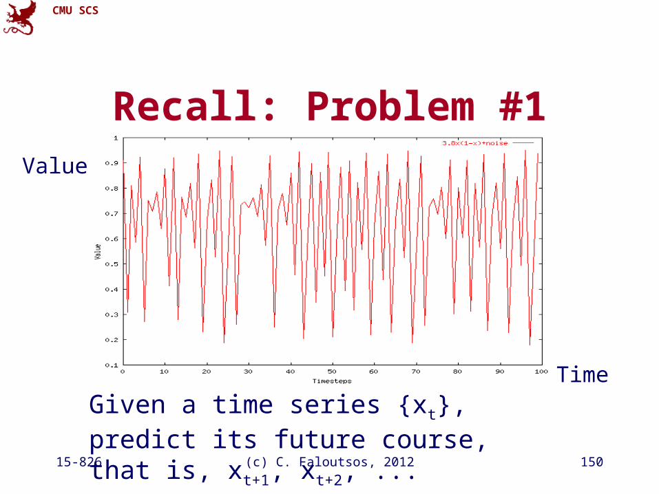
Recall: Problem #1
Given a time series {xt}, predict its future course, that is, xt+1, xt+2, ...
Time
Value
CMU SCS
15-826 (c) C. Faloutsos, 2012 151
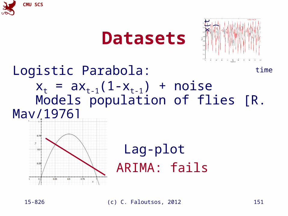
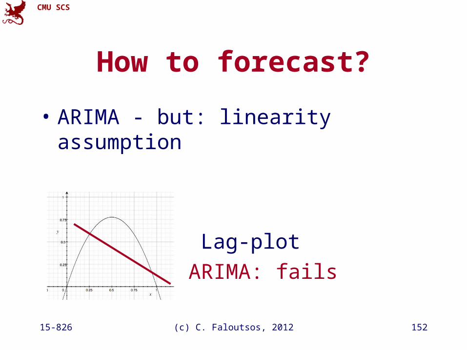
Datasets
Logistic Parabola: xt = axt-1(1-xt-1) + noise Models population of flies [R. May/1976]
time
x(t
)
Lag-plot
ARIMA: fails
CMU SCS
15-826 (c) C. Faloutsos, 2012 152
How to forecast?
• ARIMA - but: linearity assumption
Lag-plot
ARIMA: fails
CMU SCS
15-826 (c) C. Faloutsos, 2012 153
How to forecast?
• ARIMA - but: linearity assumption
• ANSWER: ‘Delayed Coordinate Embedding’ = Lag Plots [Sauer92]
~ nearest-neighbor search, for past incidents
CMU SCS
15-826 (c) C. Faloutsos, 2012 154
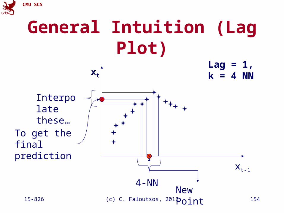
General Intuition (Lag Plot)
xt-1
xxtt
4-NNNew Point
Interpolate these…
To get the final prediction
Lag = 1,k = 4 NN

CMU SCS
15-826 (c) C. Faloutsos, 2012 155
Questions:
• Q1: How to choose lag L?• Q2: How to choose k (the # of NN)?• Q3: How to interpolate?• Q4: why should this work at all?
CMU SCS
15-826 (c) C. Faloutsos, 2012 156
Q1: Choosing lag L
• Manually (16, in award winning system by [Sauer94])
CMU SCS
15-826 (c) C. Faloutsos, 2012 157
Q2: Choosing number of neighbors k
• Manually (typically ~ 1-10)
CMU SCS
15-826 (c) C. Faloutsos, 2012 158
Q3: How to interpolate?
How do we interpolate between the k nearest neighbors?
A3.1: Average
A3.2: Weighted average (weights drop with distance - how?)
CMU SCS
15-826 (c) C. Faloutsos, 2012 159
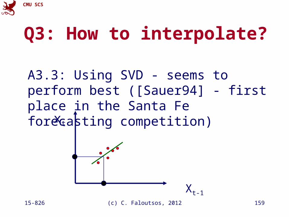
Q3: How to interpolate?
A3.3: Using SVD - seems to perform best ([Sauer94] - first place in the Santa Fe forecasting competition)
Xt-1
xt

CMU SCS
15-826 (c) C. Faloutsos, 2012 160
Q4: Any theory behind it?
A4: YES!
CMU SCS
15-826 (c) C. Faloutsos, 2012 161
Theoretical foundation
• Based on the ‘Takens theorem’ [Takens81]
• which says that long enough delay vectors can do prediction, even if there are unobserved variables in the dynamical system (= diff. equations)
CMU SCS
15-826 (c) C. Faloutsos, 2012 162
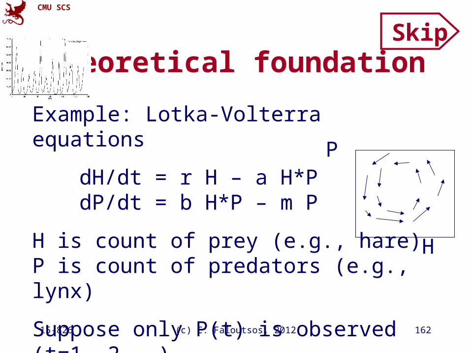
Theoretical foundation
Example: Lotka-Volterra equations
dH/dt = r H – a H*P dP/dt = b H*P – m P
H is count of prey (e.g., hare)P is count of predators (e.g., lynx)
Suppose only P(t) is observed (t=1, 2, …).
H
P
Skip
CMU SCS
15-826 (c) C. Faloutsos, 2012 163
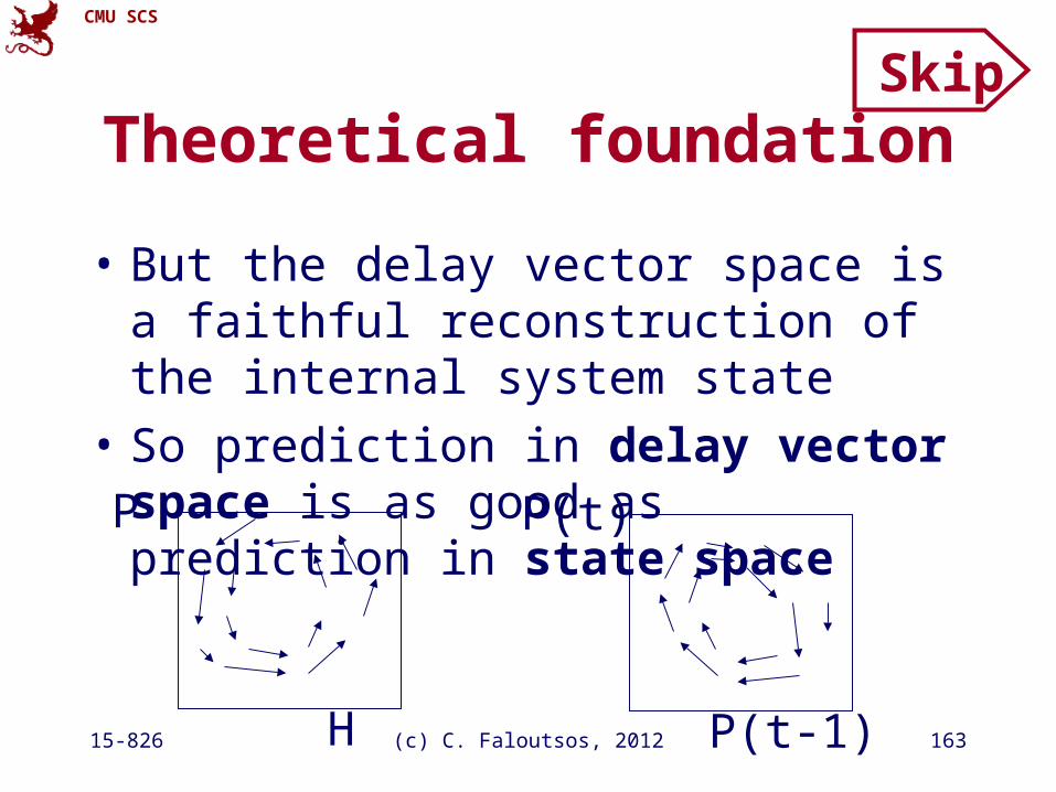
Theoretical foundation
• But the delay vector space is a faithful reconstruction of the internal system state
• So prediction in delay vector space is as good as prediction in state space
Skip
H
P
P(t-1)
P(t)
CMU SCS
15-826 (c) C. Faloutsos, 2012 164
Detailed Outline
• Non-linear forecasting– Problem– Idea– How-to– Experiments– Conclusions
CMU SCS
15-826 (c) C. Faloutsos, 2012 165
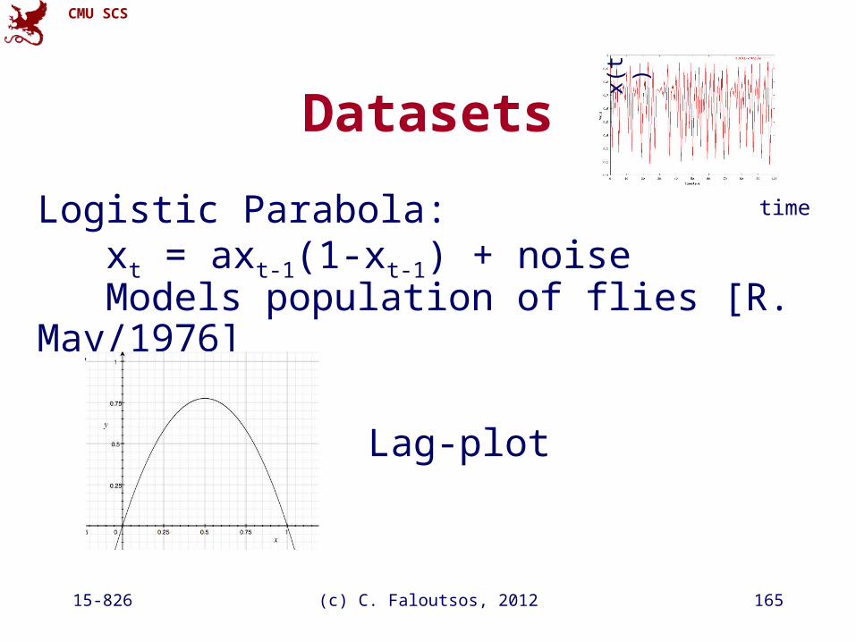
Datasets
Logistic Parabola: xt = axt-1(1-xt-1) + noise Models population of flies [R. May/1976]
time
x(t
)
Lag-plot

CMU SCS
15-826 (c) C. Faloutsos, 2012 166
Datasets
Logistic Parabola: xt = axt-1(1-xt-1) + noise Models population of flies [R. May/1976]
time
x(t
)
Lag-plot
ARIMA: fails
CMU SCS
15-826 (c) C. Faloutsos, 2012 167
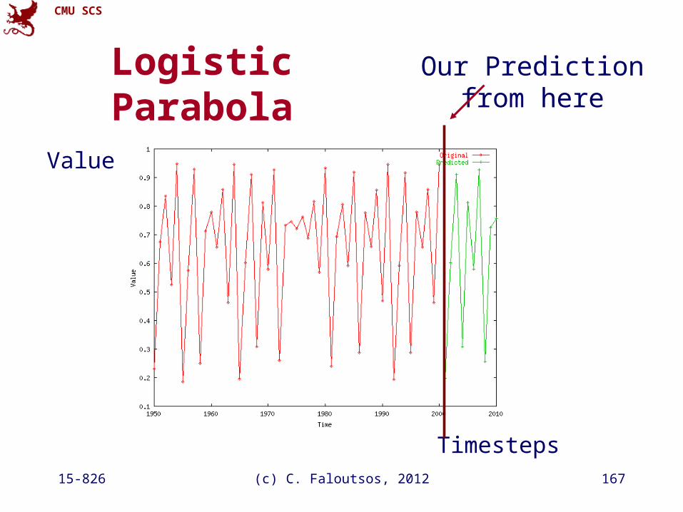
Logistic Parabola
Timesteps
Value
Our Prediction from here
CMU SCS
15-826 (c) C. Faloutsos, 2012 168
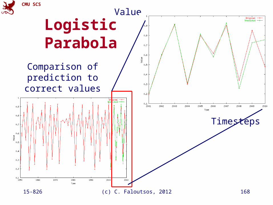
Logistic Parabola
Timesteps
Value
Comparison of prediction to correct values
CMU SCS
15-826 (c) C. Faloutsos, 2012 169
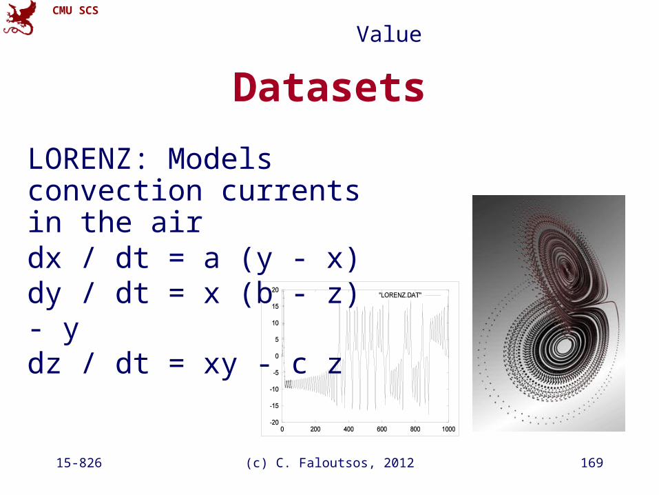
Datasets
LORENZ: Models convection currents in the airdx / dt = a (y - x) dy / dt = x (b - z) - y dz / dt = xy - c z
Value
CMU SCS
15-826 (c) C. Faloutsos, 2012 170
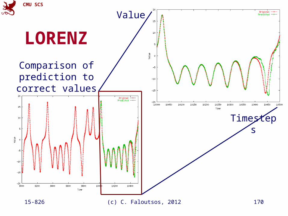
LORENZ
Timesteps
Value
Comparison of prediction to correct values
CMU SCS
15-826 (c) C. Faloutsos, 2012 171
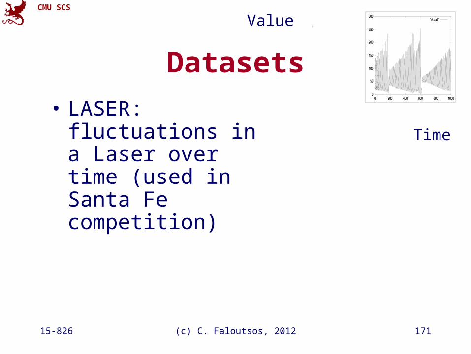
Datasets
Time
Value
• LASER: fluctuations in a Laser over time (used in Santa Fe competition)
CMU SCS
15-826 (c) C. Faloutsos, 2012 172
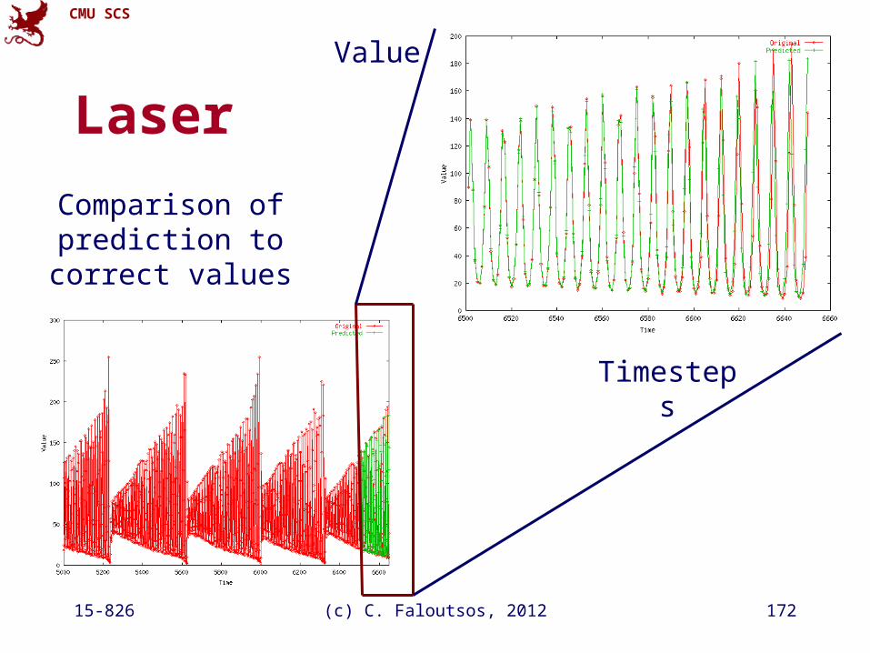
Laser
Timesteps
Value
Comparison of prediction to correct values
CMU SCS
15-826 (c) C. Faloutsos, 2012 173
Conclusions
• Lag plots for non-linear forecasting (Takens’ theorem)
• suitable for ‘chaotic’ signals
CMU SCS
15-826 (c) C. Faloutsos, 2012 174
References
• Deepay Chakrabarti and Christos Faloutsos F4: Large-Scale Automated Forecasting using Fractals CIKM 2002, Washington DC, Nov. 2002.
• Sauer, T. (1994). Time series prediction using delay coordinate embedding. (in book by Weigend and Gershenfeld, below) Addison-Wesley.
• Takens, F. (1981). Detecting strange attractors in fluid turbulence. Dynamical Systems and Turbulence. Berlin: Springer-Verlag.
CMU SCS
15-826 (c) C. Faloutsos, 2012 175
References
• Weigend, A. S. and N. A. Gerschenfeld (1994). Time Series Prediction: Forecasting the Future and Understanding the Past, Addison Wesley. (Excellent collection of papers on chaotic/non-linear forecasting, describing the algorithms behind the winners of the Santa Fe competition.)
CMU SCS
15-826 (c) C. Faloutsos, 2012 176
Overall conclusions
• Similarity search: Euclidean/time-warping; feature extraction and SAMs
CMU SCS
15-826 (c) C. Faloutsos, 2012 177
Overall conclusions
• Similarity search: Euclidean/time-warping; feature extraction and SAMs
• Signal processing: DWT is a powerful tool
CMU SCS
15-826 (c) C. Faloutsos, 2012 178
Overall conclusions
• Similarity search: Euclidean/time-warping; feature extraction and SAMs
• Signal processing: DWT is a powerful tool
• Linear Forecasting: AR (Box-Jenkins) methodology; AWSOM
CMU SCS
15-826 (c) C. Faloutsos, 2012 179
Overall conclusions
• Similarity search: Euclidean/time-warping; feature extraction and SAMs
• Signal processing: DWT is a powerful tool
• Linear Forecasting: AR (Box-Jenkins) methodology; AWSOM
• Bursty traffic: multifractals (80-20 ‘law’)
CMU SCS
15-826 (c) C. Faloutsos, 2012 180
Overall conclusions
• Similarity search: Euclidean/time-warping; feature extraction and SAMs
• Signal processing: DWT is a powerful tool
• Linear Forecasting: AR (Box-Jenkins) methodology; AWSOM
• Bursty traffic: multifractals (80-20 ‘law’)
• Non-linear forecasting: lag-plots (Takens)