15-780: Grad AILecture 7: Optimization

Geoff Gordon

Last time, on Grad AI

Plan graphs

• A way to do propositional planning

• How to build them

• mutex conditions for literals, actions

• How to use them

• conversion to SAT

Optimization & Search

• Classes of optimization problem

• LP, CP, ILP, MILP

• algorithms for solving, and complexity

• constraints, objective, integrality

• How to use DFID, etc. for optimization

• Definition of convexity

Bounds

• Pruning search w/ lower bounds on objective

• Stopping early w/ upper bounds

• Getting bounds from a relaxation of an optimization problem (increase feasible region)

• particularly the LP relaxation of an ILP

Duality

• How to find dual of an LP or ILP

• Interpretations of dual

• linearly combine constraints to get a new constraint orthogonal to objective

• find prices for scarce resources

• game between primal and dual players

• correspondence faces ↔ vertices of feasible regions (doesn’t include objective)

Constrained optimization

Minimization

• Unconstrained: set ∇f(x) = 0

• E.g., minimize

f(x, y) = x2 + y2 + 6x - 4y + 5

∇f(x, y) = (2x + 6, 2y - 4)

(x, y) = (-3, 2)

Equality constraints

• Equality constraint:

minimize f(x) s.t. g(x) = 0

• can’t just set ∇f to 0 (might violate constraint)

• Instead, want gradient along constraint’s normal direction: any motion that decreases objective will violate the constraint

Example

• E.g., minimize x2 + y2 subject to x + y = 2

Lagrange Multipliers

Lagrange multipliers are a way to solve constrained optimization problems.

For example, suppose we want to minimize the function

f !x, y" ! x2 " y2

subject to the constraint

0 ! g!x, y" ! x " y# 2

Here are the constraint surface, the contours of f , and the solution.

lp.nb 3

Lagrange multipliers

• Minimize f(x) s.t. g(x) = 0

• Constraint normal is ∇g

• (1, 1) in our example

• Want ∇f parallel to ∇g

• Equivalently, want ∇f = λ∇g

• λ is a Lagrange multiplier

Lagrange Multipliers

Lagrange multipliers are a way to solve constrained optimization problems.

For example, suppose we want to minimize the function

f !x, y" ! x2 " y2

subject to the constraint

0 ! g!x, y" ! x " y# 2

Here are the constraint surface, the contours of f , and the solution.

lp.nb 3

More than one constraint

• With multiple constraints, use multiple multipliers:

min x2 + y2 + z2 st

x + y = 2

x + z = 2

(2x, 2y, 2z) = λ(1, 1, 0) + µ(1, 0, 1)

Two constraints: the picture

Multiple Constraints: the Picture

The solution to the above equations is

!p ! "4#####3

, q ! "4#####3

, x ! 4#####3

, y! 2#####3

, z ! 2#####3"

Here are the two constraints, together with a level surface of the objective

function. Neither constraint is tangent to the level surface; instead, the

normal to the level surface is a linear combination of the normals to the

two constraint surfaces (with coefficients p and q).

lp.nb 7

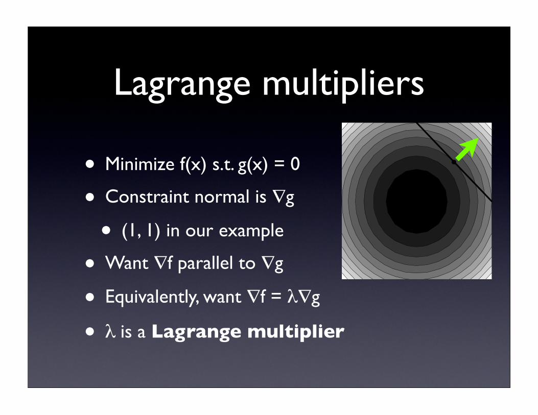
What about inequalities?

• Two cases: if minimum is in interior, can get it by setting ∇f = 0

What about inequalities?

• But if minimum is on boundary, treat as if boundary were an equality constraint (use Lagrange multiplier)

What about inequalities?

• Minimum could be at a corner: two boundary constraints are active

• In n dims, up to n linear inequalities may be active (more in case of degeneracy)

Back to LP

Widgets →

Doo

dads

→w + d ≤ 4

2w + 5d ≤ 12

profit = w + 2d

feasible

Back to LP

max w + 2d st

w + d ≤ 4

2w + 5d ≤ 12

w, d ≥ 0

• In LP we’re minimizing linear fn subject to linear constraints

• So gradients are really easy to compute

Back to LP

• Minimum can’t* occur in interior of feasible region

• In fact we can assume it’s at a vertex

• So to find it, we must check vertices

• How many boundary vertices could there be?

Bases

• With m constraints and n variables, any subset of n constraints might be active

• So up to (m choose n) possibilities

• Given subset, easy to find corresponding vertex (solve linear system)

• Subset = basis

Search

• This is a combinatorial optimization problem, so could use one of our standard search algorithms

• Search space:

• node = basis

• objective = linear function of vertex

• neighbor = ?

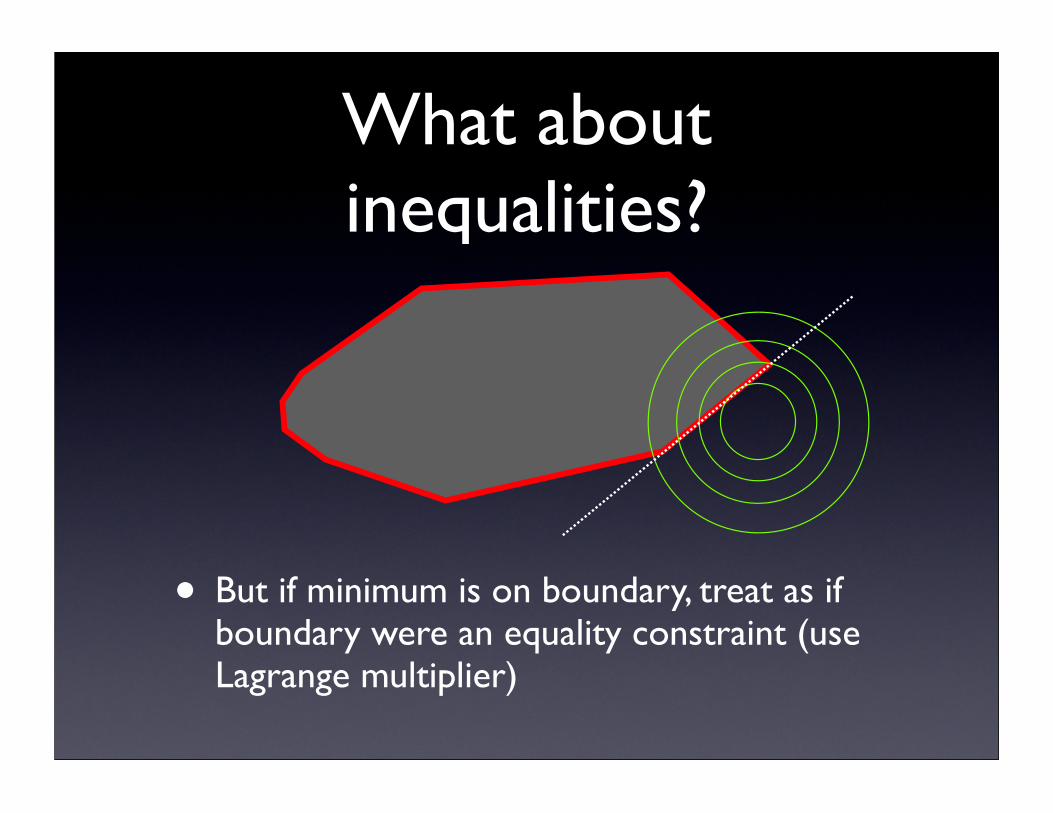
Neighboring bases

• Two bases are neighbors if they share (n-1) of n constraints

• Expanding a node in our search picks one constraint to add and another to delete

Neighbors

Widgets →

Doo

dads

→

Neighbors

Widgets →

Doo

dads

→

Neighbors

Widgets →

Doo

dads

→

Simplex

• Notice that the objective increased monotonically throughout search

• Turns out, this is always possible—leads to a lot of pruning!

• We have just defined the simplex algorithm

• if we pretend that arbitrary vertices are feasible, with an objective that penalizes infeasibility heavily

Duality example

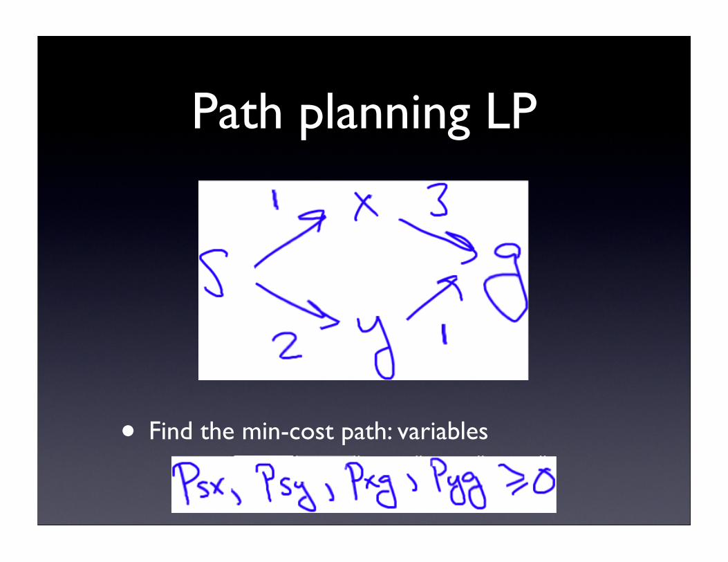
Path planning LP

• Find the min-cost path: variables

Path planning LP

Optimal solution

psy = pyg = 1, psx = pxg = 0, cost 3

Matrix form

Dual

Dual objective

• To get tightest bound, maximize:

Whole thing

Optimal dual solution

0

1

3

3

Any solution which adds a constant to all λs also works

Similarly, could reduce λx as far as 2

Interpretation

• Dual variables are prices on nodes: how much does it cost to start there?

• Dual constraints are local price constraints: edge xg (cost 3) means that node x can’t cost more than 3 + price of node g

Search in ILPs

Simple search algorithm (from last class)

• Run DFS

• node = partial assignment

• neighbor = set one variable

• Prune if a constraint becomes unsatisfiable

• E.g., in 0/1 prob, setting y = 0 in x + 3y ≥ 4

• If we reach a feasible full assignment, calculate its value, keep best

Pruning

• Suggested increasing pruning by adding constraints

• Constraint from best solution so far: objective ≥ M (for maximization problem)

• Constraint from optimal dual solution: objective ≤ M

• Can we find more pruning to do?

First idea

• Analogue of constraint propagation or unit resolution

• When we set a variable x, check constraints containing x to see if they imply a restriction on the domain of some other variable y

• E.g., setting x to 1 in implication constraint (1-x) + y ≥ 1

Example

• 0/1 variables x, y, z

• maximize x subject to

2x + 2y - z ≤ 2

2x - y + z ≤ 2

-x + 2y - z ≤ 0

Example search

Problem w/ constraint propagation

• Constraint propagation doesn’t prune as early as it could:

2x + 2y - z ≤ 2

2x - y + z ≤ 2

-x + 2y - z ≤ 0

• Consider z = 1

Branch and bound

• Each time we fix a variable, solve the resulting LP

• Gives a tighter upper bound on value of objective in this branch

• If this upper bound < value of a previous solution, we can prune

• Called fathoming the branch

Can we do more?

• Yes: we can make bounds tighter by looking at the…

Duality gap

Factory LP

Widgets →

Doo

dads

→w + d ≤ 4

2w + 5d ≤ 12

Duality gap

• We got bound of 5 1/3 either from primal LP relaxation or from dual LP

• Compare to actual best profit of 5 (respecting integrality constraints)

• Difference of 1/3 is duality gap

• Term is also used for ratio 5 / (5 1/3)

• Pretty close to optimal, right?

Unfortunately…

Widgets →

Doo

dads

→ profit = w + 2d

Bad gap

• In this example, duality gap is 3 vs 8.5, or about a ratio of 0.35

• Ratio can be arbitrarily bad

• Aside: can often bound it for classes of ILPs

• e.g., straightforward ILP from MAX SAT has gap no worse than 1-1/e = 0.632…

Early stopping

• A duality gap this large won’t let us prune or stop our search early

• To fix this problem: cutting planes

Cutting plane

• A cutting plane is a new linear constraint that

• cuts off some of the non-integral points in the LP relaxation

• while leaving all integral points feasible

Cutting plane

Widgets →

Doo

dads

→

constraint from dual optimum

cutting plane

How did we find it?

• Recall our optimal dual multipliers (1/3, 1/3):

1/3 (w + d - 4) + 1/3 (2w + 5d - 12) ≤ 0

w + 2d ≤ 16/3 = 5 1/3

• Since w, d are integers, so is w + 2d

• So if w + 2d ≤ 5 1/3, we also have

w + 2d ≤ 5

Gomory cuts

• This cutting plane is the Gomory cut

• First general recipe to find a cut in poly time that’s guaranteed to cut off at least a minimal amount of the LP relaxation’s feasible region

• Might have fractions on both LHS and RHS:

• 2 1/2 w + 3 d ≤ 5 1/3

Gomory cuts

• Find cut for: 2 1/2 w + 3 d ≤ 5 1/3

• Rounding down fractions on LHS can only weaken inequality:

• 2w + 3d ≤ 5 1/3

• And as before, LHS is now integral so RHS fraction is irrelevant:

• 2w + 3d ≤ 5

Other cuts

• In our example, the Gomory cut was perfect: the vertices of the LP are now the solutions of the ILP

• How good is the Gomory cut in general?

• Sadly, not so great.

• Other cuts (not discussed here): intersection cut, problem specific cuts

Cutting planes recipe

• Solve LP relaxation

• Use optimal primal and dual variables to generate a cut

• Add cut to LP (giving a less-relaxed LP) and re-solve

• Repeat until LP’s primal solution is integral

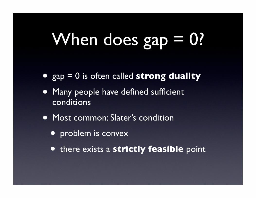
When does gap = 0?

• gap = 0 is often called strong duality

• Many people have defined sufficient conditions

• Most common: Slater’s condition

• problem is convex

• there exists a strictly feasible point

Strictly feasible

• minimize f(x) st

gi(x) ≤ 0, i = 1, 2, …, m

Ax = b

• Strictly feasible point has gi(x) < 0 for all i

• Generalization: strict feasibility need not hold if gi(x) is linear

• so all feasible LPs have gap = 0

Branch and Cut

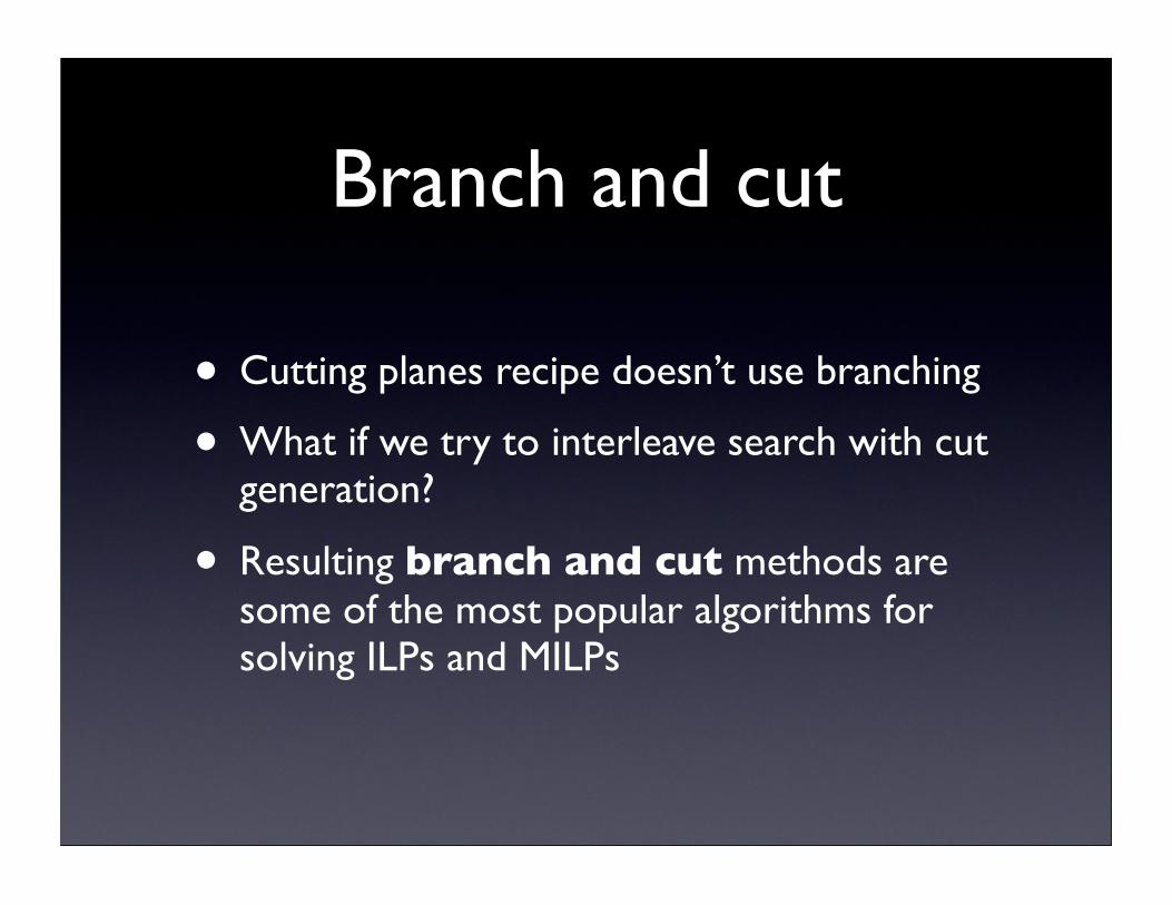
Branch and cut

• Cutting planes recipe doesn’t use branching

• What if we try to interleave search with cut generation?

• Resulting branch and cut methods are some of the most popular algorithms for solving ILPs and MILPs

Recipe

• DFS as for branch and bound

• At each node, solve the LP relaxation

• detect “fathomed” branches

• while not bored

• use dual vars to generate cut, re-solve

• Branch on next variable

• after a branch it may become easier to generate more cuts

Cut generation

• Cuts at a node N are valid at N’s children

• so it’s worth spending more effort higher in the search tree

• General techniques for cut generation are often expensive and/or generate weak cuts

• so people often use problem-specific cuts

Cut lifting

• Sometimes a cut for one branch can be lifted to apply to other branches

• Or we can learn a cut in lifted form to start with

• These cuts are like constraint learning

• Try to compile some of the results of our search to save branching later

Lifted example

• Two constraints from a SAT instance:

• x + y + (1-z) ≥ 1, y + z + w ≥ 1

• Adding them yields

• x + 2y + w ≥ 1

• Trimming yields a cut:

• x + y + w ≥ 1

More generally

• If a variable appears with opposite sign in two constraints, sum them

• x + 2y + z ≥ 1, 2x + y ≥ 1

• 3x + 3y + z ≥ 2

• Then trim the result:

• 2x + 2y + z ≥ 2

Example: robot task assignment

• Team of robots must explore unknown area

Points of interest

Base

Exploration plan

ILP

• Variables (all 0/1):

• zij = task j assigned to robot i

• xijk = robot i uses edge jk

• Cost = path cost - task bonus

• ∑ xijk cijk - ∑ zij tij

Constraints

• For all i, j: ∑k xijk ≥ zij

• For each i, xijk forms a tour from base:

• subtour elimination constraints

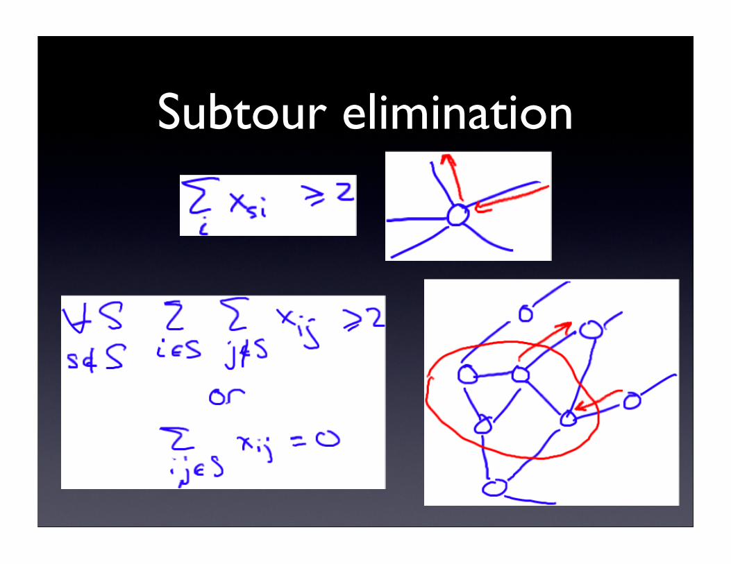
Subtour elimination

Game search

Games

• We will consider games like checkers and chess:

• sequential

• zero-sum

• deterministic, alternating moves

• complete information

• Generalizations later

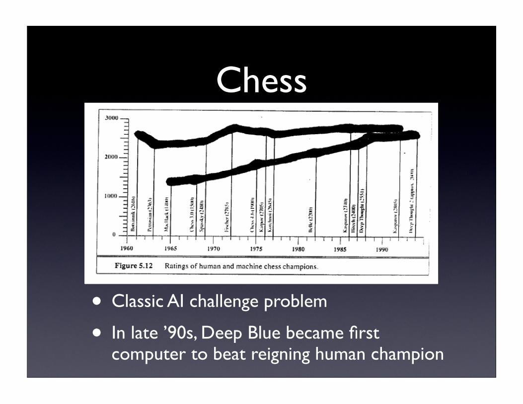
Chess

• Classic AI challenge problem

• In late ’90s, Deep Blue became first computer to beat reigning human champion

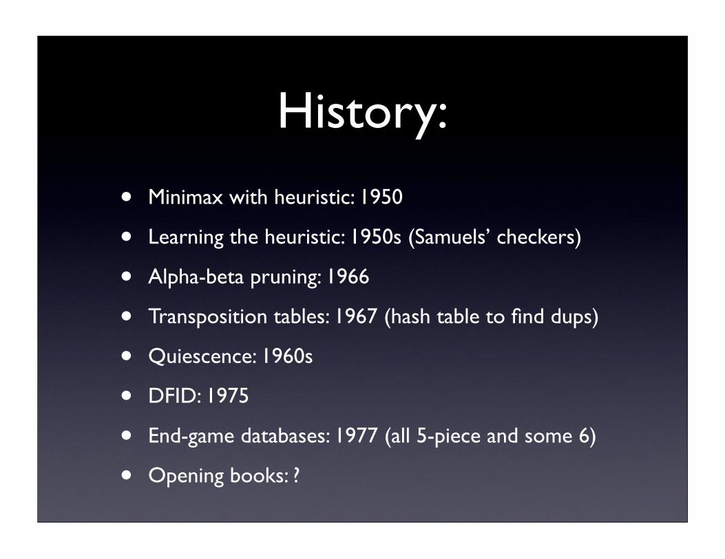
History:

• Minimax with heuristic: 1950

• Learning the heuristic: 1950s (Samuels’ checkers)

• Alpha-beta pruning: 1966

• Transposition tables: 1967 (hash table to find dups)

• Quiescence: 1960s

• DFID: 1975

• End-game databases: 1977 (all 5-piece and some 6)

• Opening books: ?

Game tree

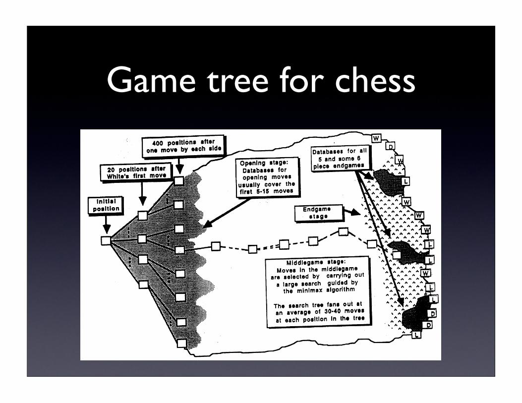
Game tree for chess

Minimax search

• For small games, we can determine the value of each node in the game tree by working backwards from the leaves

• My move: node’s value is maximum over children

• Opponent move: value is minimum over children

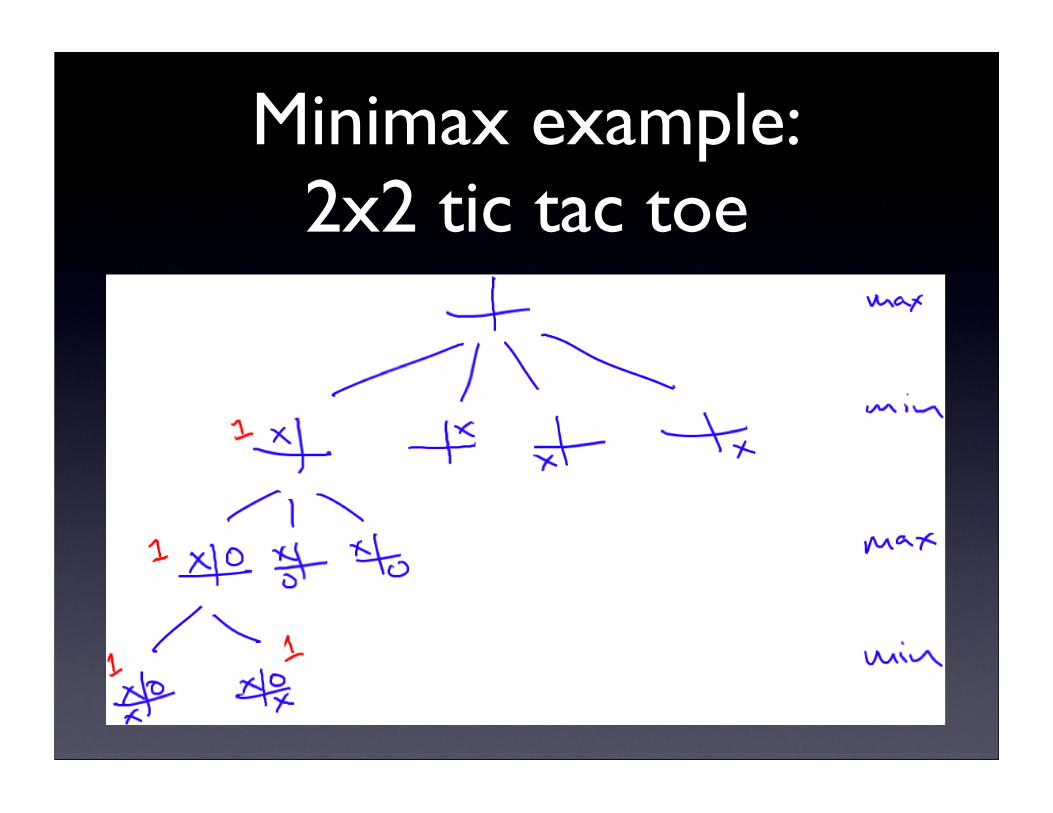
Minimax example:2x2 tic tac toe

Synthetic example

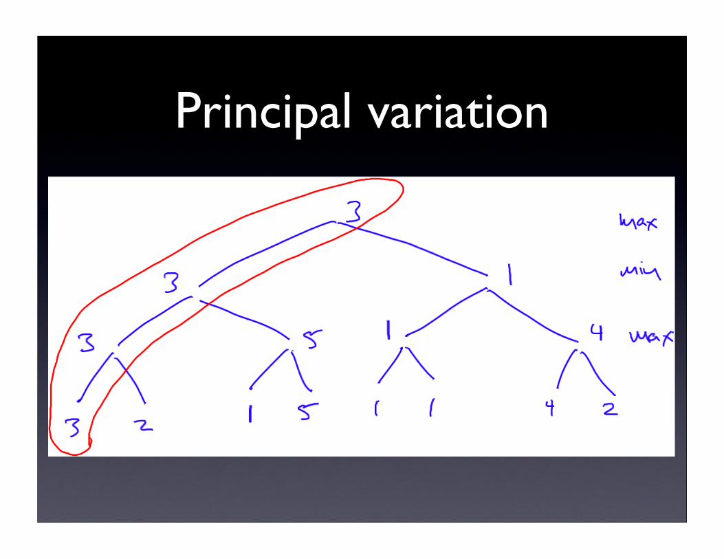
Principal variation