15-780: Grad AILecture 6: Optimization

Geoff Gordon (this lecture)Ziv Bar-Joseph

TAs Geoff Hollinger, Henry Lin

Admin

2

Wait list

There are still several students signed up on the wait list for 15-780If you are one of them, just let us know, and we will move you to the regular course roster

3

Review

4

FOL

Quantifiers, models of FOL expressionsReasoning in FOL

Clause form, SkolemizationUnification and resolutionPropositionalization

Herbrand, Robinson

5

Planning

Representations of timePlanning languages like STRIPS

operators, preconditions, effects

6

Using FOL

7

Knowledge engineering

Identify relevant objects, functions, and predicatesEncode general background knowledge about domain (reusable)Encode specific problem instancePose queries

8

Knowledge engineering

Sadly, next step is also necessary:Debug knowledge base

Severe bug: logical contradictionsLess severe: undesired conclusionsLeast severe: missing conclusions

In general, trace back chain of reasoning until reason for failure is revealed

9

Plan search

10

Plan search

Given a planning problem (start state, operator descriptions, goal)Run standard search algorithms to find planDecisions: search state representation, neighborhood, search algorithm

11

Linear planner

Simplest choice: linear planner Search state = sequence of operatorsNeighbor: add an operator to end of sequenceBind variables as necessary

both operator and binding are choice points

12

Linear planner

Can search forward from start or backward from goalOr mix the twoGoal is often incompletely specifiedExample heuristic: number of open literals

13

Goal: full(M)

14

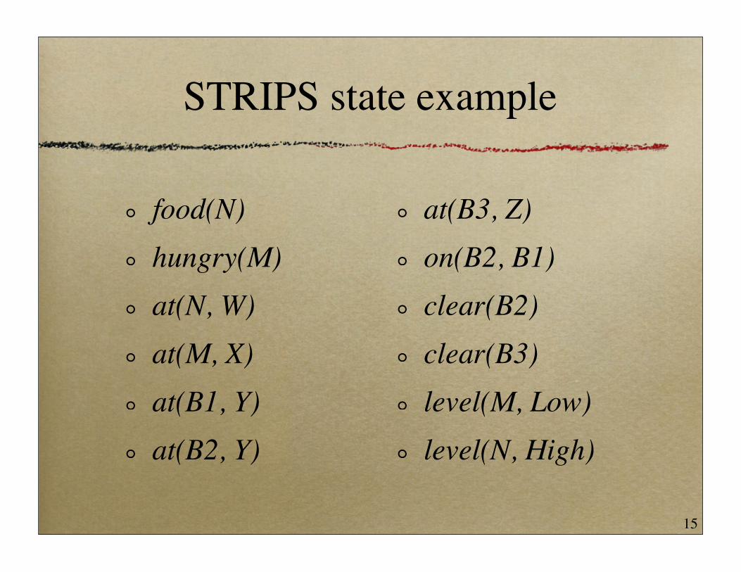
STRIPS state example

food(N)hungry(M)at(N, W)at(M, X)at(B1, Y)at(B2, Y)

at(B3, Z)on(B2, B1)clear(B2)clear(B3)level(M, Low)level(N, High)

15

Linear planner example

Start w/ empty plan [], initial world statePick an operator, e.g.,

Move(from, to)at(M, from), level(M, Low)at(M, to), ¬at(M, from)

16

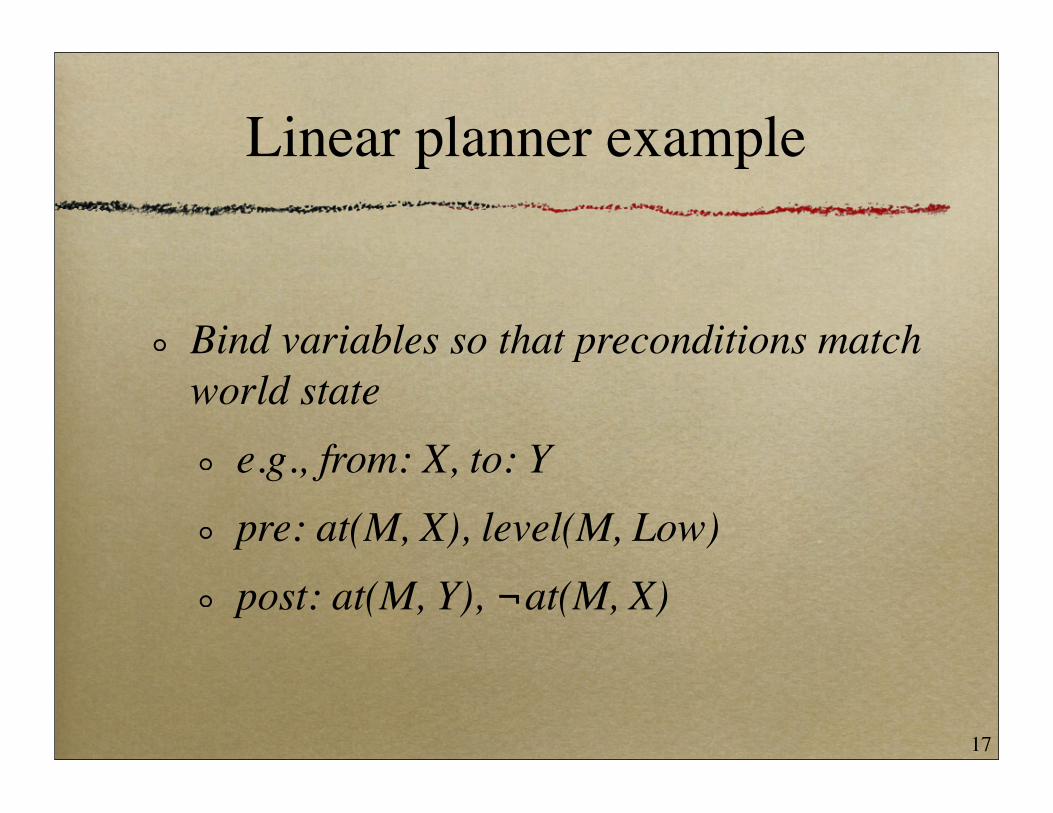
Linear planner example

Bind variables so that preconditions match world state

e.g., from: X, to: Ypre: at(M, X), level(M, Low)post: at(M, Y), ¬at(M, X)

17

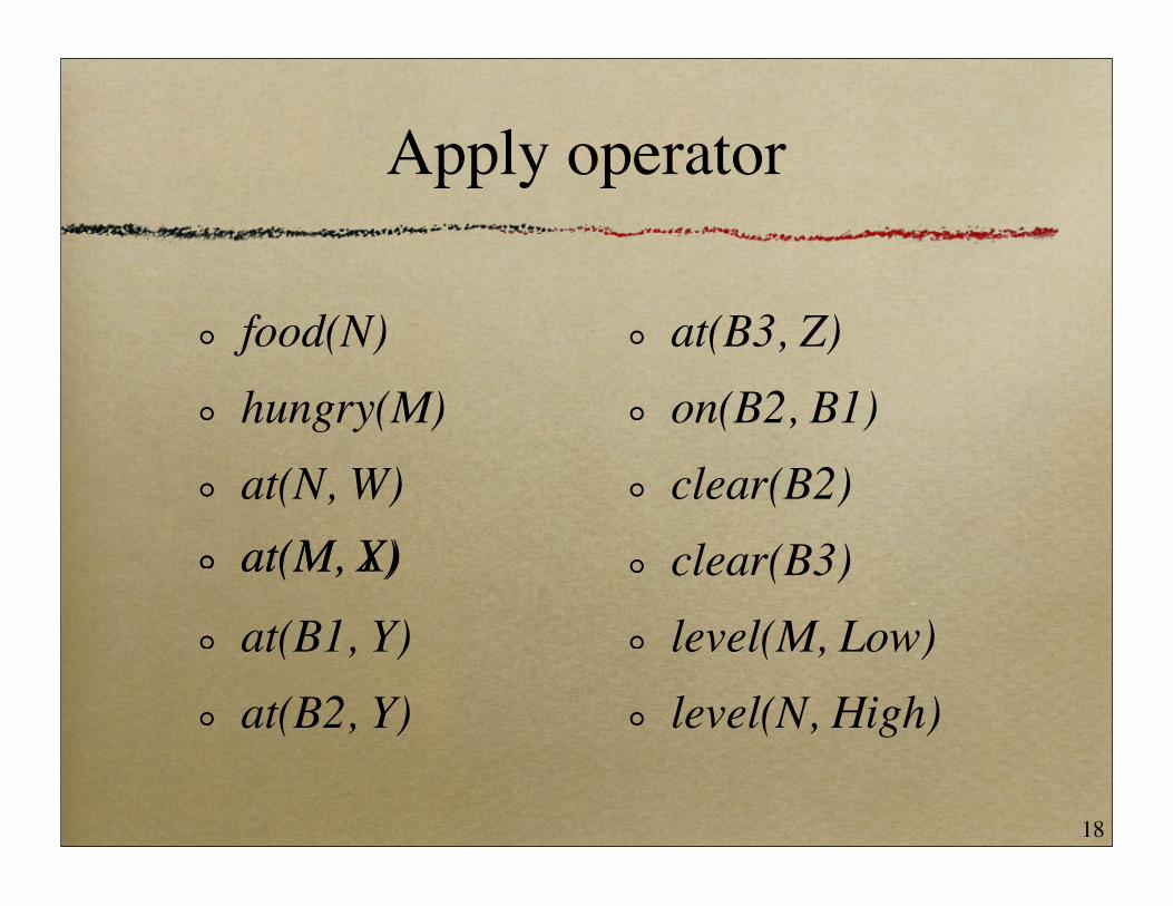
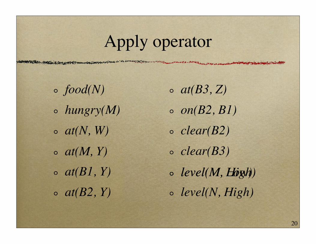
Apply operator

food(N)hungry(M)at(N, W)

at(B1, Y)at(B2, Y)

at(B3, Z)on(B2, B1)clear(B2)clear(B3)level(M, Low)level(N, High)

at(M, X)at(M, Y)

18

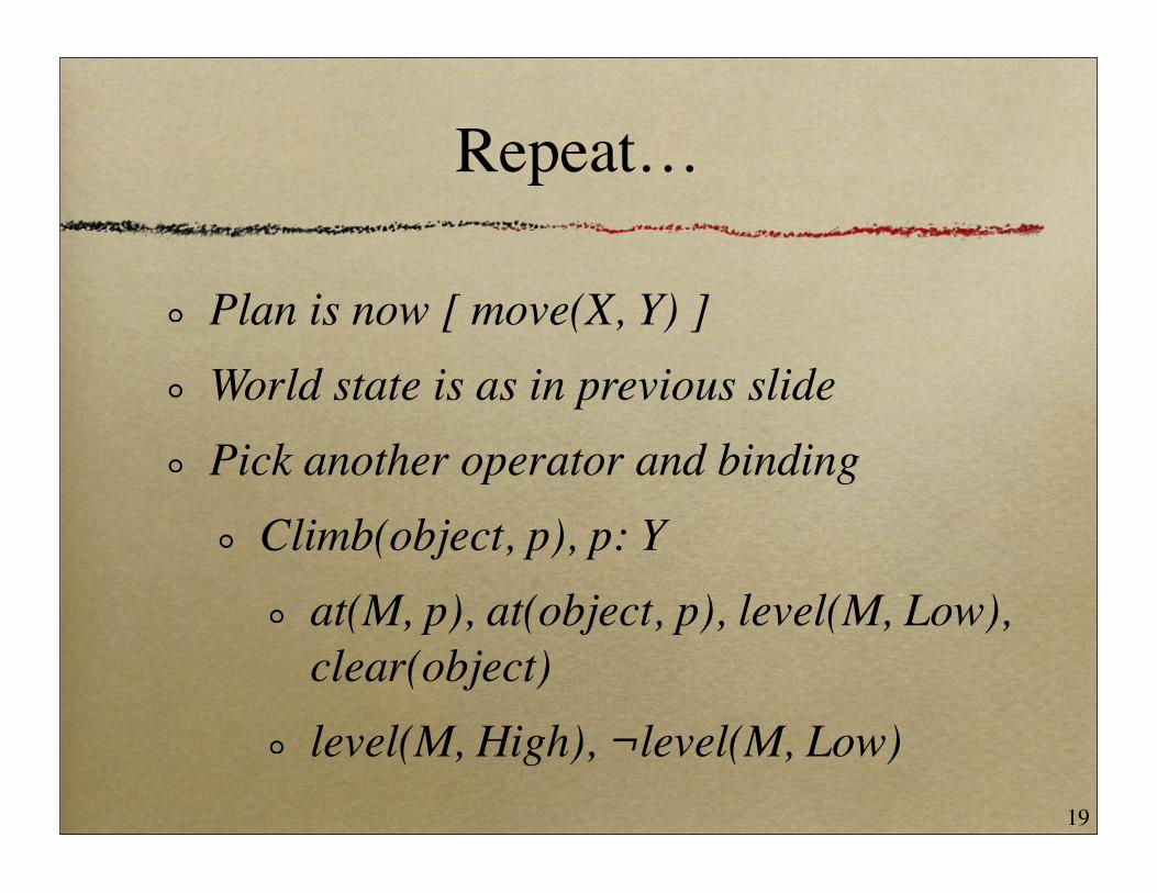
Repeat…

Plan is now [ move(X, Y) ]World state is as in previous slidePick another operator and binding

Climb(object, p), p: Yat(M, p), at(object, p), level(M, Low), clear(object)level(M, High), ¬level(M, Low)

19

Apply operator

food(N)hungry(M)at(N, W)

at(B1, Y)at(B2, Y)

at(B3, Z)on(B2, B1)clear(B2)clear(B3)

level(N, High)

at(M, Y)level(M, Low)level(M, High)

20

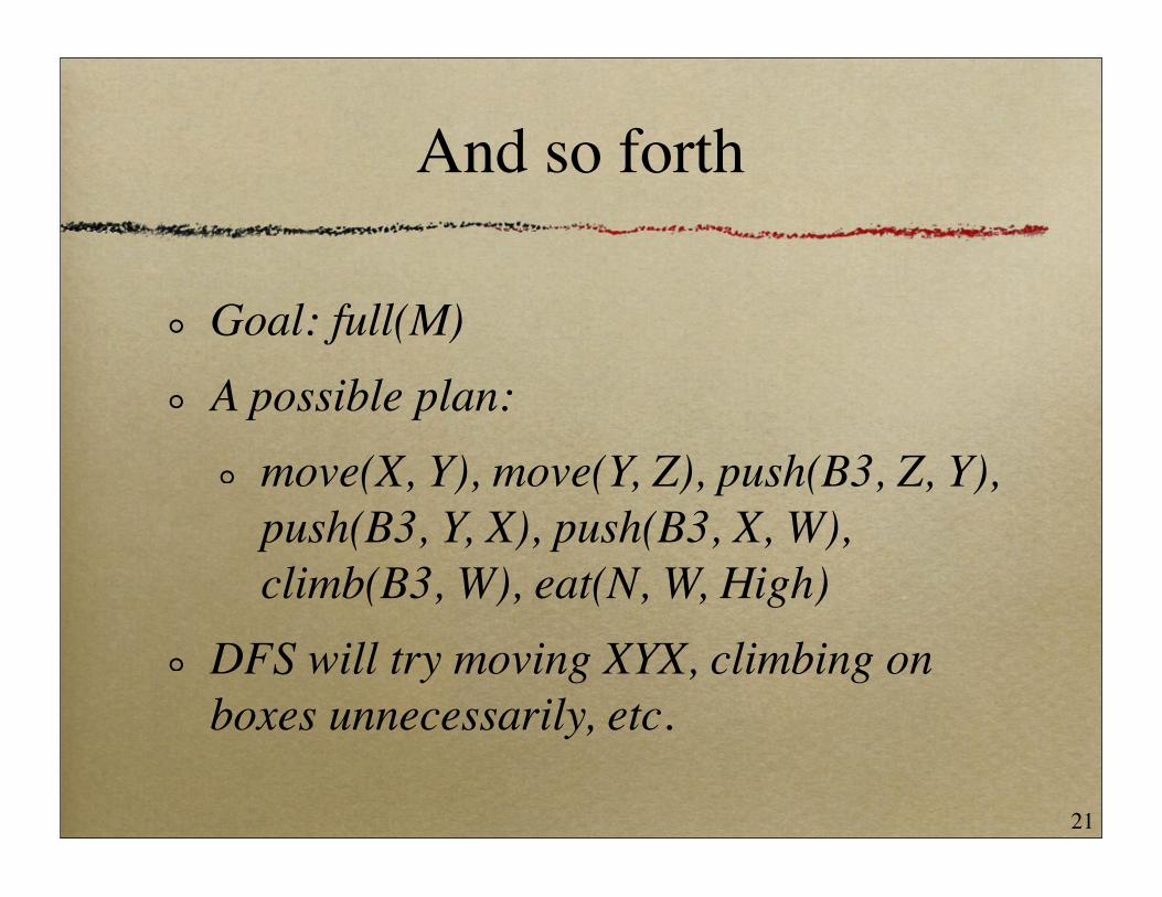
And so forth

Goal: full(M)A possible plan:

move(X, Y), move(Y, Z), push(B3, Z, Y), push(B3, Y, X), push(B3, X, W), climb(B3, W), eat(N, W, High)

DFS will try moving XYX, climbing on boxes unnecessarily, etc.

21

Partial-order planner

Linear planner can be wasteful: backtrack undoes most recent action, rather than one that might have caused failurePartial order planner tries to fix thisAvoids committing to details of plan until it has to (principle of least commitment)

22

Partial-order planner

Search state:set of operators (partially bound)ordering constraintscausal links (also called guards)open preconditions

23

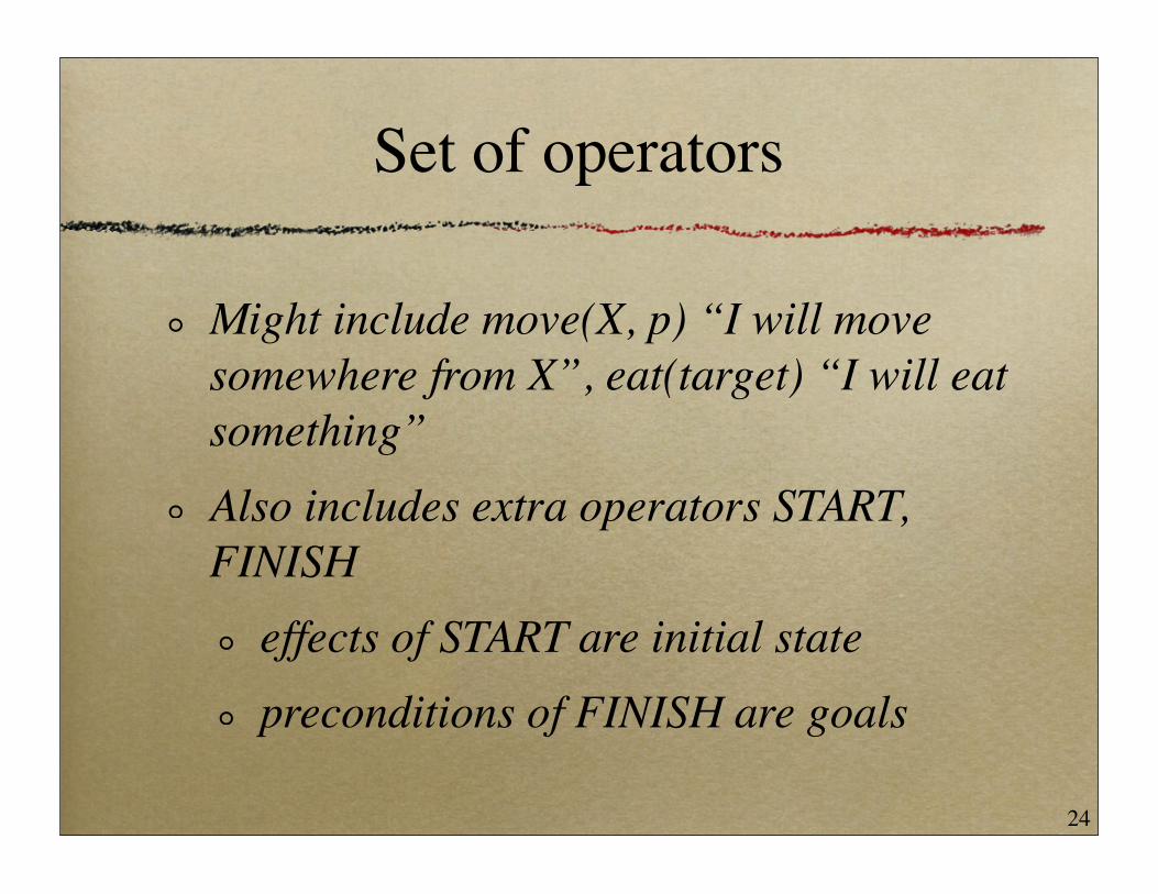
Set of operators

Might include move(X, p) “I will move somewhere from X”, eat(target) “I will eat something”Also includes extra operators START, FINISH

effects of START are initial statepreconditions of FINISH are goals

24

Partial ordering

START move(X, p)

eat(N)

FINISH

push(B3, r, q)

25

Guards

Describe where preconditions are satisfied

START move(X, p)

eat(N)

FINISH

push(B3, r, q)

at(M, X)full(M)

26

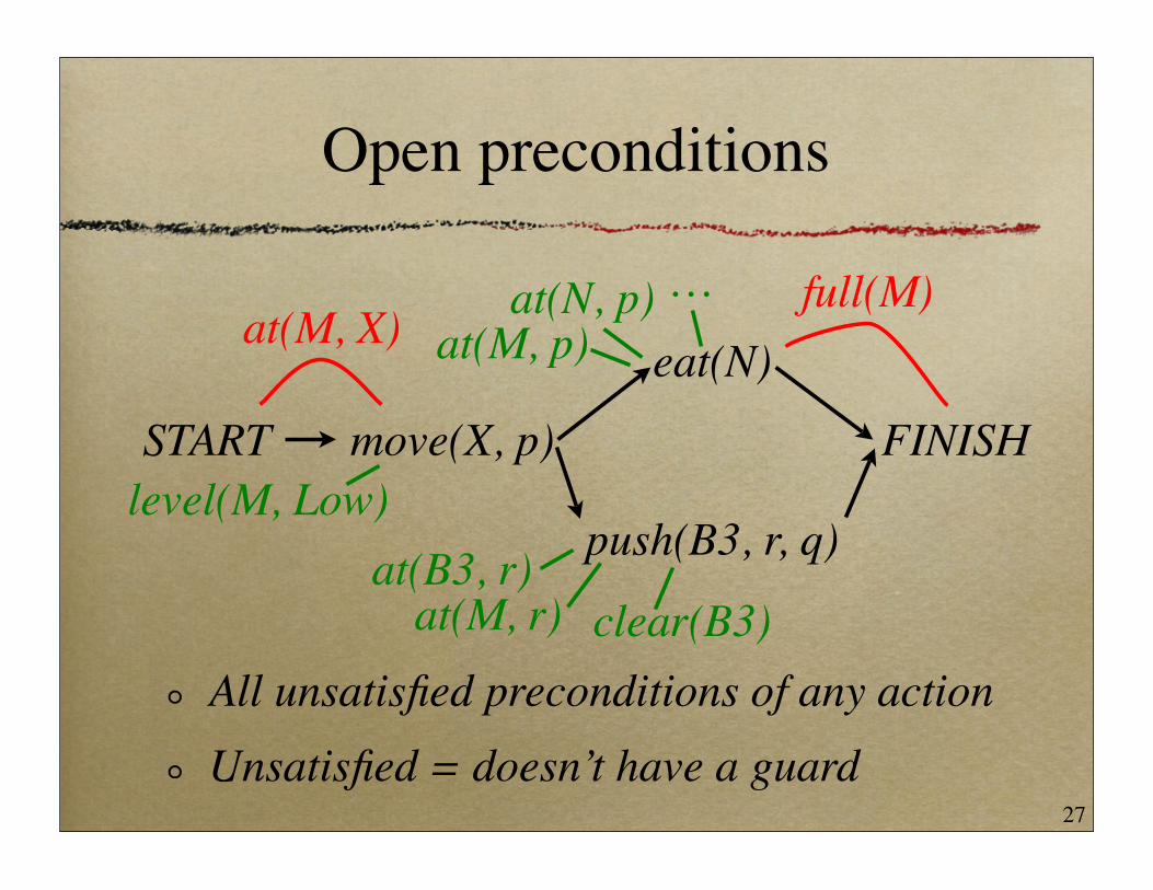
Open preconditions

All unsatisfied preconditions of any actionUnsatisfied = doesn’t have a guard

START move(X, p)

eat(N)

FINISH

push(B3, r, q)

at(M, X)full(M)at(N, p)

at(M, p)

at(B3, r)level(M, Low)

at(M, r) clear(B3)

…

27

Partial-order planner

Neighborhood: plan refinementAdd an operator, guard, or ordering constraint

28

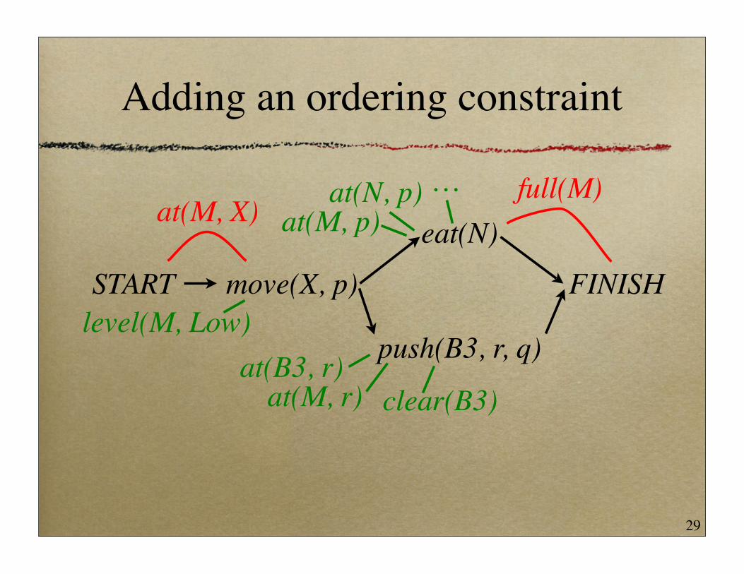
Adding an ordering constraint

START move(X, p)

eat(N)

FINISH

push(B3, r, q)

at(M, X)full(M)at(N, p)

at(M, p)

at(B3, r)level(M, Low)

at(M, r) clear(B3)

…

29

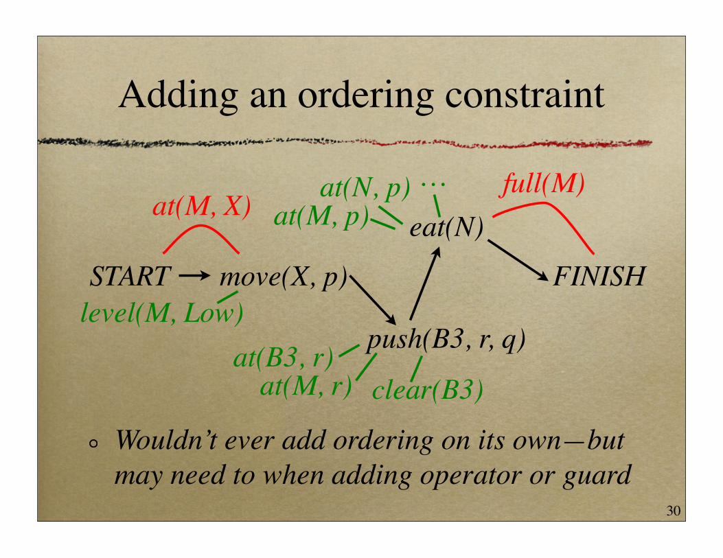
Adding an ordering constraint

START move(X, p)

eat(N)

FINISH

push(B3, r, q)

at(M, X)full(M)

at(M, p)

at(B3, r)at(M, r) clear(B3)

…

Wouldn’t ever add ordering on its own—but may need to when adding operator or guard

level(M, Low)

at(N, p)

30

Adding a guard

START move(X, p)

eat(N)

FINISH

push(B3, r, q)

at(M, X)full(M)at(N, p)

at(M, p)

at(B3, r)level(M, Low)

at(M, r) clear(B3)

…

31

Adding a guard

Must go forward (may need to add ordering)Can’t cross operator that affects condition

START move(X, p)

eat(N)

FINISH

push(B3, r, q)

at(M, X)full(M)at(N, p)

at(M, p)

at(B3, r)level(M, Low)

at(M, r) clear(B3)

…

32

Adding a guard

Might involve binding a variable (may be more than one way to do so)

START move(X, p)

eat(N)

FINISH

push(B3, r, q)

at(M, X)full(M)at(N, W)

at(M, p)

at(B3, r)level(M, Low)

at(M, r) clear(B3)

…

33

Adding an operator

START move(X, p)

eat(N)

FINISH

push(B3, r, q)

at(M, X)full(M)at(N, W)

at(M, p)

at(B3, r)level(M, Low)

at(M, r) clear(B3)

…

34

Adding an operator

START move(X, p)

eat(N)

FINISH

push(B3, r, q)

at(M, X)full(M)at(N, W)

at(M, p)

at(B3, r)level(M, Low)

at(M, r) clear(B3)

…

move(s, r)at(M, s)

level(M, Low)

35

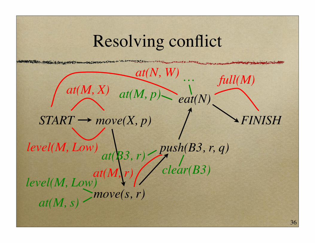
Resolving conflict

START move(X, p)

eat(N)

FINISH

push(B3, r, q)

at(M, X)full(M)at(N, W)

at(M, p)

level(M, Low)

clear(B3)

…

move(s, r)

at(B3, r)at(M, r)

at(M, s)level(M, Low)

36

Recap of neighborhood

Pick an open preconditionPick an operator and binding that can satisfy it

may need to add a new opor can use existing op

Add an ordering constraint and guardResolve conflicts by adding more ordering constraints or bindings

37

Consistency & completeness

Consistency: no cycles in ordering, preconditions guaranteed true throughout guard intervalsCompleteness: no open preconditionsSearch maintains consistency, terminates when complete

38

Execution

A consistent, complete plan can be executed by linearizing itExecute actions in any order that matches the ordering constraintsFill in unbound variables in any consistent way

39

Plan Graphs

40

Planning & model search

For a long time, it was thought that SAT-style model search was a non-starter as a planning algorithmMore recently, people have written fast planners that

propositionalize the domainturn it into a CSP or SAT problemsearch for a model

41

Plan graph

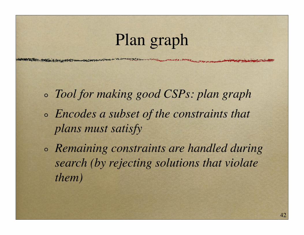
Tool for making good CSPs: plan graphEncodes a subset of the constraints that plans must satisfyRemaining constraints are handled during search (by rejecting solutions that violate them)

42

Example

Start state: have(Cake)Goal: have(Cake) ∧ eaten(Cake)

Operators: bake, eat

43

Operators

Bakepre: ¬have(Cake)

post: have(Cake)Eat

pre: have(Cake)post: ¬have(Cake), eaten(Cake)

44

Propositionalizing

Note: this domain is fully propositionalIf we had a general STRIPS domain, would have to pick a universe and propositionalizeE.g., eat(x) would become eat(Banana), eat(Cake), eat(Fred), …

45

Plan graph

Alternating levels: states and actionsFirst level: initial state

have

¬eaten

46

Plan graph

First action level: all applicable actionsLinked to their preconditions

have

¬eateneat

47

Plan graph

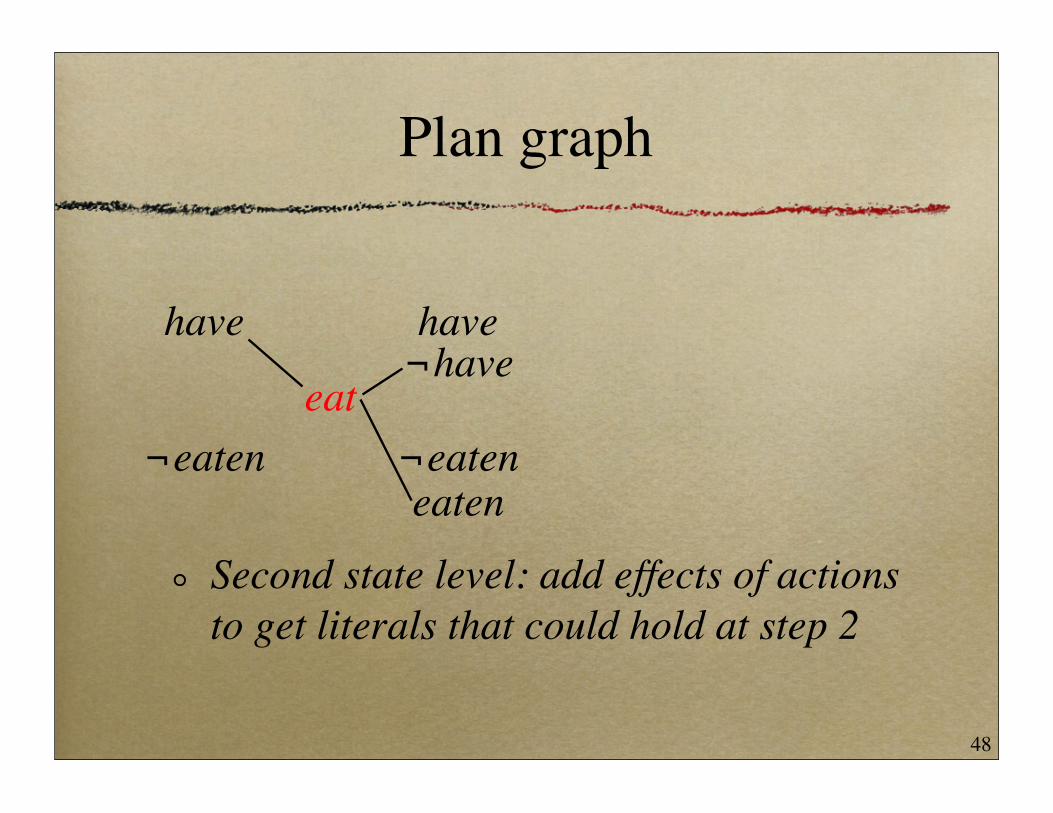
Second state level: add effects of actions to get literals that could hold at step 2

have

¬eateneat

have

¬eateneaten

¬have

48

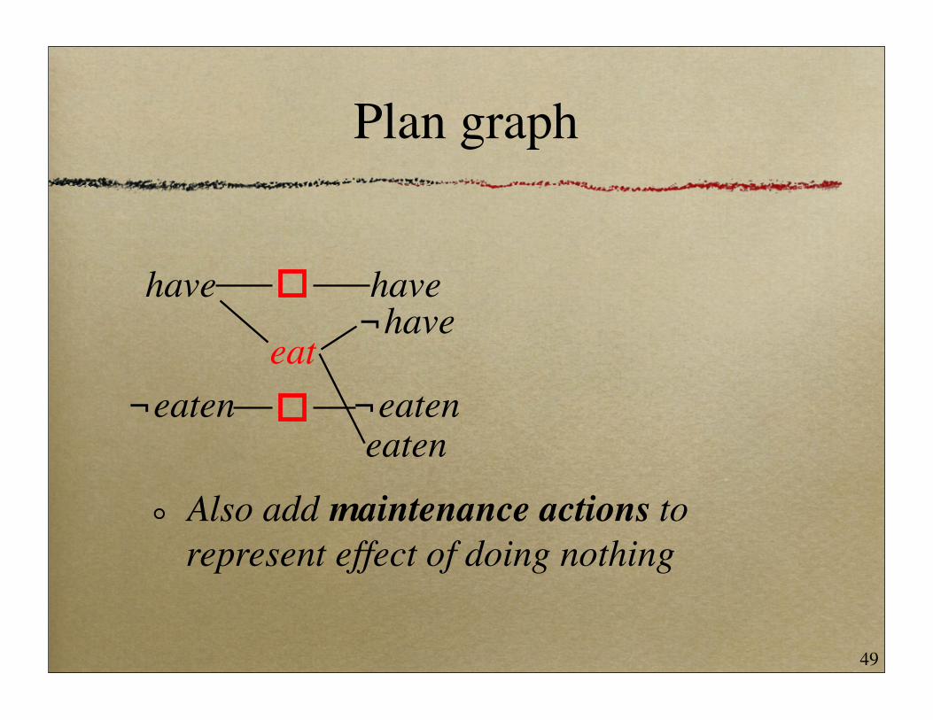
Plan graph

Also add maintenance actions to represent effect of doing nothing

have

¬eateneat

have

¬eateneaten

¬have

49

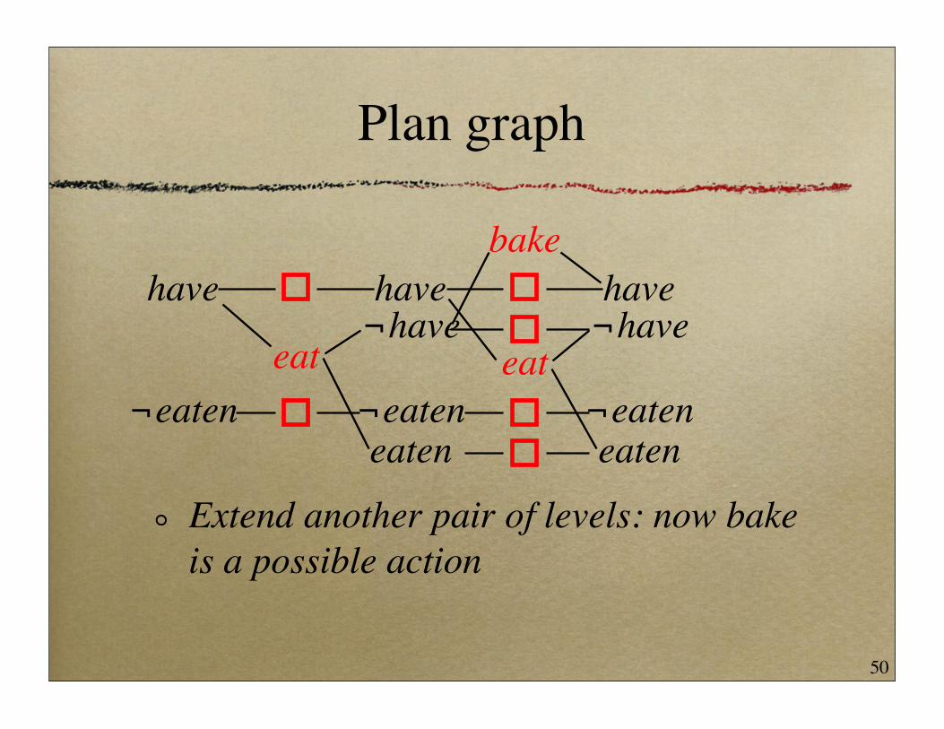
Plan graph

Extend another pair of levels: now bake is a possible action

have

¬eateneat

have

¬eateneaten

¬haveeat

have

¬eateneaten

¬have

bake

50

Plan graph

Can extend as far right as we wantPlan = subset of the actions at each action levelOrdering unspecified within a level

51

Plan graph

In addition to the above links, add mutex links to indicate mutually exclusive actions or literals

have

¬eateneat

have

¬eateneaten

¬haveeat

have

¬eateneaten

¬have

bake

52

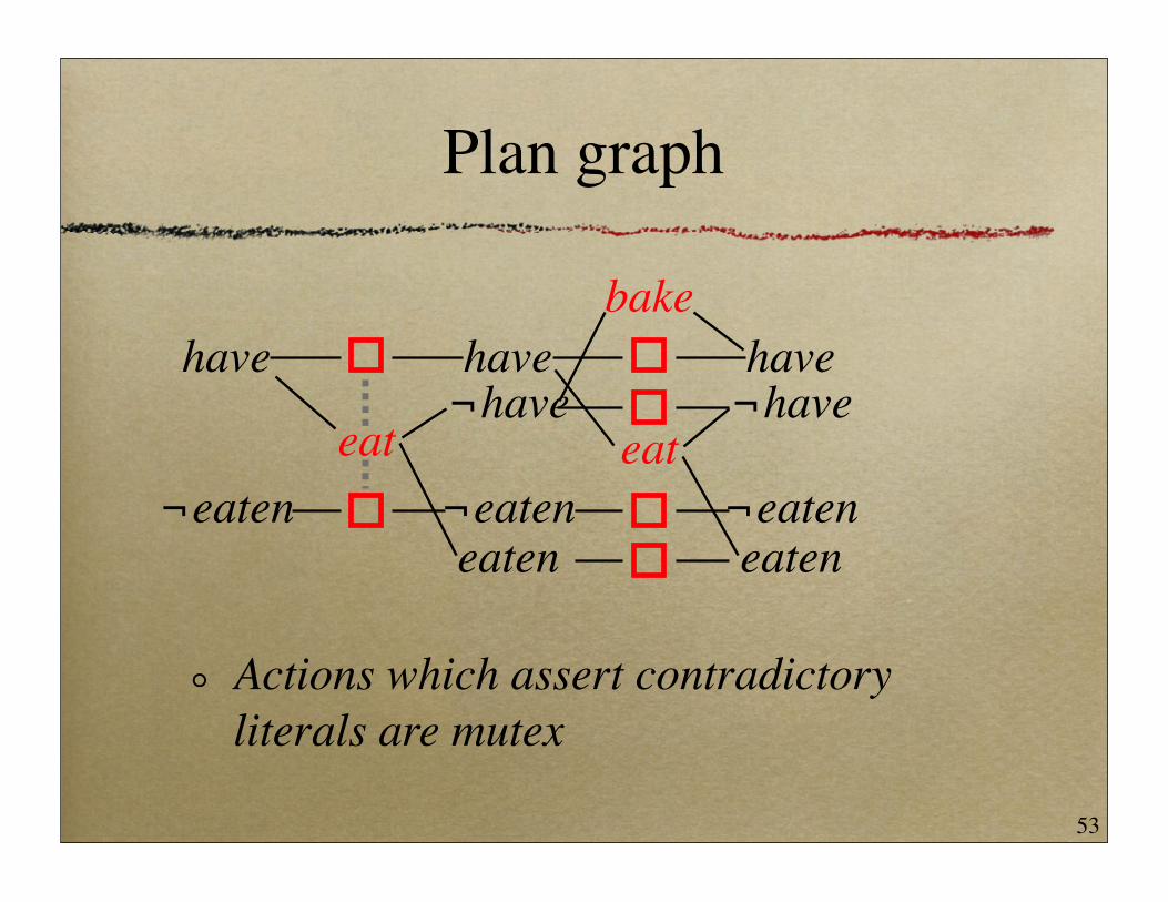
Plan graph

Actions which assert contradictory literals are mutex

have

¬eateneat

have

¬eateneaten

¬haveeat

have

¬eateneaten

¬have

bake

53

Plan graph

Literals are mutex if they are contradictory

have

¬eateneat

have

¬eateneaten

¬haveeat

have

¬eateneaten

¬have

bake

54

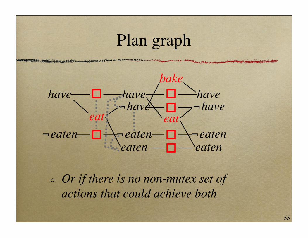
Plan graph

Or if there is no non-mutex set of actions that could achieve both

have

¬eateneat

have

¬eateneaten

¬haveeat

have

¬eateneaten

¬have

bake

55

Plan graph

Actions are also mutex if one deletes a precondition of the other, or if their preconditions are mutex

have

¬eateneat

have

¬eateneaten

¬haveeat

have

¬eateneaten

¬have

bake

56

Getting a plan

Build the plan graph out to some length kTranslate to a SAT formula or CSPSearch for a satisfying assignmentIf found, read off the planIf not, increment k and try againThere is a test to see if k is big enough

57

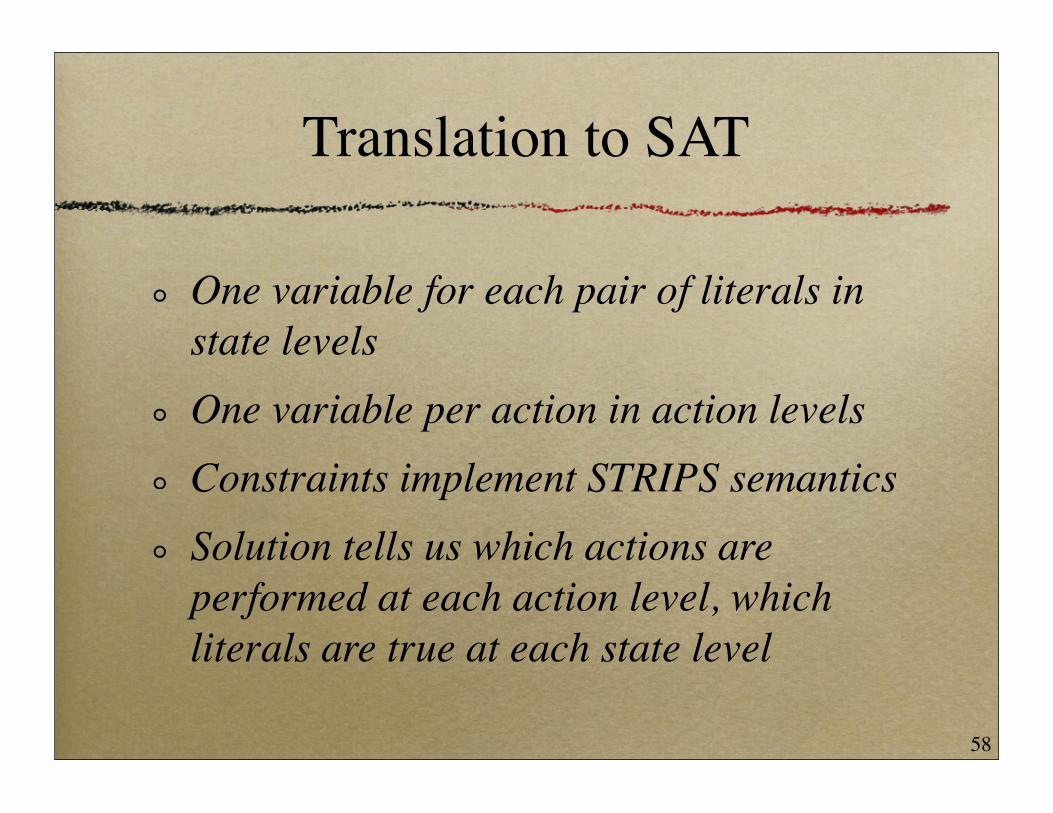
Translation to SAT

One variable for each pair of literals in state levelsOne variable per action in action levelsConstraints implement STRIPS semanticsSolution tells us which actions are performed at each action level, which literals are true at each state level

58

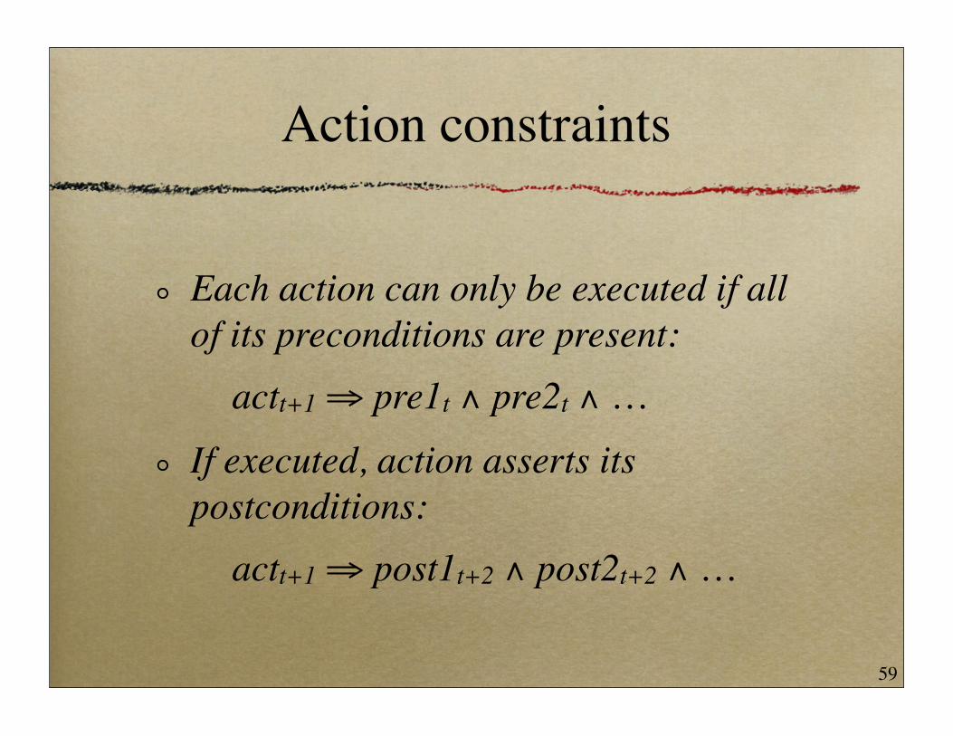
Action constraints

Each action can only be executed if all of its preconditions are present:

actt+1 ⇒ pre1t ∧ pre2t ∧ …

If executed, action asserts its postconditions:

actt+1 ⇒ post1t+2 ∧ post2t+2 ∧ …

59

Literal constraints

In order to achieve a literal, we must execute an action that achieves it

postt+2 ⇒ act1t+1 ∨ act2t+1 ∨ …

Might be a maintenance action

60

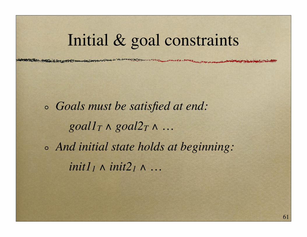
Initial & goal constraints

Goals must be satisfied at end: goal1T ∧ goal2T ∧ …

And initial state holds at beginning:init11 ∧ init21 ∧ …

61

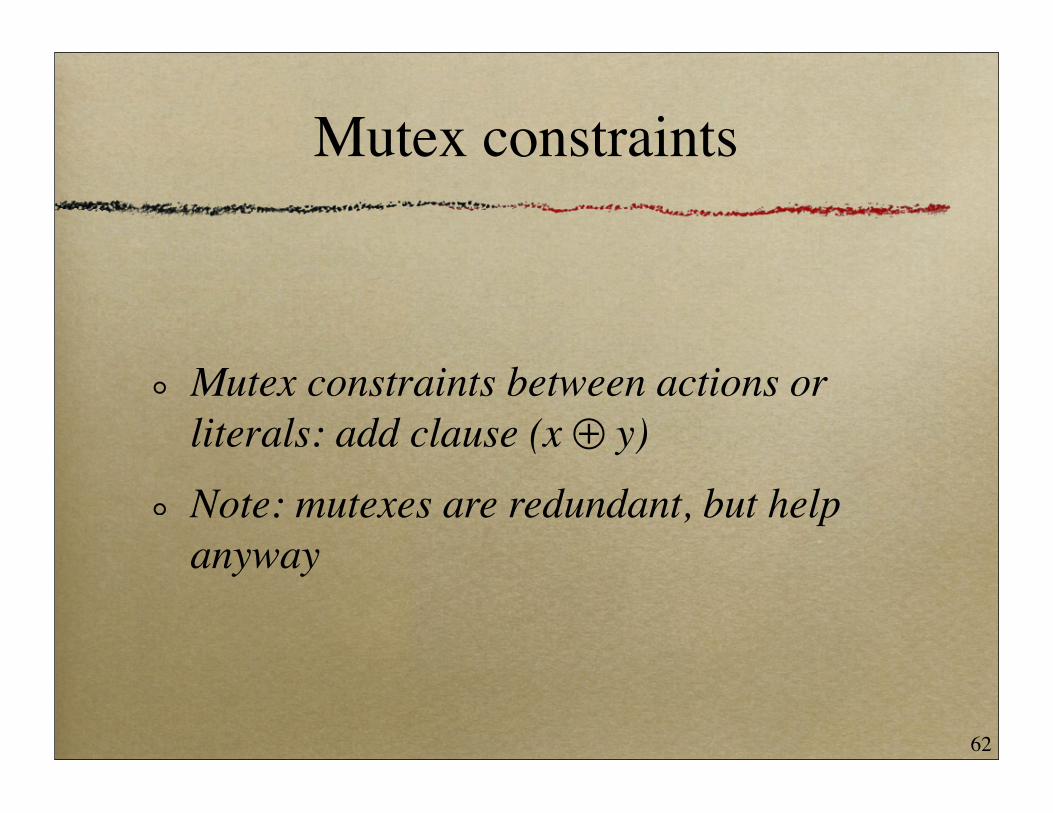
Mutex constraints

Mutex constraints between actions or literals: add clause (x ⊕ y)

Note: mutexes are redundant, but help anyway

62

Plan search

Hand problem to SAT solverOr, simple DFS: start from last level, fill in last action set, compute necessary preconditions, fill in 2nd-to-last action set, etc.If at some level there is no way to do any actions, or no way to fill in consistent preconditions, backtrack

63

Plan search

have

¬eateneat

have

¬eateneaten

¬haveeat

have

¬eateneaten

¬have

bake

64

Optimization and Search

65

Search problem

Typical search problem: CSP or SATDescription: variables, domains, constraintsFind a solution that satisfies constraintsAny satisfying solution is OK

66

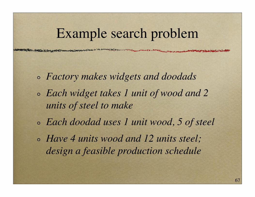
Example search problem

Factory makes widgets and doodadsEach widget takes 1 unit of wood and 2 units of steel to makeEach doodad uses 1 unit wood, 5 of steelHave 4 units wood and 12 units steel; design a feasible production schedule

67

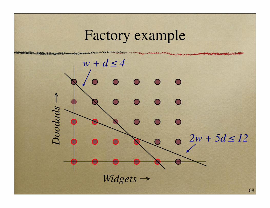
Factory example

Widgets →

Doo

dads

→w + d ≤ 4

2w + 5d ≤ 12

68

Optimization

Not all feasible solutions are equally goodWithin feasible set, want to optimize an objective functionE.g., maximize profit:

Each widget yields a profit of $1Each doodad nets $2

69

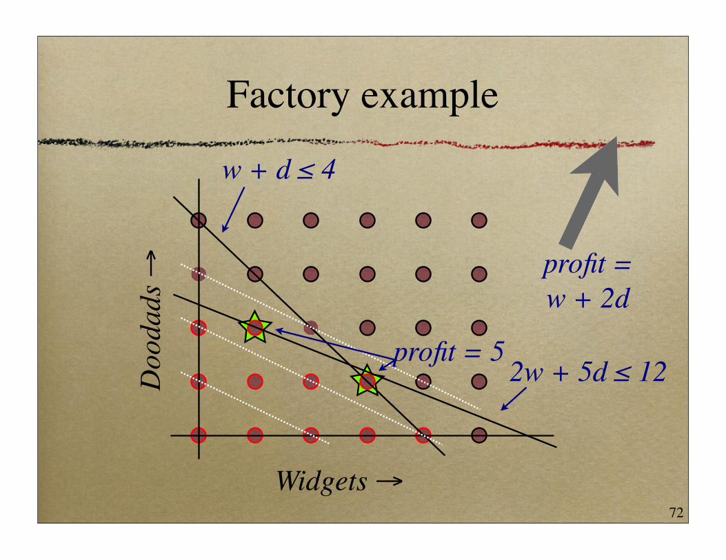
Factory example

Widgets →

Doo

dads

→w + d ≤ 4

2w + 5d ≤ 12

profit = w + 2d

70

Factory example

Widgets →

Doo

dads

→w + d ≤ 4

2w + 5d ≤ 12

profit = w + 2d

71

Factory example

Widgets →

Doo

dads

→w + d ≤ 4

2w + 5d ≤ 12

profit = w + 2d

profit = 5

72

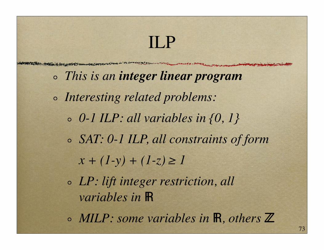
ILP

This is an integer linear programInteresting related problems:

0-1 ILP: all variables in {0, 1}SAT: 0-1 ILP, all constraints of formx + (1-y) + (1-z) ≥ 1LP: lift integer restriction, all variables in ℝMILP: some variables in ℝ, others ℤ

73

Search

Can still use search algorithms like DFID for optimization problemsJust remember the best objective value seen so farThis is a fine algorithm, but we can often do better!

74

Bounds

75

Smarter algorithms

We can build smarter algorithms by remembering bounds on optimal valueFirst idea: if we have a solution with profit 3, add a constraint “profit ≥ 3”If we then find a solution with profit 5, replace constraint with “profit ≥ 5”

76

Factory example

Widgets →

Doo

dads

→w + d ≤ 4

2w + 5d ≤ 12

profit = w + 2d

77

Factory example

Widgets →

Doo

dads

→w + d ≤ 4

2w + 5d ≤ 12

profit = w + 2d

78

Factory example

Widgets →

Doo

dads

→w + d ≤ 4

2w + 5d ≤ 12

profit = w + 2d

79

Factory example

Widgets →

Doo

dads

→w + d ≤ 4

2w + 5d ≤ 12

profit = w + 2d

80

Factory example

Widgets →

Doo

dads

→w + d ≤ 4

2w + 5d ≤ 12

profit = w + 2d

81

Upper bounds

Suppose we’re partway finished: examined a few nodes and found a solution

82

Factory example

Widgets →

Doo

dads

→w + d ≤ 4

2w + 5d ≤ 12

profit = w + 2d

83

Upper bounds

Have a solution of profit $4How much profit would we lose by stopping now?Might we find a node with profit $73 if we kept looking?

84

Relaxation

Idea: what if we solve an easier version of the problem?If we make feasible region bigger, objective value can only get betterBigger feasible region = relaxationValue of relaxed problem is an upper bound on value of original problem

85

LP relaxation

Nice way of making feasible region bigger: drop integrality constraintsCalled the LP relaxation of our problemLPs are efficiently solvable (see below)

86

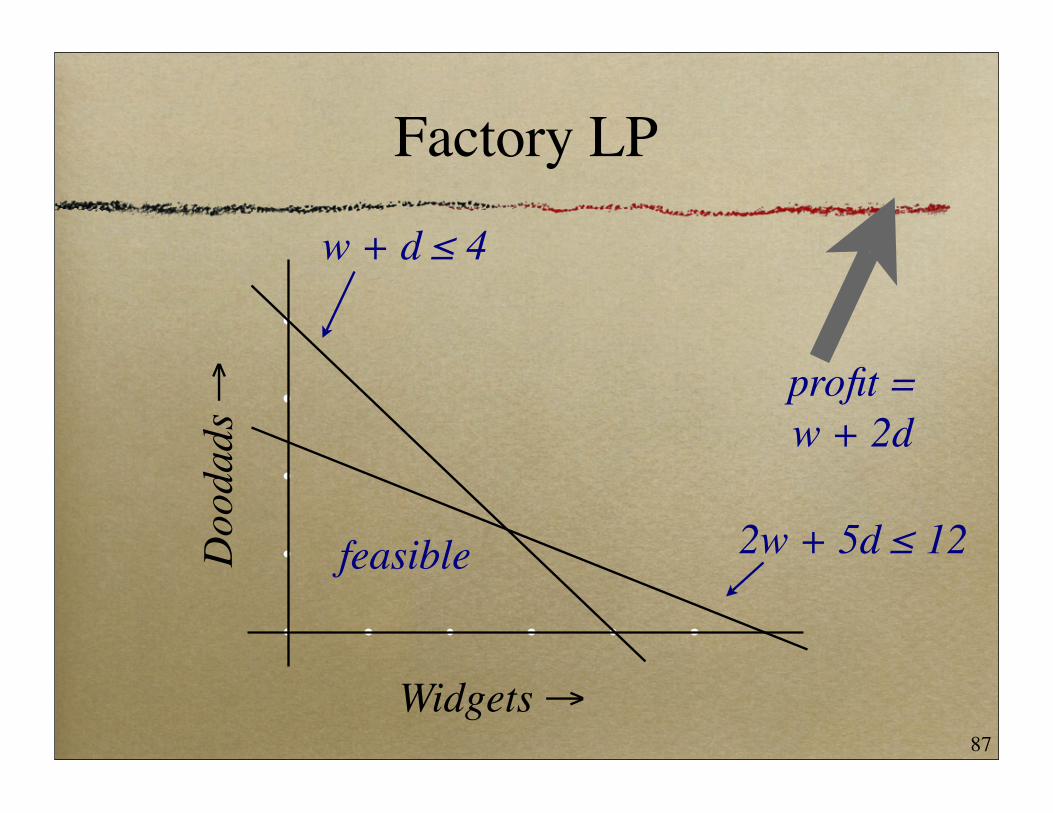
Factory LP

Widgets →

Doo

dads

→

feasible

w + d ≤ 4

2w + 5d ≤ 12

profit = w + 2d

87

profit = 5 1/3

Factory LP

Widgets →

Doo

dads

→

feasible

w + d ≤ 4

2w + 5d ≤ 12

profit = w + 2d

88

Upper bounds

So, we have a solution of profit $4And we know the best solution has profit no more than $5 1/3If we’re lazy, we can stop now

89

More bounds

90

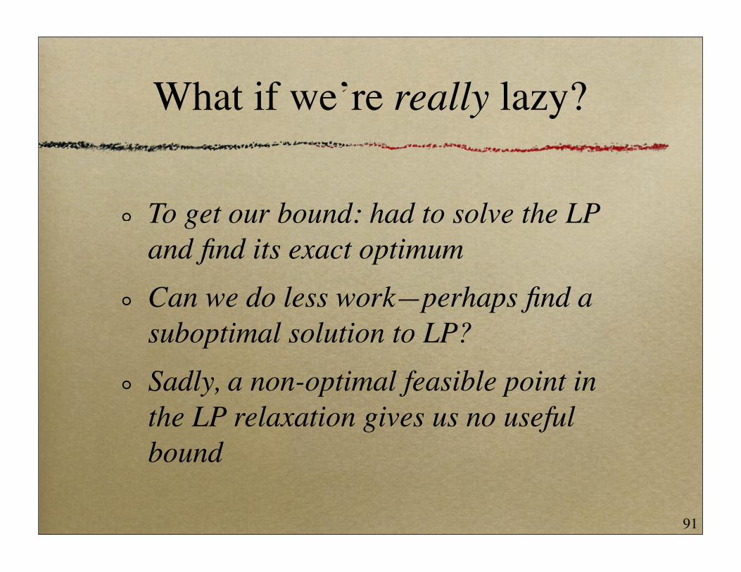
What if we’re really lazy?

To get our bound: had to solve the LP and find its exact optimumCan we do less work—perhaps find a suboptimal solution to LP?Sadly, a non-optimal feasible point in the LP relaxation gives us no useful bound

91

A simple bound

Recall: constraint w + d ≤ 4 (limit on wood)profit w + 2d

Since w, d ≥ 0, profit = w + 2d ≤ 2w + 2d

And, doubling both sides of constraint,2w + 2d ≤ 8 ⇒ profit ≤ 8

92

The same trick works twice

Try other constraint (steel use)2w + 5d ≤ 12

2*profit = 2w + 4d ≤ 2w + 5d ≤ 12So profit ≤ 6

93

In fact it works infinitely often

Could take any positive-weight linear combination of our constraints

negative weights would flip sign

a (w + d – 4) + b (2w + 5d – 12) ≤ 0(a + 2b) w + (a + 5b) d ≤ 4a + 12b

94

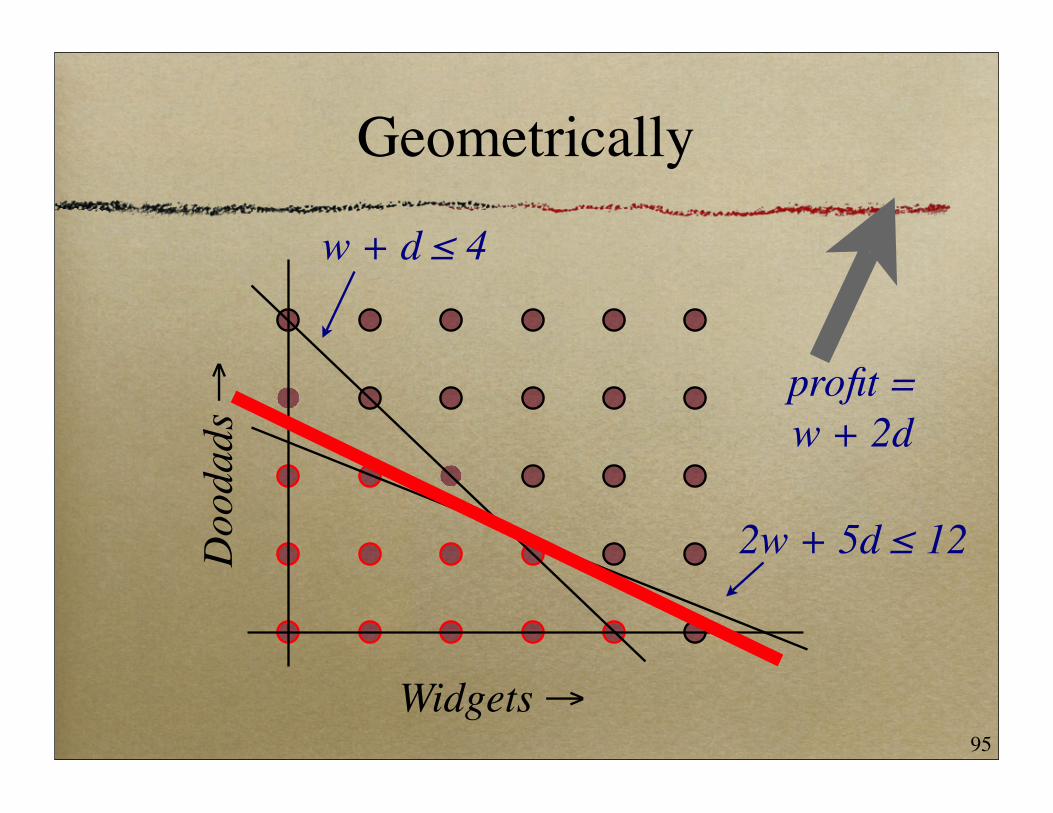
Geometrically

Widgets →

Doo

dads

→w + d ≤ 4

2w + 5d ≤ 12

profit = w + 2d

95

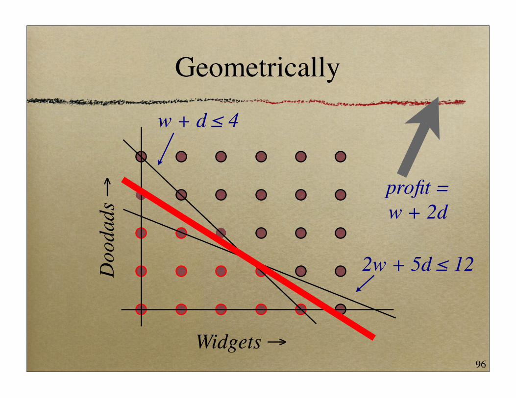
Geometrically

Widgets →

Doo

dads

→w + d ≤ 4

2w + 5d ≤ 12

profit = w + 2d

96

Geometrically

Widgets →

Doo

dads

→w + d ≤ 4

2w + 5d ≤ 12

profit = w + 2d

97

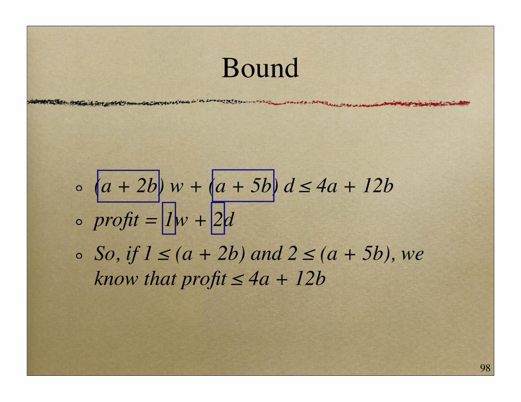
Bound

(a + 2b) w + (a + 5b) d ≤ 4a + 12bprofit = 1w + 2dSo, if 1 ≤ (a + 2b) and 2 ≤ (a + 5b), we know that profit ≤ 4a + 12b

98

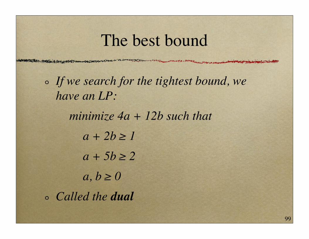
The best bound

If we search for the tightest bound, we have an LP:

minimize 4a + 12b such thata + 2b ≥ 1a + 5b ≥ 2a, b ≥ 0

Called the dual99

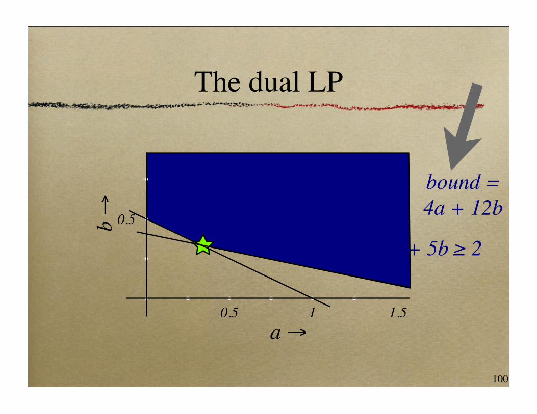
The dual LP

a →

b → a = b = 1/3

a + 2b ≥ 1

a + 5b ≥ 2

0.5

0.5

1 1.5

bound = 4a + 12b

feasible

100

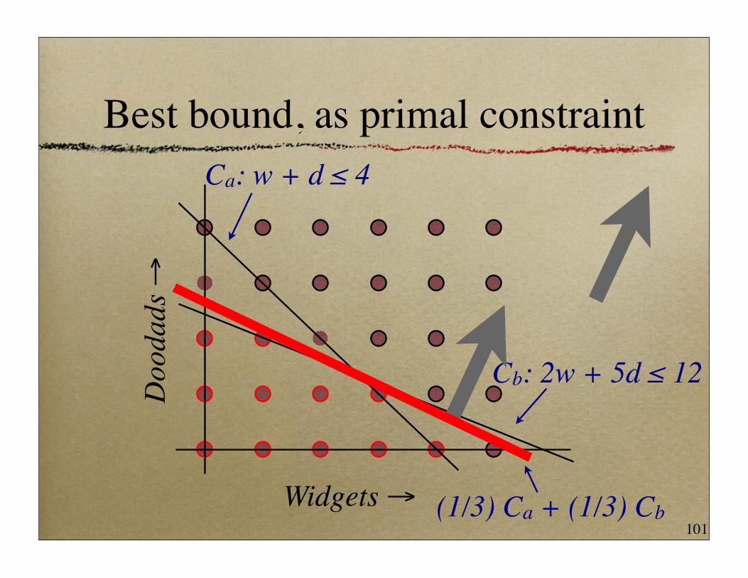
Best bound, as primal constraint

Widgets →

Doo

dads

→Ca: w + d ≤ 4

Cb: 2w + 5d ≤ 12

(1/3) Ca + (1/3) Cb101

Bound from dual

a = b = 1/3 yields bound of 4a + 12b = 16/3 = 5 1/3

Same as bound from original relaxation!No accident: dual of an LP always* has same objective value

102

So why bother?

Reason 1: any feasible solution to dual yields upper bound (compared with only optimal solution to primal)Reason 2: dual might be easier to work with

103

Recap

Each feasible point of dual is an upper bound on objectiveEach feasible point of primal is a lower bound on objective

for ILP, each integral feasible point

104

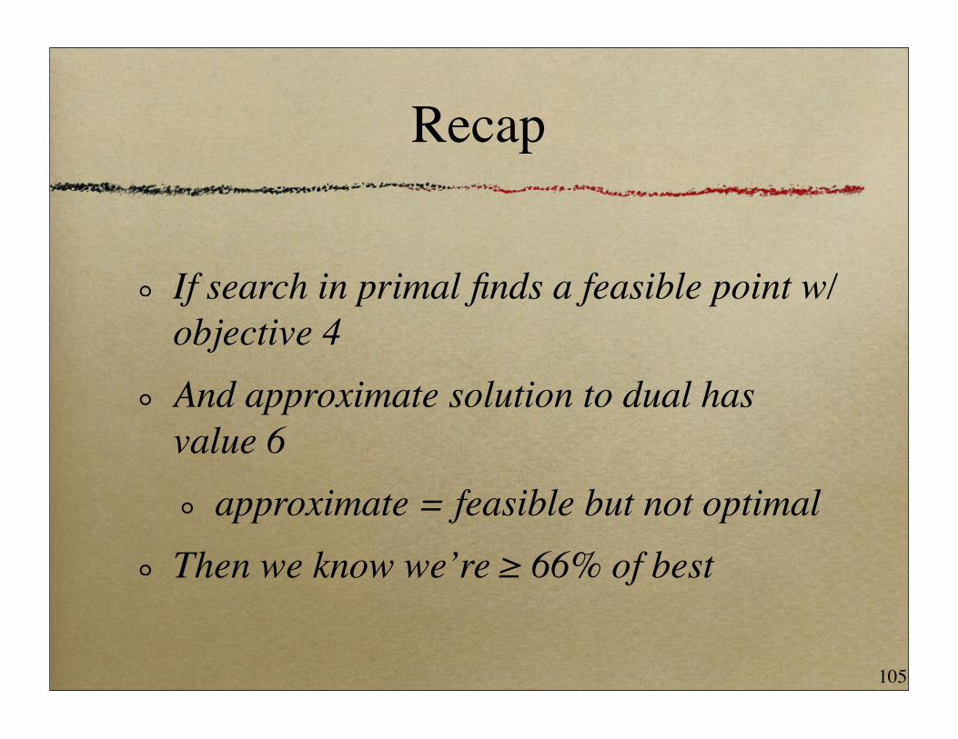
Recap

If search in primal finds a feasible point w/ objective 4And approximate solution to dual has value 6

approximate = feasible but not optimalThen we know we’re ≥ 66% of best

105

More about the dual

106

Dual dual

Take the dual of an LP twice, get the original LP back (called primal)Many LP solvers will give you both primal and dual solutions at the same time for no extra cost

107

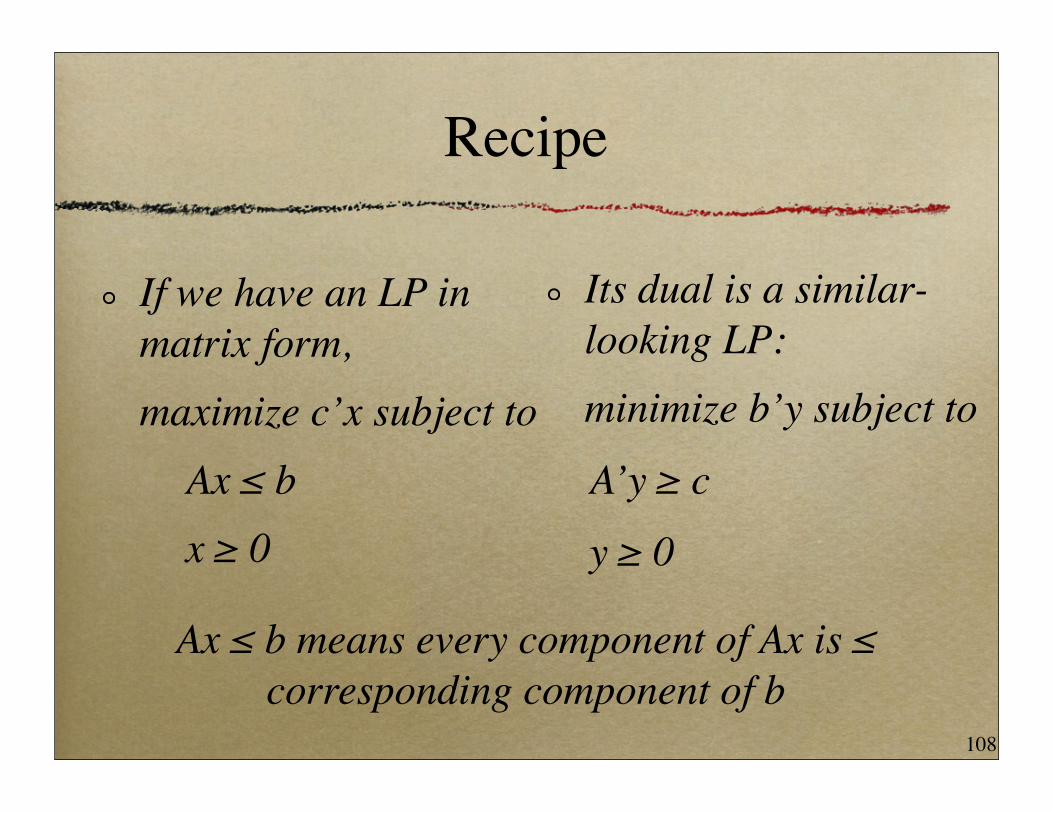
Recipe

If we have an LP in matrix form,maximize c’x subject to

Ax ≤ bx ≥ 0

Its dual is a similar-looking LP:minimize b’y subject to

A’y ≥ c

y ≥ 0

Ax ≤ b means every component of Ax is ≤ corresponding component of b

108

Recipe with equalities

If we have an LP with equalities,maximize c’x s.t.

Ax ≤ bEx = fx ≥ 0

Its dual has some unrestricted variables:

minimize b’y + f’z s.t.

A’y + E’z ≥ c

y ≥ 0

z unrestricted

109

Interpreting the dual variables

The primal variable variables in the factory LP were how many widgets and doodads to produceWe interpreted dual variables as multipliers for primal constraints

110

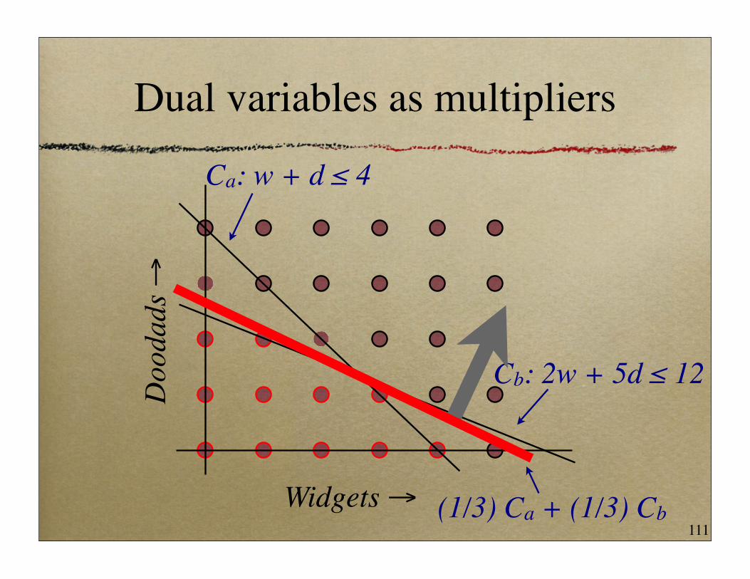
Dual variables as multipliers

Widgets →

Doo

dads

→Ca: w + d ≤ 4

Cb: 2w + 5d ≤ 12

(1/3) Ca + (1/3) Cb111

Dual variables as prices

“Multiplier” interpretation doesn’t give much intuitionIt is often possible to interpret dual variables as prices for primal constraints

112

Dual variables as prices

Suppose someone offered us a quantity ε of wood, loosening constraint to

w + d ≤ 4 + ε

How much should we be willing to pay for this wood?

113

Dual variables as prices

RHS in primal is objective in dualSo, dual constraints stay same, previous solution a = b = 1/3 still dual feasible

still optimal if ε small enough

Bound changes to (4 + ε) a + 12 b, difference of ε * 1/3So we should pay up to $1/3 per unit of wood (in small quantities)

114

Duality example

115

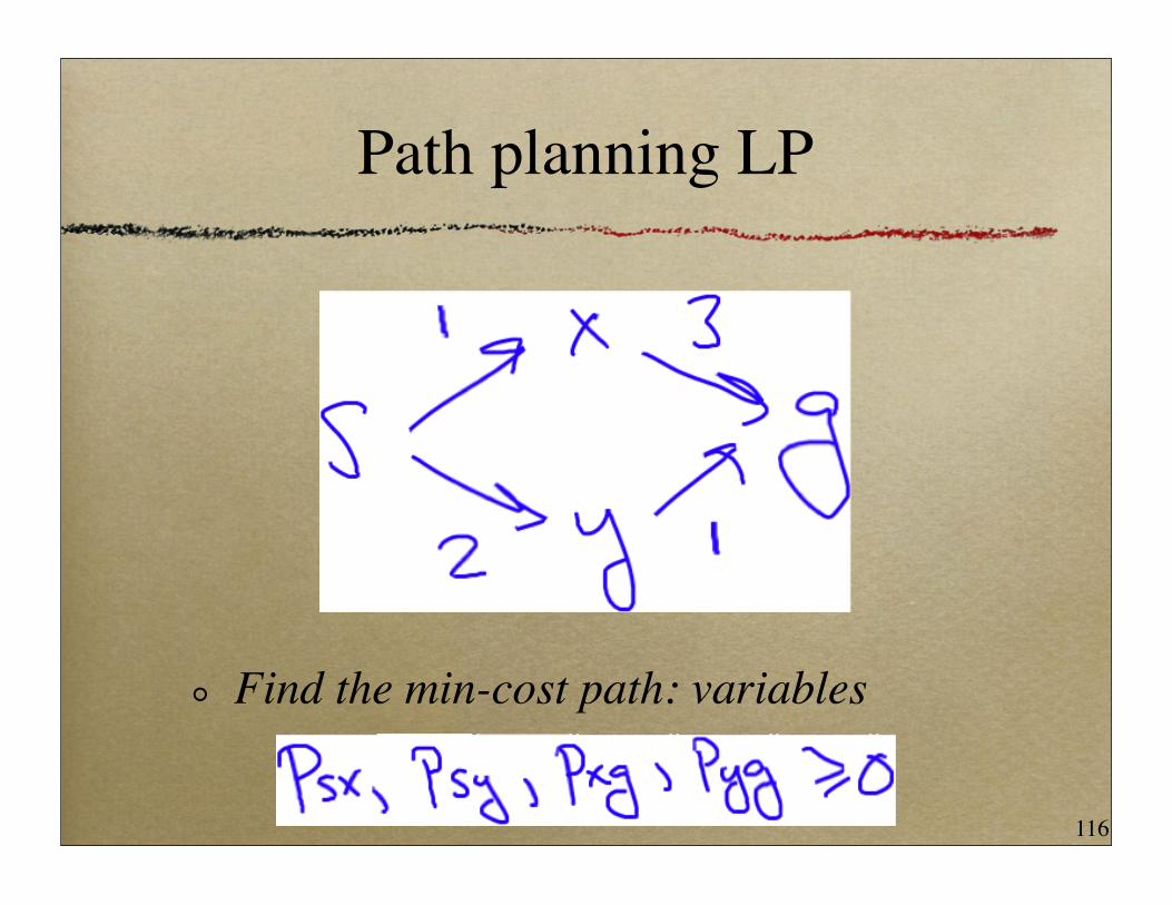
Path planning LP

Find the min-cost path: variables

116

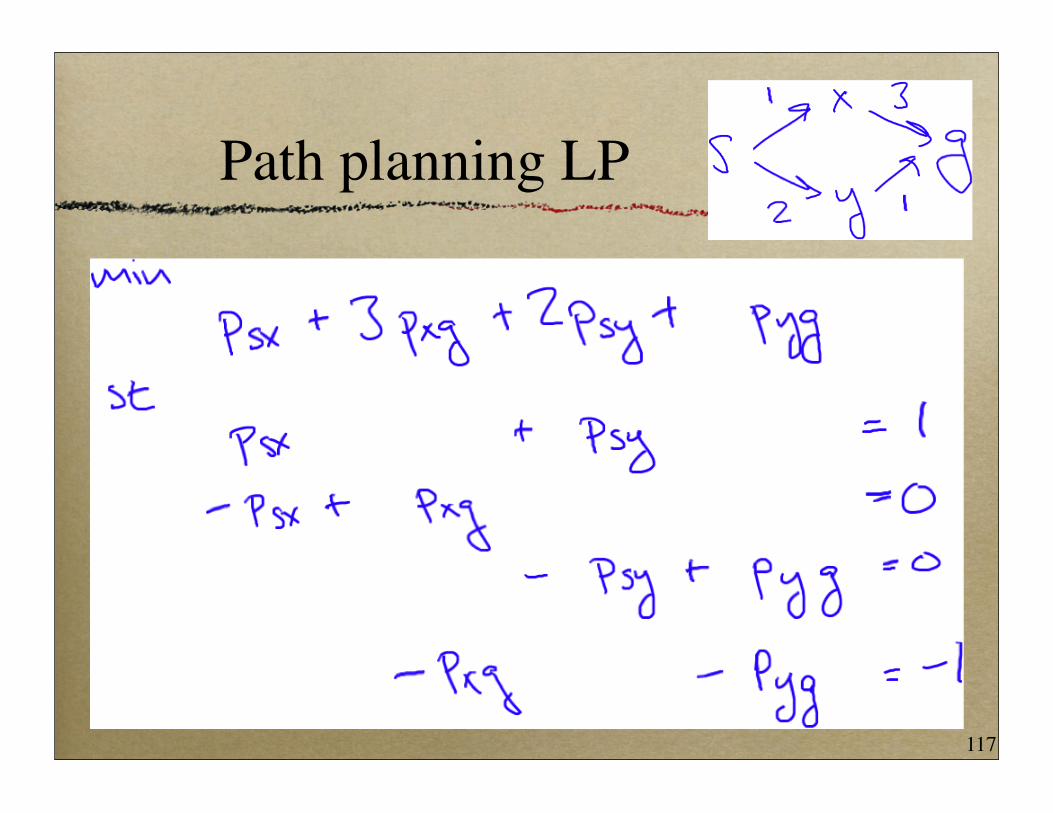
Path planning LP

117

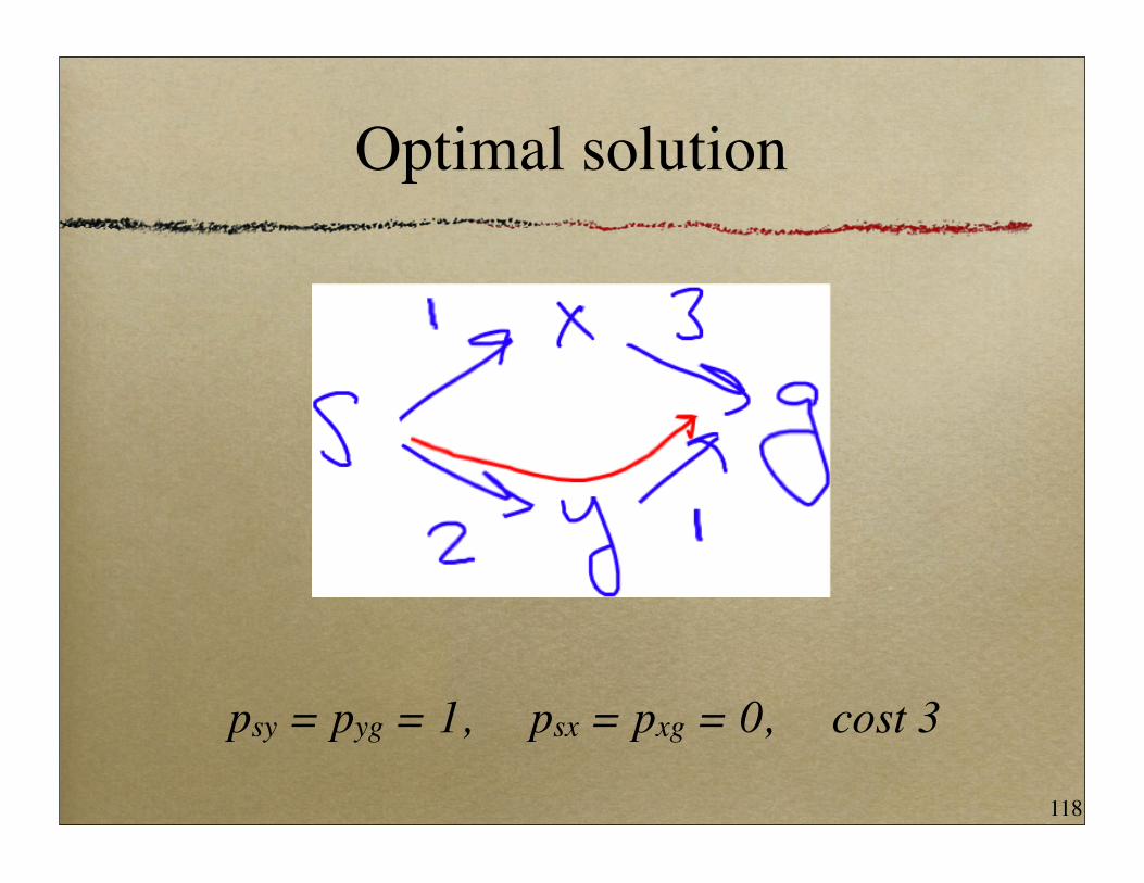
Optimal solution

psy = pyg = 1, psx = pxg = 0, cost 3

118

Matrix form

119

Dual

120

Dual objective

To get tightest bound, maximize:

121

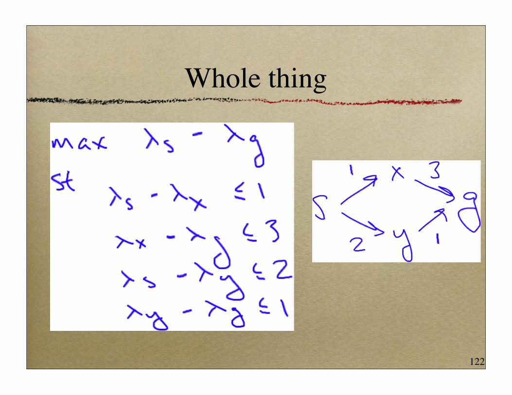
Whole thing

122