Embed Size (px)
Citation preview
15-744: Computer Networking
L-4 Routers
L -4; 1-28-01© Srinivasan Seshan, 2002 2
Routing
• How do routers process IP packets• Forwarding lookup algorithms• Assigned reading
• [D+97] Small Forwarding Tables for Fast Routing Lookups
L -4; 1-28-01© Srinivasan Seshan, 2002 3
Forwarding vs. Routing
• Forwarding: the process of moving packets from input to output• The forwarding table• Information in the packet
• Routing: process by which the forwarding table is built and maintained• One or more routing protocols• Procedures (algorithms) to convert routing info to
forwarding table.
L -4; 1-28-01© Srinivasan Seshan, 2002 4
Outline
• Alternative methods for packet forwarding
• IP packet routing
• Variable prefix match
• Packet classification
L -4; 1-28-01© Srinivasan Seshan, 2002 5
Techniques for Forwarding Packets
• Source routing• Packet carries path
• Table of virtual circuits• Connection routed through network to setup
state• Packets forwarded using connection state
• Table of global addresses (IP)• Routers keep next hop for destination• Packets carry destination address
L -4; 1-28-01© Srinivasan Seshan, 2002 6
Source Routing
• List entire path in packet• Driving directions (north 3 hops, east, etc..)
• Router processing• Examine first step in directions• Strip first step from packet• Forward to step just stripped off
L -4; 1-28-01© Srinivasan Seshan, 2002 7
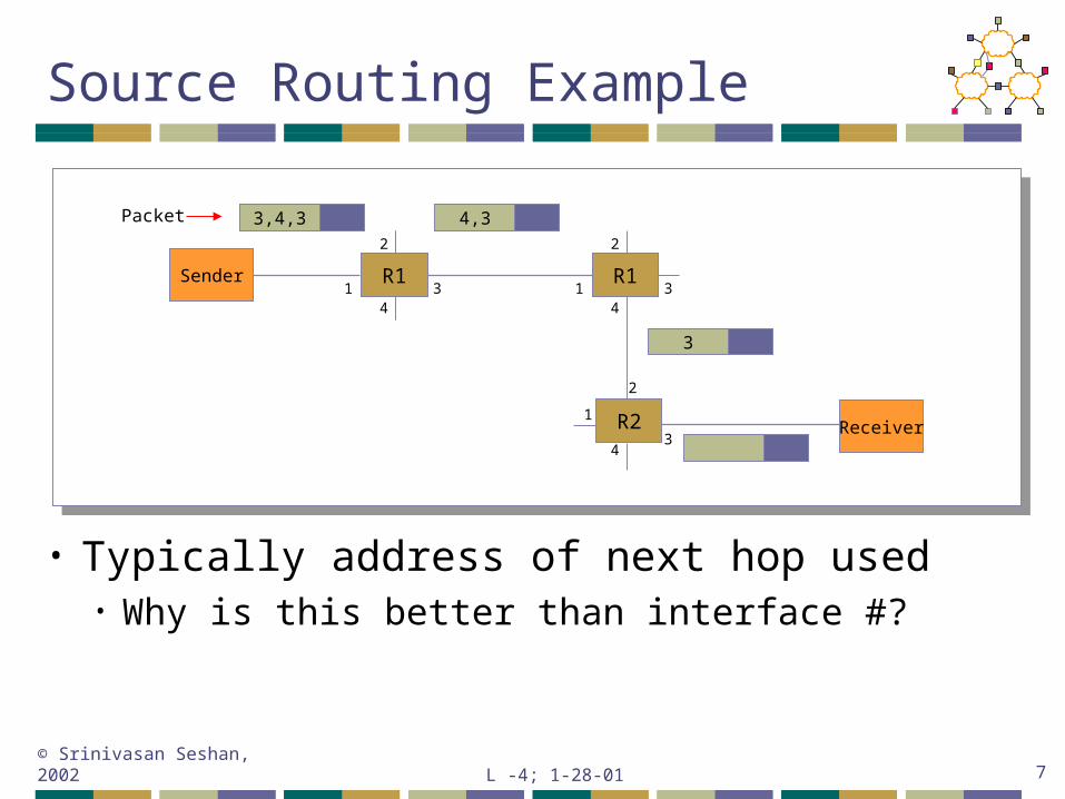
Source Routing Example
Receiver
Packet 3,4,3
Sender
2
34
1
2
34
1
2
34
1
R1
R2
R1
4,3
3
• Typically address of next hop used• Why is this better than interface #?
L -4; 1-28-01© Srinivasan Seshan, 2002 8
Source Routing
• Advantages• Switches can be very simple and fast
• Disadvantages• Variable (unbounded) header size• Sources must know or discover topology (e.g.,
failures)
• Typical use• Ad-hoc networks (DSR)• Machine room networks (Myrinet)
L -4; 1-28-01© Srinivasan Seshan, 2002 9
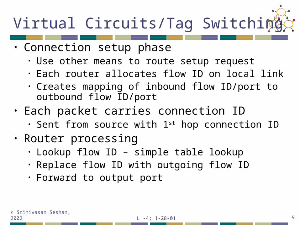
Virtual Circuits/Tag Switching
• Connection setup phase• Use other means to route setup request • Each router allocates flow ID on local link• Creates mapping of inbound flow ID/port to outbound
flow ID/port• Each packet carries connection ID
• Sent from source with 1st hop connection ID• Router processing
• Lookup flow ID – simple table lookup• Replace flow ID with outgoing flow ID• Forward to output port
L -4; 1-28-01© Srinivasan Seshan, 2002 10
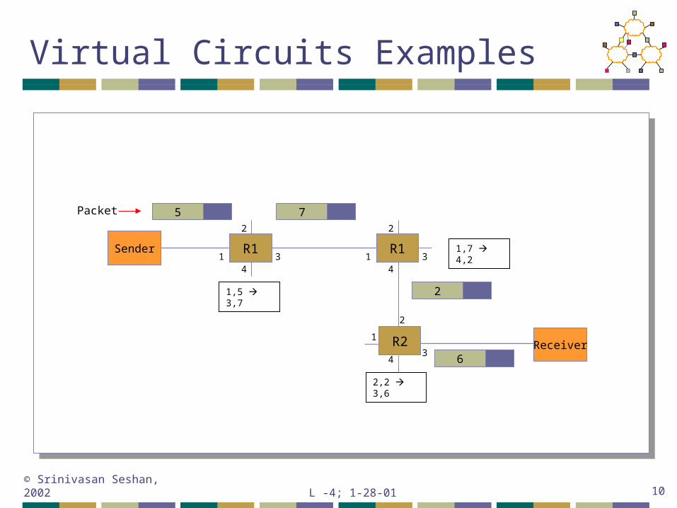
Virtual Circuits Examples
Receiver
Packet
1,5 3,7
Sender
2
34
11,7 4,2
2
34
1
2
34
1
2,2 3,6
R1
R2
R1
5 7
2
6
L -4; 1-28-01© Srinivasan Seshan, 2002 11
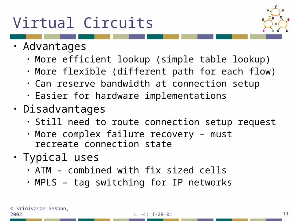
Virtual Circuits
• Advantages• More efficient lookup (simple table lookup)• More flexible (different path for each flow)• Can reserve bandwidth at connection setup• Easier for hardware implementations
• Disadvantages• Still need to route connection setup request• More complex failure recovery – must recreate
connection state• Typical uses
• ATM – combined with fix sized cells• MPLS – tag switching for IP networks
L -4; 1-28-01© Srinivasan Seshan, 2002 12
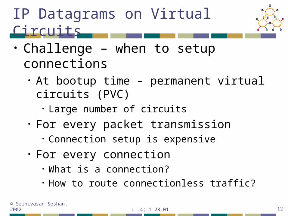
IP Datagrams on Virtual Circuits
• Challenge – when to setup connections• At bootup time – permanent virtual circuits
(PVC)• Large number of circuits
• For every packet transmission• Connection setup is expensive
• For every connection• What is a connection?• How to route connectionless traffic?
L -4; 1-28-01© Srinivasan Seshan, 2002 13
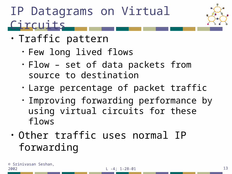
IP Datagrams on Virtual Circuits
• Traffic pattern• Few long lived flows• Flow – set of data packets from source to
destination• Large percentage of packet traffic• Improving forwarding performance by using
virtual circuits for these flows
• Other traffic uses normal IP forwarding
L -4; 1-28-01© Srinivasan Seshan, 2002 14
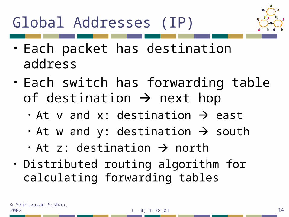
Global Addresses (IP)
• Each packet has destination address• Each switch has forwarding table of
destination next hop• At v and x: destination east• At w and y: destination south• At z: destination north
• Distributed routing algorithm for calculating forwarding tables
L -4; 1-28-01© Srinivasan Seshan, 2002 15
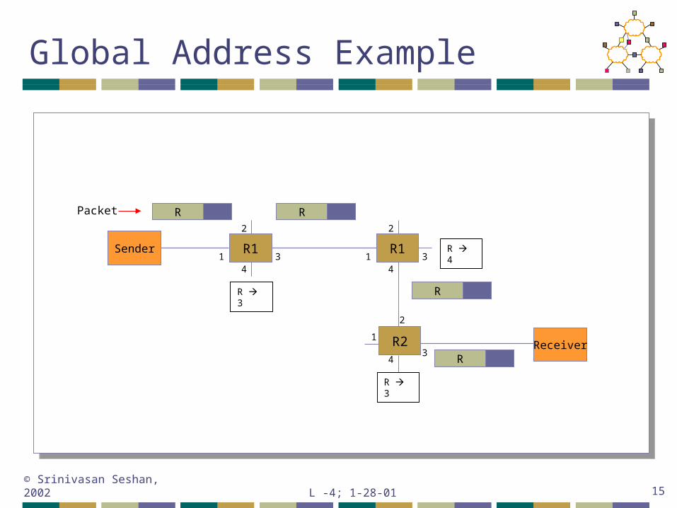
Global Address Example
Receiver
Packet R
Sender
2
34
1
2
34
1
2
34
1
R1
R2
R1
R
RR 3
R 4
R 3
R
L -4; 1-28-01© Srinivasan Seshan, 2002 16
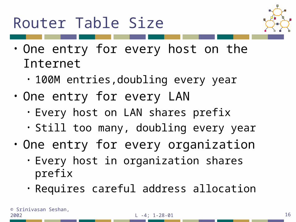
Router Table Size
• One entry for every host on the Internet• 100M entries,doubling every year
• One entry for every LAN• Every host on LAN shares prefix• Still too many, doubling every year
• One entry for every organization• Every host in organization shares prefix• Requires careful address allocation
L -4; 1-28-01© Srinivasan Seshan, 2002 17
Outline
• Alternative methods for packet forwarding
• IP packet routing
• Variable prefix match
• Packet classification
L -4; 1-28-01© Srinivasan Seshan, 2002 18
Original IP Route Lookup
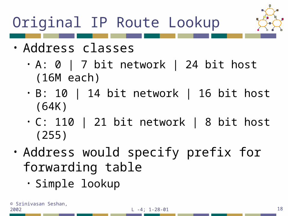
• Address classes• A: 0 | 7 bit network | 24 bit host (16M each)• B: 10 | 14 bit network | 16 bit host (64K)• C: 110 | 21 bit network | 8 bit host (255)
• Address would specify prefix for forwarding table• Simple lookup
L -4; 1-28-01© Srinivasan Seshan, 2002 19
Original IP Route Lookup – Example
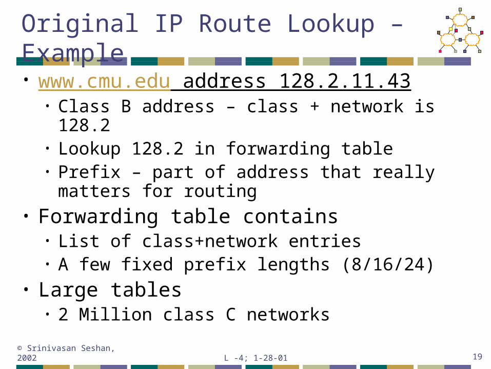
• www.cmu.edu address 128.2.11.43• Class B address – class + network is 128.2• Lookup 128.2 in forwarding table• Prefix – part of address that really matters for
routing• Forwarding table contains
• List of class+network entries• A few fixed prefix lengths (8/16/24)
• Large tables• 2 Million class C networks
L -4; 1-28-01© Srinivasan Seshan, 2002 20
CIDR Revisited
• Supernets• Assign adjacent net addresses to same org• Classless routing (CIDR)
• How does this help routing table?• Combine routing table entries whenever all
nodes with same prefix share same hop
L -4; 1-28-01© Srinivasan Seshan, 2002 21
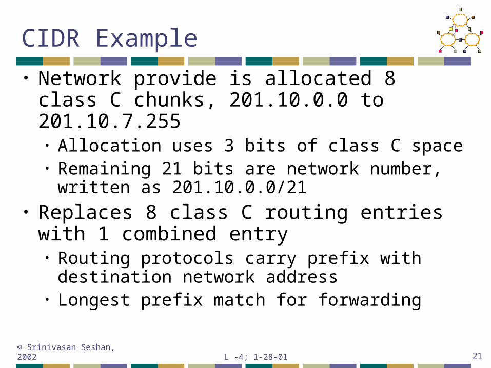
CIDR Example
• Network provide is allocated 8 class C chunks, 201.10.0.0 to 201.10.7.255• Allocation uses 3 bits of class C space• Remaining 21 bits are network number, written
as 201.10.0.0/21• Replaces 8 class C routing entries with 1
combined entry• Routing protocols carry prefix with destination
network address• Longest prefix match for forwarding
L -4; 1-28-01© Srinivasan Seshan, 2002 22
CIDR Illustration
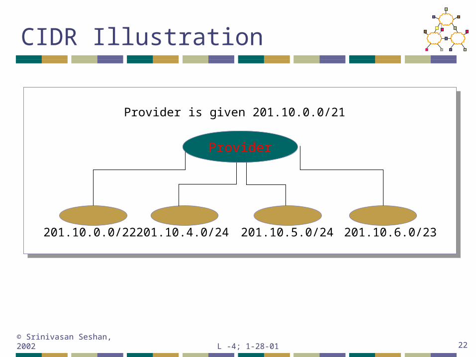
Provider is given 201.10.0.0/21
201.10.0.0/22 201.10.4.0/24 201.10.5.0/24 201.10.6.0/23
Provider
L -4; 1-28-01© Srinivasan Seshan, 2002 23
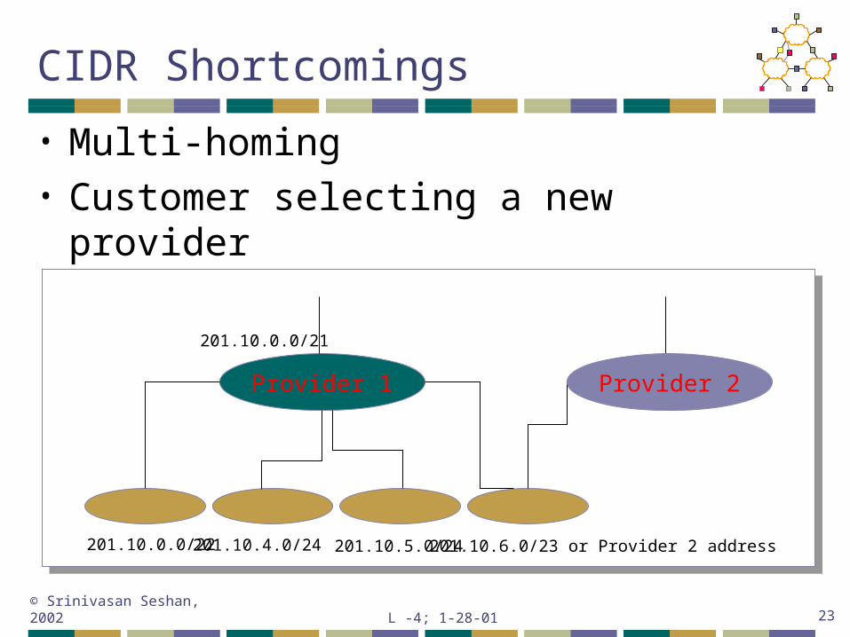
CIDR Shortcomings
• Multi-homing• Customer selecting a new provider
201.10.0.0/21
201.10.0.0/22 201.10.4.0/24 201.10.5.0/24 201.10.6.0/23 or Provider 2 address
Provider 1 Provider 2
L -4; 1-28-01© Srinivasan Seshan, 2002 24
Routing to the Network
H2
H3
H4
R1
10.1.1/24
10.1.1.210.1.1.4
Provider10.1/16 10.1.8/24
10.1.0/24
10.1.1.3
10.1.2/23
R2
10.1.0.2
10.1.8.4
10.1.0.110.1.1.110.1.2.2
10.1.8.110.1.2.110.1.16.1
H1
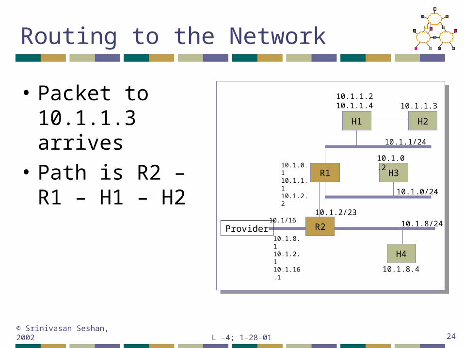
• Packet to 10.1.1.3 arrives
• Path is R2 – R1 – H1 – H2
L -4; 1-28-01© Srinivasan Seshan, 2002 25
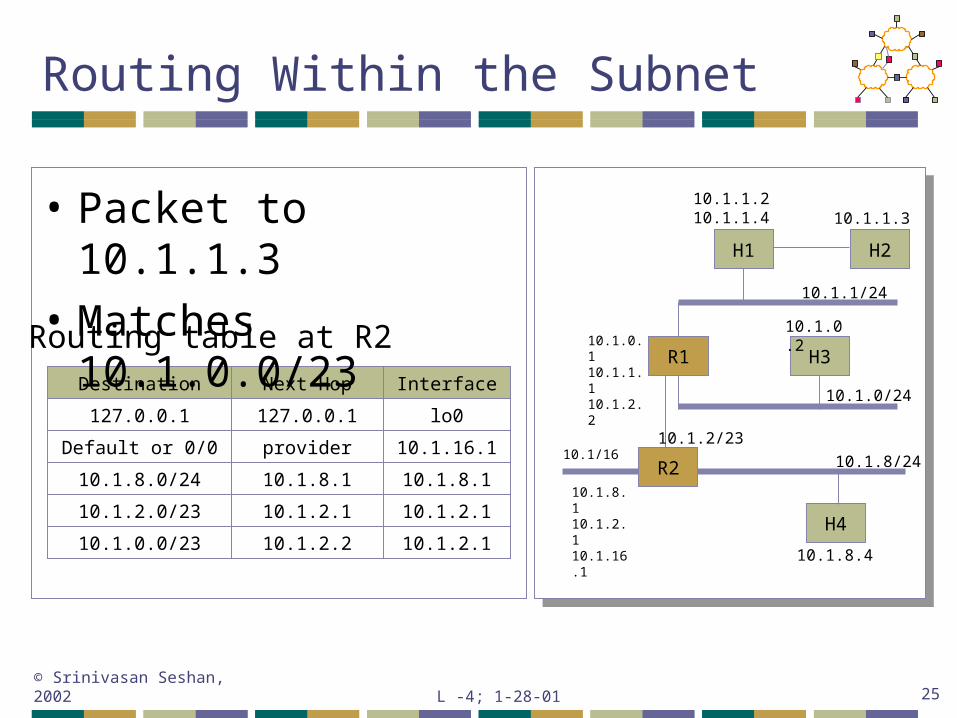
Routing Within the Subnet
Routing table at R2
H2
H3
H4
R1
10.1.1/24
10.1/16 10.1.8/24
10.1.0/24
10.1.1.3
10.1.2/23
R2
10.1.0.2
10.1.8.4
10.1.0.110.1.1.110.1.2.2
10.1.8.110.1.2.110.1.16.1
H1
Destination Next Hop Interface
127.0.0.1 127.0.0.1 lo0
Default or 0/0 provider 10.1.16.1
10.1.8.0/24 10.1.8.1 10.1.8.1
10.1.2.0/23 10.1.2.1 10.1.2.1
10.1.0.0/23 10.1.2.2 10.1.2.1
• Packet to 10.1.1.3
• Matches 10.1.0.0/23
10.1.1.210.1.1.4
L -4; 1-28-01© Srinivasan Seshan, 2002 26
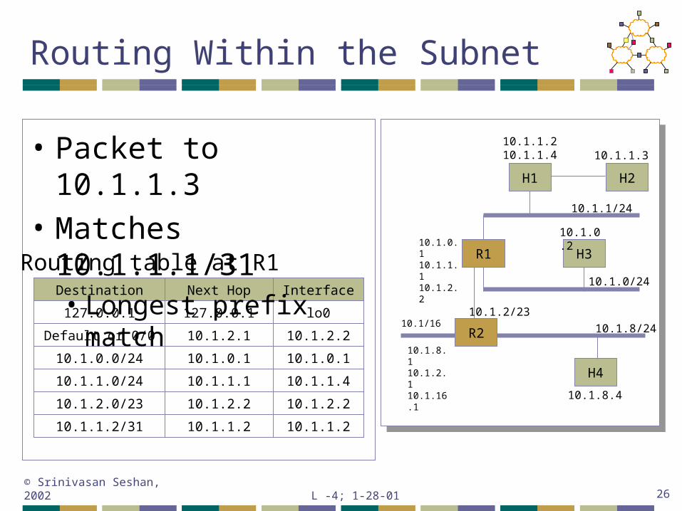
Routing Within the Subnet
H2
H3
H4
R1
10.1.1/24
10.1/16 10.1.8/24
10.1.0/24
10.1.1.3
10.1.2/23
R2
10.1.0.2
10.1.8.4
10.1.0.110.1.1.110.1.2.2
10.1.8.110.1.2.110.1.16.1
H1
Routing table at R1Destination Next Hop Interface
127.0.0.1 127.0.0.1 lo0
Default or 0/0 10.1.2.1 10.1.2.2
10.1.0.0/24 10.1.0.1 10.1.0.1
10.1.1.0/24 10.1.1.1 10.1.1.4
10.1.2.0/23 10.1.2.2 10.1.2.2
• Packet to 10.1.1.3
• Matches 10.1.1.1/31• Longest prefix match
10.1.1.2/31 10.1.1.2 10.1.1.2
10.1.1.210.1.1.4
L -4; 1-28-01© Srinivasan Seshan, 2002 27
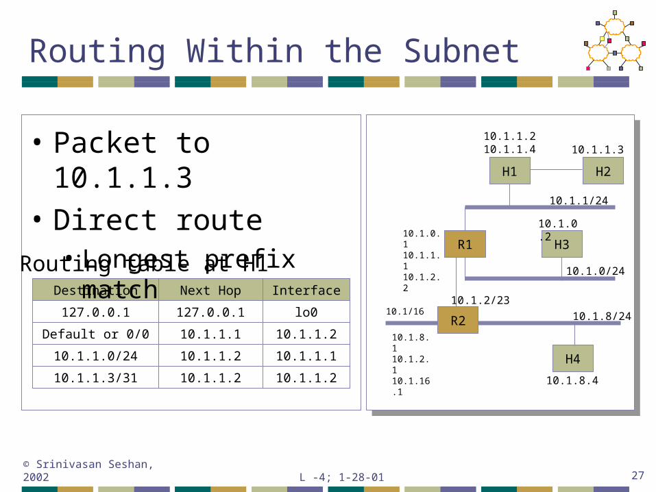
Routing Within the Subnet
H2
H3
H4
R1
10.1.1/24
10.1/16 10.1.8/24
10.1.0/24
10.1.1.3
10.1.2/23
R2
10.1.0.2
10.1.8.4
10.1.0.110.1.1.110.1.2.2
10.1.8.110.1.2.110.1.16.1
H1
Routing table at H1Destination Next Hop Interface
127.0.0.1 127.0.0.1 lo0
Default or 0/0 10.1.1.1 10.1.1.2
10.1.1.0/24 10.1.1.2 10.1.1.1
10.1.1.3/31 10.1.1.2 10.1.1.2
• Packet to 10.1.1.3
• Direct route• Longest prefix match
10.1.1.210.1.1.4
L -4; 1-28-01© Srinivasan Seshan, 2002 28
Global Addresses
• Advantages• Stateless – simple error recovery
• Disadvantages• Every switch knows about every destination
• Potentially large tables
• All packets to destination take same route
L -4; 1-28-01© Srinivasan Seshan, 2002 29
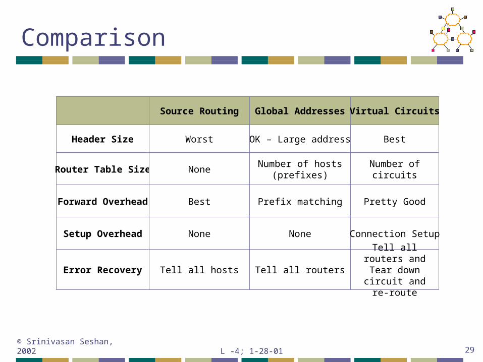
Comparison
Source Routing Global Addresses
Header Size Worst OK – Large address
Router Table Size NoneNumber of hosts
(prefixes)
Forward Overhead Best Prefix matching
Virtual Circuits
Best
Number of circuits
Pretty Good
Setup Overhead None None
Error Recovery Tell all hosts Tell all routers
Connection Setup
Tell all routers and Tear down circuit
and re-route
L -4; 1-28-01© Srinivasan Seshan, 2002 30
How do we set up Routing Tables?
• Graph theory to compute “shortest path”• Switches = nodes• Links = edges• Delay, hops = cost
• Need to adapt to changes in topology
L -4; 1-28-01© Srinivasan Seshan, 2002 31
Outline
• Alternative methods for packet forwarding
• IP packet routing
• Variable prefix match
• Packet classification
L -4; 1-28-01© Srinivasan Seshan, 2002 32
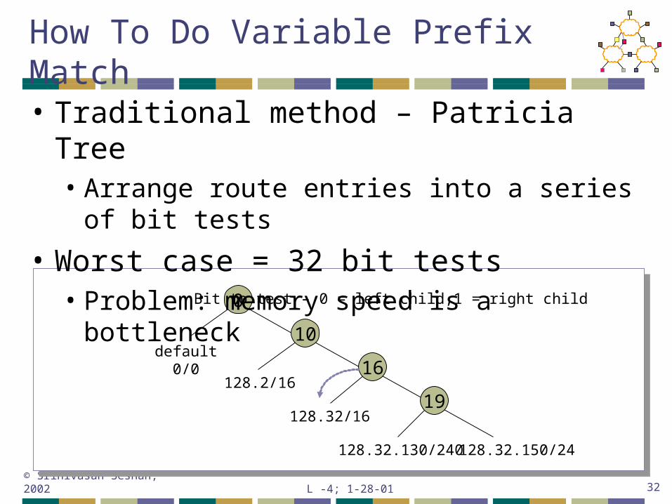
How To Do Variable Prefix Match
128.2/16
10
16
19128.32/16
128.32.130/240 128.32.150/24
default0/0
0
• Traditional method – Patricia Tree• Arrange route entries into a series of bit tests
• Worst case = 32 bit tests• Problem: memory speed is a bottleneck
Bit to test – 0 = left child,1 = right child
L -4; 1-28-01© Srinivasan Seshan, 2002 33
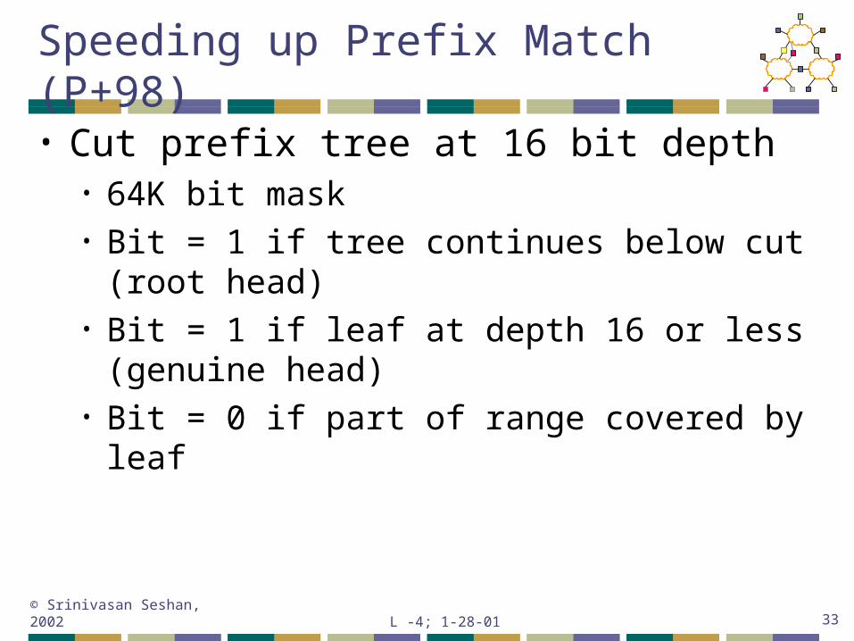
Speeding up Prefix Match (P+98)
• Cut prefix tree at 16 bit depth • 64K bit mask• Bit = 1 if tree continues below cut (root head)• Bit = 1 if leaf at depth 16 or less (genuine head)• Bit = 0 if part of range covered by leaf
L -4; 1-28-01© Srinivasan Seshan, 2002 34
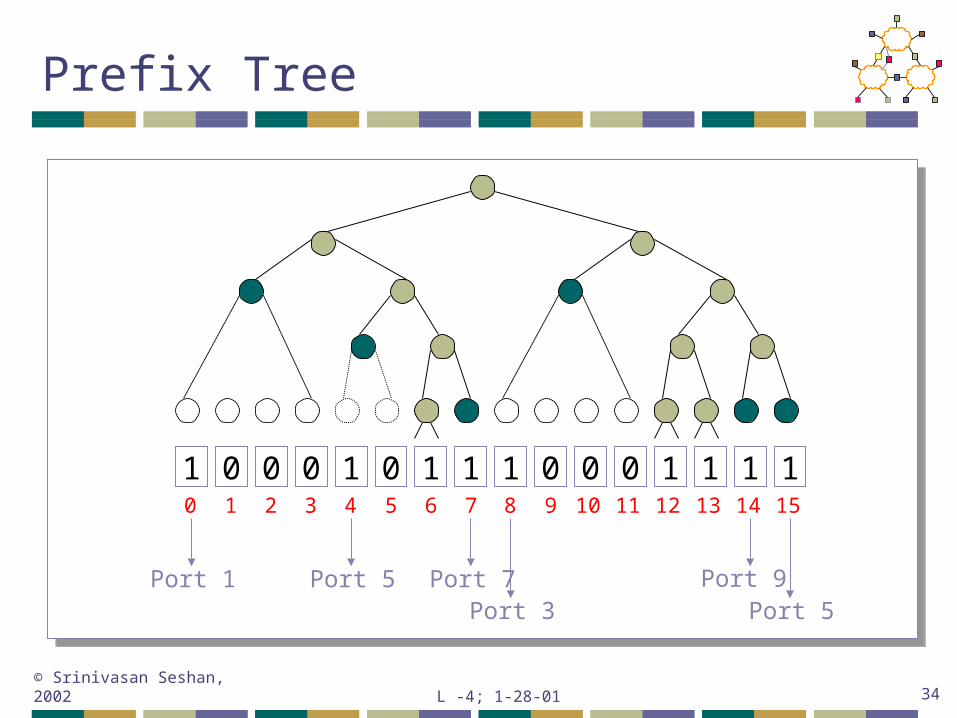
Prefix Tree
10
0 0 0 1 0 1 1 1 0 0 0 1 1 1 11 2 3 4 5 6 7 8 9 10 11 12 13 14 15
Port 1 Port 5 Port 7Port 3
Port 9Port 5
L -4; 1-28-01© Srinivasan Seshan, 2002 35
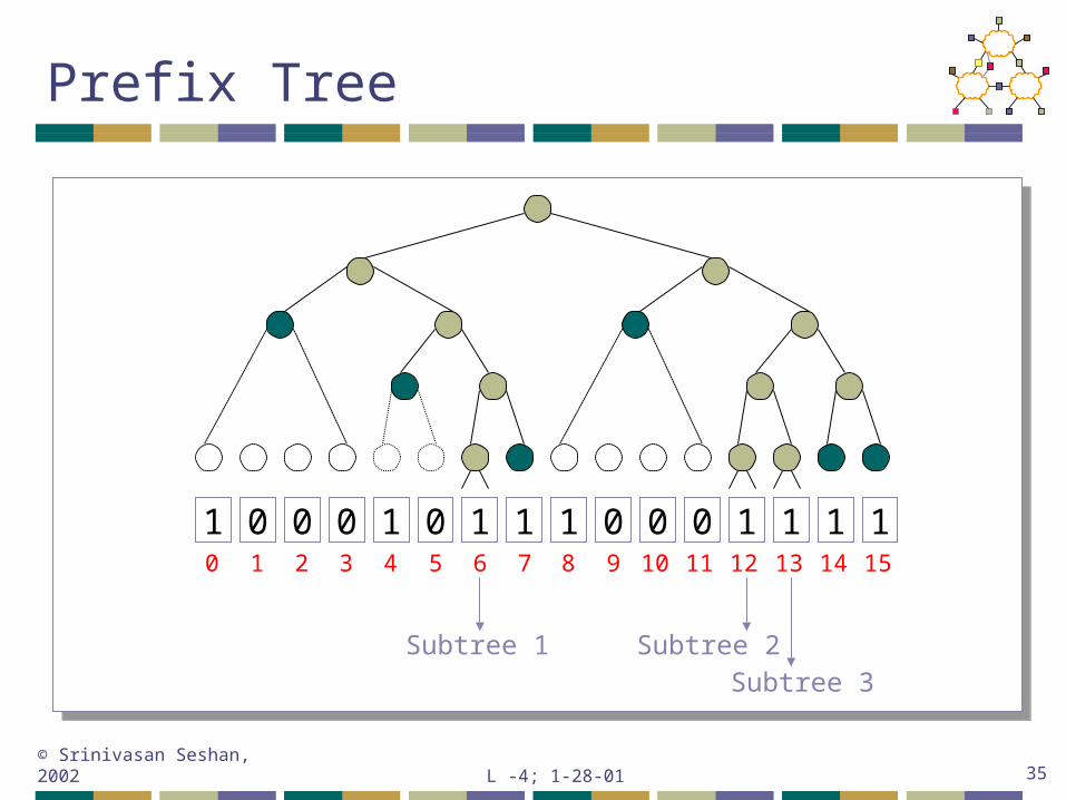
Prefix Tree
10
0 0 0 1 0 1 1 1 0 0 0 1 1 1 11 2 3 4 5 6 7 8 9 10 11 12 13 14 15
Subtree 1 Subtree 2
Subtree 3
L -4; 1-28-01© Srinivasan Seshan, 2002 36
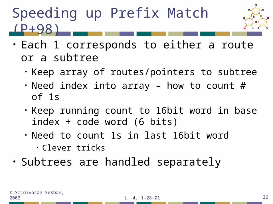
Speeding up Prefix Match (P+98)
• Each 1 corresponds to either a route or a subtree• Keep array of routes/pointers to subtree• Need index into array – how to count # of 1s• Keep running count to 16bit word in base index
+ code word (6 bits)• Need to count 1s in last 16bit word
• Clever tricks
• Subtrees are handled separately

L -4; 1-28-01© Srinivasan Seshan, 2002 37
Speeding up Prefix Match (P+98)
• Scaling issues• How would it handle IPv6
• Other possiblities• Why were the cuts done at 16/24/32 bits?• Improve data structure by shuffling bits
L -4; 1-28-01© Srinivasan Seshan, 2002 38
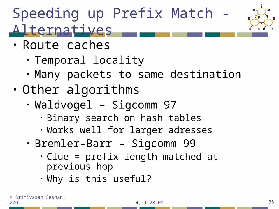
Speeding up Prefix Match - Alternatives
• Route caches• Temporal locality• Many packets to same destination
• Other algorithms • Waldvogel – Sigcomm 97
• Binary search on hash tables• Works well for larger adresses
• Bremler-Barr – Sigcomm 99• Clue = prefix length matched at previous hop• Why is this useful?
L -4; 1-28-01© Srinivasan Seshan, 2002 39
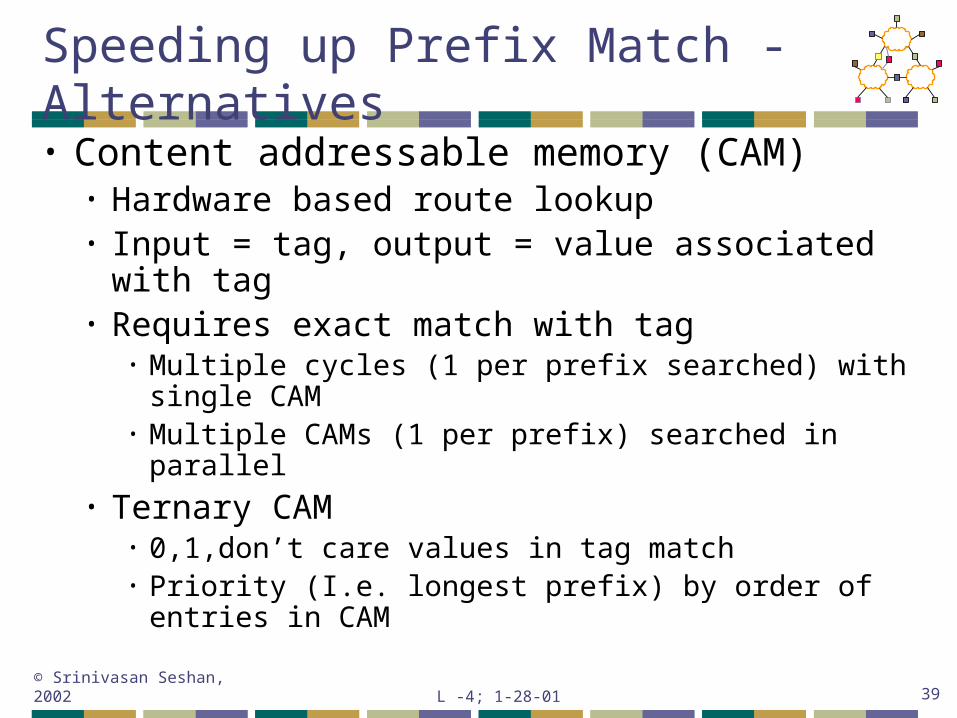
Speeding up Prefix Match - Alternatives
• Content addressable memory (CAM)• Hardware based route lookup• Input = tag, output = value associated with tag• Requires exact match with tag
• Multiple cycles (1 per prefix searched) with single CAM
• Multiple CAMs (1 per prefix) searched in parallel• Ternary CAM
• 0,1,don’t care values in tag match• Priority (I.e. longest prefix) by order of entries in
CAM
L -4; 1-28-01© Srinivasan Seshan, 2002 40
Outline
• Alternative methods for packet forwarding
• IP packet routing
• Variable prefix match
• Packet classification
L -4; 1-28-01© Srinivasan Seshan, 2002 41
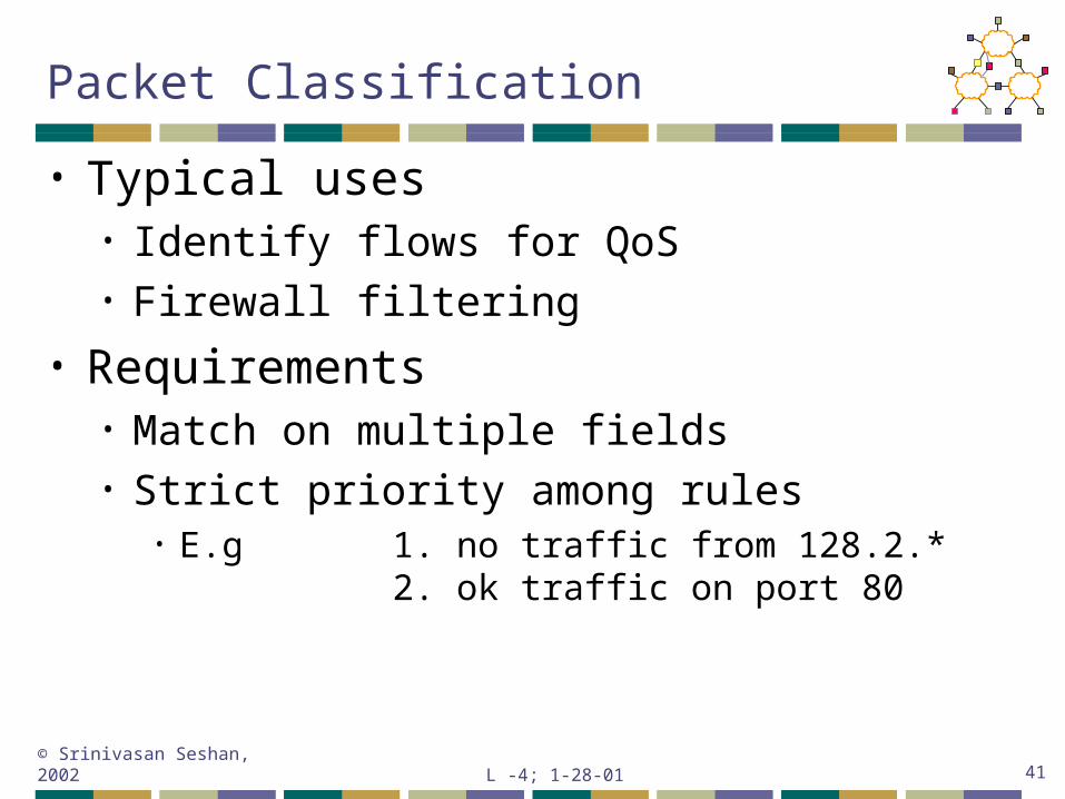
Packet Classification
• Typical uses• Identify flows for QoS• Firewall filtering
• Requirements• Match on multiple fields• Strict priority among rules
• E.g 1. no traffic from 128.2.*2. ok traffic on port 80
L -4; 1-28-01© Srinivasan Seshan, 2002 42
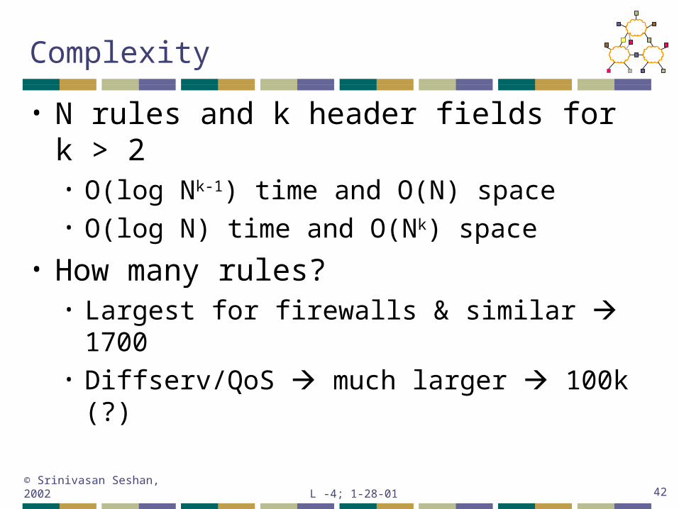
Complexity
• N rules and k header fields for k > 2• O(log Nk-1) time and O(N) space• O(log N) time and O(Nk) space
• How many rules?• Largest for firewalls & similar 1700• Diffserv/QoS much larger 100k (?)
L -4; 1-28-01© Srinivasan Seshan, 2002 43
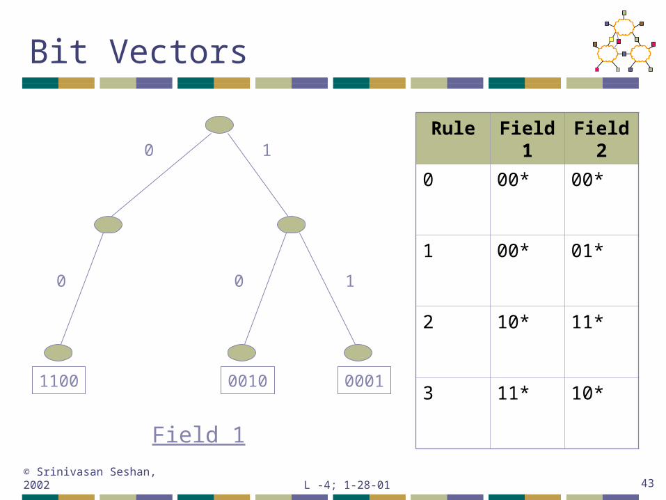
Bit Vectors
0 1
0 0 1
000100101100
Rule Field1 Field2
0 00* 00*
1 00* 01*
2 10* 11*
3 11* 10*
Field 1
L -4; 1-28-01© Srinivasan Seshan, 2002 44
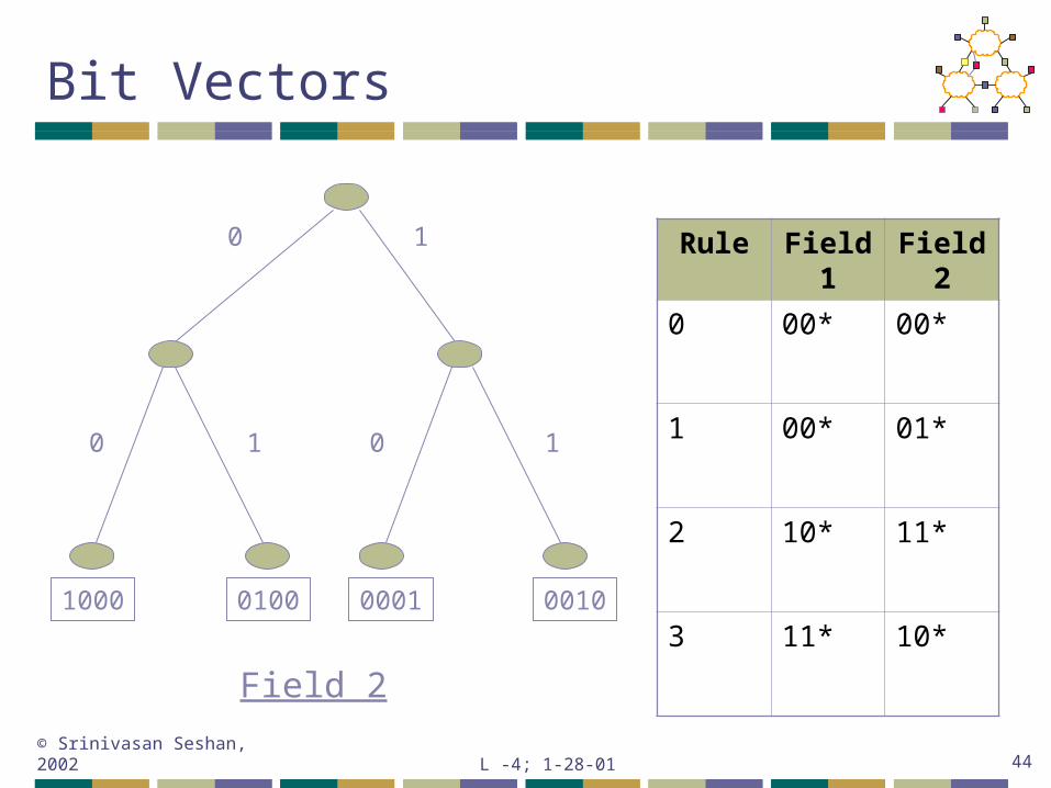
Bit Vectors
0 1
0 0 1
001000011000
Rule Field1 Field2
0 00* 00*
1 00* 01*
2 10* 11*
3 11* 10*0100
1
Field 2
L -4; 1-28-01© Srinivasan Seshan, 2002 45
Observations [GM99]
• Common rule sets have important/useful characteristics• Packets rarely match more than a few rules
(rule intersection)• E.g., max of 4 rules seen on common databases up
to 1700 rules
• Special cases for k = 2 source and destination
• O(log N) time and O(N) space solutions exist
L -4; 1-28-01© Srinivasan Seshan, 2002 46
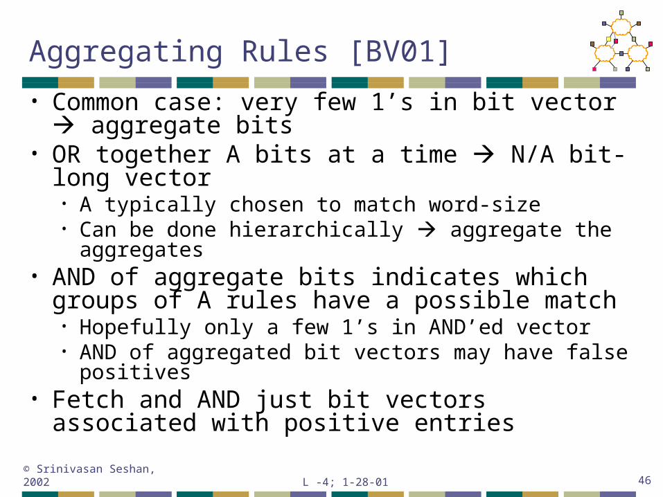
Aggregating Rules [BV01]
• Common case: very few 1’s in bit vector aggregate bits
• OR together A bits at a time N/A bit-long vector• A typically chosen to match word-size• Can be done hierarchically aggregate the
aggregates• AND of aggregate bits indicates which groups of
A rules have a possible match• Hopefully only a few 1’s in AND’ed vector• AND of aggregated bit vectors may have false positives
• Fetch and AND just bit vectors associated with positive entries
L -4; 1-28-01© Srinivasan Seshan, 2002 47
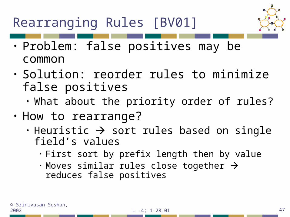
Rearranging Rules [BV01]
• Problem: false positives may be common• Solution: reorder rules to minimize false
positives• What about the priority order of rules?
• How to rearrange?• Heuristic sort rules based on single field’s
values• First sort by prefix length then by value• Moves similar rules close together reduces false
positives
L -4; 1-28-01© Srinivasan Seshan, 2002 48
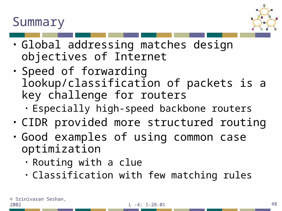
Summary
• Global addressing matches design objectives of Internet
• Speed of forwarding lookup/classification of packets is a key challenge for routers• Especially high-speed backbone routers
• CIDR provided more structured routing• Good examples of using common case
optimization• Routing with a clue• Classification with few matching rules
L -4; 1-28-01© Srinivasan Seshan, 2002 49
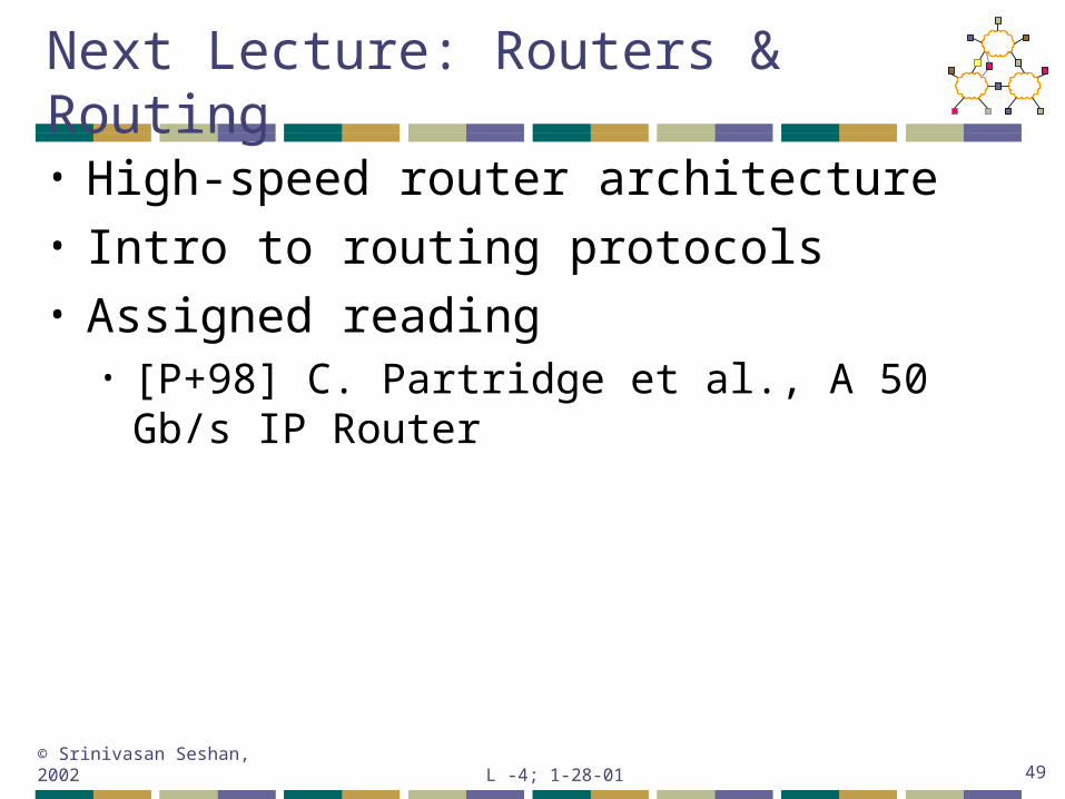
Next Lecture: Routers & Routing
• High-speed router architecture• Intro to routing protocols• Assigned reading
• [P+98] C. Partridge et al., A 50 Gb/s IP Router


![15-744: Computer Networking L-14 Naming. L -14; 10-24-02© Srinivasan Seshan, 20022 Naming DNS Assigned reading [JSBM01] DNS Performance and the Effectiveness](https://img.pdfslide.us/doc/110x75/56649f475503460f94c68d99/15-744-computer-networking-l-14-naming-l-14-10-24-02-srinivasan-seshan.jpg)


![15-744: Computer Networking L-23 Security. L -23; 4-17-02© Srinivasan Seshan, 20022 Security Denial of service IPSec Firewalls Assigned reading [SWKA00]](https://img.pdfslide.us/doc/110x75/56649d825503460f94a6702a/15-744-computer-networking-l-23-security-l-23-4-17-02-srinivasan-seshan.jpg)


![15-744: Computer Networking L-17 Security. L -17; 11-6-02© Srinivasan Seshan, 20022 Security Denial of service IPSec Firewalls Assigned reading [SWKA00]](https://img.pdfslide.us/doc/110x75/5a4d1acf7f8b9ab059970c46/15-744-computer-networking-l-17-security-l-17-11-6-02-srinivasan.jpg)


![15-744: Computer Networking L-22: P2P. L -22; 4-15-02© Srinivasan Seshan, 20022 P2P Peer-to-peer networks Assigned reading [Cla00] Freenet: A Distributed](https://img.pdfslide.us/doc/110x75/5697c02b1a28abf838cd85b2/15-744-computer-networking-l-22-p2p-l-22-4-15-02-srinivasan-seshan.jpg)