15

1

Grossberg Network

15

2

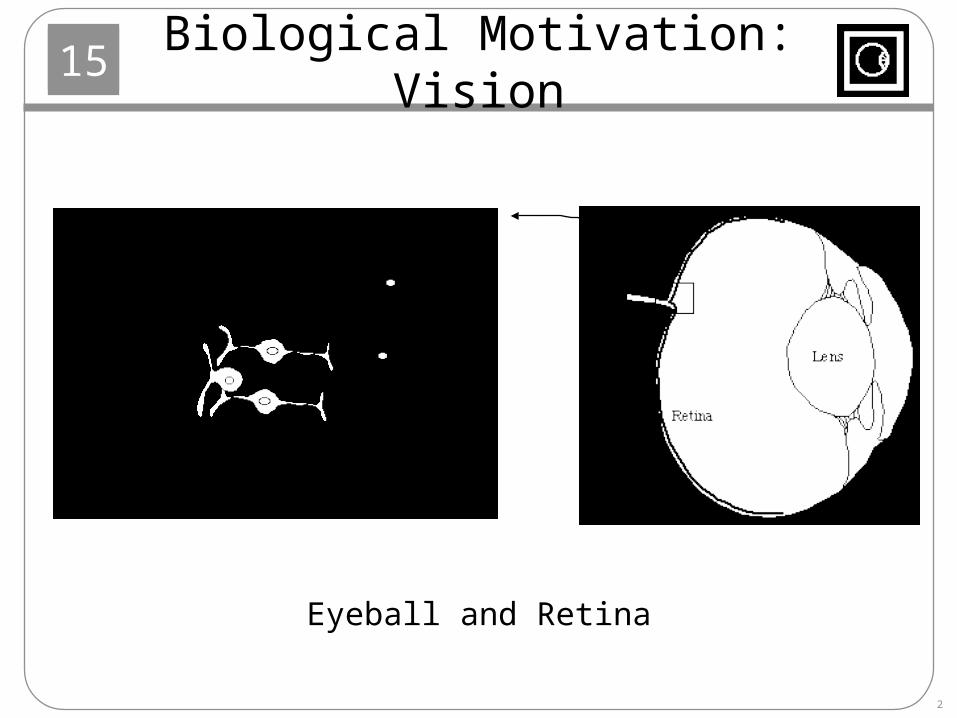
Biological Motivation: Vision

Eyeball and Retina

15

3

Layers of Retina

The retina is a part of the brain that covers the back innerwall of the eye and consists of three layers of neurons:

Outer Layer:Photoreceptors - convert light into electrical signals

Rods - allow us to see in dim lightCones - fine detail and color

Middle LayerBipolar Cells - link photoreceptors to third layerHorizontal Cells - link receptors with bipolar cellsAmacrine Cells - link bipolar cells with ganglion cells

Final LayerGanglion Cells - link retina to brain through optic nerve

15

4

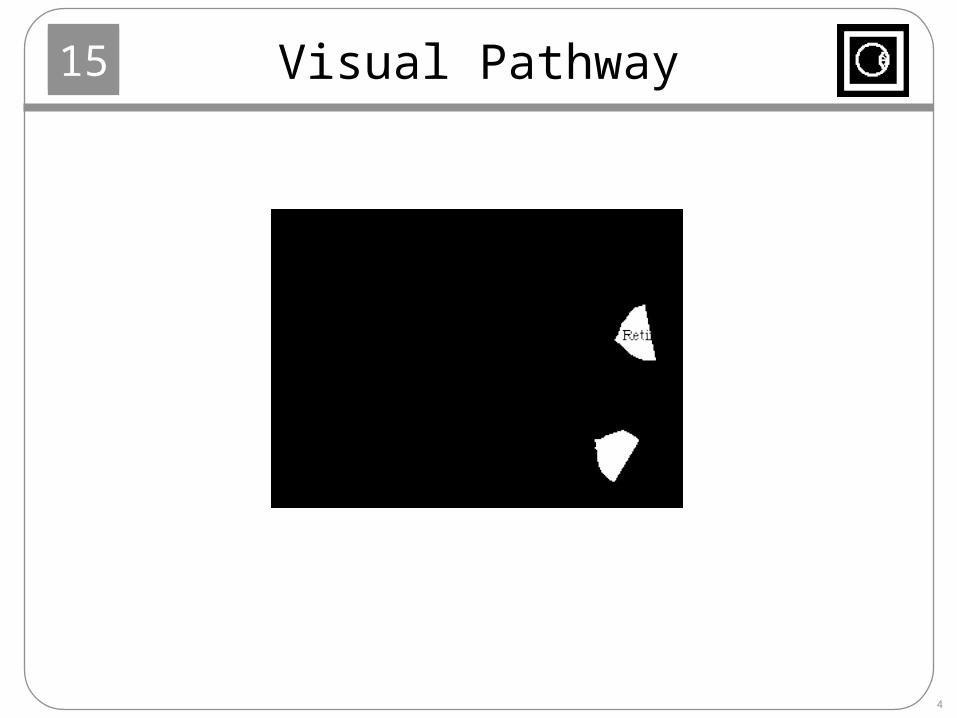
Visual Pathway

15

5

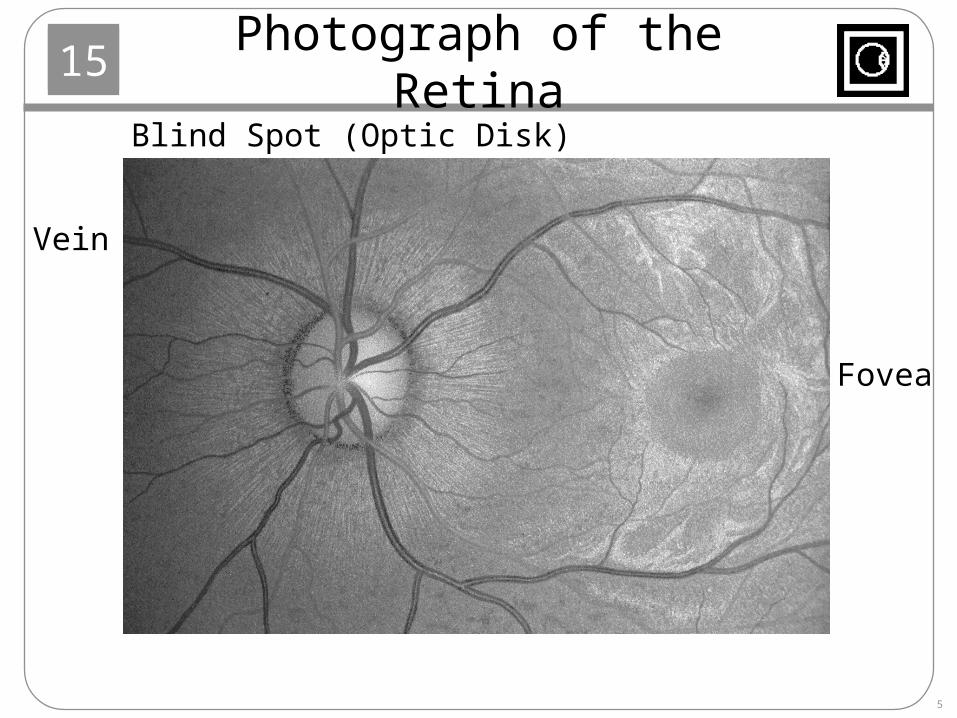
Photograph of the Retina

Blind Spot (Optic Disk)

Vein

Fovea

15

6

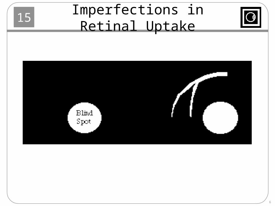
Imperfections in Retinal Uptake

15

7

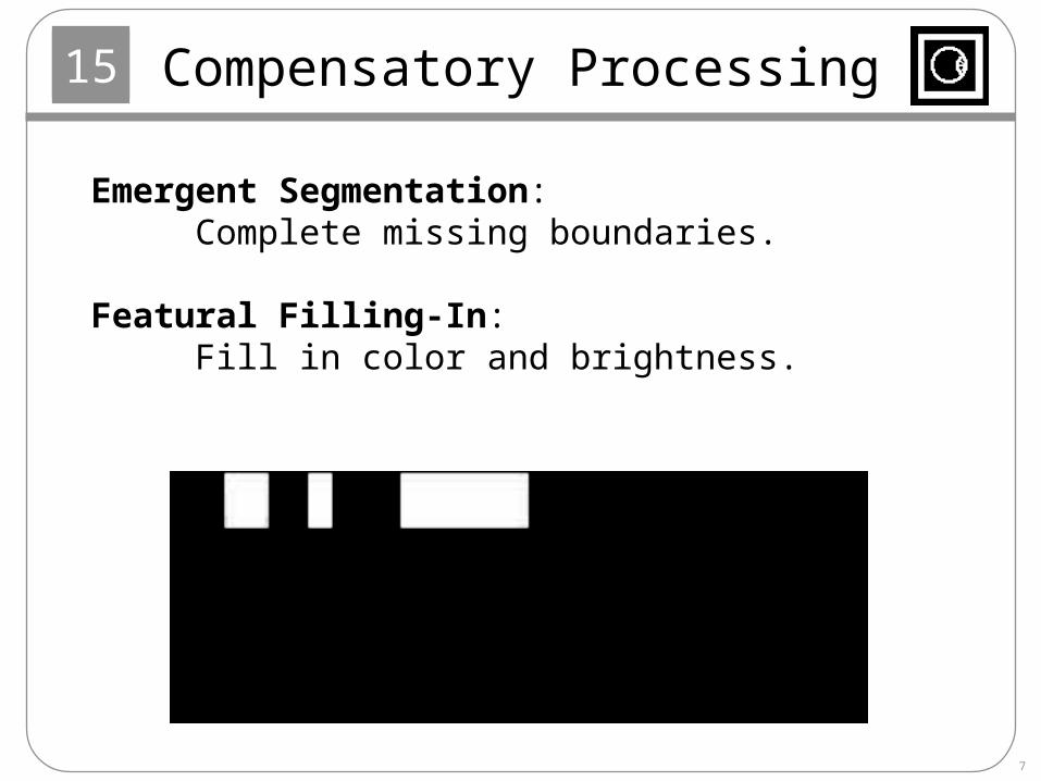
Compensatory Processing

Emergent Segmentation:Complete missing boundaries.

Featural Filling-In:Fill in color and brightness.

15

8

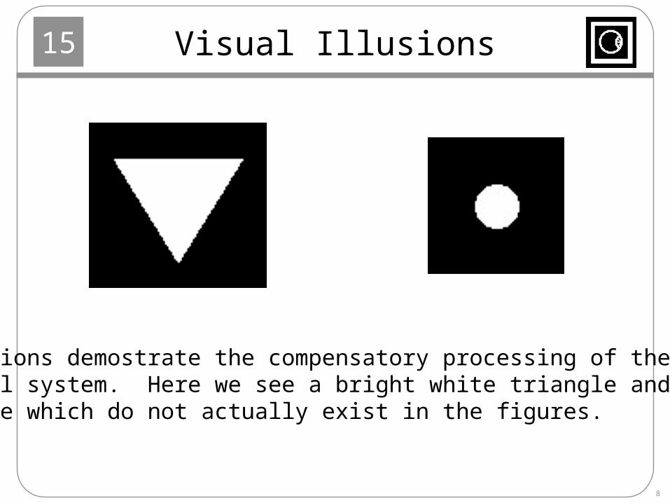
Visual Illusions

Illusions demostrate the compensatory processing of thevisual system. Here we see a bright white triangle and a circle which do not actually exist in the figures.

15

9

Vision Normalization

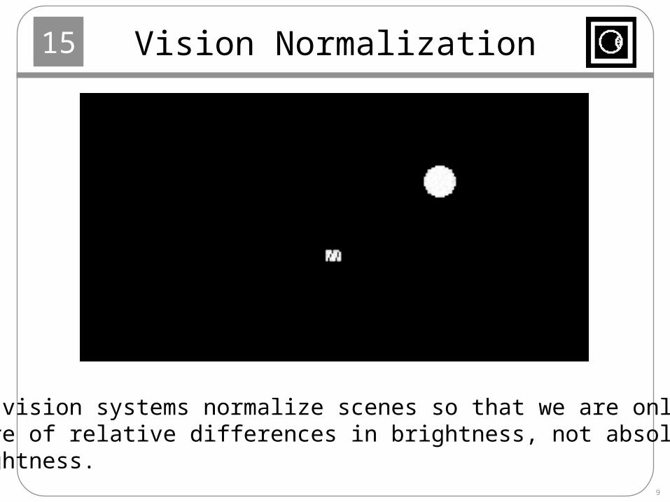
The vision systems normalize scenes so that we are onlyaware of relative differences in brightness, not absolutebrightness.

15

10

Brightness Contrast

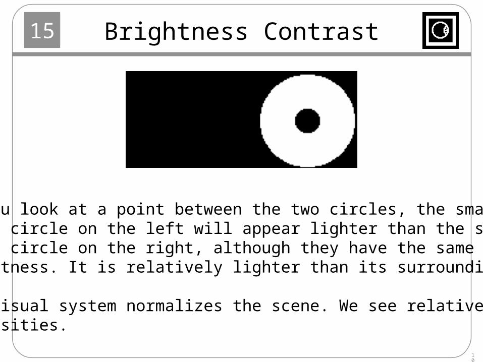
If you look at a point between the two circles, the smallinner circle on the left will appear lighter than the smallinner circle on the right, although they have the samebrightness. It is relatively lighter than its surroundings.

The visual system normalizes the scene. We see relativeintensities.

15

11

Leaky Integrator

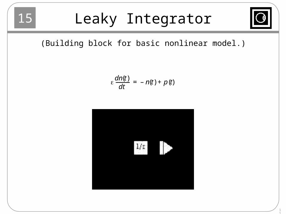
dn t( )dt

------------ n t( )– p t( )+=

(Building block for basic nonlinear model.)

15

12

Leaky Integrator Response

0 1 2 3 4 50

0.25

0.5

0.75

1

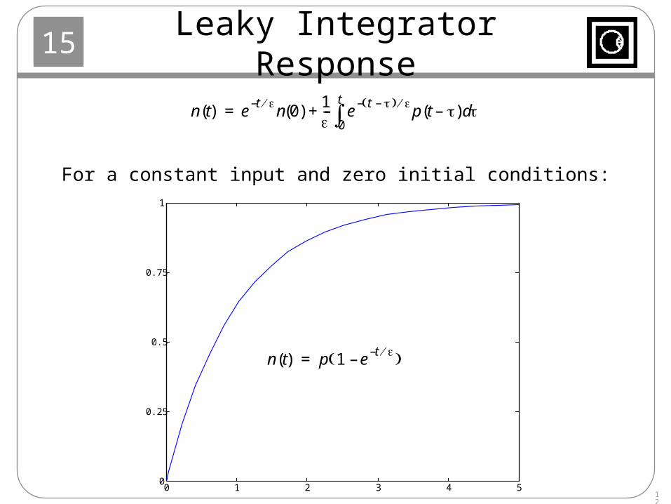
n t( ) et –n 0( )

1--- e

t – –p t –( ) d

0

t

+=

n t( ) p 1 et –

– =

For a constant input and zero initial conditions:

15

13

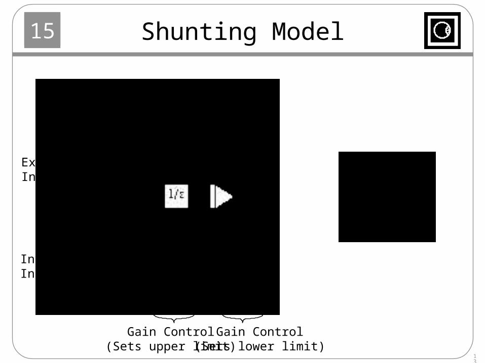
Shunting Model

Gain Control(Sets lower limit)

Gain Control(Sets upper limit)

ExcitatoryInput

InhibitoryInput

15

14

Shunting Model Response

0 1 2 3 4 50

0.25

0.5

0.75

1

0 1 2 3 4 50

0.25

0.5

0.75

1

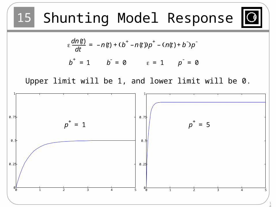
dn t( )dt

------------ n t( )– b+n t( )– p+

n t( ) b-

+ p-–+=

b+

1= b-

0= 1= p-

0=

p+

1= p+

5=

Upper limit will be 1, and lower limit will be 0.

15

15

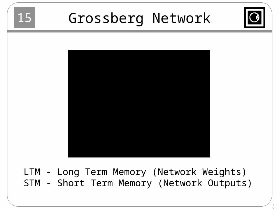
Grossberg Network

LTM - Long Term Memory (Network Weights)STM - Short Term Memory (Network Outputs)

15

16

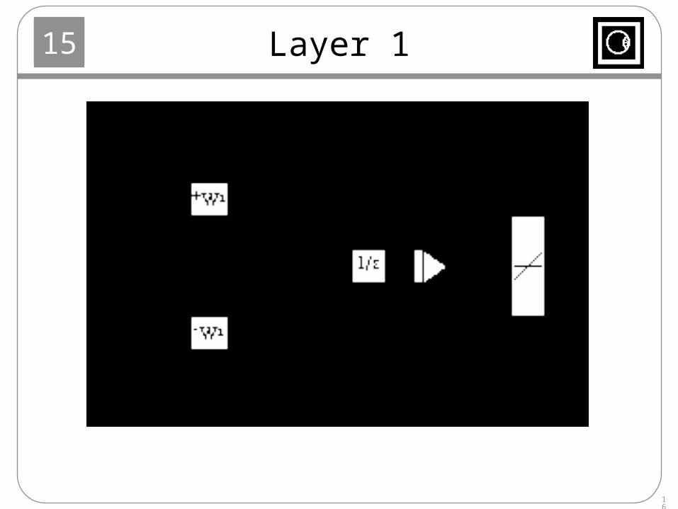
Layer 1

15

17

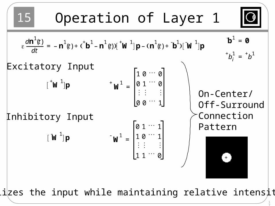
Operation of Layer 1

dn1

t( )dt

--------------- n1t( )– b

+ 1n

1t( )– W

+ 1 p n

1t( ) b

- 1+ W

- 1 p–+=

Excitatory Input

W+ 1

1 0 0

0 1 0

0 0 1

=W+ 1

p

Inhibitory Input W

- 1

0 1 1

1 0 1

1 1 0

=W- 1

p

On-Center/Off-SurroundConnectionPattern

Normalizes the input while maintaining relative intensities.

b- 1 0=

b+ 1i b

+ 1=

15

18

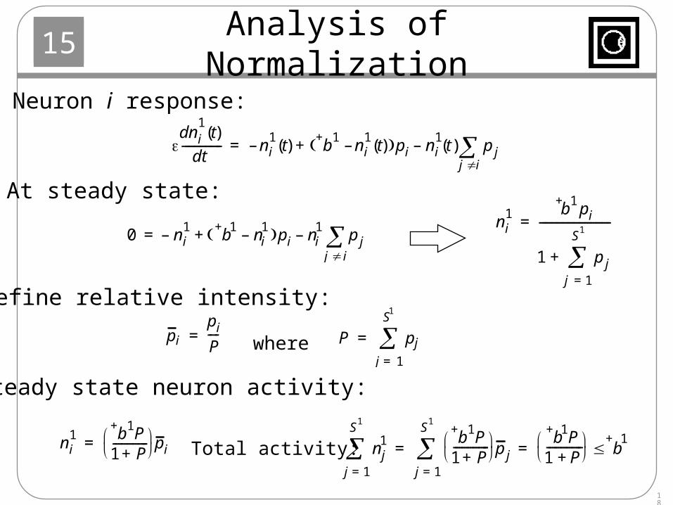
Analysis of Normalization

dni

1t( )

dt-------------- ni

1t( )– b

+ 1ni

1t( )– pi ni

1t( ) p jj i–+=

Neuron i response:

At steady state:

0 ni1

– b+ 1

ni1

– pi ni1

p jj i–+=

ni1 b

+ 1pi

1 p jj 1=

S1

+

-------------------------=

pipiP----= P pj

j 1=

S1

=

Define relative intensity:

Steady state neuron activity:

ni1 b

+ 1P

1 P+-------------

pi= nj1

j 1=

S1

b+ 1P1 P+-------------

p jj 1=

S1

b+ 1P1 P+-------------

b+ 1

= =

where

Total activity:

15

19

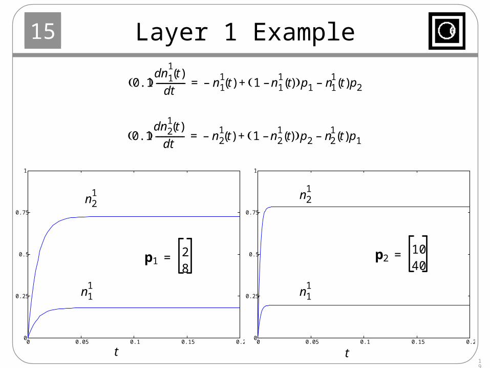
Layer 1 Example

0 0.05 0.1 0.15 0.20

0.25

0.5

0.75

1

0 0.05 0.1 0.15 0.20

0.25

0.5

0.75

1

0.1 dn1

1t( )

dt-------------- n1

1t( )– 1 n1

1t( )– p1 n1

1t( )p2–+=

0.1 dn2

1t( )

dt-------------- n2

1t( )– 1 n2

1t( )– p2 n2

1t( )p1–+=

t

n11

n21

p128

=

t

n11

n21

p21040

=

15

20

Characteristics of Layer 1

• The network is sensitive to relative intensities of the input pattern, rather than absolute intensities.

• The output of Layer 1 is a normalized version of the input pattern.

• The on-center/off-surround connection pattern and the nonlinear gain control of the shunting model produce the normalization effect.

• The operation of Layer 1 explains the brightness constancy and brightness contrast characteristics of the human visual system.

15

21

Layer 2

15

22

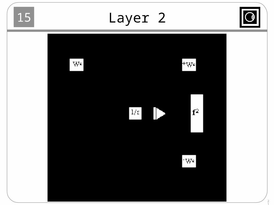
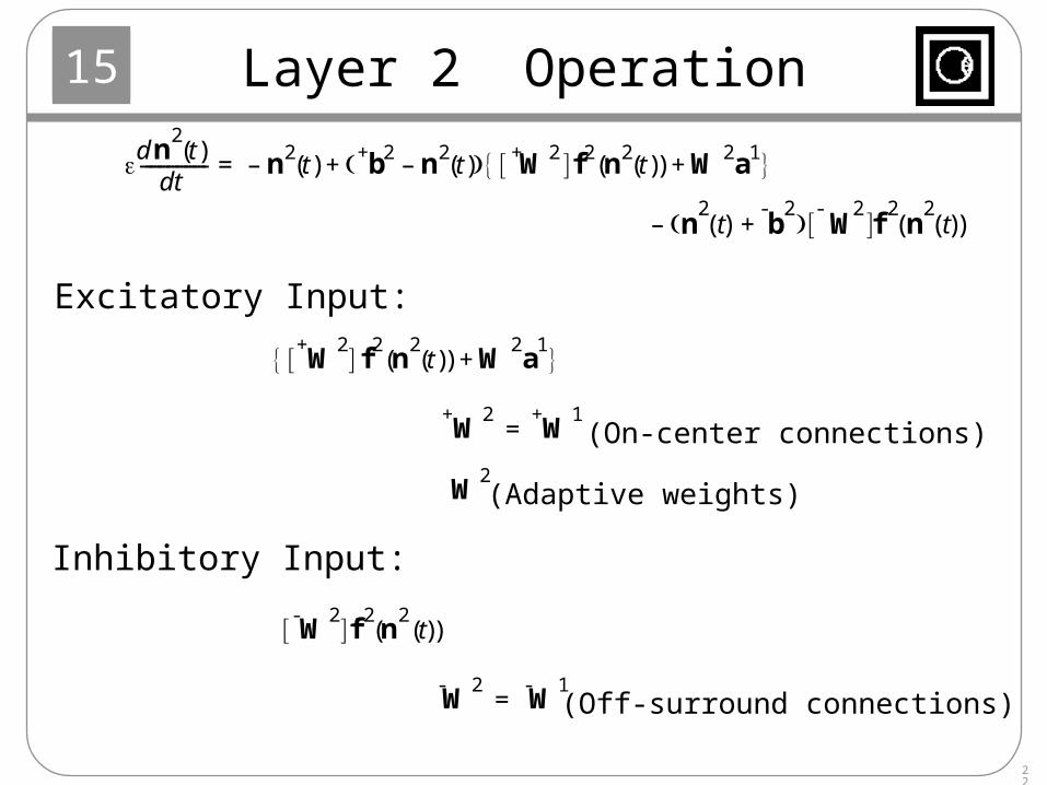
Layer 2 Operation

dn2t( )

dt--------------- n2

t( )– b+ 2 n2t( )– W+ 2 f2 n2

t( )( ) W2a1+ +=

n2t( ) b

- 2+ W

- 2 f

2n

2t( )( )–

W+ 2 f

2n

2t( )( ) W

2a

1+

Excitatory Input:

W+ 2

W+ 1

= (On-center connections)

Inhibitory Input:

W2

(Adaptive weights)

W- 2 f

2n

2t( )( )

W- 2

W- 1

= (Off-surround connections)

15

23

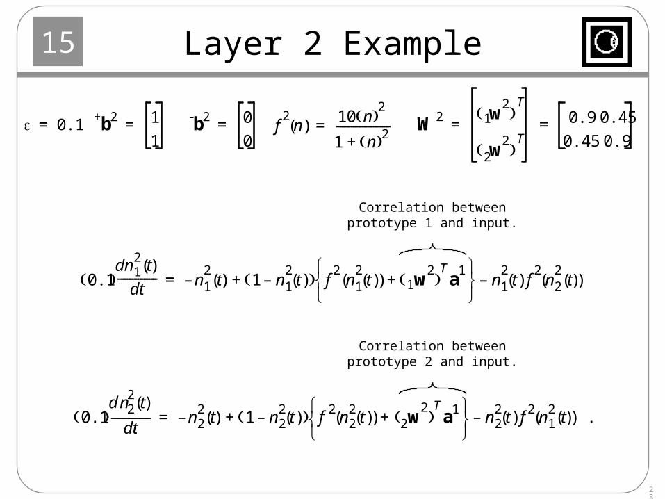
Layer 2 Example

0.1= b+ 2 1

1= b- 2 0

0= W2 w

21

T

w2

2 T

0.9 0.45

0.45 0.9= =f

2n( )

10 n 2

1 n 2+-------------------=

0.1 dn1

2t( )

dt-------------- n1

2t( )– 1 n1

2t( )– f

2n1

2t( )( ) w

21

Ta

1+

n12t( ) f

2n2

2t( )( )–+=

0.1 d n2

2t( )

dt-------------- n2

2t( )– 1 n2

2t( )– f 2

n22t( )( ) w

22

Ta1

+

n22t( ) f

2n1

2t( )( ) .–+=

Correlation betweenprototype 1 and input.

Correlation betweenprototype 2 and input.

15

24

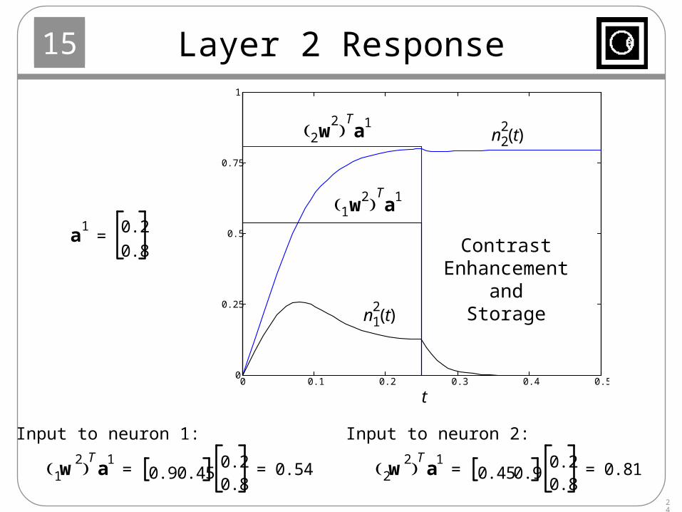
Layer 2 Response

a1 0.2

0.8=

w2

1 Ta

10.9 0.45

0.20.8

0.54= =

0 0.1 0.2 0.3 0.4 0.50

0.25

0.5

0.75

1

t

w21

Ta1

w2

2 Ta1

n12t( )

n22t( )

w2

2 Ta

10.45 0.9

0.20.8

0.81= =

ContrastEnhancement

andStorage

Input to neuron 1: Input to neuron 2:

15

25

Characteristics of Layer 2

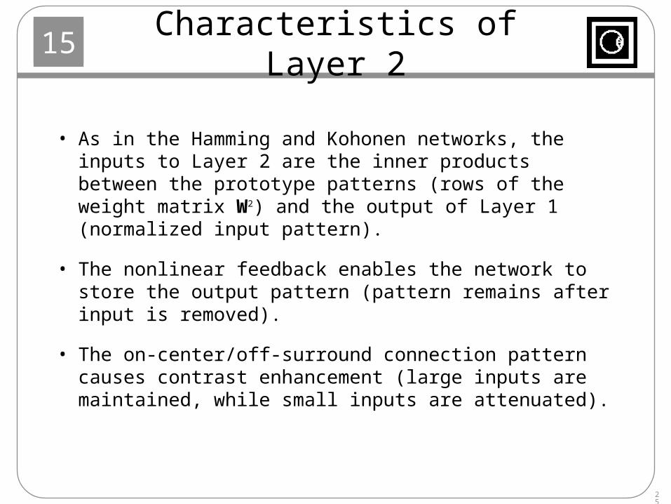
• As in the Hamming and Kohonen networks, the inputs to Layer 2 are the inner products between the prototype patterns (rows of the weight matrix W2) and the output of Layer 1 (normalized input pattern).

• The nonlinear feedback enables the network to store the output pattern (pattern remains after input is removed).

• The on-center/off-surround connection pattern causes contrast enhancement (large inputs are maintained, while small inputs are attenuated).

15

26

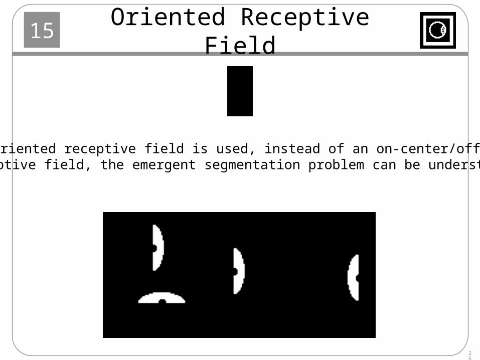
Oriented Receptive Field

When an oriented receptive field is used, instead of an on-center/off-surroundreceptive field, the emergent segmentation problem can be understood.

15

27

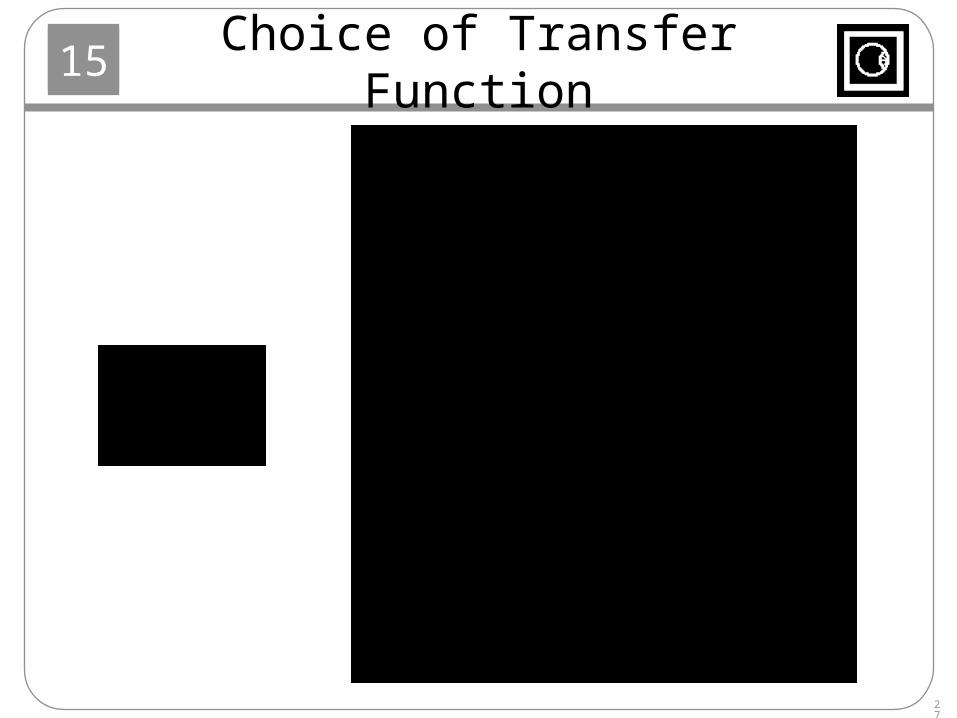
Choice of Transfer Function

15

28

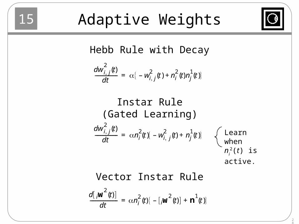
Adaptive Weights

dw i j2t( )

dt------------------ wi j

2t( )– ni

2t( )nj

1t( )+ =

dw i j2t( )

dt------------------ ni

2t( ) wi j

2t( )– nj

1t( )+ =

d w2

i t( ) dt

---------------------- ni2t( ) w

2i t( ) – n

1t( )+ =

Hebb Rule with Decay

Instar Rule(Gated Learning)

Vector Instar Rule

Learn whenni2(t) is active.

15

29

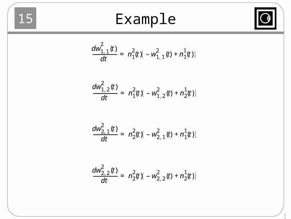
Example

dw1 12t( )

dt-------------------- n1

2t( ) w1 1

2t( )– n1

1t( )+ =

dw1 22t( )

dt-------------------- n1

2t( ) w1 2

2t( )– n2

1t( )+ =

dw2 12t( )

dt-------------------- n2

2t( ) w2 1

2t( )– n1

1t( )+ =

dw2 22t( )

dt-------------------- n2

2t( ) w2 2

2t( )– n2

1t( )+ =

15

30

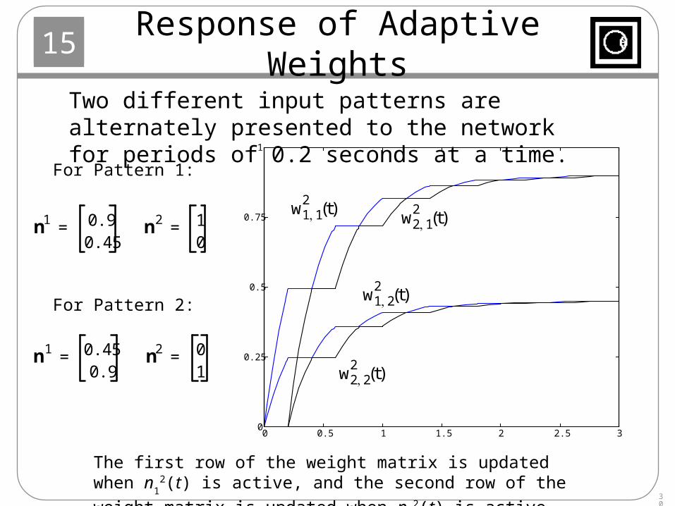
Response of Adaptive Weights

n1 0.90.45

= n2 10

=

n1 0.450.9

= n2 01

=

For Pattern 1:

For Pattern 2:

0 0.5 1 1.5 2 2.5 30

0.25

0.5

0.75

1

w1 12

t( )

w1 22

t( )

w2 12

t( )

w2 22

t( )

The first row of the weight matrix is updated when n1

2(t) is active, and

the second row of the weight matrix is updated when n2

2(t) is active.

Two different input patterns are alternately presented to the network for periods of 0.2 seconds at a time.

15

31

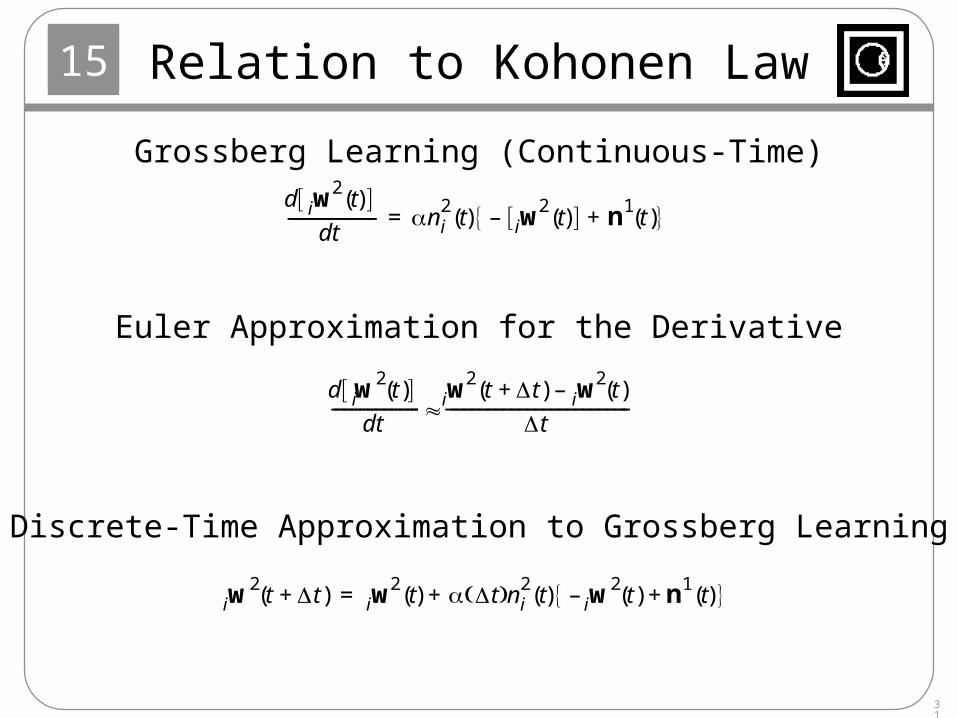
Relation to Kohonen Law

d w2i t( ) dt

---------------------- ni2t( ) w2

i t( ) – n1t( )+ =

d w2i t( ) dt

----------------------w2i t t+( ) w2

i t( )–

t----------------------------------------------

w2i t t+( ) w2

i t( ) t ni2t( ) w2

i t( )– n1t( )+ +=

Grossberg Learning (Continuous-Time)

Euler Approximation for the Derivative

Discrete-Time Approximation to Grossberg Learning

15

32

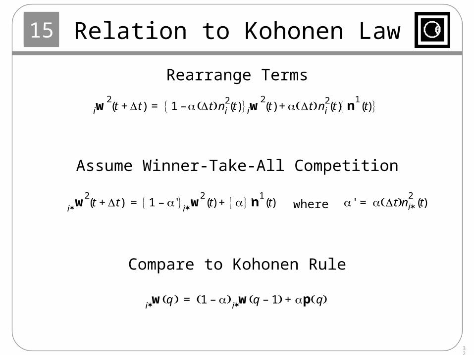
Relation to Kohonen Law

w2

i t t+( ) 1 '– w2

i t( ) 'n1t( )+= ' t ni

2t( )=

w2

i t t+( ) 1 t ni2t( )– w

2i t( ) t ni

2t( ) n

1t( ) +=

Rearrange Terms

Assume Winner-Take-All Competition

where

Compare to Kohonen Rule

wi q 1 – w

i q 1– p q +=