15-1 Copyright © 2013 Pearson Education, Inc. Publishing as Prentice Hall Forecasting Chapter 15

15-1Copyright © 2013 Pearson Education, Inc. Publishing as Prentice Hall

Forecasting

Chapter 15


■Forecasting Components

■Time Series Methods

■Forecast Accuracy

■Time Series Forecasting Using Excel

■Time Series Forecasting Using QM for

Windows

■Regression Methods

Chapter Topics


■ A variety of forecasting methods are available for use depending on the time frame of the forecast and the existence of patterns.

■ Time Frames: Short-range (one to two months) Medium-range (two months to one or two

years) Long-range (more than one or two years)

■ Patterns: Trend Random variations Cycles Seasonal pattern

Forecasting Components


Trend - A long-term movement of the item being forecast.

Random variations - movements that are not predictable and follow no pattern.

Cycle - A movement, up or down, that repeats itself over a lengthy time span.

Seasonal pattern - Oscillating movement in demand that occurs periodically in the short run.

Forecasting ComponentsPatterns (1 of 2)


Figure 15.1 (a) Trend; (b) Cycle; (c) Seasonal; (d) Trend with Season

Forecasting ComponentsPatterns (2 of 2)


Forecasting ComponentsForecasting Methods

1. Times Series - Statistical techniques that use historical data to predict future behavior.

2. Regression Methods - Regression (or causal ) methods that attempt to develop a mathematical relationship between the item being forecast and factors that cause it to behave the way it does.

3. Qualitative Methods - Methods using judgment, expertise and opinion to make forecasts.


Forecasting ComponentsQualitative Methods

“Jury of executive opinion,” a qualitative technique, is the most common type of forecast for long-term strategic planning. Performed by individuals or groups within an

organization, sometimes assisted by consultants and other experts, whose judgments and opinions are considered valid for the forecasting issue.

Usually includes specialty functions such as marketing, engineering, purchasing, etc., in which individuals have experience and knowledge of the forecasted item.

Supporting techniques include the Delphi Method, market research, surveys, and technological forecasting.


Time Series MethodsOverview

Statistical techniques that make use of historical data collected over a long period of time.

Methods assume that what has occurred in the past will continue to occur in the future.

Forecasts based on only one factor - time.


1

where: number of periods in the moving average data in period i

nDiiMA nn

nDi

Time Series MethodsMoving Average (1 of 6)

Moving average uses values from the recent past to develop forecasts.

This dampens random increases and decreases. Useful for forecasting relatively stable items that

do not display any trend or seasonal pattern. Formula for moving average (MA):

15-10

Copyright © 2013 Pearson Education, Inc. Publishing as Prentice Hall

Example: Instant Paper Clip Supply Company wants to forecast orders for the month of November. Develop three-month and five-month moving averages using the data.


Table 15.1 Orders for 10-month period

15-11


Example: Instant Paper Clip Supply Company wants to forecast orders for the month of November.

Three-month moving average:

Five-month moving average:

3

90 110 1301 110 orders3 33

DiiMA

5

90 110 130 75 501 91 orders5 55

DiiMA


15-12


Table 15.1 Three- and 5-month moving averages


15-13


Figure 15.2 Three- and 5-month moving averages


15-14



Longer-period moving averages react more slowly to changes in demand than do shorter-period moving averages.

The appropriate number of periods to use often requires trial-and-error experimentation.

A moving average does not react well to changes (trends, seasonal effects, etc.) but is easy to use and inexpensive.

Good for short-term forecasting.

15-15


In a weighted moving average, weights are assigned to the most recent data.

Determining precise weights and the number of periods requires trial-and-error experimentation.

1

where the weight for period i, between 0% and 100%

1.00

Example: Paper clip company weights 50% for October, 33%for September, 17% for August:

3 (.50)(90) (.33)(110)

13

nWMA W Dn i ii

Wi

Wi

WMA W Di ii

(.17)(130) 103.4 orders

Time Series MethodsWeighted Moving Average

15-16


Exponential smoothing weights recent past data more strongly than more distant data.

Two forms: simple exponential smoothing and adjusted exponential smoothing.

Simple exponential smoothing:

Ft + 1 = Dt + (1 - )Ft

where:

Ft + 1 = the forecast for the next periodDt = actual demand in the present periodFt = the previously determined forecast for

the present period = a weighting factor (smoothing constant).

Time Series MethodsExponential Smoothing (1 of 11)

15-17


The most commonly used values of are between 0.10 and 0.50.

Determination of is usually judgmental and subjective and often based on trial-and -error experimentation.


15-18


Example: PM Computer Services (see Table 15.4). Exponential smoothing forecasts using smoothing

constant of .30.

Forecast for period 2 (February):

F2 = D1 + (1- )F1 = (.30)(.37) + (1-.30)(.37) = 37 units

Forecast for period 3 (March):

F3 = D2 + (1- )F2 = (.30)(.40) + (1-.30)(37) = 37.9 units


15-19


Table 15.4 Exponential smoothing forecasts, = .30 and = .50


15-20


The forecast that uses the higher smoothing constant (.50) reacts more strongly to changes in demand than does the forecast with the lower constant (.30).

Both forecasts lag behind actual demand.

Both forecasts tend to be consistently lower than actual demand.

Low smoothing constants are appropriate for stable data without trend; higher constants appropriate for data with trends.


15-21


Figure 15.3 Exponential smoothing forecasts


15-22


■ Adjusted exponential smoothing: exponential smoothing with a trend adjustment factor added.

Formula AFt + 1 = Ft + 1 + Tt+1

where:

T = an exponentially smoothed trend factorTt + 1 + (Ft + 1 - Ft) + (1 - )Tt

Tt = the last period trend factor = smoothing constant for trend ( a value between

zero and one).■ Reflects the weight given to the most recent trend

data.■ Determined subjectively.

■


15-23


Example: PM Computer Services exponentially smoothed

forecasts with = .50 and = .30 (see Table 15.5 next slide).

Adjusted forecast for period 3:

T3 = (F3 - F2) + (1 - )T2

= (.30)(38.5 - 37.0) + (.70)(0) = 0.45

AF3 = F3 + T3 = 38.5 + 0.45 = 38.95


15-24


Table 15.5 Adjusted exponentially smoothed forecast values


15-25


■ The adjusted forecast is consistently higher than the simple exponentially smoothed forecast.

■ It is more reflective of the generally increasing trend of the data.


15-26


Figure 15.4 Adjusted exponentially smoothed forecast


15-27


where: intercept (at period 0) slope of the line the time period forecast for demand for period x

y a bx

abxy

2

where: number of periods

x

xy nxybx nx

a y bx

nxnyy n

■ When demand displays an obvious trend over time, a least squares regression line , or linear trend line, can be used to forecast.

■ Formula:

Time Series MethodsLinear Trend Line (1 of 5)

15-28


Example: PM Computer Services (see Table 15.6)

2 22

78 5576.5 46.4212 12

3,867 (12)(6.5)(46.42) 1.72650 12 6.5

46.42 (1.72)(6.5) 35.2

35.2 1.72 linear trend line

for period 13, x 13, 35.2 1.72(13) 57.56

x y

xy nxybx nx

a y bx

y x

y


15-29


Table 15.6 Least squares calculations


15-30


■ A trend line does not adjust to a change in the trend as does the exponential smoothing method.

■ This limits its use to shorter time frames in which the trend will not change.


15-31


Figure 15.5 Linear trend line

Time Series MethodsLinear Trend (5 of 5)

15-32


■ A seasonal pattern is a repetitive up-and-down movement in demand.

■ Seasonal patterns can occur on a quarterly, monthly, weekly, or daily basis.

■ A seasonally adjusted forecast can be developed by multiplying the normal forecast by a seasonal factor.

■ A seasonal factor can be determined by dividing the actual demand for each seasonal period by total annual demand:

Si =Di/D

Time Series MethodsSeasonal Adjustments (1 of 4)

15-33


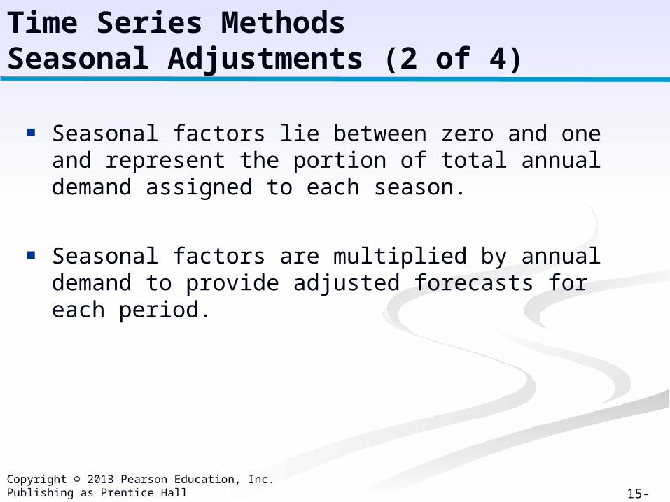
■ Seasonal factors lie between zero and one and represent the portion of total annual demand assigned to each season.

■ Seasonal factors are multiplied by annual demand to provide adjusted forecasts for each period.


15-34


S1 = D1/ D = 42.0/148.7 = 0.28 S2 = D2/ D = 29.5/148.7 = 0.20 S3 = D3/ D = 21.9/148.7 = 0.15 S4 = D4/ D = 55.3/148.7 = 0.37

Table 15.7 Demand for turkeys at Wishbone Farms

Example: Wishbone Farms


15-35


Multiply forecasted demand for an entire year by seasonal factors to determine the quarterly demand.

Forecast for entire year (trend line for data in Table 15.7):

y = 40.97 + 4.30x = 40.97 + 4.30(4) = 58.17 Seasonally adjusted forecasts:

SF1 = (S1)(F5) = (.28)(58.17) = 16.28

SF2 = (S2)(F5) = (.20)(58.17) = 11.63

SF3 = (S3)(F5) = (.15)(58.17) = 8.73

SF4 = (S4)(F5) = (.37)(58.17) = 21.53


15-36


Forecasts will always deviate from actual values. Difference between forecasts and actual values are

referred to as forecast error. We would like forecast error to be as small as

possible. If forecast error is large, either the technique

being used is the wrong one, or the parameters need adjusting.

Measures of forecast errors: Mean Absolute deviation (MAD) Mean absolute percentage deviation

(MAPD) Cumulative error (E bar) Average error, or bias (E)

Forecast AccuracyOverview

15-37


MAD is the average absolute difference between the forecast and actual demand.

The most popular and simplest-to-use measures of forecast error.

Formula:

where:

t the period number D demand in period tt F the forecast for period tt n the total number of periods

D FttMAD n

Forecast AccuracyMean Absolute Deviation (1 of 7)

15-38


Example: PM Computer Services (see Table 15.8).

Compare accuracies of different forecasts using MAD:

53.41 4.8511

D Ft tMAD n


15-39


Table 15.8 Computational values for MAD and error


15-40


The lower the value of MAD relative to the magnitude of the data, the more accurate the forecast.

When viewed alone, MAD is difficult to assess.

MAD must be considered in light of magnitude of the data.


15-41


Can be used to compare the accuracy of different forecasting techniques working on the same set of demand data (PM Computer Services):

Exponential smoothing ( = .50): MAD = 4.04

Adjusted exponential smoothing ( = .50, = .30): MAD = 3.81

Linear trend line: MAD = 2.29

The linear trend line has the lowest MAD; increasing from .30 to .50 improved the smoothed forecast.


15-42


A variation on MAD is the mean absolute percent deviation (MAPD).

Measures the absolute error as a percentage of demand rather than per period.

Eliminates the problem of interpreting the measure of accuracy relative to the magnitude of the demand and forecast values.

Formula:

53.41 .103 or 10.3%520

D Ft tMAPDDt


15-43


MAPD for other three forecasts:

Exponential smoothing ( = .50): MAPD = 8.5%

Adjusted exponential smoothing ( = .50, = .30): MAPD = 8.1%

Linear trend: MAPD = 4.9%


15-44


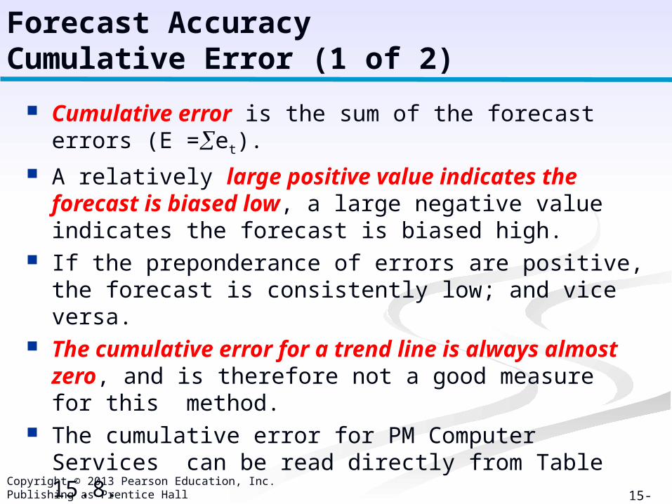
Cumulative error is the sum of the forecast errors (E =et).

A relatively large positive value indicates the forecast is biased low, a large negative value indicates the forecast is biased high.

If the preponderance of errors are positive, the forecast is consistently low; and vice versa.

The cumulative error for a trend line is always almost zero, and is therefore not a good measure for this method.

The cumulative error for PM Computer Services can be read directly from Table 15.8.

E = et = 49.31, indicating the forecasts are frequently below actual demand.

Forecast AccuracyCumulative Error (1 of 2)

15-45


Cumulative error for other forecasts:

Exponential smoothing ( = .50): E = 33.21

Adjusted exponential smoothing ( = .50, =.30):

E = 21.14 Average error (bias) is the per-period average of

cumulative error. Average error for the exponential smoothing

forecast:

A large positive value of average error indicates a forecast is biased low; a large negative error indicates it is biased high.

Forecast AccuracyCumulative Error (2 of 2)

49.31 4.4811

etE n

15-46


Results consistent for all forecasts: Larger value of alpha is preferable. Adjusted forecast is more accurate than

exponential smoothing. Linear trend is more accurate than all the others.

Table 15.9 Comparison of forecasts for PM Computer Services

Forecast AccuracyExample Forecasts by Different Measures

15-47


Exhibit 15.1

Time Series Forecasting Using Excel (1 of 4)

=G21/11

=B3*B8+(1-B3)*C8

=C9+D9 =B9-

E9

=ABS(B9-E9)

=SUM(F9:F20)

15-48


Exhibit 15.2


To access this window, click on “Data” on the toolbar ribbon and then the “Data Analysis” add-in

15-49


Exhibit 15.3


Demand values

a = 0.5

Cells in which the forecasted values will be placed

15-50


Exhibit 15.4


15-51


Exhibit 15.5

Exponential Smoothing Forecast with Excel QM

Click “Add-Ins” to access forecasting macros

Input problem data in cells B7 and B10:B21

15-52


Time Series ForecastingSolution with QM for Windows (1 of 2)

Exhibit 15.6

15-53


Exhibit 15.7

Time Series ForecastingSolution with QM for Windows (2 of 2)

15-54


Time series techniques relate a single variable being forecast to time.

Regression is a forecasting technique that measures the relationship of one variable to one or more other variables.

The simplest form of regression is linear regression.

Regression MethodsOverview

15-55


22

where: mean of the x data

mean of the y data

y a bx

a y bx

xy nxybx nx

xx n

yy n

Linear regression relates demand (dependent variable ) to an independent variable.

Regression MethodsLinear Regression

15-56


State University Athletic Department.

Wins Attendance 4 6 6 8 6 7 5 7

36,300 40,100 41,200 53,000 44,000 45,600 39,000 47,500

x (wins)

y (attendance, 1,000s)

xy

x2

4 6 6 8 6 7 5 7

49

36.3 40.1 41.2 53.0 44.0 45.6 39.0 47.5 346.7

145.2 240.6 247.2 424.0 264.0 319.2 195.0 332.5

2,167.7

16 36 36 64 36 49 25 49

311

Regression MethodsLinear Regression Example (1 of 3)

15-57


49 6.1258

346.9 43.348

(2,167.70 (8)(6.125)(43.34) 4.062 22 (311) (8)(6.125)

43.34 (.406)(6.125) 18.46

Therefore, 18.46 4.06

Attendance forecast for x 7 wins is18.46 4.06(7)

x

y

xy nxybx nx

a y bx

y x

y

46.88 or 46,880


15-58


Figure 15.6Linear regression line


15-59


Correlation is a measure of the strength of the relationship between independent and dependent variables.

Formula:

Value lies between +1 and -1. Value of zero indicates little or no relationship

between variables. Values near 1.00 and -1.00 indicate a strong linear

relationship.

2 22 2

n xy x yrn x x n y y

Regression MethodsCorrelation (1 of 2)

15-60


2 2

(8)(2,167.7) (49)(346.7) .948(8)(311) (49) (8)(15,224.7) (346.7)

r

Value for State University example:

Since the value is close to one, we have evidence of a strong linear relationship.

Regression MethodsCorrelation (2 of 2)

15-61


The coefficient of determination is the percentage of the variation in the dependent variable that results from the independent variable.

Computed by squaring the correlation coefficient, r.

For the State University example:r = .948, r2 = .899

This value indicates that 89.9% of the amount of variation in attendance can be attributed to the number of wins by the team, with the remaining 10.1% due to other, unexplained, factors.

Regression MethodsCoefficient of Determination

15-62


Regression Analysis with Excel (1 of 6)

Exhibit 15.8

=INTERCEPT(B5:B12,A5:A12)

=CORREL(B5:B12,A5:A12)

15-63



Exhibit 15.9

Click on “Insert” to access “Charts”

Click on “Scatter”

15-64


Exhibit 15.10


15-65


Exhibit 15.11


15-66


Exhibit 15.12


15-67


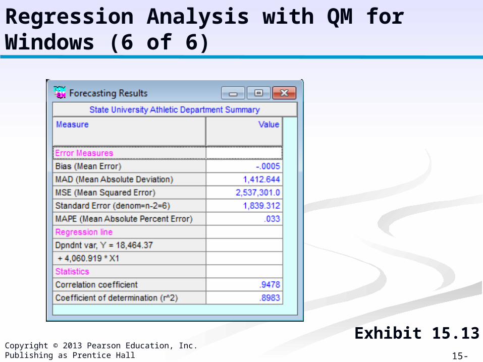
Exhibit 15.13

Regression Analysis with QM for Windows (6 of 6)

15-68


Multiple Regression with Excel (1 of 4)

Multiple regression relates demand to two or more independent variables.

General form:

y = 0 + 1x1 + 2x2 + . . . + kxk

where 0 = the intercept

1 . . . k = parameters representing

contributions of the independent variables

x1 . . . xk = independent variables

15-69


State University example revisited; does the addition of promotional and advertising expenditures to wins improve the prediction of attendance?

Wins Promotion ($) Attendance 4 6 6 8 6 7 5 7

29,500 55,700 71,300 87,000 75,000 72,000 55,300 81,600

36,300 40,100 41,200 53,000 44,000 45.600 39,000 47,500


15-70


Exhibit 15.14


r2, the coefficient of determination

Regression equation coefficients for x1 and x2

15-71


Exhibit 15.15


Includes x1 and x2 columns

15-72


Period Units 1 2 3 4 5 6 7 8

56 61 55 70 66 65 72 75

Problem Statement: For the data below, develop an exponential smoothing

forecast using = .40, and an adjusted exponential smoothing

forecast using = .40 and = .20.

Compare the accuracy of the forecasts using MAD and cumulative error.

Example Problem SolutionComputer Software Firm (1 of 4)

15-73


Step 1: Compute the Exponential Smoothing Forecast.

Ft+1 = Dt + (1 - )Ft

Step 2: Compute the Adjusted Exponential Smoothing

Forecast

AFt+1 = Ft +1 + Tt+1

Tt+1 = (Ft +1 - Ft) + (1 - )Tt


15-74


Period Dt Ft AFt Dt - Ft Dt - AFt 1 2 3 4 5 6 7 8 9

56 61 55 70 66 65 72 75

56.00 58.00 56.80 62.08 63.65 64.18 67.31 70.39

56.00 58.40 56.88 63.20 64.86 65.26 68.80 72.19

5.00

-3.00 13.20

3.92 1.35 7.81 7.68

35.97

5.00

-3.40 13.12

2.80 0.14 6.73 6.20

30.60


15-75


Step 3: Compute the MAD Values

Step 4: Compute the Cumulative Error.

E(Ft) = 35.97

E(AFt) = 30.60

41.97( ) 5.997

37.39( ) 5.347

D Ft tMAD F nt

D AFt tMAD AF nt


15-76


For the following data: Develop a linear regression model Determine the strength of the linear

relationship using correlation. Determine a forecast for lumber given 10

building permits in the next quarter.

Example Problem SolutionBuilding Products Store (1 of 5)

15-77


Quarter

Building Permits, x

Lumber Sales (1,000s of board ft), y

1 2 3 4 5 6 7 8 9

10

8 12 7 9 15 6 5 8 10 12

12.6 16.3 9.3 11.5 18.1 7.6 6.2 14.2 15.0 17.8


15-78


Step 1: Compute the Components of the Linear Regression Equation.

92 9.210

128.6 12.8610

(1,290.3) (10)(9.2)(12.86)2 22 (932) (10)(9.2)

1.25

12.86 (1.25)(9.2)1.36

x

y

xy nxybx nx

a y bx


15-79


Step 2: Develop the Linear regression equation.

y = a + bx, y = 1.36 + 1.25x

Step 3: Compute the Correlation Coefficient.

2 22 2

n xy x yrn x x n y y

22

(10)(1,290.3) (92)(128.6)(10)(932) (92) (10)(1,810.48) (128.6)

.925

r


15-80



Step 4: Calculate the forecast for x = 10 permits.

Y = a + bx = 1.36 + 1.25(10) = 13.86 or 1,386 board ft


15-81


All rights reserved. No part of this publication may be reproduced, stored in a retrieval system, or transmitted, in any form or by any means, electronic, mechanical, photocopying,

recording, or otherwise, without the prior written permission of the publisher. Printed in the United States of America.

Documents

15-1 Copyright © 2013 Pearson Education, Inc. Publishing as Prentice Hall Forecasting Chapter 15