Embed Size (px)
Citation preview

1
14.581 International Trade Class notes on 3/20/20131
Intensive and Extensive Margins in Trade Flows
• With access to micro data on trade flows at the firm-level, a key question to ask is whether trade flows expand over time (or look bigger in the cross-section) along the:
– Intensive margin: the same firms (or product-firms) from country i export more volume (and/or charge higher prices—we can also decompose the intensive margin into these two margins) to country j.
– Extensive margin: new firms (or product-firms) from country i are penetrating the market in country j.
• This is really just a decomposition—we can and should expect trade to expand along both margins.
• Recently some papers have been able to look at this.
– A rough lesson from these exercises is that the extensive margin seems more important (in a purely ‘accounting’ sense, not necessarily a causal sense).
1The notes are based on lecture slides with inclusion of important insights emphasized during the class.
From Bernard, Andrew B., J. Bradford Jensen, et al. Journal of Economic Perspectives 21,no. 3 (2007): 105-30. Courtesy of American Economic Association. Used with permission.
1

Figure 1: Mean value of individual-firm exports (single-region firms, 1992)
Importing country: Belgium Importing country: Switzerland
Belgium Belgium
Germany Germany
Switzerland
0.02
0.46
0.75
1.32
3.45
32.61
Switzerland
0.00
0.10
0.25
0.56
2.32
25.57
Italy Italy
Spain Spain
Importing country: Germany Importing country: Spain
Belgium Belgium
Germany Germany
4,0337.01
1,607.60
0,682.18
0,39Switzerland 1,23 Switzerland 0,180.58
0.00 0,00
Italy Italy
Spain Importing country: Italy Spain
Belgium
Germany
8,96
2,48
0,88
Switzerland 0,51
0,22
Italy
Spain
Figure 1 from Crozet, M., and P. Koenig. "Structural Gravity Equations with Intensive and Extensive Margins." Canadian Journalof Economics/Revue canadienne d'économique 43 (2010): 41–62. © John Wiley And Sons Inc. All rights reserved. This contentis excluded from our Creative Commons license. For more information, see http://ocw.mit.edu/fairuse.
From Bernard, Andrew B., J. Bradford Jensen, et al. Journal of Economic Perspectives 21,no. 3 (2007): 105-30. Courtesy of American Economic Association. Used with permission.
2

Figure 2: Percentage of firms which export (single-region firms, 1992)
Importing country: Belgium Importing country: Switzerland
Belgium Belgium
Germany Germany
92.85 92.59
60.00 61.53
34.21 46.87
Switzerland 23.71Switzerland 38.00
16.66 26.92
0.00 9.37
Italy Italy
Spain Spain
Importing country: Germany Importing country: Spain
Belgium Belgium
Germany Germany
Switzerland
5.00
22.85
32.05
41.93
68.75
100.00
Switzerland
0.00
18.42
25.00
31.11
41.66
80.00
Italy Italy
Spain Spain
Importing country: Italy
Belgium
Germany
80.00
46.15
33.33
Switzerland 25.00
18.18
6.66
Italy
Spain
Figure 2 from Crozet, M., and P. Koenig. "Structural Gravity Equations with Intensive and Extensive Margins." Canadian Journalof Economics/Revue canadienne d'économique 43 (2010): 41–62. © John Wiley And Sons Inc. All rights reserved. This contentis excluded from our Creative Commons license. For more information, see http://ocw.mit.edu/fairuse.
3

Table 2: Decomposition of French aggregate industrial exports (34 industries - 159 countries 1986 to 1992)
All firms Single-region firms > 20 employees > 20 employees (1) (2) (3) (4)
Average Number of Average Number of Shipment Shipments Shipment Shipments
ln (Mkjt/Nkjt) ln (Nkjt) ln (Mkjt/Nkjt) ln (Nkjt) ln (GDPkj) 0.461a
(0.007) 0.417a
(0.007) 0.421a
(0.007) 0.417a
(0.008)
ln (Distj) -0.325a
(0.013) -0.446a
(0.009) -0.363a
(0.012) -0.475a
(0.009)
Contigj -0.064c
(0.035) -0.007 (0.032)
0.002 (0.038)
0.190a
(0.036)
Colonyj 0.100a
(0.032) 0.466a
(0.025) 0.141a
(0.035) 0.442a
(0.027)
Frenchj
N R2
0.213a
(0.029) 23553 0.480
0.991a
(0.028) 23553 0.591
0.188a
(0.032) 23553 0.396
1.015a
(0.028) 23553 0.569
Note: These are OLS estimates with year and industry dummies. Robust stana b cdard errors in parentheses with , and denoting significance at the
1%, 5% and 10% level respectively.
Table 2. Decomposing Spatial Frictions
(5-digit zip code data)
dist dist2 ownzip ownstate constant Adj. R2 N DS value
( ijT )
-0.137
(0.009)
-0.004
(0.001)
1.102
(0.030)
-0.024
(0.007)
-13.393
(0.026)
0.01 1290788 -0.187
# of shipments
( ijN )
# of trading pairs
( F ijN )
# of commodities
( k ijN )
-0.294
(0.002)
-0.159
(0.002)
-0.135
(0.001)
0.017
(0.000)
0.008
(0.000)
0.009
(0.000)
0.883
(0.008)
0.540
(0.007)
0.342
(0.003)
0.043
(0.002)
0.029
(0.002)
0.014
(0.001)
-1.413
(0.007)
-0.888
(0.006)
-0.525
(0.003)
0.10
0.05
0.10
1290840
1290840
1290840
-0.081
-0.059
-0.022
avg. value
( ijPQ )
avg. price
( ijP )
avg. weight
( ijQ )
0.157
(0.008)
-0.032
(0.007)
0.189
(0.011)
-0.021
(0.001)
0.036
(0.001)
-0.058
(0.001)
0.219
(0.028)
-0.115
(0.024)
0.334
(0.037)
-0.067
(0.006)
-0.154
(0.006)
0.087
(0.009)
-11.980
(0.024)
0.021
(0.020)
-12.001
(0.031)
0.00
0.08
0.05
1290788
1290788
1290788
-0.106
0.419
-0.537
Notes:
1. Regression of (log) shipment value and its components from equations (7) and (8) on geographic variables. Dependent variables in left hand
column. Coefficients in right-justified rows sum to coefficients in left justified rows.
2. Standard errors in parentheses.
3. S is the elasticity of trade with respect to distance, evaluated at the sample mean distance of 523 miles. D
© John Wiley And Sons Inc. All rights reserved. This content is excluded from ourCreative Commons license. For more information, see http://ocw.mit.edu/fairuse.
Courtesy of Russell Hillberry and David Hummels. Used with permission.
4
Panel A: Entry of Firms FRA
100000
BELSWI GERITAUNK10000 NET USASPA CAMMOR GREALGDEN SWE CANCOT POR AUT
SEN TUN NOR JAPISR FIN AULSAUIREHOK BENTOG SIN SOUKUW EGYCEN NIG MAL BUK TUR YUGIND1000 TAI BRAMAD MAS ZAI NZE ARGKORMAU VENJOR CHI THAHUN MEXNIAPAKSYR IRQMAYINO CZE CHN USROMA COLCHA ANG BULPAN PERURU KEN PHIRWA ECU IRN ROM GEEBUR LIYSRI SUDPARETH ZIM CUBDOMCOSMOZ LIBTRI BANGUAZAM GHATANELSJAMHON VIENIC
SOM PAP ALB 100 SIE BOL
MAWUGAAFGNEP
10
.1 1 10 100 1000 10000 market size ($ billions)
Panel B: Normalized Entry 5000000 JAP
USA
CAN USR1000000 GER
AUL UNKSWI CHNGEE BUL SPA FRAAUTTAI BRAITA
NZE NORSWEFIN BELYUGNETISR SOUCZEROMVIEGRE DENMEXARGKORINDHOKMAY VENIRESINHUNSAUCHI POR100000 CUB TURCOLALGIRN EGYECU INOSUDCOT PERZIMCAMSYRPHIURU PAN PAK
TAN JORTUNKUWALBTRI COS MOR THADOMSRIETHELSBOL PARBUKSENGUAHON IRQPAPMAS ZAI OMABAN NIAJAM CHAMAL KENSOMTOG ANG LIYMADBENUGA NIC10000 NIGRWA NEPMOZBURCEN ZAM GHA
MAU AFG LIB MAW
SIE1000
.1 1 10 100 1000 10000 market size ($ billions)
Panel C: Sales Percentiles 10
FRA USRCHN GERLIY GEEITA UNK USAINDIRQ EGY BRANIC ALG CZE BELYUGKORNET1 INO MEXBULSWE SPA JAPIRN TURCUB SAUMAW AFG NIAPAK HUNVEN GRE DENFINROMTAI
MORSYR THA SOUNORARGAUL CANPAN PHI SINHOK AUT SWITUN PERMAYIREPORANG COLETHDOM KENKUWCHI VIEZAM BANMOZ ISROMAZAISRIJORCOSCAM NZELIBPAR COTMAU PAPGHA GUAELS SUDECU BUR MALUGABUK ALBHONMADNEP TRI ZIMTAN URUMASSENNIG BEN JAMTOGRWA.1 SIE SOM BOLCEN CHA
.01
.001 .1 1 10 100 1000 10000
market size ($ billions)
2 Helpman, Melitz and Rubenstein (QJE, 2008)
• What does the difference between intensive and extensive margins imply for the estimation of gravity equations?
– Gravity equations are often used as a tool for measuring trade costs and the determinants of trade costs—we will see an entire lecture on
entry
nor
mal
ized
by
Fren
ch m
arke
t sha
re
# fir
ms
sellin
g in
mar
ket
perc
entil
es (2
5, 5
0, 7
5, 9
5) b
y m
arke
t ($
milli
ons)
© The Econometric Society. All rights reserved. This content is excluded from ourCreative Commons license. For more information, see http://ocw.mit.edu/fairuse.
5

estimating trade costs later in the course, and gravity equations will loom large.
• HMR (2008) started wave of thinking about gravity equation estimation in the presence of extensive/intensive margins.
– They use aggregate international trade (so this paper doesn’t technically belong in a lecture on ‘firm-level trade empirics’ !) to explore implications of a heterogeneous firm model for gravity equation estimation.
– The Melitz (2003) model—which you’ll see properly next week—is simplified and used as a tool to understand, estimate, and correct for biases in gravity equation estimation.
2.1 HMR (2008): Zeros in Trade Data
• HMR start with the observation that there are lots of ‘zeros’ in international trade data, even when aggregated up to total bilateral exports.
– Baldwin and Harrigan (2008) and Johnson (2008) look at this in a more disaggregated manner and find (unsurprisingly) far more zeros.
• Zeros are interesting.
• But zeros are also problematic.
– A typical analysis of trade flows is based on the gravity equation (in logs), which can’t incorporate Xij = 0
– Indeed, other models of the gravity equation (Armington, Krugman, Eaton-Kortum) don’t have any zeros in them (due to CES and unbounded productivities and finite trade costs).
6

FIGURE I Distribution of Country Pairs Based on Direction of Trade
Note. Constructed from 158 countries.
FIGURE II Aggregate Volume of Exports of All Country Pairs and of Country Pairs That
Traded in Both Directions in 1970
2.2 A Gravity Model with Zeroes
• HMR work with a multi-country version of Melitz (2003)—similar to Chaney (2008).
• Set-up:
– Monopolistic competition, CES preferences (ε), one factor of production (unit cost cj ), one sector.
100
90
80
70
60
40
50
30
20
0
10
Perc
en
t o
f co
un
try p
air
s
1970
1972
1974
1976
1978
1980
1982
1984
1986
1988
1990
1992
1994
1996
No Trade
Trade in one direction only
Trade in both directions
Image by MIT OpenCourseWare.
6,000
5,000
4,000
3,000
2,000
1,000
0
1970
1972
1976
1980
1984
1988
1992
1996
1974
1978
1982
1986
1990
1994
Year
Bill
ions
of 20
00 U
.S.
dolla
rs
Trade in both directions in 1970All country pairs
Image by MIT OpenCourseWare.
7

– Both variable (iceberg τij ) and fixed (fij ) costs of exporting.
– Heterogeneous firm-level productivities 1/a drawn from truncated Pareto, G(a).
• Some firms in j sell in country i iff a ≤ aij , where the cutoff productivity (aij ) is defined by: 1−ε
τij cj aijκ1 Yi = cj fij (1)
Pi
• HMR (2008) derive a gravity equation, for those observations that are non-zero, of the form:
ln(Mij ) = β0 + αi + αj − γ ln dij + wij + uij (2)
• Where:
– Mij is imports
– dij is distance
– wij is the ‘augmented’ part, which is a term accounting for selection.
– Mij = 0 is possible here (even with CES preferences and finite variable trade costs) because it is assumed that each country’s firms have productivities drawn from a bounded (truncated Pareto) distribution.
2.3 Two Sources of Bias
• The HMR (2008) theory suggests (and solves) two sources of bias in the typical estimation of gravity equations (which neglects wij ).
• First: Omitted variable bias due to the presence of wij :
– In a model with heterogeneous firm productivities and fixed costs of exporting (i.e. a Melitz (2003) model), only highly productive firms will penetrate distant markets.
– So distance (dij ) does two things: it raises the price at which any firm can sell (thus reducing demand along the intensive margin) in, and it changes the productivity (and hence the price and hence the amount sold) of the firms entering, a distant market.
– This means that dij is correlated with wij .
– Therefore, if one aims to estimate γ but neglects to control for wij
the estimate of γ will be biased (due to OVB).
)
8

• The HMR (2008) theory suggests (and solves) two sources of bias in the typical estimation of gravity equations (which neglects wij ).
• Second: A selection effect induced by only working with non-zero trade flows:
– HMR’s gravity equation, like those before it, can’t be estimated on the observations for which Mij = 0.
– The HMR theory tells us that the existence of these ‘zeros’ is not as good as random with respect to dij , so econometrically this ‘selection effect’ needs to be corrected/controlled for.
– Intuitively, the problem is that far away destinations are less likely to be profitable, so the sample of zeros is selected on the basis of dij .
– This calls for a standard Heckman (1979) selection correction.
2.4 HMR (2008): Two-step Estimation
1. Estimate probit for zero trade flow or not:
• Include exporter and importer fixed effects, and dij .
• Can proceed with just this, but then identification (in Step 2) is achieved purely off of the normality assumption.
• To ‘strengthen’ identification, need additional variable that enters Probit in step 1, but does not enter Step 2.
• Theory says this should be a variable that affects the fixed cost of exporting, but not the variable cost.
• HMR use Djankov et al (QJE, 2002)’s ‘entry regulation’ index. Also try ‘common religion dummy.’
2. Estimate gravity equation on positive trade flows:
• Include inverse Mills ratio (standard Heckman trick) to control for selection problem (Second source of bias)
• Also include empirical proxy for wij based on estimate of entry equation in Step 1 (to fix First source of bias).
9

Crozet and Koenig (CJE, 2010)
• CK (2010) conduct a similar exercise to HMR (2008), but with French firm-level data.
3
Distance
Land border
Island
Landlock
Legal
Language
Colonial ties
Currency union
FTA
Religion
WTO (none)
WTO (both)
Observations R2
-1.176**(0.031)
-0.263**(0.012)
-1.201**(0.024)
-0.246**(0.008)
-1.200**(0.024)
-0.246**(0.008)
0.458**(0.147)
-0.148**(0.047)
0.366**(0.131)
-0.146**(0.032)
0.364**(0.131)
-0.146**(0.032)
-0.391**(0.121)
-0.136**(0.032)
-0.381**(0.096)
-0.140**(0.022)
-0.378**(0.096)
-0.140**(0.022)
-0.087**-0.561**(0.188)
-0.072(0.045)
-0.582**(0.148)
-0.087**(0.028)
-0.581**(0.147) (0.028)
0.486**(0.050)
0.038**(0.014)
0.406**(0.040)
0.029**(0.009)
0.407**(0.040)
0.028**(0.009)
1.176**(0.061)
0.113**(0.016)
0.207**(0.047)
0.109**(0.011)
0.203**(0.047)
0.108**(0.011)
1.299**(0.120)
0.128(0.117)
1.321**(0.110)
0.114(0.082)
1.326**(0.110)
0.116(0.082)
1.364**(0.255)
0.190**(0.052)
1.395**(0.187)
0.206**(0.026)
1.409**(0.187)
0.206**(0.026)
0.759**(0.222)
0.494**(0.020)
0.996**(0.213)
0.497**(0.018)
0.976**(0.214)
0.495**(0.018)
0.102(0.096)
0.104**(0.025)
-0.018(0.076)
0.099**(0.016)
-0.038(0.077)
0.098**(0.016)
-0.068(0.058)
-0.056**(0.013)
0.303**(0.042)
0.093**(0.013)
11,1460.709
24,6490.587
110,6970.682
248,0600.551
110,6970.682
248,0600.551
Variablesmij
Tij mij
Tij mij
Tij
(Porbit) (Porbit) (Porbit)
1986 1980's
Notes. Exporter, importer, and year fixed effects. Marginal effects at sample means and pseudo R2 reported for Probit. Robust standard errors (clustering by country pair).+ Significant at 10%* Significant at 5%** Significant at 1%
Benchmark Gravity and Selection into Trading Relationship
Image by MIT OpenCourseWare.
Baseline Results
Observations R2
Distance
Island
Landlock
Legal
Language
Colonial ties
Currency union
FTA
Religion
Regulationcosts
R costs (days& proc)
Land border
0.840**(0.043)0.240*
(0.099)
-0.813(0.049)0.871
(0.170)
-0.203(0.290)-0.347*(0.175)0.431**
(0.065)-0.030(0.087)0.847**
(0.257)1.077**
(0.360)0.124
(0.227)0.120
(0.136)
6,602
-0.755**(0.070)0.892**0.170)
-0.161(0.259)-0.352+(0.187)0.407**
(0.065)-0.061(0.079)0.853**
(0.152)1.045**
(0.337)-0.141(0.250)0.073
(0.124)
6,6020.704
1.107**
-0.789**(0.088)0.863**
(0.170)-0.197(0.258)-0.353+(0.187)0.418**
(0.065)-0.036(0.083)0.838**
(0.153)
(0.346)0.065
(0.348)0.100
(0.128)
6,6020.706
(0.036)
-0.061*(0.031)
-0.108**
-0.213**(0.016)
-0.087(0.072)
-0.173*(0.078)
-0.053(0.050)
0.049**(0.019)
0.101**(0.021)
-0.009(0.130)
0.216**(0.038)
0.343**(0.009)
0.141**(0.034)
12,1980.573
1.534**
-1.146(0.100)
-0.216+(0.124)
-1.167**(0.040)0.627**
(0.165)
-0.553*(0.269)-0.432*(0.189)0.535**
(0.064)0.147+
(0.075)0.909**
(0.158)
(0.334)0.976**
(0.247)0.281*
(0.120)
6,6020.693
(0.052)-0.847**
(0.166)0.845**
(0.258)-0.218
(0.187)-0.362+
(0.064)0.434**
(0.077)-0.017
(0.148)0.848**
(0.333)1.150**
(0.197)0.241
(0.120)0.139
0.7016,602
(0.540)3.261**
(0.170)-0.712**
(0.017)0.060**
0.882**(0.209)
Variables (Probit)Tij Benchmark NLS Polynomial
50 bins 100 bins
Indicator variables
mij
1986 reduced sample
Notes: Exporter and importer fixed effects. Marginal effects at sample means and pseudo R2 reportedfor Probit. Regulation costs are excluded variables in all second stage specifications. Bootstrapped standarderrors for NLS; robust standard errors (clustering by country pair) elsewhere.+Significant at 10%.*Significant at 5%.**Significant at 1%.
*ij
*ij*ij
*ωij(from )δ
2
3
*ijη
Image by MIT OpenCourseWare.
10

– This is attractive—after all, the main point that HMR (2008) is making is that firm-level realities matter for aggregate flows.
• CK’s firm data has exports to foreign countries in it (CK focus only on adjacent countries: Belgium, Switzerland, Germany, Spain and Italy).
3.1 CK (2010): Identification
• But interestingly, CK also know where the firm is in France.
• So they try to separately identify the effects of variable and fixed trade costs by assuming:
– Variable trade costs are proportional to distance. Since each firm is a different distance from, say, Belgium, there is cross-firm variation here.
– Fixed trade costs are homogeneous across France for a given export destination. (It costs just as much to figure out how to sell to the Swiss whether your French firm is based in Geneva or Normandy).
3.2 CK (2010): The model and estimation
• The model is deliberately close to Chaney (2008), which is a particular version of the Melitz (2003) model but with (unbounded) Pareto-distributed firm productivities (with shape parameter γ). We will see this model in detail in the next lecture.
• In Chaney (2008) the elasticity of trade flows with respect to variable trade costs (proxies for by distance here, if we assume τij = ij whereθDδ
D = distance) can be subdivided into the:
EXTj– Extensive elasticity: ε = −δ [γ − (σ − 1)]. CK estimate this by Dij
regressing firm-level entry (ie a Probit) on firm-level distance Dij and a firm fixed effect. This is analogous to HMR’s first stage.
INTj– Intensive elasticity: ε = −δ(σ − 1). CK estimate this by re-Dij
gressing firm-level exports on firm-level distance Dij and a firm fixed effect. This is analogous to HMR’s second stage.
• Recall that γ is the Pareto parameter governing firm heterogeneity.
• The above two equations (HMR’s first and second stage) don’t separately identify δ, σ and γ.
– So to identify the model, CK bring in another equation which is the slope of the firm size (sales) distribution.
11

= λ(ci)−[γ−(σ−1)]– In the Chaney (2008) model this will behave as: Xi , where ci is a firm’s marginal cost and Xi is a firm’s total sales.
– With an Olley and Pakes (1996) TFP estimate of 1/ci, CK estimate [γ − (σ − 1)] and hence identify the entire system of 3 unknowns.
12

3.3 CK (2010): Results (each industry separately)
3.4 CK (2010): Results (do the parameters make sense?)
3.5 CK (2010): Results (what do the parameters imply about margins?)
Figure 4: The estimated impact of trade barriers and distance on trade margins, by industry
1011
1314151617181920212223242527282930313233344445464748495051525354
Glass
Textile
Rubber
Iron and steelSteel processingMetallurgyMineralsCeramic and building mat.
Speciality chemicalsPharmaceuticalsFoundryMetal work
Industrial equipmentMining / civil egnring eqpmtOffice equipmentElectrical equipmentElectronical equipment Domestic equipmentTransport equipmentShip buildingAeronautical buildingPrecision instruments
Leather productsShoe industryGarment industryMechanical woodworkFurniturePaper & CardboardPrinting and editing
Plastic processingMiscellaneous
Chemicals
Agricultural machinesMachine tools
-5.51*-1.5*-2.14*-2.98*-2.63*-2.33*-1.81*-0.97*-1.19*-1.72*-1.19*-2.06*-1.29*-1.25*-1.37*-0.52*-0.8*-0.77*-0.94*-1.4*-3.69*-0.78*-1.07*-1.17*-1.24*-0.42*-0.33*-2.14*-1.43*-1.45*-1.4*-1.26*-1.24*-0.91*
-1.41
-1.71*-0.99*-0.73*-0.91*-0.76*-0.58*
-0.76*0.34*-0.14-0.85*-0.36*-0.57*-0.48*-0.48*-0.46*-1.02-0.14-0.24*-0.14*-0.55*-2.67*-0.130.08 -0.3*-0.44*-0.29*0.13-0.2*-0.37*0.76*0.7*0.8*0.51*-0.33*
-0.53
-1.36-1.74-1.85-2.86
-2.13-1.97
-1.39-1.09
-2.37-1.4
-2.39-2.43
-1.97-2.47
-1.57-1.9
-1.63-2.34
-2.13
-1.52-2.23
-1.63-3.27
-1.63-1.37
-1.04-2.3
-2.25-1.5
-1.24-1.76
-1.6-2.52
-1.22
1.98 1.62 2.785.1 4.36 0.292.82 1.97 0.764.11 2.25 0.722.76 1.79 0.952.84 1.7 0.82
1.89 1.8 0.952.13 1.74 0.46
4.68 3.31 0.373.48 2.05 0.343.31 1.92 0.623.92 2.45 0.333.21 2.24 0.392.86 1.96 0.48
2.34 1.71 0.332.51 1.37 0.383.69 2.46 0.385.53 5.01 0.67
1.84 1.47 0.642.53 1.9 0.497.31 6.01 0.06
1.65 1.15 1.293.04 1.79 0.473.71 2.95 0.392.46 2.22 0.576.93 5.41 0.182.7 2.11 0.461.92 1.7 0.47
3.09 2.25 0.58-1.86Tread weighted mean
The Structural Parameters of the Gravity Equation (Firm-level Estimations)
Code IndustryP[Export > 0]
-δγExport value
-δ(σ−1)Pareto#
−[γ−(σ−1)] σ δγ
*,** and ***denote significance at the 1%, 5% and 10% level respectively. #: All coefficients in this column are significant at the 1% level. Estimations include the contiguity variable.
Image by MIT OpenCourseWare.
Figure 3: Comparison of our results for σ and δ with those of Broda and Weinstein (2003)
Bro
da a
nd W
eins
tein
's s
igm
a (
log
scal
e)
48 30
44
45
4549
102820181722
21 51
1424
5325
31
20
52
11
50
13 23
32
Sigma (log scale)1 2 3 4 5
10
20
30
40
US-C
anad
a fr
eigh
t ra
te (
log
scal
e)
.5
1
2
Delta (log scale)
1.5
1 2 3
5252
1150
21115021
2923
302431
452554
25 5144
32
13 1516 17
14
48
10
22
Image by MIT OpenCourseWare.
ShoeElectronical equip.MiscellaneousDomestic equip.Speciality chemicalsTextileMetal workLeather productPlastic processingRubberIndustrial equip.Machine toolsMining/Civil egnring equip.Transport equip.Printing and editingFurniturePaper and cardboardSteel processingFoundryChemicalsAgricultural mach.Mechanical woodworkMetallurgyGlassCeram. and building mat.MineralsShip buildingIron and Steel
Intensive Margin -δ(σ-1)
Extensive Margin −δ(γ−(σ−1))
6 4 2 0
Impact of Distance on Trade Margins
Image by MIT OpenCourseWare.
13

4 Eaton, Kortum and Kramarz (2009)
• EKK (2009) construct a Melitz (2003)-like model in order to try to capture the key features of French firms’ exporting behavior:
– Whether to export. (Simple extensive margin).
– Which countries to export to. (Country-wise extensive margins).
– How much to export to each country. (Intensive margin).
• They uncover some striking regularities in the firm-wise sales data in (multiple) foreign markets.
– These ‘power law’ like relationships occur all over the place (Gabaix (ARE survey, 2009)).
– Most famously, they occur for domestic sales within one market.
– In that sense, perhaps it’s not surprising that they also occur market by market abroad. (At the heart of power laws is scale invariance.)
Intensive Margin −(σ-1)
Extensive Margin −(γ−(σ−1))
Mechanical woodworkTextileChemicalsMiscellaneousIron and SteelSpeciality chemicalsElectronical equip.Printing and editingDomestic equip.Leather productPlastic processingCeram. and bulding mat.MetallurgyGlassMining/Civil egnring equip.FurnitureIndustrial equip.Agricultural mach.Metal workTransport equip.Paper and cardboardMineralsMachine toolsFoundrySteel processingShip buildingRubberShoe
02468
Impact of a Tariff on Trade Margins
Image by MIT OpenCourseWare.
14
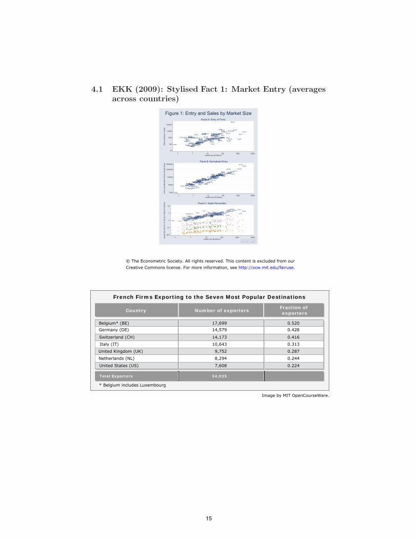
French Firms Exporting to the Seven Most Popular Destinations
Belgium* (BE)Germany (DE)
Switzerland (CH)
Italy (IT)
United Kingdom (UK)
Netherlands (NL)
United States (US)
Total Exporters
* Belgium includes Luxembourg
Number of exporters
17,69914,579
14,173
10,643
9,752
8,294
7,608
34,035
Fraction of exporters
0.5200.428
0.416
0.313
0.287
0.244
0.224
Country
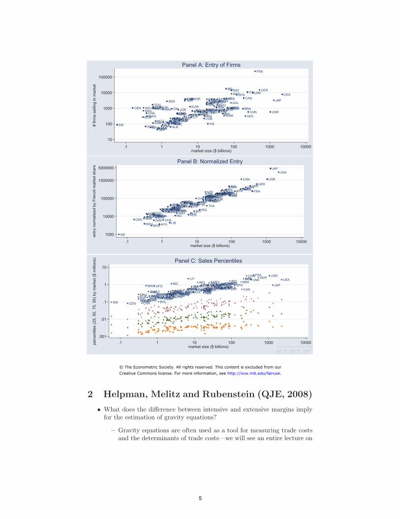
4.1 EKK (2009): Stylised Fact 1: Market Entry (averages across countries)
Figure 1: Entry and Sales by Market Size Panel A: Entry of Firms
FRA
100000
BELSWI GER NET ITAUNK10000 SPA USA
CAMMOR PORALG SWE CANCOT AUT SEN TUN GRE DENNOR JAPISR FIN AULSAUIREHOKTOG SIN SOU
CEN NIG BEN KUW TUR YUGTAIKOR BRA OMA SYR IRQMAYINO CZE CHN USR
MAL BUK ZAI EGY IND1000
MAU MAD MAS NZE VEN ARGJOR CHI THAHUN MEXNIAPAK
RWA ECUKEN IRN ROM GEE COL
BUR LIY CHA ANG BULURU PAN PHIPER
SRI SUD CUBPAR GHATAN
ETHDOMZIMCOSMOZ LIBTRI BANGUAZAM HONJAMELSNIC VIE MAWUGA
100 SIE BOLSOM PAP ALBAFGNEP
10
.1 1 10 100 1000 10000 market size ($ billions)
Panel B: Normalized Entry 5000000 JAP
USA
CAN USR1000000 GER
AUL UNKSWI CHNGEEAUTTAI BRAITABUL SPA FRANZE NORSWEISR SOUFIN BELYUGNETCZEARG GRE DENMEXROMKORHOKVIE INDMAY VENIRESINHUNSAUCHI POR100000 CUBCOLALGTUR
ZIMSUDCAMCOT PHIPERIRN EGY ALBTRI URUCOS MORPAK
ECU INOSYRPAN
TAN JORTUNKUW THADOMSRIETHELSBUKSENHONOMABOL PARGUA IRQPAP ZAI BAN NIA CHAMALMAD KEN
MASJAMSOMTOG ANG LIY UGA NIC
CEN ZAM GHA 10000 NIGRWABENMOZNEP
BUR LIBMAU AFGMAW
1000 SIE
.1 1 10 100 1000 10000 market size ($ billions)
Panel C: Sales Percentiles 10
CHNFRA USRGERLIY GEEITA UNK USAINDEGY MAW AFG NIAPAK HUNVEN ARGAUL
IRQ ALG KOR BRA1 NIC INOTURCZEMEXBULBELYUGNETSPA JAPIRN SWECUB SAU
COL TAIROMTHA NORMORSYR PERIREPORSINGRE DENSOUFINAUT SWIPAN PHI HOK CAN
MOZ ETHANG TUNKEN CHI ISRVIE
BUR UGA TANALB URU ZAM BAN KUW MAYDOMJOR NZE
MAL BUKSEN MAU GHALIBPARZAIELSSRIOMACOSSUDECUCAMCOTPAP GUAMADNEP TRI ZIMMAS HONNIG TOG JAMBENRWA.1 SIE SOM BOLCEN CHA
.01
.001 .1 1 10 100 1000 10000
market size ($ billions)
perc
entil
es (2
5, 5
0, 7
5, 9
5) b
y m
arke
t ($
milli
ons)
entry
nor
mal
ized
by
Fren
ch m
arke
t sha
re
# fir
ms
sellin
g in
mar
ket
© The Econometric Society. All rights reserved. This content is excluded from ourCreative Commons license. For more information, see http://ocw.mit.edu/fairuse.
Image by MIT OpenCourseWare.
15

4.2 EKK (2009): Stylised Fact 2: Sales Distributions (across
all firms)
4.3 EKK (2009): Stylised Fact 3: Export Participation
and Size in France
4.4 EKK (2009): Stylised Fact 4: Export Intensity
Export string
9,260 4,532
BE* 3,988 1,700 4.417BE-DE 863 1,274 912BE-DE-CH 579 909 402BE-DE-CH-IT 330 414 275BE-DE-CH-IT-UK 313 166 297BE-DE-CH-IT-UK-NL 781 54 505BE-DE-CH-IT-UK-NL-US 2,406 15 2,840
9,648Total
* The string "BE" means selling to Belgium but no other among the top 7, "BE-DE" means selling to Belgium and Germany but no other, etc.
DataUnder
independenceModel
French Firms Selling to Strings of Top Seven Countries
Number of French exporters
Image by MIT OpenCourseWare.
1000100101
.1
.001.01
1000100101
.1
.001.01
.00001 .00001.0001 .0001.001 .001.01 .01.1 .11 1
Fraction of firms selling at least that much
Sal
es in
mar
ket
rela
tive
to m
ean
Sales Distributions of French Firms
Belgium-Luxembourg France
United StatesIreland
Image by MIT OpenCourseWare.
1
1
2
2
3
34
45
56
6798
798123456789
123456789
123456789
123456789
123456789
123456789
123456789
123456789
123456789
123456789
123456789
123456789
123456789
123456789
123456789123456789
123456789
123456789
123456789
123456789
123456789123456789
123456789123456789123456789
123451234512345123451234512345
1234512345
12345123451234512345
110 1081051000
1000
100
10
11 10 100 1000 10000 10000 500000
#Firms selling to k or more market
Sales and # Penetrating Multiple Markets
NEPAFG
AFGBRIJANJAW
TANTRYCHA
DELBRABRASEBSEB
FRA
AFGPANLMBNEP AFGPAN
PANCHADELDELBRALMB
NEPAFGPAN
CHACHACHA
CHACHACHACHA
DELDELDELDEL
BRASEBLMBNEPAFG
PANCHADELBRASEB
LMBLMB
LMBLMB
LMBNEPAFGPANCHADELBRASEBSEB LMB
NEPAFGPANCHADELBRASEBLMBNEPAFG
PANCHACHA DELBRASEBLMBNEPAFGPANCHADELBRASEB
LMBNEPAFG
PANCHADELBRASEBLMBNEPAFG
PANCHADELBRASEBLMBNEPAFG
PANCHADELBRASEBLMBNEPNEPAFG
PAN
20 100 1000 10000 100000 500000
.1
1
10
100
1000
10000
#Firms selling in the market
Distribution of Sales and Market Entry
1000
1000
100
10
1
1 2 4 8 16 32 64 128Minimum number of markets penetrated
Sales and Markets Penetrated
Aver
age
sale
in F
ranc
e (
$ m
illio
ns)
NEP
AFGPAN
FRA
LMBNEPAFG
PANCHADELBRASEBLMBNEPAFG
PANCHADEL
BRA
SEBLMBNEP
CHADELBRASEBSEB
DELBRABRASEB
AFGBRALMBNEPAFG
PANCHADELBRALMBNEPAFG
PANCHADELBRASEB
AFGBRALMBNEPAFG
PANCHABRASEB SEBSEBSEBSEB
AFGBRALMBNEPAFG
PANCHADELBRASEBLMBNEP
PANCHADELBRASEBSEB
AFGBRALMBAFGPANCHADELBRALMBNEPAFG
PANCHADELBRASEBLMB
AFGBRALMBNEPAFG
PANCHADELBRASEBLMBAFGPANCHADELBRA
LMB
NEPPANCHADEL
1000
100
10
120 100 1000 10000 100000 500000
#Firms selling in the market
Sales and # Selling to a Market
Aver
age
sale
s in
Fra
nce
($ m
illio
ns)
Aver
age
sale
in F
ranc
e ($
mill
ions
)Pe
rcen
tiles
(25
, 50
, 75
, 95
) in
Fr
ance
($
mill
ions
)
Sales in France and Market Entry
Image by MIT OpenCourseWare.
16

• EKK (2009) therefore add some features to Melitz (2003) in order to bring this model closer to the data.
• Most of these will take the flavor of ‘firm-specific shocks/noise’.
– The shocks smooths things out, allows for unobserved heterogeneity, and answer the structural econometrician’s question of “where does your regression’s error term come from?”.
• The remaining slides describe some of the features of the EKK model, and how the model matches the data. I include them here just for your interest as they won’t make much sense until you’ve learned the Melitz (2003) model—see the next lecture!
• Shocks:
– Firm (ie j)-specific productivity draws (in country i): zi(j). This is Pareto with parameter θ.
– Firm-specific demand draw αn(j). The demand they face in market −(σ−1) n is thus: Xn(j) = αn(j)fXn P
p n
, where f will be defined
shortly.
– Firm-specific fixed entry costs Eni(j) = εn(j)EniM(f), where εn(j) is the firm-specific ‘fixed exporting cost shock’, Eni is the fixed exporting term that appears in Melitz (2003) or HMR (2008) (ie con
1−(1−f)1−1/λ
stant across firms). And M(f) = , which, following 1−1/λ
Arkolakis (2008), is a micro-founded ‘marketing’ function that captures how much firms have to pay to ‘access’ f consumers (this is a choice variable).
– EKK assume that g(α, ε) can take any form, but it needs to be the same across countries n, iid across firms, and within firms independent from the Pareto distribution of z.
wiτij• The entry condition is similar to Melitz (2003). Enter if cost cni(j) = zi (j) satisfies:
1/(σ−1)ηXn Pn
c ≤ c̄ ni(η) ≡ (3)σEni m̄
(j) ≡ αn (j)– Here ηn .εn(j)
– And Xn is total sales in n, Pn is the price index in n, and m̄ is the (constant) markup.
)
( )
17

• Integrating this over the distribution g(η) we know how much entry (measure of firms) there is:
κ2 πniXnJni = (4)
κ1 σEni
• This therefore agrees well with Fact 1 (normalized entry is linear in Xn).
Figure 1: Entry and Sales by Market Size Panel A: Entry of Firms
FRA
100000
BELSWI GER NETSPA USA
ITAUNK10000 CAM AUTCOTMOR PORALG SWE CANTUN GRE DEN JAPSEN NORISRHOK FIN AULSAUIRETOG SIN SOUEGYCEN BEN KUW TUR YUGIND1000 NIG MALMADBUKMAS ZAI JOR CHI THAHUN MEX TAIKOR BRANZE VEN ARGMAU NIA MAYINOOMA PAK COL CZE CHN USRCHA SYR IRQ
BUR ECU LIY ANGURU PHI BULPAN PERKENRWA IRN ROM GEE
PARSRI SUD CUBETHDOMZIM ZAM GHATANHON
COSTRI BANMOZ LIBGUAJAMELSNIC VIE
UGA 100 SIE BOLSOM PAP ALBMAW AFGNEP
10
.1 1 10 100 1000 10000 market size ($ billions)
Panel B: Normalized Entry 5000000 JAP
USA
CAN USR1000000 GER
AUL UNKSWI CHNGEEAUTTAI BRAITABUL SPA FRANZE NORSWEISR SOUFINARGBELYUGNETCZEROM CHI PORIRESINVIEGREHUNHOKSAUVEN
DENMEX KORINDMAY100000 CUB TUR ZIMCAMSYR
COLIRN ALGEGY ALB PANMORPAK
SUDECU PHIPER INOCOT TRI URUCOS KUW
BUKPAPSENHONOMABAN TANDOMJORTUN THASRIETHELSBOL PAR
SOMTOG ANG LIY GUA IRQZAI NIAMASJAM
CHAMALMAD KENRWABENUGA NICNEP CEN ZAM GHA
10000 NIG MOZBUR LIBMAU AFGMAW
1000 SIE
.1 1 10 100 1000 10000 market size ($ billions)
Panel C: Sales Percentiles 10
FRA LIY ITA UNK
CHN USR USAGERGEE
INDIRQ EGY BRA CUB VENNIC ALG YUGKOR1 IRN BUL SPAINO CZEMEXBELSWENET JAPMAW AFG NIAPAK GRE
HUNSAUTURDENFINROMTAI TUN PERMAYIREPOR
ARGAUL MOZ CHI
THA NORPAN SOU ZAM ETHDOMOMABAN KENKUW ISR
MORSYRPHI SINHOK AUT SWI CANANG COLVIEZAISRIJORCOSCAM NZE
MAL BUKMAS ALBHONGHA GUA COTPARMAU PAP LIBELS SUDECUNEP TRI ZIM
TOGMAD TAN URU
RWA BUR UGA SENNIG BEN JAM
.1 SIE SOM BOLCEN CHA
.01
.001 .1 1 10 100 1000 10000
market size ($ billions)
• The firm sales (conditional on entry) condition is similar to Arkolakis (2008):
λ(σ−1) −(σ−1)c c
Xni(j) = ε 1 − σEni. (5) c̄ ni(η) c̄ ni(η)
• There is more work to be done, but one can already see that this will look a lot like a Pareto distribution (c is Pareto, so c to any power is also Pareto) in each market (as in Figure 2).
λ(σ−1) c• But the 1 − will cause the sales distribution to deviate c̄ni(η)
from Pareto in the lower tail (also as in Figure 2).
perc
entil
es (2
5, 5
0, 7
5, 9
5) b
y m
arke
t ($
milli
ons)
entry
nor
mal
ized
by
Fren
ch m
arke
t sha
re
# fir
ms
sellin
g in
mar
ket
© The Econometric Society. All rights reserved. This content is excluded from ourCreative Commons license. For more information, see http://ocw.mit.edu/fairuse.
( ) ( )
( )
18

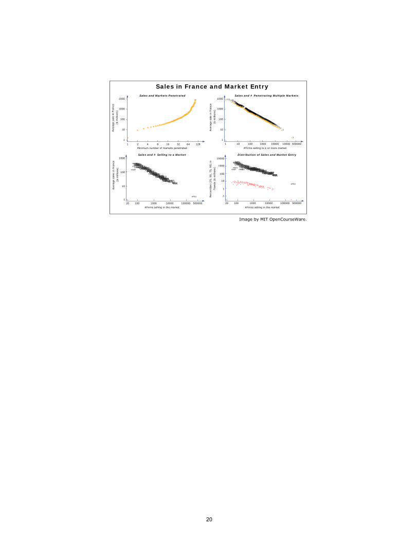
• The amount of sales in France conditional on entering market n can be shown to be:
/λ/θ λαF (j) NnF ηn(j)θXFF (j)|n = 1 − vnF (j)
λ//
ηn(j) NFF ηF (j)
−1//θ θ NnF κ2 ¯ × vnF (j)
−1// XFF .
NFF κ1
• Since NnF /NFF is close to zero (everywhere but in France) the dependence of this on NnF is Pareto with slope −1/θe. As in Figure 3.
[ ( ) ( ) ]( )
1000100101
.1
.001.01
1000100101
.1
.001.01
.00001 .00001.0001 .0001.001 .001.01 .01.1 .11 1
Fraction of firms selling at least that much
Sal
es in
mar
ket
rela
tive
to m
ean
Sales Distributions of French Firms
Belgium-Luxembourg France
United StatesIreland
Image by MIT OpenCourseWare.
19
1
1
2
2
3
34
45
56
6798
798123456789
123456789
123456789
123456789
123456789
123456789
123456789
123456789
123456789
123456789
123456789
123456789
123456789
123456789
123456789123456789
123456789
123456789
123456789
123456789
123456789123456789
123456789123456789123456789
123451234512345123451234512345
1234512345
12345123451234512345
1101081051000
1000
100
10
11 10 100 1000 10000 10000 500000
#Firms selling to k or more market
Sales and # Penetrating Multiple Markets
NEPAFG
AFGBRIJANJAW
TANTRYCHA
DELBRABRASEBSEB
FRA
AFGPANLMBNEP AFGPAN
PANCHADELDELBRALMB
NEPAFGPAN
CHACHACHA
CHACHACHACHA
DELDELDELDEL
BRASEBLMBNEPAFG
PANCHADELBRASEB
LMBLMB
LMBLMB
LMBNEPAFGPANCHADELBRASEBSEB LMB
NEPAFGPANCHADELBRASEBLMBNEPAFG
PANCHACHA DELBRASEBLMBNEPAFGPANCHADELBRASEB
LMBNEPAFG
PANCHADELBRASEBLMBNEPAFG
PANCHADELBRASEBLMBNEPAFG
PANCHADELBRASEBLMBNEPNEPAFG
PAN
20 100 1000 10000 100000 500000
.1
1
10
100
1000
10000
#Firms selling in the market
Distribution of Sales and Market Entry
1000
1000
100
10
1
1 2 4 8 16 32 64 128Minimum number of markets penetrated
Sales and Markets Penetrated
Aver
age
sale
in F
ranc
e (
$ m
illio
ns)
NEP
AFGPAN
FRA
LMBNEPAFG
PANCHADELBRASEBLMBNEPAFG
PANCHADEL
BRA
SEBLMBNEP
CHADELBRASEBSEB
DELBRABRASEB
AFGBRALMBNEPAFG
PANCHADELBRALMBNEPAFG
PANCHADELBRASEB
AFGBRALMBNEPAFG
PANCHABRASEB SEBSEBSEBSEB
AFGBRALMBNEPAFG
PANCHADELBRASEBLMBNEP
PANCHADELBRASEBSEB
AFGBRALMBAFGPANCHADELBRALMBNEPAFG
PANCHADELBRASEBLMB
AFGBRALMBNEPAFG
PANCHADELBRASEBLMBAFGPANCHADELBRA
LMB
NEPPANCHADEL
1000
100
10
120 100 1000 10000 100000 500000
#Firms selling in the market
Sales and # Selling to a Market
Aver
age
sale
s in
Fra
nce
($ m
illio
ns)
Aver
age
sale
in F
ranc
e ($
mill
ions
)Pe
rcen
tiles
(25
, 50
, 75
, 95
) in
Fr
ance
($
mill
ions
)
Sales in France and Market Entry
Image by MIT OpenCourseWare.
20

MIT OpenCourseWarehttp://ocw.mit.edu
14.581International Economics ISpring 2013
For information about citing these materials or our Terms of Use, visit: http://ocw.mit.edu/terms.