Embed Size (px)
Citation preview

Victor Chernozhukov and Ivan Fernandez-Val 14382 Econometrics Spring 2017 Massachusetts Institute of Technology MIT OpenCourseWare httpsocwmitedu License Creative Commons BY-NC-SA
14382 L6 NONLINEAR AND BINARY REGRESSION PREDICTIVE EFFECTS AND M-ESTIMATION
acute acuteVICTOR CHERNOZHUKOV AND IVAN FERNANDEZ-VAL
Abstract We begin by formulating nonlinear regression models where nonlinearity may arise via parameters or via variables We discuss the key estimands for nonlinear regresshysion ndash the predictive effects average predictive effects and sorted predictive effects We then focus on regression models for binary outcomes Binary outcomes naturally lead to nonlinear regression functions A natural way to estimate nonlinear regression models is through nonlinear least squares or through (quasi)-maximum likelihood methods The latshyter methods are special cases of the M-estimation framework which could in turn be viewed as a special case of GMM We provide two applications to racial-based discrimination in mortgage lending and gender-based discrimination in wages Here we find heterogeneous sometimes quite large predictive effects of race on the probability of mortgage denial and of gender on average wages
1 Nonlinear Regression Predictive Effects Average and Sorted PE
In this lecture we will be concerned with nonlinear predictive models What do we mean by nonlinear models We consider two kinds of nonlinearities which are not mutually exclusive
bull nonlinearity in key variables of interest bull nonlinearity in parameters
Nonlinearities in variables arise from the fact that often we use transformations of varishyables in formulating predictive and causal models For instance consider the case where Y is an outcome variable of interest and X = (D W ) is a vector of covariates where D is a binary treatment indicator and W is the set of controls Then a natural interactive model for the expectation of Y given X is
p(X) = E[Y | X] = B(W )α0 + DB(W )δ0
where B(W ) is dictionary of transformations of W eg polynomials and interactions The fact that D is interacted with functions of W makes the model nonlinear with respect to D and W The model is still linear in parameters which can be estimated by least squares
1
acute acute2 VICTOR CHERNOZHUKOV AND IVAN FERNANDEZ-VAL
Nonlinearity in parameters arises for example from considering models of the sort
p(X) = p(X β0)
where β0 is a parameter value and p is a nonlinear function with respect to β Such models are natural when we consider binary nonnegative count and other types of outcome varishyables While linear in parameters approximations may still perform well there is value in considering both
For instance a linear in parameters model may be natural when modeling log wages or log durations but an exponential model might be preferred to model directly expected values of wages or durations given covariates ie
p(X) = exp(B(X)β0)
which respects the fact that wages and durations are nonnegative
11 What estimands are of interest Introducing Average and Sorted Effects The pashyrameter β often has a useful structural interpretation as in the binary response models of Section 2 and so it is a good practice to estimate and report it However nonlinearities often make the interpretation of this parameter difficult because it seems to play only a technical role in the model
What should we target instead Here we discuss other estimands that we can identify as functionals of β and estimate them using the plug-in principle They correspond to predictive effects of D on Y holding W fixed Let (d w) rarr p(d w) be some predictive function of Y given D and W eg
p(d w) = E[Y | D = d W = w]
When the variable of interest D is binary we can consider the following estimands
(a) predictive effect (PE) of changing D = 0 to D = 1 given W = w θw = p(1 w) minus p(0 w)
(b) average PE (APE) over a subpopulation with the distribution of covariates M θw W
˜θ = dM(w) = Eθ ˜ W sim M
(c) sorted PE (SPE) by percentiles
θα = α-quantile of θ ˜ W sim M W
We could also use the name ldquotreatment effectrdquo (TE) instead of ldquopredictive effectrdquo (PE) when there is a sense in which the estimated effects have a casual interpretation
L6 3
All of the above are interesting estimands
bull The PE characterizes the impact of changing D on the prediction at a given control value w The problem with PE alone is that there are many possible values w at which we can compute the effect We can further summarize the PE θw in many ways
bull For example we can use PEs θw for classification of individuals into groups that are ldquomost affectedrdquo (all irsquos such that θWi gt t1 for some threshold t1) and the ldquoleast affectedrdquo (all irsquos such that θWi lt t2 for some threshold t2) We do so in our empirishycal applications and then present the average characteristics of those most affected and least affected For example in the mortgage application the group that will be most strongly affected are those who are either single or black or low income or all of the above
bull We can use the PEs to compute APEs by averaging θw with respect to different disshytributions M of the controls For example in the mortgage example the APE for all applicants and for black applicants are different
bull We can use the PEs to compute the SPEs which give a more complete summary of all PErsquos in the population with controls distributed according to M Indeed for example APE could be small but there could be groups of people who are much more strongly affected
As for the choice of the distribution M in the empirical applications we shall report the results for
bull M = FW the distribution of controls in the entire population and
bull M = FW D=1 the distribution of controls in the rdquotreatedrdquo population |
In the context of treatment effect analysis using M = FW corresponds to computing the so called ldquoaverage treatment effectrdquo and using M = FW D=1 to the ldquoaverage treatment |effect on the treatedrdquo
When D is continuous we can also look at estimands defined in terms of partial derivatives
(a) predictive partial effect (PE) of D when W = w at D = d θx = (partpartd)p(d w)
acute acute4 VICTOR CHERNOZHUKOV AND IVAN FERNANDEZ-VAL
(b) average PE (APE) over a subpopulation with distribution of covariates M
˜θxdM(x) = Eθ ˜ X sim M X
(c) sorted PE (SPE) by percentiles
θα = α-quantile of θ ˜ X sim M X
Figure 1 shows estimated APE and SPE of the gender wage gap on the treated female population conditional on worker characteristics Figure 2 shows estimated APE and SPE of race on the probability of mortgage denial conditional on applicant characteristics for the entire population These two applications are discussed in more detail in Section 4
12 Estimation and Inference on Technical Parameters The models described above can be estimated by nonlinear least squares
β isin arg min Enm(Z β) βisinB
sube Rdim βwhere m is the square loss function m(Z β) = (Y minus p(X β))2 and B is the parameter space for β This approach is motivated by the analogy principle since the true value of the parameter solves the population problem
β0 = arg min Em(Z β) βisinB
This formulation emphasizes that the nonlinear least squares estimator is an M-estimator with loss function m
The consistency of β is immediate from the Extremum Consistency Lemma Root-n conshysistency and approximate normality follow from the fact that the nonlinear least squares estimator is a GMM estimator with the score function
part g(Z β) = m(Z β)
partβ ˆsince β solves Eng(Z β) = 0 in the sample and β0 solves Eg(Z β0) = 0 in the population
provided that the solutions are interior to the parameter space B Thus the approximate normality and bootstrap results of L4 and L5 apply here Even though nonlinear least squares can be reformulated as GMM for figuring out its theoretical properties it is often not convenient to treat nonlinear least squares as GMM for computational purposes
13 Estimation and Inference on Target Parameters Having obtained estimators β of the technical parameters we can obtain the estimators of various estimands ndash (a) (b) (c) (a)
L6 5
00 02 04 06 08 10
minus0
6minus
05
minus0
4minus
03
minus0
2minus
01
00
01
Mean modelPercentile index
Gen
der
wag
e ga
p
SPEAPE90 CB(SPE)90 CB(APE)
Figure 1 The APE and SPE of gender wage gap on the treated female popshyulation conditional on job market characters The estimates are obtained via the plug-in principle and the 90 confidence sets are obtained by empirical bootstrap with 500 repetitions
(b) and (c) using the plug-in principle For example the estimator of the predictive effect (PE) of changing D = 0 to D = 1 given W = w is given by
ˆ ˆ ˆθw = p(1 w) minus p(0 w) = p(1 w β) minus p(0 w β)
The asymptotic properties of this estimator follow from the delta method We can also use the bootstrap to approximate the distribution of this estimator since it is approximately linear with respect to β which is a GMM estimator
A more complicated quantity is the average PE Consider for example the case where the distribution M over which we integrate is the overall population so that M = FW
acute acute6 VICTOR CHERNOZHUKOV AND IVAN FERNANDEZ-VAL
00 02 04 06 08 10
000
005
010
015
020
025
Logit modelPercentile index
Cha
nge
in p
roba
bilit
y
SPEAPE90 CB(SPE)90 CB(APE)
Figure 2 The APE and SPE of being black on the probability of mortshygage denial conditional on applicant characteristics for the entire populashytion The estimates are obtained via the plug-in principle and the 90 conshyfidence sets are obtained by empirical bootstrap with 500 repetitions
Then the natural estimator is n
1θ = ˆ ˆθwdFW (w) = θWi n
i=1
where FW is the empirical distribution function of Wirsquos an estimator of FW The estimator θ has two sources of uncertainty one is created by estimation of θw and one is created by estimation of FW so the situation is potentially more complicated However we can approximate the distribution of this estimator using the bootstrap To see why bootstrap
int
L6 7
works we can represent the estimator as a GMM estimator with the score function ⎛ ⎞ θ minus p(1Wi β) + p(0Wi β)
g(Zi γ) = ⎝ part ⎠ γ = (θ β) m(Zi β)
partβ Here we ldquostackrdquo the score functions for the two estimation problems together to form the joint score function This allows us to invoke the GMM machinery for the analysis of the theoretical properties of this estimator ndash we can write down the large sample variance and
ˆ ˆ distribution of γ = (θ β) Moreover we can use the bootstrap for calculating the large sample variance and distribution We shall tend to use the bootstrap as a more convenient and practical approach
Here we provide an explicit algorithm for the bootstrap construction of the confishydence band for the APE θ
(1) Obtain many bootstrap draws θlowast(j) j = 1 B of the estimator θ where the index j enumerates the bootstrap draws
(2) Compute the bootstrap variance estimator B
s2 = Bminus1 (θlowast(j) minus θ)2 j=1
(or use the estimate based on the interquartile range) (3) Compute the critical value
ˆ ˆc(1 minus a) = (1 minus a)-quantile of |θ lowast(j) minus θ|s j = 1 B
(4) Report the confidence region for θ with confidence level 1minus a as [θplusmn c(1 minus a)s]
Figures 1 and 2 present confidence intervals for the APE obtained using this algorithm There are other versions of the confidence intervals we can report For example we can report the confidence interval as simply the region between the a2 and 1 minus a2 quantiles of the sample of the bootstrap draws θlowast(j) for j = 1 B
The reasoning for other parameters is very similar For example the estimators of the sorted PEs for the population M = FW are obtained by sorting the values of PEs
ˆPE = (θWi i = 1 n)
in the increasing order Given a grid of percentile indices A isin [0 1] we then obtain
θα = α minus quantile of PE α isin A
The sorted PEs θα could be represented as GMM estimands and the same logic as for APE applies to them ndash however we now do skip the details because they are immaterial to the
sum
acute acute8 VICTOR CHERNOZHUKOV AND IVAN FERNANDEZ-VAL
discussion that follows below (see [4]) Moreover the sorted PEs carry the percentile index α isin [0 1] and we can construct joint confidence band for θα for αrsquos on a grid A isin [0 1] along the lines of L1 where we used the normal approximations to do so but we can also use the bootstrap instead of the normal approximations
Here we provide an explicit algorithm for the bootstrap construction of the joint confidence bands for SPEs (θα)αisinA
(1) Obtain many bootstrap draws
(θ α lowast(j))αisinA j = 1 B
of the estimator (θα)αisinA where index j enumerates the bootstrap draws (2) For each α in A compute the bootstrap variance estimate
B
s2(α) = Bminus1 (θlowast(j) minus θα)2 α j=1
(or use the estimates based on the interquartile ranges) (3) Compute the critical value
ˆ ˆc(1 minus a) = (1 minus a)-quantile of max |θ lowast(j) minus θα|s(α) j = 1 B ααisinA
(4) Report the joint confidence region for (θα)αisinA of level 1 minus a as
[θα plusmn c(1 minus a)s(α)] α isin A
The confidence region for (θα)αisinA might contain nonincreasing functions if the lower and upper-end functions α rarr θα minusc(1minusa)s(α) and α rarr θα +c(1minusa)s(α) are not increasshying Since the target function α rarr θα is nonincreasing we can improve the finite sample properties of the confidence region by monotonizing the lower and upper functions using the monotone rearrangement of [3] This method is described in L7
Figures 1 and 2 present confidence bands obtained using this algorithm
2 The Case of Binary Outcomes An In-Depth Look
21 Modeling Consider the problem where the outcome variable Y is binary taking valshyues in 0 1 D is a variable of interest for example a treatment indicator and W is the set of controls We are interested in the predictive effect of D on Y controlling for W We shall use an example of racial discrimination in lending where Y is the indicator of mortgage denial D is an indicator for the applicant being black and W is a set of controls including financial variables and other characteristics of the applicant
sum
L6 9
We can always begin the analysis by building predictive linear models that project outshycomes on the main variable D and the controls W in the sample Such predictive models are linear and we might wonder if we can do better with nonlinear models
The best predictor of Y in the mean squared error sense is the conditional expectation
E[Y | X] = P[Y = 1 | X] = p(X) X = (D W )
which is nonlinear in general This observation suggests a possibility that we can do better than linear models Basic binary outcome models postulate the nonlinear functional forms for p(X)
p(X) = F (B(X)β) where B(X) is dictionary of transformations of X (such as polynomials cosine series linear splines and their interactions) and F is a known link function Such F could be either of the following
F (t) = 0 or t and 1 uniform cdf uniform F (t) = Λ(t) = et(1 + et) logistic cdf logit F (t) = Φ(t) normal cdf probit F (t) = C(t) = 12 + arctan(t)π cauchy cdf cauchit F (t) = Tν (t) cdf of rv t(ν) student
The functional forms given above have structural interpretation in specific contexts For example suppose that the expected loss of the bank from denying a loan is given by
Y lowast = B(X)γ minus σE noise utility systematic part
where σE is the component that is not observed by econometrician Then Y = 1(Y lowast gt 0) If E conditional on X is distributed according to the link F then
P(Y = 1 | X) = P(E le B(X)β | X) = F (B(X)β) β = γσ
Thus in the structural interpretation we can think of B(X)β as describing the sysshytematic or the mean part of the decision-makerrsquos utility or value function
Note that β identifies the structural parameter γ only up to a scale
The models may not hold exactly but we can expect that p(X) asymp F (B(X)β)
if the dictionary B(X) is rich enough Thus if B(X) is rich enough the choice of F is not important theoretically but could still matter for finite-sample performance
acute acute10 VICTOR CHERNOZHUKOV AND IVAN FERNANDEZ-VAL
Formally we could state this as follows if B(X) is a dictionary of r terms that can apshyproximate any function x rarr f(x) such that Ef2(X) lt infin in the mean square sense namely
min E(f(X) minus B(X)b)2 rarr 0 r rarr infin (21)bisinRr
then if f(X) = F minus1(p(X)) has finite second moment
min E(p(X) minus F (B(X)b))2 = min E(F (f(X)) minus F (B(X)b))2 bisinRr bisinRr
macrle min(F )2E(f(X) minus B(X)b)2 rarr 0 r rarr infin F = sup partF (t)partt bisinRr
tisinR
From this reasoning we could conclude that the choice of the link F is not theoretically important for approximating p(X) if the dictionary of technical regressors is sufficiently rich On the other hand the same theoretical observation suggests that the choice of F may be important if the dictionary is not rich enough so in practice the choice of F could matter In the empirical example below we observe little difference between logit and pro-bit links which seems to be generally the case and observe larger differences between the predicted probability implied by the logit cauchit and linear models When we observe large differences in predicted probabilities we have to think about choosing a good link function F
So how to choose F A simple device we could use for choosing the functional form F as well as the number of terms in the dictionary is sample splitting We designate a randomly selected part of the sample as a training sample and the other part as a validation sample
(Y1 X1) (Ym Xm) (Ym+1 Xm+1) (Yn Xn) training sample validation sample
We estimate β in the training sample using the maximum (quasi) likelihood estimator βof Section 221 Then we form the predicted probabilities F (B(Xi)
β) and compute the mean squared error (MSE) for predicting Y in the validation sample
n1
(Yi minus F (B(Xi)β))2
n minus m i=m+1
We choose the link that exhibits the smallest MSE in the validation sample Unlike the in-sample MSE this measure does not suffer from over-fitting and is a good measure of quality of various prediction procedures
In the empirical example below we used the 2 to 1 splitting of the sample and we conshyclude that logit and probit slightly outperform the linear and the cauchit model Another approach we can pursue is sensitivity analysis where we compute the empirical results
1The word quasi designates the fact that the model may not be perfect and may be misspecified in the sense that F (B(X)β) = p(X) with positive probability
sum
L6 11
using say logit and then also report additional empirical results using other links as a roshybustness check In the empirical example below for example using the cauchit link leads to qualitatively and quantitatively similar empirical results as the logit
22 Estimation and Inference on Structural Parameters β Given the postulated models we can write conditional log-likelihood of Yi given Xi as
ln f(Yi | Xi β0) = Yi ln F (B(Xi)β0) + (1 minus Yi) ln(1 minus F (B(Xi)
β0))
where β0 will designate the true value The maximum (conditional) likelihood (ML) estishymator based on the entire sample is
β isin arg min minusEn ln f(Yi | Xi β) βisinB
If the model is not correctly specified we can call the estimator the maximum quasi-likelihood estimator (QML)
By the Extremum Consitency Lemma this estimator is consistent for
β0 = arg min minusE ln f(Y | X β) βisinB
provided that β0 is unique Since β rarr ln f(Y | X β) is concave in the case of logit and probit models (and some others) β0 is unique if the Hessian of the population objective function the information matrix is positive definite
partpart G = minus E ln f(Y | X β0) gt 0
partβpartβ
This holds under weak assumptions provided that EB(X)B(X) is of full rank The logit and probit estimators are computationally efficient because of the smoothness and conshyvexity of the sample objective functions
Given the postulated model we can also use nonlinear least squares (NLS) estimators
β isin arg min En(Yi minus F (B(Xi)β))2
βisinB
By the Extremum Consistency Lemma this will be consistent for lowast β0 = arg min E(Y minus F (B(X)β))2
βisinB
provided that β0 lowast is unique Note that under correct specification NLS is less efficient than
the ML and is also less computationally convenient because the objective function is no longer convex To have NLS as efficient as ML we need to do additional weighting by the inverse of the conditional variance of Yi given Xi
p(Xi)(1 minus p(Xi))
acute acute12 VICTOR CHERNOZHUKOV AND IVAN FERNANDEZ-VAL
which needs to be pre-estimated by NLS Under misspecification of the model the NLS and ML will be consistent for different quantities β0 and β0
lowast Note that both ML and NLS will have some good interpretability under misspecification
Given all of the above considerations a popular choice is to use the ML estimators even under misspecification
We can treat both NLS and MLE as a special case of the so called M-estimators
3 M-Estimation and Inference General Principles
A generic M-estimator takes the form
β isin arg min Enm(Zi β) βisinB
where (z β) rarr m(z β) is a scalar valued loss function Zi is a random vector containing the data for the observational unit i and β is a parameter vector defined over a parameter space B sub Rd
Many estimators are special cases ordinary least squares nonlinear least squares maxshyimum (quasi) likelihood least absolute deviation and quantile regression just to name a few
Results such as the extremum consistency lemma suggest that β will be generally conshysistent for the solution of the population analog of the sample problem above
β0 = arg min Em(Z β) βisinB
provided that β0 is a unique solution of the population problem
We can also recognize the M-estimators as GMM estimators for the purpose of stating their approximate distributions If the following FOC hold for the M-estimator
En part
m(Zi β) = 0partβ
then this estimator is a GMM estimator with the score function part
g(Zi β) = m(Zi β) partβ
This reasoning suggests the following general result
L6 13
Assertion 2 (General Properties of M-estimators) There exist mild regularity conditions under which
a aradic n(β minus β0) sim minusGminus1radic
ng(β0) sim Gminus1N(0 Ω) = N(0 Gminus1ΩGminus1) where
partpart radic g(β0) = Eng(Zi β0) G = Em(Zi β0) Ω = Var( ng(β0))
partβpartβ
This follows from the simplification of the more general result we have stated for the GMM estimator Primitive rigorous conditions for this result could be stated along the lines of the result stated for the GMM estimator
Note that for convex M-problems when the loss function β rarr m(Zi β) is convex and the parameter space B is convex the conditions for consistency follow under very weak conditions We state the corresponding result as a technical tool in the Appendix
A special class of M-estimators are the ML estimators They correspond to using the loss function
m(Zi β) = minus ln f(Zi β) where z rarr f(z β) is the parametric density function such that z rarr f(z β0) is the true density function of Zi Note that β0 minimizes minusE ln f(Zi β) as long as f(Zi β0) = f(Zi β) with positive probability for β = β0 Indeed by strict Jensenrsquos inequality
E ln f(Zi β) minus E ln f(Zi β0) = E ln f(Zi β)f(Zi β0) lt ln Ef(Zi β)f(Zi β0)
f(z β) = ln f(z β0)dz = 0
f(z β0)
provided E ln f(Zi β0) is finite This is known as the information or Kullback-Leibler inshyequality and the quantity
E ln f(Zi β0) minus E ln f(Zi β) is known as Kullback-Leibler divergence criterion Minimizing minusE ln f(Zi β) is the same as minimizing the divergence criterion
In the case of probit or logit we can think of Zi as (Yi Xi) and of the density having the product form
f(Zi β) = f(Yi | Xi β)g(Xi) where g is the density of X which is not functionally related to β This density function drops out from the ML estimation of β since
ln f(Zi β) = ln f(Yi | Xi β) + ln g(Xi)
66
int
acute acute14 VICTOR CHERNOZHUKOV AND IVAN FERNANDEZ-VAL
We can think of the probit or logit ML estimators as either conditional or unconditional ML estimators Thus effectively the density of X drops out from the picture
The ML is a GMM estimator with the score function part
g(Zi β) = ln f(Zi β) partβ
Under mild smoothness conditions and under correct specification the following relation called the information matrix equality holds
partpart G = minus E ln f(Zi β 0) = Var(g(Zi β0))
partβpartβ
Assertion 3 (General Properties of ML-estimators) Under correct specification there exist mild regularity conditions under which the information matrix equality holds and the ML estimator obeys
a aradic n(βML minus β0) sim minusGminus1radic
ng(β0) sim Gminus1N(0 G) = N(0 Gminus1) where g(β0) = Eng(Zi β0) Moreover asymptotic variance matrix Gminus1 of the maximum likelihood estimator is smaller than asymptotic variance V of any other consistent and asympshytotically normal GMM estimator for β0 ie
Gminus1 le V in the matrix sense
Note that we are better off using the robust variance formula Gminus1ΩGminus1 from the previshyous assertion for inference because it applies both under correct and incorrect specification of the model By contrast we donrsquot advise to use the nonrobust variance formula Gminus1 for inference since the model could be misspecified causing the information matrix equality to break making Gminus1 an incorrect variance formula
Note that even though we can reformulate the M-estimators as GMM estimators for theoretical purposes we typically donrsquot use this reformulation for computation Indeed some M-estimation problems for example logit and probit ML estimators are computationally efficient because they solve convex minimization problems whereas their GMM reformulation does not lead to convex optimization problems and hence is not computationally efficient
4 Empirical Applications
41 Gender Wage Gap in 2012 We consider the gender wage gap using data from the US March Supplement of the Current Population Survey (CPS) in 2012 We select white
L6 15
nonhispanic individuals who are aged 25 to 64 years and work more than 35 hours per week during at least 50 weeks of the year We exclude self-employed workers individushyals living in group quarters individuals in the military agricultural or private household sectors individuals with inconsistent reports on earnings and employment status and individuals with allocated or missing information in any of the variables used in the analshyysis The resulting sample consists of 29 217 workers including 16 690 men and 12 527 of women
We estimate interactive linear models by least squares The outcome variable Y is the logarithm of the hourly wage rate constructed as the ratio of the annual earnings to the total number of hours worked which is constructed in turn as the product of number of weeks worked and the usual number of hours worked per week The key covariate D is an indicashytor for female worker and the control variables W include 5 marital status indicators (widshyowed divorced separated never married and married) 6 educational attainment indicashytors (0-8 years of schooling completed high school dropouts high school graduates some college college graduate and advanced degree) 4 region indicators (midwest south west and northeast) and a quartic in potential experience constructed as the maximum of age minus years of schooling minus 7 and zero ie experience = max(age minus education minus 7 0)
2interacted with the educational attainment indicators All calculations use the CPS samshypling weights to account for nonrandom sampling in the March CPS
Table 1 reports sample means for the variables used in the analysis Working women are more highly educated than working men have slightly less potential experience and are less likely to be married and more likely to be divorced or widowed The unconditional gender wage gap is 25
Figure 1 of Section 1 plots point estimates and 90 confidence bands for the APE and SPEs on the treated of the conditional gender wage gap The PEs are obtained using the interactive specification P (TW ) = (T W (1 minus T )W ) The distribution M = FW |D=1 is estimated by the empirical distribution of W for women The confidence bands are conshystructed by empirical bootstrap with B = 500 repetitions and are uniform for the SPEs over the grid A = 01 02 98 We monotonize the bands using the rearrangement method of [3] After controlling for worker characteristics the gender wage gap for women remains on average around 26 More importantly we uncover a striking amount of hetshyerogeneity with the PE ranging between 0 and 43
Table 2 shows the results of a classification analysis exhibiting characteristics of women that are most and least affected by gender discrimination According to this table the 5 of the women most affected by gender discrimination earn higher wages are much more likely to be married have either very low or very high education and possess much more potential experience than the 5 least affected women
2The sample selection criteria and the variable construction follow [7]
acute acute16 VICTOR CHERNOZHUKOV AND IVAN FERNANDEZ-VAL
Table 1 Descriptive Statistics
All Men Women
Log wage 279 290 265 Female 043 000 100 Married 066 069 063 Widowed 001 000 002 Divorced 012 010 015 Separated 002 002 002 Never married 019 019 018 0-8 years completed 000 001 000 High school dropout 002 003 002 High school graduate 025 027 023 Some college 028 027 030 College graduate 028 028 029 Advanced degree 015 014 017 Northeast 020 020 019 Midwest 027 027 028 South 035 035 035 West 018 019 018 Potential experience 1896 1901 1890
Number of observations 29217 16690 12527
Source March Supplement CPS 2012
We further explore these findings by analyzing the APE and SPE on the treated condishytional on marital status and potential experience Here we show estimates and 90 conshyfidence bands of the APE and SPEs of the gender wage gap for 3 subpopulations defined by marital status (never married married and divorced women) and 3 subpopulations deshyfined by experience (low medium and high experienced women where the experience cutshyoffs are 11 and 26 the first and third sample quartiles of potential experience for women) The confidence bands are constructed as in fig 1 We find significant heterogeneity in the gender gap within each subpopulation and also between subpopulations defined by marshyital status and experience The SPEs are much more heterogeneous for women with low experience and women that never married Married and high experienced women suffer from the highest gender wage gaps This pattern is consistent with preferences that make single young women be more career-oriented
L6 17
Table 2 Classification Analysis ndash Averages of Characteristics of the Women Least and Most Affected by Gender Discrimination
Characteristics 5 Least Affected 5 Most Affected of the Group PE gt minus03 PE lt minus39
Log Wage 261 287 Female 100 100 Married 003 094 Widowed 000 001 Divorced 001 003 Separated 000 001 Never married 096 001 0-8 years completed 001 003 High school dropout 004 015 High school graduate 000 001 Some College 009 000 College graduate 061 012 Advanced Degree 025 069 Notheast 035 023 Midwest 026 026 South 023 029 West 016 022 Potential experience 431 2570
42 Analyzing Predictive Effect of Race on Mortgage Denials To illustrate the methods for binary outcomes we consider an empirical application to racial discrimination in the bank decisions of mortgage denials We use data of mortgage applications in Boston for the year 1990 collected by the Federal Reserve Bank of Boston in relation to the Home Mortgage Disclosure Act (HMDA) see [8] The HMDA was passed to monitor minority access to the mortgage market Providing better access to credit markets can arguably help the disadvantaged groups escape poverty traps Following [9] we focus on white and black applicants for single-family residences The sample comprises 2 380 observations corresponding to 2 041 white applicants and 339 black applicants
The outcome variable Y is an indicator of mortgage denial the key variable D is an indicator for the applicant being black and the controls W contain financial and other characteristics of the applicant that the banks take into account in the mortgage decisions These include the monthly debt to income ratio monthly housing expenses to income rashytio a categorial variable for ldquobadrdquo consumer credit score with 6 categories (1 if no slow
acute acute18 VICTOR CHERNOZHUKOV AND IVAN FERNANDEZ-VAL
00 02 04 06 08 10
minus0
6minus
04
minus0
20
00
2
Never Married
Mean modelPercentile index
Gen
der
wag
e ga
p
SPEAPE
00 02 04 06 08 10
minus0
6minus
04
minus0
20
00
2
Married
Mean modelPercentile index
Gen
der
wag
e ga
p
SPEAPE
00 02 04 06 08 10
minus0
6minus
04
minus0
20
00
2
Divorced
Mean modelPercentile index
Gen
der
wag
e ga
p
SPEAPE
Figure 3 APE and SPE of the gender wage gap for women by marital stashytus Estimates and 90 bootstrap uniform confidence bands based on a linear model with interactions for the conditional expectation function are shown
payments or delinquencies 2 if one or two slow payments or delinquencies 3 if more than two slow payments or delinquencies 4 if insufficient credit history for determination 5 if delinquent credit history with payments 60 days overdue and 6 if delinquent credit history with payments 90 days overdue) a categorical variable for ldquobadrdquo mortgage credit score with 4 categories (1 if no late mortgage payments 2 if no mortgage payment history 3 if one or two late mortgage payments and 4 if more than two late mortgage payments) an indicator for public record of credit problems including bankruptcy charge-offs and collective actions an indicator for denial of application for mortgage insurance two indishycators for medium and high loan to property value ratio where medium is between 80 and 95 and high is above 95 and three indicators for self-employed single and high school graduate
Table 3 reports the sample means of the variables used in the analysis The probability of having the mortgage denied is 19 higher for black applicants than for white applicants However black applicants are more likely to have socio-economic characteristics linked to a denial of the mortgage as Table 3 shows Table 4 compares the unconditional effect of race with a conditional effect that controls for the variables in W using linear projection After controlling for characteristics black applicants are still 8 more likely to have the mortgage denied than white applicants with the same characteristics We can interpret
L6 19
00 02 04 06 08 10
minus0
6minus
04
minus0
20
00
2
LowminusExperience
Mean modelPercentile index
Gen
der
wag
e ga
p
SPEAPE
00 02 04 06 08 10
minus0
6minus
04
minus0
20
00
2
MidminusExperience
Mean modelPercentile index
Gen
der
wag
e ga
p
SPEAPE
00 02 04 06 08 10
minus0
6minus
04
minus0
20
00
2
HighminusExperience
Mean modelPercentile index
Gen
der
wag
e ga
p
SPEAPE
Figure 4 APE and SPE of the gender wage gap for women by experience level Estimates and 90 bootstrap uniform confidence bands based on a linear model with interactions for the conditional expectation function are shown
Table 3 Descriptive Statistics
All Black White
deny 012 028 009 black 014 100 000 payment-to-income ratio 033 035 033 expenses-to-income ratio 026 027 025 bad consumer credit 212 302 197 bad mortgage credit 172 188 169 credit problems 007 018 006 denied mortgage insurance 002 005 002 medium loan-to-value ratio 037 056 034 high loan-to-value ratio 003 007 003 self-employed 012 007 012 single 039 052 037 high school graduated 098 097 099
number of observations 2380 339 2041
acute acute20 VICTOR CHERNOZHUKOV AND IVAN FERNANDEZ-VAL
this as race having an economically and statistically significant predictive impact on being denied a mortgage
Table 4 Basic OLS Results
A The predictive effect of black on the mortgage denial rate
Estimate Std Error t value Pr(gt|t|)
base rate 00926 00070 1316 00000 black effect 01906 00186 1022 00000
B The predictive effect of black on the mortgage denial rate controlling linearly for other characteristics
Estimate Std Error t value Pr(gt|t|)
black effect 00771 00172 448 00000
We next consider nonlinear specifications to model the conditional probabilities of being denied a mortgage We begin by examining the sensitivity to the choice of link function Figure 5 compares the linear cauchit and probit models with the logit model in terms of predicted probabilities All the models use a linear index B(X)β = βDD + W βW For this parsimonious specification of the index the predicted probabilities are sensitive to the choice of link function Linear and cauchit links produce substantially different probshyabilities from the logit link while logit and probit probabilities are very similar To select the link function we apply the procedure described in Section 2 by randomly splitting the data into a training sample and a validation sample which contain 23 and 13 of the original sample respectively We estimate the models in the training sample and evaluate their goodness of fit in terms of mean squared prediction error in the validation sample The results in Table 5 show that logit and probit outperform the linear and cauchit links but the difference is small in this application
Table 5 Out-of-Sample Mean Squared Prediction Error
Logit Probit Cauchit Linear 02703 02706 02729 02753
Figures 2 and 6 plot estimates and 90 confidence sets for the APE and SPE for all the applicants and the black applicants respectively The PEs are obtained estimating a logit model in the entire sample The confidence sets are obtained by empirical bootstrap with
L6 21
00 02 04 06 08 10
00
02
04
06
08
10
12
Comparison of Predicted Probabilities
logit prediction
linea
r amp c
auch
it pr
edic
tion
Logit vs LinearLogit vs Cauchy
00 02 04 06 08 10
00
02
04
06
08
10
Comparison of Predicted Probabilities
logit prediction
prob
it pr
edic
tion
Figure 5 Comparison of predicted conditional probabilities of mortgage denial The top panel compares cauchit and linear against the logit model The bottom panel compares the probit vs logit models
acute acute22 VICTOR CHERNOZHUKOV AND IVAN FERNANDEZ-VAL
00 02 04 06 08 10
000
005
010
015
020
025
Logit modelPercentile index
Cha
nge
in p
roba
bilit
y
SPEAPE90 CB(SPE)90 CB(APE)
Figure 6 The APE and SPE of race on the predicted conditional probabilshyities for black applicants 90 confidence sets obtained by empirical bootshystrap with 500 repetitions
500 repetitions and are uniform for the SPE in that they cover the entire SPE with probashybility 90 in large samples Interestingly the APE for black applicants is 76 higher than the APE of 53 for all the applicants The SPEs show significant heterogeneity in the efshyfect of race with the PE ranging between 0 and 15 Table 6 shows that the applicants most affected by race discrimination are more likely to have either of the following characshyteristics black self employed single and not graduated from high school with high debt to income expense to income and loan to value ratios bad consumer and credit scores credit problems and the mortgage insurance application not denied
L6 23
Table 6 Classification Analysis Averages of Characteristics of the Least and Most Affected Groups
Characteristics 5 Most Affected 5 Least Affected of the Groups Predictive Effect gt 14 Predictive Effect lt 01
deny 054 015 black 041 009 debt-to-income ratio 040 024 expense-to-income ratio 029 020 consumer credit score 485 149 mortgage credit score 199 133 credit problem 064 010 denied mortgage insurance 000 010 medium loan-to-house ratio 060 008 high loan-to- house value 010 003 self employed 018 008 single 056 013 high school graduate 092 099
Notes
Probit and logit binary regressions were introduced by Chester Bliss [1] Ronald Fisher [2 Appendix] and David Cox [5] Peter Huber developed the theory for M-estimators in [6] Reporting sorted partial effects in nonlinear regression models was proposed in [4]
acute acute24 VICTOR CHERNOZHUKOV AND IVAN FERNANDEZ-VAL
Appendix A Tool Extremum Consistency Lemma for Convex Problems
It is possible to relax the assumption of compactness in extremum consistency lemma if something is done to keep the objective function Q(θ) from turning back down towards its minimum ie prevent ill-posedness One condition that has this effect and has many applications is convexity (for minimization concavity for maximization) Convexity also facilitates efficient computation of estimators
Lemma 1 (Consistency of Argmins with Convexity) If θ rarr Q(θ) is convex and i) θ rarr Q(θ) is continuous and is uniquely minimized at θ0 ii) Θ is a convex subset of Rk iii) Q(θ) rarrP Q(θ) for each θ isin Θ then θ rarrP θ0
The proof of this lemma partly relies on the following result which is a stochastic version of a well-known result from convex analysis
Lemma 2 (Uniform pointwise convergence under convexity) If θ rarr Q(θ) is convex and ˆ ˆQ(θ) rarrP Q(θ) lt infin on an open convex set A then for any compact subset K of A supθ K |Q(θ)minusisin Q(θ)| rarrP 0 and the limit criterion function θ rarr Q(θ) is continuous on A
Appendix B Problems
(1) State the score function g(middot middot) and moment Jacobian matrix G for the probit and logit quasi-maximum likelihood estimators
(2) Argue that large sample properties of the estimator of the average predictive effect (b) could be obtained via the GMM approach Argue that you can apply bootstrap to approximate the distribution of this estimator A challenge problem for an extra credit provide a similar argument for the sorted predictive effect
(3) Estimate average predictive effects and sorted predictive effects (at various pershycentile indices) of race on the probability of mortgage denial using the mortgage data Explain the choice of the link function you have made and provide results for two different link functions Report confidence intervals based on the bootshystrap You can present the results in a table or as in the figures above
References
[1] C I Bliss The method of probits Science 79(2037)38ndash39 1934 [2] C I Bliss The calculation of the dosage-mortality curve Annals of Applied Biology
22(1)134ndash167 1935
L6 25
[3] V Chernozhukov I Fernandez-Val and A Galichon Improving point and interval acute estimators of monotone functions by rearrangement Biometrika 96(3)559ndash575 2009
[4] V Chernozhukov I Fernandez-Val and Y Luo The Sorted Effects Method Discovershying Heterogeneous Effects Beyond Their Averages ArXiv e-prints December 2015
[5] D R Cox The regression analysis of binary sequences J Roy Statist Soc Ser B 20215ndash 242 1958
[6] Peter J Huber Robust statistics John Wiley amp Sons Inc New York 1981 Wiley Series in Probability and Mathematical Statistics
[7] Casey B Mulligan and Yona Rubinstein Selection investment and womenrsquos relative wages over time The Quarterly Journal of Economics 123(3)1061ndash1110 2008
[8] Alicia H Munnell Geoffrey M B Tootell Lynn E Browne and James McEneaney Mortgage lending in boston Interpreting hmda data The American Economic Review 86(1)pp 25ndash53 1996
[9] James Stock and Mark Watson Introduction to Econometrics (3rd edition) Addison Wesshyley Longman 2011
MIT OpenCourseWarehttpsocwmitedu
14382 EconometricsSpring 2017
For information about citing these materials or our Terms of Use visit httpsocwmiteduterms
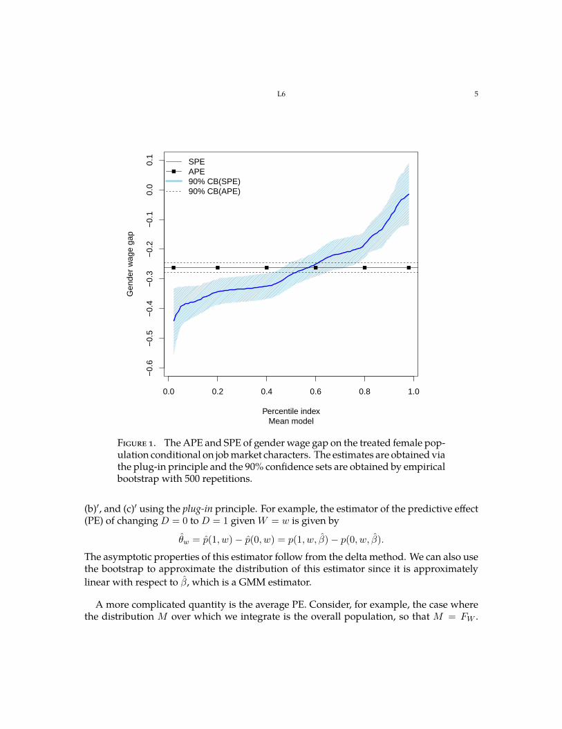
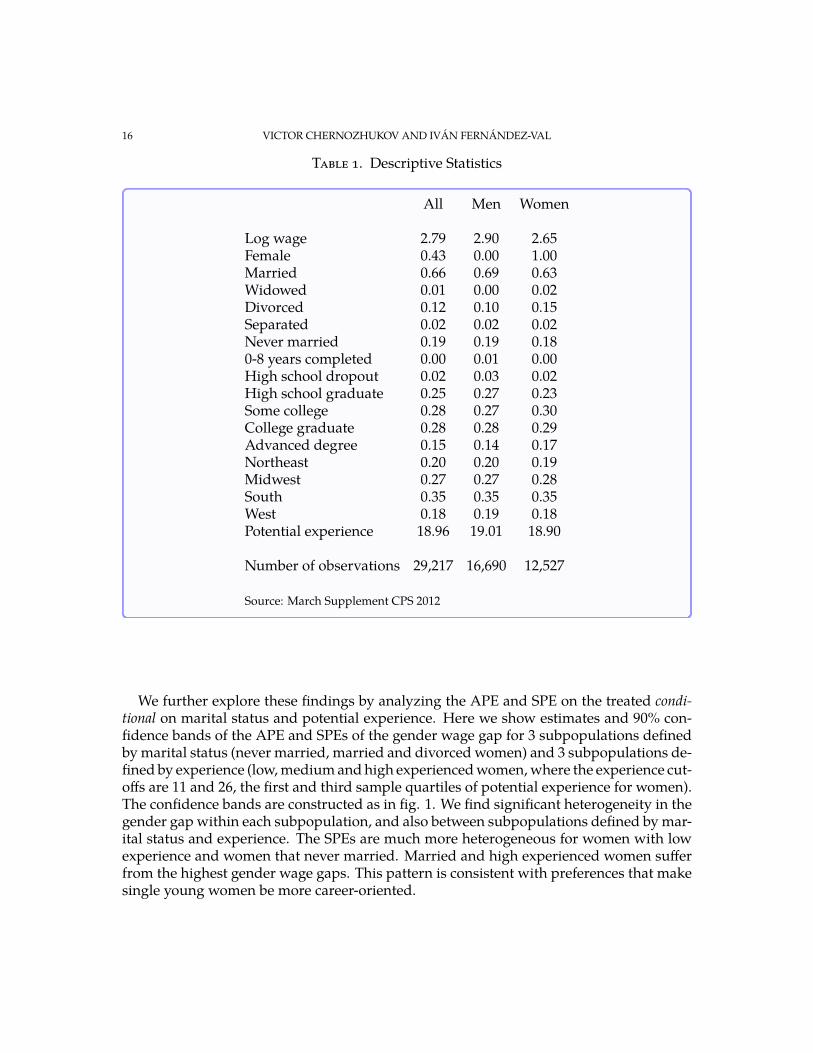

MIT OpenCourseWarehttpsocwmitedu
14382 EconometricsSpring 2017
For information about citing these materials or our Terms of Use visit httpsocwmiteduterms