IEEE TRANSACTIONS ON WIRELESS COMMUNICATIONS 1

Massive MIMO with Non-Ideal Arbitrary Arrays:Hardware Scaling Laws and Circuit-Aware Design

Emil Bjornson, Member, IEEE, Michail Matthaiou, Senior Member, IEEE, and Merouane Debbah, Fellow, IEEE

Abstract—Massive multiple-input multiple-output (MIMO)systems are cellular networks where the base stations (BSs) areequipped with unconventionally many antennas, deployed on co-located or distributed arrays. Huge spatial degrees-of-freedomare achieved by coherent processing over these massive arrays,which provide strong signal gains, resilience to imperfect channelknowledge, and low interference. This comes at the price of moreinfrastructure; the hardware cost and circuit power consumptionscale linearly/affinely with the number of BS antennas N . Hence,the key to cost-efficient deployment of large arrays is low-costantenna branches with low circuit power, in contrast to today’sconventional expensive and power-hungry BS antenna branches.Such low-cost transceivers are prone to hardware imperfections,but it has been conjectured that the huge degrees-of-freedomwould bring robustness to such imperfections. We prove thisclaim for a generalized uplink system with multiplicative phase-drifts, additive distortion noise, and noise amplification. Specifi-cally, we derive closed-form expressions for the user rates and ascaling law that shows how fast the hardware imperfections canincrease with N while maintaining high rates. The connectionbetween this scaling law and the power consumption of differenttransceiver circuits is rigorously exemplified. This reveals that onecan make the circuit power increase as

√N , instead of linearly,

by careful circuit-aware system design.

Index Terms—Achievable user rates, channel estimation, mas-sive MIMO, scaling laws, transceiver hardware imperfections.

I. INTRODUCTION

Interference coordination is the major limiting factor incellular networks, but modern multi-antenna base stations

c©2015 IEEE. Personal use of this material is permitted. Permission fromIEEE must be obtained for all other uses, in any current or future media,including reprinting/republishing this material for advertising or promotionalpurposes, creating new collective works, for resale or redistribution to serversor lists, or reuse of any copyrighted component of this work in other works.

Manuscript received July 4, 2014; revised November 3, 2014 and February16, 2015; accepted March 21, 2015. This research has received funding fromthe EU 7th Framework Programme under GA no ICT-619086 (MAMMOET).This research has been supported by ELLIIT, the International PostdocGrant 2012-228 from the Swedish Research Council and the ERC StartingGrant 305123 MORE (Advanced Mathematical Tools for Complex NetworkEngineering). The associate editor coordinating the review of this paper andapproving it for publication was G.Yue.

E. Bjornson was with the KTH Royal Institute of Technology, Stockholm,SE 100 44, Sweden, and with Supelec, Gif-sur-Yvette 91191, France. Heis now with the Department of Electrical Engineering (ISY), LinkopingUniversity, Linkoping, SE 581 83, Sweden (e-mail: emil.bjornson@liu.se).

M. Matthaiou is with the School of Electronics, Electrical Engineer-ing and Computer Science, Queen’s University Belfast, Belfast BT7 1NN,U.K., and also with the Department of Signals and Systems, ChalmersUniversity of Technology, Gothenburg, SE 412 96, Sweden (e-mail:m.matthaiou@qub.ac.uk).

M. Debbah is CentraleSupelec, Gif-sur-Yvette 91191, France (email: mer-ouane.debbah@centralesupelec.fr).

Digital Object Identifier 10.1109/TWC.2015.2420095

(BSs) can control the interference in the spatial domainby coordinated multipoint (CoMP) techniques [1]–[3]. Thecellular networks are continuously evolving to keep up withthe rapidly increasing demand for wireless connectivity [4].Massive densification, in terms of more service antennas perunit area, has been identified as a key to higher area throughputin future wireless networks [5]–[7]. The downside of densifi-cation is that even stricter requirements on the interference co-ordination need to be imposed. Densification can be achievedby adding more antennas to the macro BSs and/or distributingthe antennas by ultra-dense operator-deployment of smallBSs. These two approaches are non-conflicting and representthe two extremes of the massive MIMO paradigm [7]: alarge co-located antenna array or a geographically distributedarray (e.g., using a cloud RAN approach [8]). The massiveMIMO topology originates from [9] and has been given manyalternative names; for example, large-scale antenna systems(LSAS), very large MIMO, and large-scale multi-user MIMO.The main characteristics of massive MIMO are that each cellperforms coherent processing on an array of hundreds (or eventhousands) of active antennas, while simultaneously servingtens (or even hundreds) of users in the uplink and downlink.In other words, the number of antennas, N , and number ofusers per BS, K, are unconventionally large, but differ bya factor two, four, or even an order of magnitude. For thisreason, massive MIMO brings unprecedented spatial degrees-of-freedom, which enable strong signal gains from coherentreception/transmit beamforming, give nearly orthogonal userchannels, and resilience to imperfect channel knowledge [10].

Apart from achieving high area throughput, recent workshave investigated additional ways to capitalize on the hugedegrees-of-freedom offered by massive MIMO. Towards thisend, [5] showed that massive MIMO enables fully distributedcoordination between systems that operate in the same band.Moreover, it was shown in [11] and [12] that the transmituplink/downlink powers can be reduced as 1√

Nwith only a

minor loss in throughput. This allows for major reductionsin the emitted power, but is actually bad from an overallenergy efficiency (EE) perspective—the EE is maximized byincreasing the emitted power with N to compensate for theincreasing circuit power consumption [13].

This paper explores whether the huge degrees-of-freedomoffered by massive MIMO provide robustness to transceiverhardware imperfections/impairments; for example, phasenoise, non-linearities, quantization errors, noise amplification,and inter-carrier interference. Robustness to hardware imper-fections has been conjectured in overview articles, such as [7].Such a characteristic is notably important since the deployment

arX

iv:1

409.

0875

v3 [

cs.I

T]

29

Apr

201

5

IEEE TRANSACTIONS ON WIRELESS COMMUNICATIONS 2

cost and circuit power consumption of massive MIMO scaleslinearly with N , unless the hardware accuracy constraints canbe relaxed such that low-power, low-cost hardware is deployedwhich is more prone to imperfections. Constant envelopeprecoding was analyzed in [14] to facilitate the use of power-efficient amplifiers in the downlink, while the impact of phase-drifts was analyzed and simulated for single-carrier systemsin [15] and for orthogonal frequency-division multiplexing(OFDM) in [16]. A preliminary proof of the conjecture wasgiven in [17], but the authors therein considered only additivedistortions and, thus, ignored other important characteristicsof hardware imperfections. That paper showed that one cantolerate distortion variances that increase as

√N with only

minor throughput losses, but did not investigate what thisimplies for the design of different transceiver circuits.

In this paper, we consider a generalized uplink massiveMIMO system with arbitrary array configurations (e.g., co-located or distributed antennas). Based on the extensive liter-ature on modeling of transceiver hardware imperfections (see[3], [4], [15], [18]–[24] and references therein), we proposea tractable system model that jointly describes the impactof multiplicative phase-drifts, additive distortion noise, noiseamplification, and inter-carrier interference. This stands incontrast to the previous works [15]–[17], which each inves-tigated only one of these effects. The following are the maincontributions of this paper:

• We derive a new linear minimum mean square error(LMMSE) channel estimator that accounts for hardwareimperfections and allows the prediction of the detrimentalimpact of phase-drifts.

• We present a simple and general expression for theachievable uplink user rates and compute it in closed-form, when the receiver applies maximum ratio combin-ing (MRC) filters. We prove that the additive distortionnoise and noise amplification vanish asymptotically asN → ∞, while the phase-drifts remain but are notexacerbated.

• We obtain an intuitive scaling law that shows how fastwe can tolerate the levels of hardware imperfectionsto increase with N , while maintaining high user rates.This is an analytic proof of the conjecture that massiveMIMO systems can be deployed with inexpensive low-power hardware without sacrificing the expected majorperformance gains. The scaling law provides sufficientconditions that hold for any judicious receive filters.

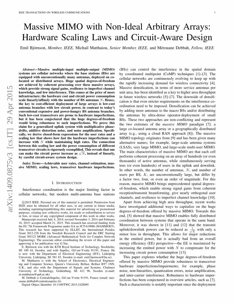
• The practical implications of the scaling law are exem-plified for the main circuits at the receiver, namely, theanalog-to-digital converter (ADC), low noise amplifier(LNA), and local oscillator (LO). The main componentsof a typical receiver are illustrated in Fig. 1. The scalinglaw reveals the tradeoff between hardware cost, level ofimperfections, and circuit power consumption. In partic-ular, it shows how a circuit-aware design can make thecircuit power consumption increase as

√N instead of N .

• The analytic results are validated numerically in a realis-tic simulation setup, where we consider different antennadeployment scenarios, common and separate LOs, dif-

DSP

Filter

Receiveantenna 1

ADCLNA Mixer

LO

Filter

Receiveantenna N

ADCLNA Mixer

LO

Fig. 1. Block diagram of a typical N -antenna receiver. The main circuitsare shown, but these can be complemented with additional intermediate filtersand amplifiers depending on the implementation. Most of the circuits affectonly one antenna, whilst the LO can be either common for all antennas ordifferent.

ferent pilot sequence designs, and two types of receivefilters. A key observation is that separate LOs can providebetter performance than a common LO, since the phase-drifts average out and the interference is reduced. This isalso rigorously supported by the analytic scaling law.

This paper extends substantially our conference papers [25]and [26], by generalizing the propagation model, generalizingthe analysis according to the new model, and providing morecomprehensive simulations. The paper is organized as follows:In Section II, the massive MIMO system model under consid-eration is presented. In Section III, a detailed performanceanalysis of the achievable uplink user rates is pursued and theimpact of hardware imperfections is characterized, while inSection IV we provide guidelines for circuit-aware design inorder to minimize the power dissipation of receiver circuits.Our theoretical analysis is corroborated with simulations inSection V, while Section VI concludes the paper.

Notation: The following notation is used throughout thepaper: Boldface (lower case) is used for column vectors, x,and (upper case) for matrices, X. Let XT, X∗, and XH

denote the transpose, conjugate, and conjugate transpose of X,respectively. A diagonal matrix with a1, . . . , aN on the maindiagonal is denoted as diag(a1, . . . , aN ), while IN is an N×Nidentity matrix. The set of complex-valued N × K matricesis denoted by CN×K . The expectation operator is denotedE· and , denotes definitions. The matrix trace function istr(·) and ⊗ is the Kronecker product. A Gaussian randomvariable x is denoted x ∼ N (x, q), where x is the mean andq is the variance. A circularly symmetric complex Gaussianrandom vector x is denoted x ∼ CN (x,Q), where x is themean and Q is the covariance matrix. The big O notationf(x) = O(g(x)) means that

∣∣∣ f(x)g(x)

∣∣∣ is bounded as x→∞.

II. SYSTEM MODEL WITH HARDWARE IMPERFECTIONS

We consider the uplink of a cellular network with L ≥ 1cells. Each cell consists of K single-antenna user equipments(UEs) that communicate simultaneously with an array of Nantennas, which can be either co-located at a macro BS ordistributed over multiple fully coordinated small BSs. Theanalysis of our paper holds for any N and K, but we

IEEE TRANSACTIONS ON WIRELESS COMMUNICATIONS 3

are primarily interested in massive MIMO topologies, whereN K 1. The frequency-flat channel from UE k in celll to BS j is denoted as hjlk ,

[h(1)jlk . . . h

(N)jlk

]T∈ CN×1

and is modeled as Rayleigh block fading. This means thatit has a static realization for a coherence block of T chan-nel uses and independent realizations between blocks.1 TheUEs’ channels are independent. Each realization is complexGaussian distributed with zero mean and covariance matrixΛjlk ∈ CN×N :

hjlk ∼ CN (0,Λjlk). (1)

The covariance matrix Λjlk , diag(λ(1)jlk, . . . , λ

(N)jlk

)is

assumed to be diagonal, which holds if the inter-antennadistances are sufficiently large and the multi-path scatteringenvironment is rich [27].2 The average channel attenuationλ(n)jlk is different for each combination of cells, UE index, and

receive antenna index n. It depends, for example, on the arraygeometry and the UE location. Even for co-located antennasone might have different values of λ(n)jlk over the array, becauseof the large aperture that may create variations in the shadowfading.

The received signal yj(t) ∈ CN×1 in cell j at a givenchannel use t ∈ 1, . . . , T in the coherence block is conven-tionally modeled as [9]–[12]

yj(t) =

L∑l=1

Hjlxl(t) + nj(t) (2)

where the transmit signal in cell l is xl(t) =[xl1(t) . . . xlK(t)]T ∈ CK×1 and we use the notationHjl = [hjl1 . . . hjlK ] ∈ CN×K for brevity. The scalar signalxlk(t) sent by UE k in cell l at channel use t is either adeterministic pilot symbol (used for channel estimation) or aninformation symbol from a Gaussian codebook; in any case,we assume that the expectation of the transmit energy persymbol is bounded as E|xlk(t)|2 ≤ plk. The thermal noisevector nj(t) ∼ CN (0, σ2IN ) is spatially and temporallyindependent and has variance σ2.

The conventional model in (2) is well-accepted for small-scale MIMO systems, but has an important drawback whenapplied to massive MIMO topologies: it assumes that the largeantenna array consists of N high-quality antenna brancheswhich are all perfectly synchronized. Consequently, the de-ployment cost and total power consumption of the circuitsattached to each antenna would at least grow linearly withN , thereby making the deployment of massive MIMO ratherquestionable, if not prohibitive, from an overall cost andefficiency perspective.

In this paper, we analyze the far more realistic scenarioof having inexpensive hardware-constrained massive MIMOarrays. More precisely, each receive array experiences hard-ware imperfections that distort the communication. The exact

1The size of the time/frequency block where the channels are static dependson UE mobility and propagation environment: T is the product of thecoherence time τc and coherence bandwidth Wc, thus τc = 5 ms andWc = 100 kHz gives T = 500.

2The analysis and main results of this paper can be easily extended toarbitrary non-diagonal covariance matrices as in [11] and [17], but at the costof complicating the notation and expressions.

distortion characteristics depend generally on which modula-tion scheme is used; for example, OFDM [18], filter bankmulticarrier (FBMC) [28], or single-carrier transmission [15].Nevertheless, the distortions can be classified into three dis-tinct categories: 1) received signals are shifted in phase; 2)distortion noise is added with a power proportional to the totalreceived signal power; and 3) thermal noise is amplified andchannel-independent interference is added. To draw generalconclusions on how these distortion categories affect massiveMIMO systems, we consider a generic system model withhardware imperfections. The received signal in cell j at a givenchannel use t ∈ 1, . . . , T is modeled as

yj(t) = Dφj(t)

L∑l=1

Hjlxl(t) + υj(t) + ηj(t) (3)

where the channel matrices Hjl and transmitted signals xl(t)are exactly as in (2). The hardware imperfections are definedas follows:

1) The matrix Dφj(t), diag

(eıφj1(t), . . . , eıφjN (t)

)de-

scribes multiplicative phase-drifts, where ı is the imag-inary unit. The variable φjn(t) is the phase-drift at thenth receive antenna in cell j at time t. Motivated by thestandard phase-noise models in LOs [21], φjn(t) followsa Wiener process

φjn(t) ∼ N (φjn(t− 1), δ) (4)

which equals the previous realization φjn(t − 1) plusan independent Gaussian innovation of variance δ. Thephase-drifts can be either independent or correlatedbetween the antennas; for example, co-located arraysmight have a common LO (CLO) for all antennaswhich makes the phase-drifts φjn(t) identical for alln = 1, . . . , N . In contrast, distributed arrays might haveseparate LOs (SLOs) at each antenna, which make thedrifts independent, though we let the variance δ be equalfor simplicity. Both cases are considered herein.

2) The distortion noise υj(t) ∼ CN (0,Υj(t)), where

Υj(t) , κ2L∑l=1

K∑k=1

E|xlk(t)|2diag

(|h(1)jlk|

2, . . . , |h(N)jlk |

2

)(5)

for given channel realizations, where the double-sumgives the received power at each antenna. Thus, thedistortion noise is independent between antennas andchannel uses, and the variance at a given antenna isproportional to the current received signal power at thisantenna. This model can describe the quantization noisein ADCs with gain control [19], approximate genericnon-linearities [4, Chapter 14], and approximate theleakage between subcarriers due to calibration errors.The parameter κ ≥ 0 describes how much weaker thedistortion noise magnitude is compared to the signalmagnitude.

3) The receiver noise ηj(t) ∼ CN (0, ξIN ) is independentof the UE channels, in contrast to the distortion noise.This term includes thermal noise, which typically isamplified by LNAs and mixers in the receiver hardware,

IEEE TRANSACTIONS ON WIRELESS COMMUNICATIONS 4

and interference leakage from other frequency bandsand/or other networks. The receiver noise variance mustsatisfy ξ ≥ σ2. If there is no interference leakage,F = ξ

σ2 is called the noise amplification factor.

This tractable generic model of hardware imperfections atthe BSs is inspired by a plethora of prior works [3], [4],[15], [18]–[24] and characterizes the joint behavior of allhardware imperfections at the BSs—these can be uncalibratedimperfections or residual errors after calibration. The modelin (3) is characterized by three parameters: δ, κ, and ξ. Themodel is compatible with the conventional model in (2), whichis obtained by setting ξ = σ2 and δ=κ= 0. The analysis inthis paper holds for arbitrary parameter values. Section IVexemplifies the connection between imperfections in the maintransceiver circuits of the BSs and the three parameters. Theseconnections allow for circuit-aware design of massive MIMOsystems.

In the next section, we derive a channel estimator andachievable UE rates for the system model in (3). By analyzingthe performance as N → ∞, we bring new insights into thefundamental impact of hardware imperfections (in particular,in terms of δ, κ, and ξ).

III. PERFORMANCE ANALYSIS

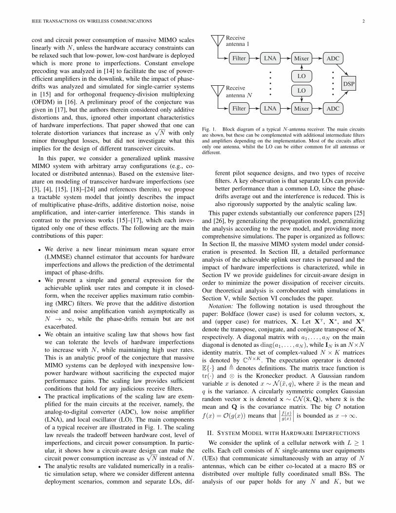
In this section, we derive achievable UE rates for the uplinkmulti-cell system in (3) and analyze how these depend onthe number of antennas and hardware imperfections. We firstneed to specify the transmission protocol.3 The T channeluses of each coherence block are split between transmission ofuplink pilot symbols and uplink data symbols. It is necessaryto dedicate B ≥ K channel uses for pilot transmission ifthe receiving array should be able to spatially separate thedifferent UEs in the cell. The remaining T − B channeluses are allocated for data transmission. The pilot symbolscan be distributed in different ways: for example, placed inthe beginning of the block [17], in the middle of the block[29], uniformly distributed as in the LTE standard [30], or acombination of these approaches [22]. These different casesare illustrated in Fig. 2. The time indices used for pilottransmission are denoted by τ1, . . . , τB ∈ 1, . . . , T, whileD , 1, . . . , T \ τ1, . . . , τB are the time indices for datatransmission.

A. Channel Estimation under Hardware Imperfections

Based on the transmission protocol, the pilot sequence ofUE k in cell j is xjk , [xjk(τ1) . . . xjk(τB)]T ∈ CB×1. Thepilot sequences are predefined and can be selected arbitrarilyunder the power constraints. Our analysis supports any choice,but it is reasonable to make xj1, . . . , xjK in cell j mutuallyorthogonal to avoid intra-cell interference (this is the reasonto have B ≥ K).

3We assume that the same protocol is used in all cells, for analyticsimplicity. It was shown in [12, Remark 5] that nothing substantially differentwill happen if this assumption is relaxed.

Pilot sequence Data symbols

Pilot sequenceData symbols

(a)

(b)

(c)

(d)

Coherence block

Data symbols

Fig. 2. Examples of different ways to distribute the B pilot symbols over thecoherence block of length T : (a) beginning of block; (b) middle of block; (c)uniform pilot distribution; (d) preamble and a few distributed pilot symbols.

Example 1: Let Xj , [xj1 . . . xjK ] denote the pilot se-quences in cell j. The simplest example of linearly indepen-dent pilot sequences (with B = K) is

Xtemporalj , diag(

√pj1, . . . ,

√pjK) (6)

where the different sequences are temporally orthogonal sinceonly UE k transmits at time τk. Alternatively, the pilotsequences can be made spatially orthogonal so that all UEstransmit at every pilot transmission time, which effectivelyincreases the total pilot energy by a factor K. The canonicalexample is to use a scaled discrete Fourier transform (DFT)matrix [31]:

Xspatialj ,

1 1 . . . 1

1 WK . . . WK−1K

......

......

1 WB−1K . . . W

(B−1)(K−1)K

Xtemporalj (7)

where WK , e−ı2π/K .The pilot sequences can also be jointly designed across

cells, to reduce inter-cell interference during pilot transmis-sion. Since network-wide pilot orthogonality requires B ≥LK, which typically is much larger than the coherence blocklength T , practical networks need to balance between pilotorthogonality and inter-cell interference. A key design goal isto allocate non-orthogonal pilot sequences to UEs that havenearly orthogonal channel covariance matrices; for example,by making tr(ΛjjkΛjlm) small for any combination of a UEk in cell j and a UE m in cell l, as suggested in [32].

For any given set of pilot sequences, we now derive esti-mators of the effective channels

hjlk(t) , Dφj(t)hjlk (8)

at any channel use t ∈ 1, . . . , T and for all j, l, k. Theconventional multi-antenna channel estimators from [33]–[35]cannot be applied in this paper since the generalized systemmodel in (3) has two non-standard properties: the pilot trans-mission is corrupted by random phase-drifts and the distortionnoise is statistically dependent on the channels. Therefore, wederive a new LMMSE estimator for the system model at hand.

Theorem 1: Let ψj ,[yTj (τ1) . . . yT

j (τB)]T ∈ CBN

denote the combined received signal in cell j from the pilottransmission. The LMMSE estimate of hjlk(t) at any channel

IEEE TRANSACTIONS ON WIRELESS COMMUNICATIONS 5

SINRjk(t) =pjk|EvH

jk(t)hjjk(t)|2L∑l=1

K∑m=1

plmE|vH

jk(t)hjlm(t)|2 − pjk|EvH

jk(t)hjjk(t)|2 + E|vH

jk(t)υj(t)|2+ ξE‖vjk(t)‖2(20)

use t ∈ 1, . . . , T for any l and k is

hjlk(t) =(xH

lkDδ(t) ⊗Λjlk

)Ψ−1j ψj (9)

where

Dδ(t) , diag

(e−

δ2 |t−τ1|, . . . , e−

δ2 |t−τB |

), (10)

Ψj ,L∑`=1

K∑m=1

X`m ⊗Λj`m + ξIBN , (11)

X`m , X`m + κ2D|x`m|2 , (12)

D|x`m|2 , diag

(|x`m(τ1)|2, . . . , |x`m(τB)|2

), (13)

while the element (b1, b2) of X`m ∈ CB×B is

[X`m]b1,b2 =

|x`m(τb1)|2, b1 = b2,

x`m(τb1)x∗`m(τb2)e−δ2 |τb1−τb2 |, b1 6= b2.

(14)The corresponding error covariance matrix is

Cjlk(t) = E(

hjlk(t)− hjlk(t))(

hjlk(t)− hjlk(t))H

= Λjlk −(xH

lkDδ(t) ⊗Λjlk

)Ψ−1j (DH

δ(t)xlk ⊗Λjlk)

(15)

and the mean-squared error (MSE) is MSEjlk(t) =tr(Cjlk(t)).

Proof: The proof is given in Appendix B.It is important to note that although the channels are block

fading, the phase-drifts caused by hardware imperfectionsmake the effective channels hjlk(t) change between everychannel use. The new LMMSE estimator in Theorem 1 pro-vides different estimates for each time index t ∈ D used fordata transmission—this is a prediction, interpolation, or retro-spection depending on how the pilot symbols are distributed inthe coherence block (recall Fig. 2). The LMMSE estimator isthe same for systems with independent and correlated phase-drifts which brings robustness to modeling errors, but alsomeans that there exist better non-linear estimators that canexploit phase-drift correlations, though we do not pursue thisissue further in this paper.

The estimator expression is simplified in the special case ofco-located arrays, as shown by the following corollary.

Corollary 1: If Λjlk = λjlkIN for all j, l, and k, theLMMSE estimate in (9) simplifies to

hjlk(t) =

(λjlkx

H

lkDδ(t)Ω−1j ⊗ IN

)ψj (16)

and the error covariance matrix in (15) becomes

Cjlk(t) = λjlk

(1− λjlkxH

lkDδ(t)Ω−1j DH

δ(t)xlk

)IN (17)

where Ωj is the Hermitian matrix

Ωj ,L∑`=1

K∑m=1

λj`mX`m + ξIB . (18)

Next, we use these channel estimates to design receive filtersand derive achievable UE rates.

B. Achievable UE Rates under Hardware Imperfections

It is difficult to compute the maximum achievable UE rateswhen the receiver has imperfect channel knowledge [36], andhardware imperfections are not simplifying this task. Upperbounds on the achievable rates were obtained in [17] and[37]. In this paper, we want to guarantee certain performanceand thus seek simple achievable (but suboptimal) rates. Thefollowing lemma provides such rate expressions and buildsupon well-known techniques from [9], [15], [36], [38], [39]for computing lower bounds on the mutual information.

Lemma 1: Suppose the receiver in cell j has completestatistical channel knowledge and applies the linear receivefilters vH

jk(t) ∈ C1×N , for t ∈ D, to detect the signal from itskth UE. An ergodic achievable rate for this UE is

Rjk =1

T

∑t∈D

log2

(1 + SINRjk(t)

)[bit/channel use] (19)

where SINRjk(t) is given in (20) at the top of this page andall UEs use full power (i.e., E|xlk(t)|2 = plk for all l, k).

Proof: The proof is given in Appendix C.The achievable UE rates in Lemma 1 can be computed for

any choice of receive filters, using numerical methods; theMMSE receive filter is simulated in Section V. Note that thesum in (19) has |D| = T −B terms, while the pre-log factor1T also accounts for the B channel uses of pilot transmissions.The next theorem gives new closed-form expressions for allthe expectations in (20) when using MRC receive filters.

Theorem 2: The expectations in the SINR expression (20)are given in closed form by (21)–(24), at the top of the nextpage, when the MRC receive filter vMRC

jk (t) = hjjk(t) is usedin cell j. The nth column of IN is denoted by en ∈ CN×1 inthis paper.

Proof: The proof is given in Appendix D.By substituting the expressions from Theorem 2 into (20),

we obtain closed-form UE rates that are achievable usingMRC filters. Although the expressions in (21)–(24) are easyto compute, their interpretation is non-trivial. The size of eachterm depends on the setup and scales differently with N ; notethat each trace-expression and/or sum over the antennas givea scaling factor of N . This property is easily observed in thespecial case of co-located antennas:

Corollary 2: If Λjlk = λjlkIN for all j, l, and k, the MRCreceive filter yields:

IEEE TRANSACTIONS ON WIRELESS COMMUNICATIONS 6

E‖vjk(t)‖2 = tr((

xH

jkDδ(t) ⊗Λjjk

)Ψ−1j

(DH

δ(t)xjk ⊗Λjjk

))(21)

EvH

jk(t)hjjk(t) = E‖vjk(t)‖2 (22)

E|vH

jk(t)hjlm(t)|2 = tr(Λjlm

(xH

jkDδ(t) ⊗Λjjk

)Ψ−1j

(DH

δ(t)xjk ⊗Λjjk

))(23)

+

N∑

n1=1

N∑n2=1

λ(n1)jjk λ

(n1)jlm λ

(n2)jjk λ

(n2)jlm

(xH

jkDδ(t) ⊗ eHn1

)Ψ−1j

(Xlm ⊗ en1

eHn2

)Ψ−1j

(DH

δ(t)xjk ⊗ en2

)if a CLO(

tr((

xH

jkDδ(t) ⊗Λjjk

)Ψ−1j

(DH

δ(t)xlm ⊗Λjlm

)))2if SLOs

+

N∑n=1

(λ(n)jjkλ

(n)jlm

)2 (xH

jkDδ(t) ⊗ eHn

)Ψ−1j

(κ2D|xlm|2 ⊗ eneH

n

)Ψ−1j

(DH

δ(t)xjk ⊗ en

)if a CLO

N∑n=1

(λ(n)jjkλ

(n)jlm

)2 (xH

jkDδ(t) ⊗ eHn

)Ψ−1j

((Xlm −DH

δ(t)xlmxH

lmDδ(t))⊗ eneHn

)Ψ−1j

(DH

δ(t)xjk ⊗ en

)if SLOs

E|vH

jk(t)υj(t)|2 = κ2L∑l=1

K∑m=1

plmtr(Λjlm

(xH

jkDδ(t) ⊗Λjjk

)Ψ−1j

(DH

δ(t)xjk ⊗Λjjk

))(24)

+ κ2L∑l=1

K∑m=1

N∑n=1

plm

(λ(n)jjkλ

(n)jlm

)2 (xH

jkDδ(t) ⊗ eH

n

)Ψ−1j (Xlm ⊗ eneH

n)Ψ−1j

(DH

δ(t)xjk ⊗ en

)

E‖vjk(t)‖2 = Nλ2jjkxH

jkDδ(t)Ω−1j DH

δ(t)xjk

EvH

jk(t)hjjk(t) = E‖vjk(t)‖2E|vH

jk(t)hjlm(t)|2 = λjlmE‖vjk(t)‖2+Nλ2jjkλ

2jlmxH

jkDδ(t)Ω−1j XlmΩ−1j DH

δ(t)xjk +N(N−1)

×

λ2jjkλ

2jlmxH

jkDδ(t)Ω−1j XlmΩ−1j DH

δ(t)xjk if a CLOλ2jjkλ

2jlm|xH

jkDδ(t)Ω−1j DH

δ(t)xlm|2 if SLOs

E|vH

jk(t)υj(t)|2 = κ2E‖vjk(t)‖2L∑l=1

K∑m=1

plmλjlm

+κ2L∑l=1

K∑m=1

plmNλ2jjkλ

2jlmxH

jkDδ(t)Ω−1j XlmΩ−1j DH

δ(t)xjk.

As seen from this corollary, most terms scale linearly withN but there are a few terms that scale as N2. The latter termsdominate in the asymptotic analysis below.

The difference between having a CLO and SLOsonly manifests itself in the second-order momentsE|vH

jk(t)hjlm(t)|2. Hence, the desired signal qualityis the same in both cases, while the interference terms aredifferent; the case with the smallest interference variance∑Ll=1

∑Km=1 plmE|vH

jk(t)hjlm(t)|2 gives the largest ratefor UE k in cell j. These second-order moments dependon the pilot sequences, channel covariance matrices, andphase-drifts. By looking at (23) in Theorem 2 (or thecorresponding expression in Corollary 2), we see that theonly difference is that two occurrences of X`m in the caseof a CLO are replaced by DH

δ(t)x`mxH

`mDδ(t) in the case ofSLOs. These terms are equal when there are no phase-drifts(i.e., δ = 0), while the difference grows larger with δ. Inparticular, the term X`m is unaffected by the time index t,while the corresponding terms for SLOs decay as e−δt (fromDδ(t)). The following example provides the intuition behindthis result.

Example 2: The interference power in (20) consists ofmultiple terms of the form E|vH

jk(t)Dφj(t)hjlm|2. Suppose

that the receive filter is set to some constant vjk(t) =vjk. If a CLO is used, we have E|vH

jkDφj(t)hjlm|2 =

E|vH

jkhjlm|2, which is independent of the phase-drifts sinceall elements of vjk are rotated in the same way. In con-trast, each component of vjk is rotated in an independentrandom manner with SLOs, which reduces the average in-terference power since the components of the inner productvH

jkDφj(t)hjlm add up incoherently. Consequently, the re-

ceived interference power is reduced by SLOs while it remainsthe same with a CLO.

To summarize, we expect SLOs to provide larger UE ratesthan a CLO, because the interference reduces with t whenthe phase-drifts are independent, at the expense of increasingthe deployment cost by having N LOs. This observation isvalidated by simulations in Section V.

C. Asymptotic Analysis and Hardware Scaling LawsThe closed-form expressions in Theorem 2 and Corollary

2 can be applied to cellular networks of arbitrary (finite)dimensions. In massive MIMO, the asymptotic behavior oflarge antenna arrays is of particular interest. In this section, weassume that the N receive antennas in each cell are distributedover A ≥ 1 spatially separated subarrays, where each subarraycontains N

A antennas. This assumption is made for analytictractability, but also makes sense in many practical scenarios.Each subarray is assumed to have an inter-antenna distancemuch smaller than the propagation distances to the UEs, suchthat λ(a)jlk is the average channel attenuation to all antennas insubarray a in cell j from UE k in cell l. Hence, the channelcovariance matrix Λjlk ∈ CN×N can be factorized as

Λjlk = diag

(λ(1)jlk, . . . , λ

(A)jlk

)︸ ︷︷ ︸

,Λ(A)jlk ∈CA×A

⊗INA. (25)

IEEE TRANSACTIONS ON WIRELESS COMMUNICATIONS 7

By letting the number of antennas in each subarray grow large,we obtain the following property.

Corollary 3: If the MRC receive filter is used and thechannel covariance matrices can be factorized as in (25), then

SINRjk(t) =pjkSigjk

L∑l=1

K∑m=1

plmIntjklm − pjkSigjk+O(

1N

) (26)

where the signal part is

Sigjk =(

tr((

xH

jkDδ(t)⊗Λ(A)jjk

)Ψ−1j

(Dδ(t)xjk⊗Λ

(A)jjk

)))2(27)

the interference terms with a CLO are

IntCLOjklm =

A∑a1=1

A∑a2=1

λ(a1)jjk λ

(a1)jlm λ

(a2)jjk λ

(a2)jlm

(xH

jkDδ(t)⊗eH

a1

)× Ψ

−1j

(Xlm ⊗ ea1e

H

a2

)Ψ−1j

(DH

δ(t)xjk⊗ea2

)(28)

and the interference terms with SLOs are

IntSLOsjklm =

(tr((

xH

jkDδ(t)⊗Λ(A)jjk

)Ψ−1j

(DH

δ(t)xlm⊗Λ(A)jlm

)))2.

(29)

In these expresssions Ψj ,∑L`=1

∑Km=1 X`m⊗Λ

(A)j`m+ξIAB ,

ea is the ath column of IA, and the big O notation O( 1N )

denotes terms that go to zero as 1N or faster when N →∞.

Proof: The proof is given in Appendix E.This corollary shows that the distortion noise and receiver

noise vanish as N → ∞. The phase-drifts remain, buthave no dramatic impact since these affect the numeratorand denominator of the asymptotic SINR in (26) in similarways. The simulations in Section V show that the phase-driftdegradations are not exacerbated in massive MIMO systemswith SLOs, while the performance with a CLO improves withN but at a slower pace due to the phase-drifts.

The asymptotic SINRs are finite because both the signalpower and parts of the inter-cell and intra-cell interferencegrow quadratically with N . This interference scaling behavioris due to so-called pilot contamination (PC) [9], [40], whichrepresents the fact that a BS cannot fully separate signals fromUEs that interfered with each other during pilot transmission.4

Intra-cell PC is, conventionally, avoided by making the pilotsequences orthogonal in space; for example, by using theDFT pilot matrix Xspatial

j in Example 1. Unfortunately, thephase-drifts break any spatial pilot orthogonality. Hence, it isreasonable to remove intra-cell PC by assigning temporallyorthogonal sequences, such as Xtemporal

j in Example 1. Notethat with temporal orthogonality the total pilot energy per UE,‖xjk‖2, is reduced by 1

K since the energy per pilot symbol isconstrained. Consequently, the simulations in Section V revealthat temporally orthogonal pilot sequences are only beneficialfor extremely large arrays. Inter-cell PC cannot generally beremoved, because there are only B ≤ T orthogonal sequencesin the whole network, but it can be mitigated by allocatingthe same pilot to UEs that are well separated (e.g., in terms

4Pilot contamination can be mitigated through semi-blind channel estima-tion as proposed in [41], but the UE rates will still be limited by hardwareimperfections [17].

of second-order channel statistics such as different path-lossesand spatial correlation [32]).

Apparently, the detrimental impact of hardware imperfec-tions vanishes almost completely as N grows large. This resultholds for any fixed values of the parameters δ, κ, and ξ. Infact, the hardware imperfections may even vanish when thehardware quality is gradually decreased with N . The nextcorollary formulates analytically such an important hardwarescaling law.

Corollary 4: Suppose the hardware imperfection param-eters are replaced as κ2 7→ κ20N

z1 , ξ 7→ ξ0Nz2 , and

δ 7→ δ0(1 + loge(Nz3)), for some given scaling exponents

z1, z2, z3 ≥ 0 and some initial values κ0, ξ0, δ0 ≥ 0. Moreover,let all pilot symbols be non-zero: xjk(τb) > 0 for all j, k,and b. Then, all the SINRs, SINRjk(t), under MRC receivefiltering converge to non-zero limits as N →∞ ifmax(z1, z2) ≤ 1

2 and z3 = 0 for a CLOmax(z1, z2) + z3 min

τ∈τ1,...,τBδ0|t−τ |

2 ≤ 12 for SLOs.

(30)Proof: The proof is given in Appendix F.

This corollary proves that we can tolerate stronger hardwareimperfections as the number of antennas increases. This isa very important result for practical deployments, becausewe can relax the design constraints on the hardware qualityas N increases. In particular, we can achieve better energyefficiency in the circuits and/or lower hardware costs byaccepting larger distortions than conventionally. This propertyhas been conjectured in overview articles, such as [7], andwas proved in [17] using a simplified system model with onlyadditive distortion noise. Corollary 4 shows explicitly that theconjecture is also true for multiplicative phase-drifts, receivernoise, and inter-carrier interference. Going a step further,Section IV exemplifies how the scaling law may impact thecircuit design in practical deployments.

Since Corollary 4 is derived for MRC filtering, (30) pro-vides a sufficient scaling condition also for any receive filterthat performs better than MRC. The scaling law for SLOsconsists of two terms: max(z1, z2) and z3 min

τ∈τ1,...,τBδ0|t−τ |

2 .

The first term max(z1, z2) shows that the additive distortionnoise and receiver noise can be increased simultaneously andindependently (as fast as

√N ), while the sum of the two terms

manifests a tradeoff between allowing hardware imperfectionsthat cause additive and multiplicative distortions. The scalinglaw for a CLO allows only for increasing the additive distor-tion noise and receiver noise, while the phase-drift varianceshould not be increased because only the signal gain (and notthe interference) is reduced by phase-drifts in this case; seeExample 2. Clearly, the system is particularly vulnerable tophase-drifts due to their accumulation and since they affectthe signal itself; even in the case of SLOs, the second termof (30) increases with T and the variance δ can scale onlylogarithmically with N . Note that we can accept larger phase-drift variances if the coherence block T is small and the pilotsymbols are distributed over the coherence block, which is inline with the results in [15].

IEEE TRANSACTIONS ON WIRELESS COMMUNICATIONS 8

IV. UTILIZING THE SCALING LAW:CIRCUIT-AWARE DESIGN

The generic system model with hardware imperfections in(3) describes a flat-fading multi-cell channel. This channel candescribe either single-carrier transmission over the full avail-able flat-fading bandwidth as in [22] or one of the subcarriersin a system based on multi-carrier modulation; for example,OFDM or FBMC as in [18], [28]. To some extent, it can alsodescribe single-carrier transmission over frequency-selectivechannels as in [15]. The mapping between the imperfections ina certain circuit in the receiving array to the three categories ofdistortions (defined in Section II) depends on the modulationscheme. For example, the multiplicative distortions caused byphase-noise leads also to inter-carrier interference in OFDMwhich is an additive noise-like distortion.

In this section, we exemplify what the scaling law inCorollary 4 means for the circuits depicted in Fig. 1. Inparticular, we show that the scaling law can be utilizedfor circuit-aware system design, where the cost and powerdissipation per circuit will be gradually decreased to achievea sub-linear cost/power scaling with the number of antennas.For clarity of presentation, we concentrate on single-carriertransmission over flat-fading channels, but mention briefly ifthe interpretation might change for multi-carrier modulation.

A. Analog-to-Digital Converter (ADC)

The ADC quantizes the received signal to a b bit resolution.Suppose the received signal power is Psignal and that auto-matic gain control is used to achieve maximum quantizationaccuracy irrespective of the received signal power. In terms ofthe originally received signal power Psignal, the quantizationin single-carrier transmission can be modeled as reducing thesignal power to (1 − 2−2b)Psignal and adding uncorrelatedquantization noise with power 2−2bPsignal [19, Eq. (17)]. Thismodel is particularly accurate for high ADC resolutions. Wecan include the quantization noise in the channel model (3)by normalizing the useful signal. The quantization noise isincluded in the additive distortion noise υj(t) and contributesto κ2 with 2−2b

1−2−2b , while the receiver noise variance ξ is scaledby a factor 1

1−2−2b due to the normalization. The scaling lawin Corollary 4 allows us to increase the variance κ2 as Nz1 forz1 ≤ 1

2 . This corresponds to reducing the ADC resolution byaround z1

2 log2(N) bits, which reduces cost and complexity.For example, we can reduce the ADC resolution per antennaby 2 bits if we deploy 256 antennas instead of one. For verylarge arrays, it is even sufficient to use 1-bit ADCs (cf. [42]).

The power dissipation of an ADC, PADC, is proportional to22b [19, Eq. (14)] and can, thus, be decreased approximatelyas 1/Nz1 . If each antenna has a separate ADC, the totalpower NPADC increases with N but proportionally to N1−z1 ,for z1 ≤ 1

2 , instead of N , due to the gradually lower ADCresolution. The scaling can thus be made as small as

√N .

B. Low Noise Amplifier (LNA)

The LNA is an analog circuit that amplifies the receivedsignal. It is shown in [43] that the behavior of an LNA is

characterized by the figure-of-merit (FoM) expression

FoMLNA =G

(F − 1)PLNA(31)

where F ≥ 1 is the noise amplification factor, G is theamplifier gain, and PLNA is the power dissipation in theLNA. Using this notation, the LNA contributes to the receivernoise variance ξ with Fσ2. For optimized LNAs, FoMLNA isa constant determined by the circuit architecture [43]; thus,FoMLNA basically scales with the hardware cost. The scalinglaw in Corollary 4 allows us to increase ξ as Nz2 for z2 ≤ 1

2 .The noise figure, defined as 10 log10(F ), can thus be increasedby z210 log10(N) dB. For example, at z2 = 1

2 we can allowan increase by 10 dB if we deploy 100 antennas instead ofone.

For a given circuit architecture, the invariance of theFoMLNA in (31) implies that we can decrease the powerdissipation (roughly) proportional to 1/Nz2 . Hence, we canmake the total power dissipation of the N LNAs, NPLNA,increase as N1−z2 instead of N by tolerating higher noiseamplification. The scaling can thus be made as small as

√N .

C. Local Oscillator (LO)

Phase noise in the LOs is the main source of multiplicativephase-drifts and changes the phases gradually at each channeluse. The average amount of phase-drifts that occurs under acoherence block is δT and depends on the phase-drift varianceδ and the block length T . If the LOs are free-running, the phasenoise is commonly modeled by the Wiener process (randomwalk) defined in Section II [15], [21]–[23], [44] and the phasenoise variance is given by

δ = 4π2f2c Tsζ (32)

where fc is the carrier frequency, Ts is the symbol time, andζ is a constant that characterizes the quality of the LO [21]. Ifδ and/or T are small, such that δT ≈ 0, the channel variationsdominate over the phase noise. However, phase noise canplay an important role when modeling channels with largecoherence time (e.g., fixed indoor users, line-of-sight, etc.) andas the carrier frequency increases (since δ = O(f2c ) while theDoppler spread reduces T as O(f−1c ) [22]. Relevant examplesare mobile broadband access to homes and WiFi at millimeterfrequencies.

The power dissipation PLO of the LO is coupled to ζ,such that PLOζ ≈ FoMLO where the FoM value FoMLO

depends on the circuit architecture [21], [45] and naturallyon the hardware cost. For a given architecture, we can allowlarger δ and, thereby, decrease the power PLO. The scalinglaw in Corollary 4 allows us to increase δ as (1 + loge(N

z3))when using SLOs. The power dissipation per LO can then bereduced as 1

1+z3 loge(N) . This reduction is only logarithmicin N , which stands in contrast to the 1/

√N scalings for

ADCs and LNAs (achieved by z1 = z2 = 12 ). Since linear

increase is much faster than logarithmic decay, the total powerNPLO with SLOs increases almost linearly with N ; thus, thebenefit is mostly cost and design related. In contrast, the phasenoise variance cannot be scaled when having a CLO, because

IEEE TRANSACTIONS ON WIRELESS COMMUNICATIONS 9

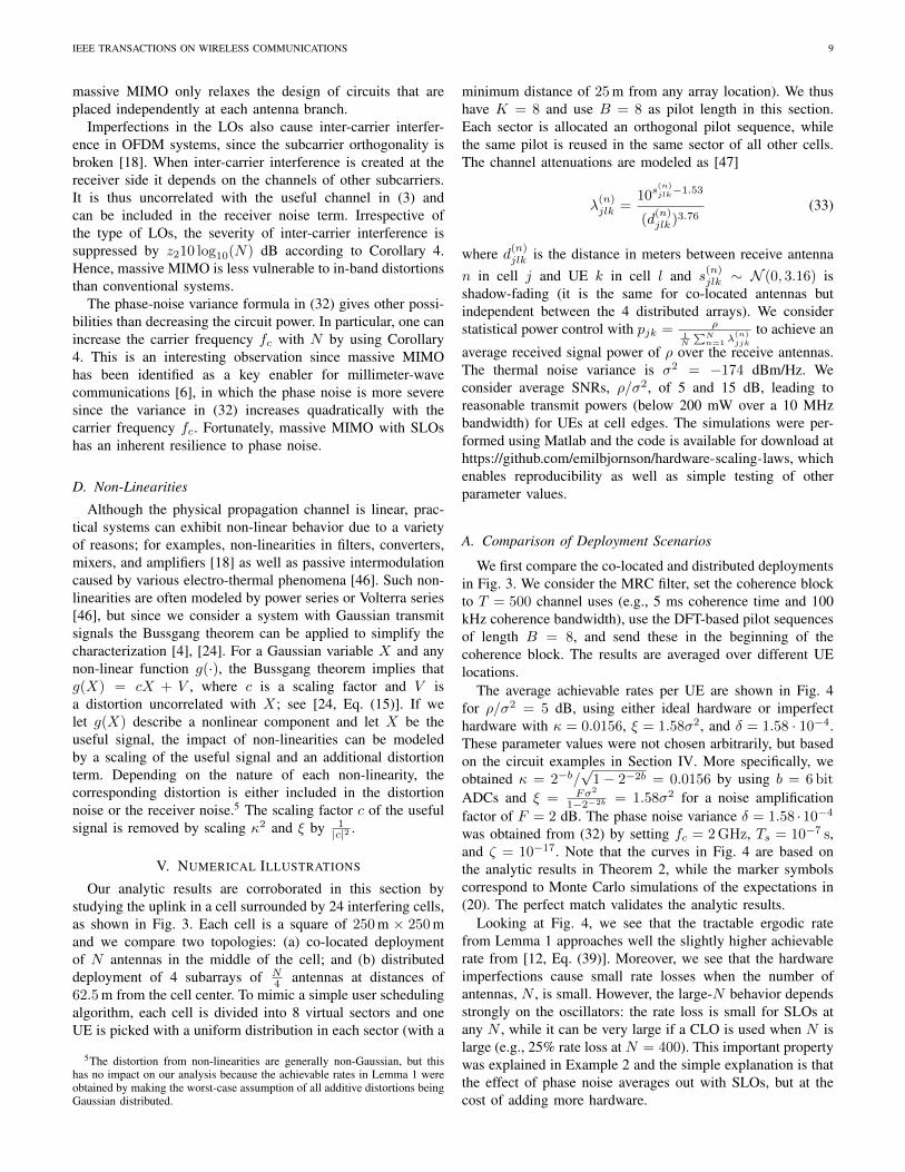
massive MIMO only relaxes the design of circuits that areplaced independently at each antenna branch.

Imperfections in the LOs also cause inter-carrier interfer-ence in OFDM systems, since the subcarrier orthogonality isbroken [18]. When inter-carrier interference is created at thereceiver side it depends on the channels of other subcarriers.It is thus uncorrelated with the useful channel in (3) andcan be included in the receiver noise term. Irrespective ofthe type of LOs, the severity of inter-carrier interference issuppressed by z210 log10(N) dB according to Corollary 4.Hence, massive MIMO is less vulnerable to in-band distortionsthan conventional systems.

The phase-noise variance formula in (32) gives other possi-bilities than decreasing the circuit power. In particular, one canincrease the carrier frequency fc with N by using Corollary4. This is an interesting observation since massive MIMOhas been identified as a key enabler for millimeter-wavecommunications [6], in which the phase noise is more severesince the variance in (32) increases quadratically with thecarrier frequency fc. Fortunately, massive MIMO with SLOshas an inherent resilience to phase noise.

D. Non-Linearities

Although the physical propagation channel is linear, prac-tical systems can exhibit non-linear behavior due to a varietyof reasons; for examples, non-linearities in filters, converters,mixers, and amplifiers [18] as well as passive intermodulationcaused by various electro-thermal phenomena [46]. Such non-linearities are often modeled by power series or Volterra series[46], but since we consider a system with Gaussian transmitsignals the Bussgang theorem can be applied to simplify thecharacterization [4], [24]. For a Gaussian variable X and anynon-linear function g(·), the Bussgang theorem implies thatg(X) = cX + V , where c is a scaling factor and V isa distortion uncorrelated with X; see [24, Eq. (15)]. If welet g(X) describe a nonlinear component and let X be theuseful signal, the impact of non-linearities can be modeledby a scaling of the useful signal and an additional distortionterm. Depending on the nature of each non-linearity, thecorresponding distortion is either included in the distortionnoise or the receiver noise.5 The scaling factor c of the usefulsignal is removed by scaling κ2 and ξ by 1

|c|2 .

V. NUMERICAL ILLUSTRATIONS

Our analytic results are corroborated in this section bystudying the uplink in a cell surrounded by 24 interfering cells,as shown in Fig. 3. Each cell is a square of 250 m × 250 mand we compare two topologies: (a) co-located deploymentof N antennas in the middle of the cell; and (b) distributeddeployment of 4 subarrays of N

4 antennas at distances of62.5 m from the cell center. To mimic a simple user schedulingalgorithm, each cell is divided into 8 virtual sectors and oneUE is picked with a uniform distribution in each sector (with a

5The distortion from non-linearities are generally non-Gaussian, but thishas no impact on our analysis because the achievable rates in Lemma 1 wereobtained by making the worst-case assumption of all additive distortions beingGaussian distributed.

minimum distance of 25 m from any array location). We thushave K = 8 and use B = 8 as pilot length in this section.Each sector is allocated an orthogonal pilot sequence, whilethe same pilot is reused in the same sector of all other cells.The channel attenuations are modeled as [47]

λ(n)jlk =

10s(n)jlk−1.53

(d(n)jlk)3.76

(33)

where d(n)jlk is the distance in meters between receive antennan in cell j and UE k in cell l and s

(n)jlk ∼ N (0, 3.16) is

shadow-fading (it is the same for co-located antennas butindependent between the 4 distributed arrays). We considerstatistical power control with pjk = ρ

1N

∑Nn=1 λ

(n)jjk

to achieve an

average received signal power of ρ over the receive antennas.The thermal noise variance is σ2 = −174 dBm/Hz. Weconsider average SNRs, ρ/σ2, of 5 and 15 dB, leading toreasonable transmit powers (below 200 mW over a 10 MHzbandwidth) for UEs at cell edges. The simulations were per-formed using Matlab and the code is available for download athttps://github.com/emilbjornson/hardware-scaling-laws, whichenables reproducibility as well as simple testing of otherparameter values.

A. Comparison of Deployment Scenarios

We first compare the co-located and distributed deploymentsin Fig. 3. We consider the MRC filter, set the coherence blockto T = 500 channel uses (e.g., 5 ms coherence time and 100kHz coherence bandwidth), use the DFT-based pilot sequencesof length B = 8, and send these in the beginning of thecoherence block. The results are averaged over different UElocations.

The average achievable rates per UE are shown in Fig. 4for ρ/σ2 = 5 dB, using either ideal hardware or imperfecthardware with κ = 0.0156, ξ = 1.58σ2, and δ = 1.58 · 10−4.These parameter values were not chosen arbitrarily, but basedon the circuit examples in Section IV. More specifically, weobtained κ = 2−b/

√1− 2−2b = 0.0156 by using b = 6 bit

ADCs and ξ = Fσ2

1−2−2b = 1.58σ2 for a noise amplificationfactor of F = 2 dB. The phase noise variance δ = 1.58 ·10−4

was obtained from (32) by setting fc = 2 GHz, Ts = 10−7 s,and ζ = 10−17. Note that the curves in Fig. 4 are based onthe analytic results in Theorem 2, while the marker symbolscorrespond to Monte Carlo simulations of the expectations in(20). The perfect match validates the analytic results.

Looking at Fig. 4, we see that the tractable ergodic ratefrom Lemma 1 approaches well the slightly higher achievablerate from [12, Eq. (39)]. Moreover, we see that the hardwareimperfections cause small rate losses when the number ofantennas, N , is small. However, the large-N behavior dependsstrongly on the oscillators: the rate loss is small for SLOs atany N , while it can be very large if a CLO is used when N islarge (e.g., 25% rate loss at N = 400). This important propertywas explained in Example 2 and the simple explanation is thatthe effect of phase noise averages out with SLOs, but at thecost of adding more hardware.

IEEE TRANSACTIONS ON WIRELESS COMMUNICATIONS 10

Cell understudy

Pilot 6

Pilot 1 Pilot 2 Pilot 3 Pilot 4

Pilot 5Pilot 7Pilot 8Pilot 6

Pilot 1 Pilot 2 Pilot 3 Pilot 4

Pilot 5Pilot 7Pilot 8

250meters

(a) (b)

Fig. 3. The simulations consider the uplink of a cell surrounded by two tiers of interfering cells. Each cell contains K = 8 UEs that are uniformly distributedin different parts of the cell. Two site deployments are considered: (a) N co-located antennas in the middle of the cell; and (b) N/4 antennas at 4 distributedarrays.

0 50 100 150 200 250 300 350 4000

1

2

3

4

5

Number of Receive Antennas per Cell

Ave

rage

Rat

e pe

r U

E [b

it/ch

anne

l use

]

Ideal Hardware, (39) in [12]Ideal Hardware, Lemma 1Non−Ideal Hardware: SLOsNon−Ideal Hardware: CLO

Distributeddeployment

Co-locateddeployment

Fig. 4. Achievable rates with MRC filter and either ideal hardware orimperfections given by (κ, ξ, δ) = (0.0156, 1.58σ2, 1.58 · 10−4). Co-located and distributed antenna deployments are compared, as well as, a CLOand SLOs.

Fig. 4 also shows that the distributed massive MIMOdeployment achieves roughly twice the rates of co-locatedmassive MIMO. This is because distributed arrays can ex-ploit both the proximity gains (normally achieved by smallcells) and the array gains and spatial resolution of coherentprocessing over many antennas.

B. Validation of Asymptotic Behavior

Next, we illustrate the asymptotic behavior of the UE rates(with MRC filter) as N →∞. For the sake of space, we onlyconsider the distributed deployment in Fig. 3, while a similarfigure for the co-located deployment is available in [25]. Fig. 5shows the UE rates as a function of the number of antennas,for ideal hardware and the same hardware imperfections as inthe previous figure. The simulation validates the convergenceto the limits derived in Corollary 3, but also shows that theconvergence is very slow—we used logarithmic scale on thehorizontal axis because N = 106 antennas are required forconvergence for ideal hardware and for hardware imperfec-tions with SLOs, while N = 104 antennas are required forhardware imperfections with a CLO. The performance loss for

101

102

103

104

105

106

0

2

4

6

8

10

Number of Receive Antennas per Cell

Ave

rage

Rat

e pe

r U

E [b

it/ch

anne

l use

]

Ideal HardwareNon−Ideal Hardware: SLOsNon−Ideal Hardware: CLO

Asymptotic limits Temporal is slightly betterthan spatial orthogonality

Fig. 5. Average UE rate with MRC filter for different numbers of antennas,different hardware imperfections, and spatially or temporally orthogonalpilots. Note the logarithmic horizontal scale which is used to demonstratethe asymptotic behavior.

hardware imperfections with SLOs is almost negligible, whilethe loss when having a CLO grows with N and approaches50 %.

Two types of pilot sequences are also compared in Fig. 5:the temporally orthogonal pilots in (6) and the spatiallyorthogonal DFT-based pilots in (7). As discussed in relationto Corollary 3, temporal orthogonality provides slightly higherrates in the asymptotic regime (since the phase noise cannotbreak the temporal pilot orthogonality). However, this gain isbarely visible in Fig. 5 and only kicks in at impractically largeN . Since temporally orthogonal pilots use K times less pilotenergy, they are the best choice in this simulation. However, ifthe average SNR is decreased then spatially orthogonal pilotscan be used to improve the estimation accuracy.

C. Impact of Coherence Block Length

Next, we illustrate how the length of the coherence block, T ,affects the UE rates with the MRC filter. We consider a practi-cal number of antennas, N = 240, while having ρ/σ2 = 5 dBand imperfections with κ, ξ, δ = 0.0156, 1.58σ2, 1.58 ·10−4, as before. The UE rates are shown in Fig. 6 as a

IEEE TRANSACTIONS ON WIRELESS COMMUNICATIONS 11

0 500 1000 1500 20000

0.5

1

1.5

2

2.5

3

3.5

4

Coherence Block [channel uses]

Ave

rage

Rat

e pe

r U

E [b

it/ch

anne

l use

]

Ideal HardwareNon−Ideal Hardware: SLOsNon−Ideal Hardware: CLO

Pilot sequences in the beginning

Pilot sequencesin the middle

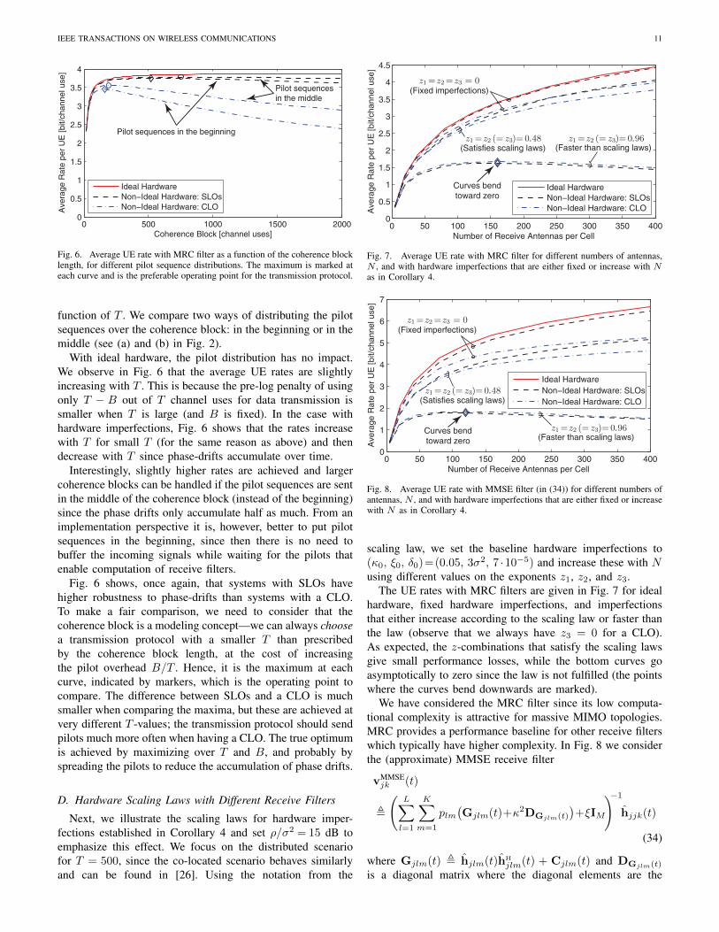
Fig. 6. Average UE rate with MRC filter as a function of the coherence blocklength, for different pilot sequence distributions. The maximum is marked ateach curve and is the preferable operating point for the transmission protocol.

function of T . We compare two ways of distributing the pilotsequences over the coherence block: in the beginning or in themiddle (see (a) and (b) in Fig. 2).

With ideal hardware, the pilot distribution has no impact.We observe in Fig. 6 that the average UE rates are slightlyincreasing with T . This is because the pre-log penalty of usingonly T − B out of T channel uses for data transmission issmaller when T is large (and B is fixed). In the case withhardware imperfections, Fig. 6 shows that the rates increasewith T for small T (for the same reason as above) and thendecrease with T since phase-drifts accumulate over time.

Interestingly, slightly higher rates are achieved and largercoherence blocks can be handled if the pilot sequences are sentin the middle of the coherence block (instead of the beginning)since the phase drifts only accumulate half as much. From animplementation perspective it is, however, better to put pilotsequences in the beginning, since then there is no need tobuffer the incoming signals while waiting for the pilots thatenable computation of receive filters.

Fig. 6 shows, once again, that systems with SLOs havehigher robustness to phase-drifts than systems with a CLO.To make a fair comparison, we need to consider that thecoherence block is a modeling concept—we can always choosea transmission protocol with a smaller T than prescribedby the coherence block length, at the cost of increasingthe pilot overhead B/T . Hence, it is the maximum at eachcurve, indicated by markers, which is the operating point tocompare. The difference between SLOs and a CLO is muchsmaller when comparing the maxima, but these are achieved atvery different T -values; the transmission protocol should sendpilots much more often when having a CLO. The true optimumis achieved by maximizing over T and B, and probably byspreading the pilots to reduce the accumulation of phase drifts.

D. Hardware Scaling Laws with Different Receive Filters

Next, we illustrate the scaling laws for hardware imper-fections established in Corollary 4 and set ρ/σ2 = 15 dB toemphasize this effect. We focus on the distributed scenariofor T = 500, since the co-located scenario behaves similarlyand can be found in [26]. Using the notation from the

0 50 100 150 200 250 300 350 4000

0.5

1

1.5

2

2.5

3

3.5

4

4.5

Number of Receive Antennas per Cell

Ave

rage

Rat

e pe

r U

E [b

it/ch

anne

l use

]

Ideal HardwareNon−Ideal Hardware: SLOsNon−Ideal Hardware: CLO

z1=z2 (= z3)=0.96(Faster than scaling laws)

z1=z2=z3 = 0(Fixed imperfections)

(Satisfies scaling laws)z1=z2 (= z3)=0.48

Curves bendtoward zero

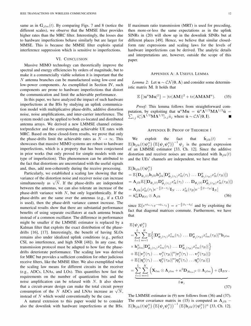
Fig. 7. Average UE rate with MRC filter for different numbers of antennas,N , and with hardware imperfections that are either fixed or increase with Nas in Corollary 4.

0 50 100 150 200 250 300 350 4000

1

2

3

4

5

6

7

Number of Receive Antennas per Cell

Ave

rage

Rat

e pe

r U

E [b

it/ch

anne

l use

]

Ideal HardwareNon−Ideal Hardware: SLOsNon−Ideal Hardware: CLO

z1=z2=z3 = 0(Fixed imperfections)

z1 3=z2 (= z )=0.96(Faster than scaling laws)

Curves bendtoward zero

(Satisfies scaling laws)z1=z2 (= z3)=0.48

Fig. 8. Average UE rate with MMSE filter (in (34)) for different numbers ofantennas, N , and with hardware imperfections that are either fixed or increasewith N as in Corollary 4.

scaling law, we set the baseline hardware imperfections to(κ0, ξ0, δ0)=(0.05, 3σ2, 7 ·10−5) and increase these with Nusing different values on the exponents z1, z2, and z3.

The UE rates with MRC filters are given in Fig. 7 for idealhardware, fixed hardware imperfections, and imperfectionsthat either increase according to the scaling law or faster thanthe law (observe that we always have z3 = 0 for a CLO).As expected, the z-combinations that satisfy the scaling lawsgive small performance losses, while the bottom curves goasymptotically to zero since the law is not fulfilled (the pointswhere the curves bend downwards are marked).

We have considered the MRC filter since its low computa-tional complexity is attractive for massive MIMO topologies.MRC provides a performance baseline for other receive filterswhich typically have higher complexity. In Fig. 8 we considerthe (approximate) MMSE receive filter

vMMSEjk (t)

,

(L∑l=1

K∑m=1

plm(Gjlm(t)+κ2DGjlm(t)

)+ξIM

)−1hjjk(t)

(34)

where Gjlm(t) , hjlm(t)hH

jlm(t) + Cjlm(t) and DGjlm(t)

is a diagonal matrix where the diagonal elements are the

IEEE TRANSACTIONS ON WIRELESS COMMUNICATIONS 12

same as in Gjlm(t). By comparing Figs. 7 and 8 (notice thedifferent scales), we observe that the MMSE filter provideshigher rates than the MRC filter. Interestingly, the losses dueto hardware imperfections behave similarly but are larger forMMSE. This is because the MMSE filter exploits spatialinterference suppression which is sensitive to imperfections.

VI. CONCLUSION

Massive MIMO technology can theoretically improve thespectral and energy efficiencies by orders of magnitude, but tomake it a commercially viable solution it is important that theN antenna branches can be manufactured using low-cost andlow-power components. As exemplified in Section IV, suchcomponents are prone to hardware imperfections that distortthe communication and limit the achievable performance.

In this paper, we have analyzed the impact of such hardwareimperfections at the BSs by studying an uplink communica-tion model with multiplicative phase-drifts, additive distortionnoise, noise amplifications, and inter-carrier interference. Thesystem model can be applied to both co-located and distributedantenna arrays. We derived a new LMMSE channel estima-tor/predictor and the corresponding achievable UE rates withMRC. Based on these closed-form results, we prove that onlythe phase-drifts limit the achievable rates as N → ∞. Thisshowcases that massive MIMO systems are robust to hardwareimperfections, which is a property that has been conjecturedin prior works (but only proved for simple models with onetype of imperfection). This phenomenon can be attributed tothe fact that distortions are uncorrelated with the useful signalsand, thus, add non-coherently during the receive processing.

Particularly, we established a scaling law showing that thevariance of the distortion noise and receiver noise can increasesimultaneously as

√N . If the phase-drifts are independent

between the antennas, we can also tolerate an increase of thephase-drift variance with N , but only logarithmically. If thephase-drifts are the same over the antennas (e.g., if a CLOis used), then the phase-drift variance cannot increase. Thenumerical results show that there are substantial performancebenefits of using separate oscillators at each antenna branchinstead of a common oscillator. The difference in performancemight be smaller if the LMMSE estimator is replaced by aKalman filter that exploits the exact distribution of the phase-drifts [16], [17]. Interestingly, the benefit of having SLOsremains also under idealized uplink conditions (e.g., perfectCSI, no interference, and high SNR [48]). In any case, thetransmission protocol must be adapted to how fast the phase-drifts deteriorate performance. The scaling law was derivedfor MRC but provides a sufficient condition for other judiciousreceive filters, like the MMSE filter. We also exemplified whatthe scaling law means for different circuits in the receiver(e.g., ADCs, LNAs, and LOs). This quantifies how fast therequirements on the number of quantization bits and thenoise amplification can be relaxed with N . It also showsthat a circuit-aware design can make the total circuit powerconsumption of the N ADCs and LNAs increase as

√N ,

instead of N which would conventionally be the case.A natural extension to this paper would be to consider

also the downlink with hardware imperfections at the BSs.

If maximum ratio transmission (MRT) is used for precoding,then more-or-less the same expectations as in the uplinkSINRs in (20) will show up in the downlink SINRs but atdifferent places [49]. Hence, we believe that similar closed-form rate expressions and scaling laws for the levels ofhardware imperfections can be derived. The analytic detailsand interpretations are, however, outside the scope of thispaper.

APPENDIX A: A USEFUL LEMMA

Lemma 2: Let u ∼ CN (0,Λ) and consider some determin-istic matrix M. It holds that

E|uHMu|2

= |tr(ΛM)|2 + tr(ΛMΛMH). (35)

Proof: This lemma follows from straightforward com-putation, by exploiting that uHMu = uHΛ1/2MΛ1/2u =∑i,j u

∗i [Λ

1/2MΛ1/2]i,j uj where u ∼ CN (0, I).

APPENDIX B: PROOF OF THEOREM 1

We exploit the fact that hjlk(t) =

Ehjlk(t)ψH

j (Eψjψ

H

j )−1

ψj is the general expressionof an LMMSE estimator [33, Ch. 12]. Since the additivedistortion and receiver noises are uncorrelated with hjlk(t)and the UEs’ channels are independent, we have that

Ehjlk(t)ψH

j = EDφj(t)

hjlkhH

jlk[DH

φj(τ1)x∗lk(τ1) . . . DH

φj(τB)x∗lk(τB)]

= ΛjlkE[Dφj(t)DH

φj(τ1)x∗lk(τ1) . . . Dφj(t)

DH

φj(τB)x∗lk(τB)]

= Λjlk[x∗lk(τ1)e−δ2 |t−τ1|IN . . . x∗lk(τB)e−

δ2 |t−τB |IN ]

= xH

lkDδ(t) ⊗Λjlk (36)

since Eeıφn,t1 e−ıφn,t2 = e−δ2 |t1−t2| and by exploiting the

fact that diagonal matrices commute. Furthermore, we havethat

EψjψH

j

=

L∑`=1

K∑m=1

E

[DH

φj(τ1)x∗`m(τ1) . . . DH

φj(τB)x∗`m(τB)]Hhj`m

× hH

j`m[DH

φj(τ1)x∗`m(τ1) . . . DH

φj(τB)x∗`m(τB)]

+ E[υH

j (τ1) . . .υH

j (τB)]H[υH

j (τ1) . . .υH

j (τB)]+ E[ηH

j (τ1) . . .ηH

j (τB)]H[ηH

j (τ1) . . .ηH

j (τB)]

=

L∑`=1

K∑m=1

(X`m ⊗Λj`m + κ2D|x`m|2 ⊗Λj`m

)+ ξIBN︸ ︷︷ ︸

,Ψj

.

(37)

The LMMSE estimator in (9) now follows from (36) and (37).The error covariance matrix in (15) is computed as Λjlk −Ehjlk(t)ψH

j (Eψjψ

H

j )−1

(Ehjlk(t)ψH

j )H [33, Ch. 12].

IEEE TRANSACTIONS ON WIRELESS COMMUNICATIONS 13

APPENDIX C: PROOF OF LEMMA 1

Since the effective channels vary with t, we follow theapproach in [15] and compute one ergodic achievable ratefor each t ∈ D. We obtain (19) by taking the average ofthese rates. The SINR in (20) is obtained by treating theuncorrelated inter-user interference and distortion noise asindependent Gaussian noise, which is a worst-case assumptionwhen computing the mutual information [39]. In addition, wefollow an approach from [38] and only exploit the knowl-edge of the average effective channel EvH

jk(t)hjjk(t) inthe detection, while the deviation from the average effectivechannel is treated as worst-case Gaussian noise with varianceE|vH

jk(t)hjjk(t)|2 − |EvH

jk(t)hjjk(t)|2.

APPENDIX D: PROOF OF THEOREM 2

The expressions in Theorem 2 are derived one at the time.For brevity, we use the following notations in the derivations:

Ajlk(t) =(xH

lkDδ(t) ⊗Λjlk

)Ψ−1j (38)

D|hjlk|2 = diag

(|h(1)jlk|

2, . . . , |h(N)jlk |

2

)(39)

Bjklm(t) = ΛjlmAjjk(t) (40)Mjklm(t) = DH

φj(t)Ajjk(t)

× [DT

φj(τ1)xlm(τ1) . . . DT

φj(τB)xlm(τB)]T. (41)

We begin with (21) and exploit that vjk(t) = hjlk(t) is anLMMSE estimate to see that

E‖vjk(t)‖2 = tr(Λjjk −Cjjk(t))

= tr((

xH

jkDδ(t) ⊗Λjjk

)Ψ−1j

(DH

δ(t)xjk ⊗Λjjk

)) (42)

which proves (21). Next, we exploit that hjjk(t) = Ajjk(t)ψjand note that

EvH

jk(t)hjjk(t) = tr(Ehjjk(t)ψH

j AH

jjk(t))

= tr((

xH

jkDδ(t) ⊗Λjjk

)AH

jjk(t))

= tr((

xH

jkDδ(t) ⊗Λjjk

)Ψ−1j

(DH

δ(t)xjk ⊗Λjjk

)) (43)

where the second equality follows from (36) and the thirdequality follows from the full expression of Ajjk(t) in(38). Observe that the expression (43) is the same as forE‖vjk(t)‖2 in (42).

Next, the second-order moment in (23) can be expanded as

E|vH

jk(t)hjlm(t)|2

= Etr(AH

jjk(t)hjlm(t)hH

jlm(t)Ajjk(t)ψjψH

j )

= tr

(AH

jjk(t)ΛjlmAjjk(t)(Ψj −Xlm ⊗Λjlm

))+ E

tr(MH

jklm(t)hjlmhH

jlmMjklm(t)hjlmhH

jlm)

+ κ2E

tr(AH

jjk(t)hjlmhH

jlmAjjk(t)(D|xlm|2 ⊗D|hjlm|2))

(44)

where the first term follows from computing separate ex-pectations for the parts of ψjψ

H

j that are independent of

hjlm(t)hH

jlm(t). The remaining two terms take care of thestatistically dependent terms. The middle term is simplified as

E

tr(MH

jklm(t)hjlmhH

jlmMjklm(t)hjlmhH

jlm)

= E|tr(ΛjlmMjklm(t))|2

+ E

tr(ΛjlmMjklm(t)ΛjlmMH

jklm(t)) (45)

by computing the expectation with respect to hjlm usingLemma 2 in Appendix A. The first expectation in (45) is nowcomputed by expanding the expression as

E|tr(ΛjlmMjklm(t))|2 = E∣∣∣tr(Bjklm(t)

× [DT

φj(τ1)xlm(τ1) . . . DT

φj(τB)xlm(τB)]TDH

φj(t)

)∣∣∣2= E

N∑n1=1

B∑b1=1

[Bjklm(t)Eb1 ]n1n1xlm(τb1)eıφn1,τb1 e−ıφn1,t

×N∑

n2=1

B∑b2=1

[EH

b2BH

jklm(t)]n2n2x∗lm(τb2)e

−ıφn2,τb2 eıφn2,t

=

∑n1,n2,b1,b2

[Bjklm(t)Eb1 ]n1n1[EH

b2BH

jklm(t)]n2n2

× xlm(τb1)x∗lm(τb2)Eeı(φn1,τb1

−φn1,t−φn2,τb2+φn2,t)

(46)

where Ebi = ebi ⊗ IN and ebi ∈ CB×1 is the bith column ofIB . The phase-drift expectation depends on the use of a CLOor SLOs:

Eeı(φn1,τb1

−φn1,t−φn2,τb2

+φn2,t)

=

e−

δ2 |τb1−τb2 |, if a CLO,

e−δ2 |τb1−τb2 |, if SLOs and n1 = n2,

e−δ2 |t−τb1 |e−

δ2 |t−τb2 |, if SLOs and n1 6= n2.

(47)

Since xlm(τb1)x∗lm(τb2)e−δ2 |τb1−τb2 | = [Xlm]b1,b2 =

eH

b1Xlmeb2 in the case of a CLO, (46) becomes

∑n1,n2,b1,b2

[Bjklm(t)Eb1 ]n1n1[EH

b2BH

jklm(t)]n2n2eH

b1Xlmeb2

=∑n1,n2

eH

n1Bjklm(t)(Xlm ⊗ en1e

H

n2)BH

jklm(t)en2

(48)

where en ∈ CN×1 is the nth column of IN (recall also thedefinitions of Eb and eb above).

Next, we note that e−δ2 |t−τb|xlm(τb) = [DH

δ(t)xlm]b. In the

IEEE TRANSACTIONS ON WIRELESS COMMUNICATIONS 14

case of SLOs, (46) then becomes

∑n1,n2,b1,b2n1 6=n2

[Bjklm(t)Eb1 ]n1n1[EH

b2BH

jklm(t)]n2n2

× [DH

δ(t)xlm]b1 [xH

lmDδ(t)]b2

+∑n,b1,b2

[Bjklm(t)Eb1 ]nn[EH

b2BH

jklm(t)]nn[Xlm]b1,b2

=∣∣∣∑n,b

[Bjklm(t)Eb]nn[DH

δ(t)xlm]b

∣∣∣2+∑n,b1,b2

[Bjklm(t)Eb1 ]nn[EH

b2BH

jklm(t)]nn

× [Xlm −DH

δ(t)xlmxH

lmDδ(t)]b1,b2

=∣∣tr(Ajjk(t)(DH

δ(t)xlm ⊗Λjlm))∣∣2 +

∑n

eH

nBjklm(t)

×((Xlm −DH

δ(t)xlmxH

lmDδ(t))⊗ eneH

n

)BH

jklm(t)en.

(49)

The second expectation in (45) is computed along the samelines as in (37) and becomes

Etr(ΛjlmMjklm(t)ΛjlmMH

jklm(t))= tr

(ΛjlmAjjk(t)(Xlm ⊗Λjlm)AH

jjk(t)).

(50)

It remains to compute the last term in (44). We exploitthe following expansion of diagonal matrices: D|xlm|2 =∑Bb=1 |xlm(τb)|2ebeH

b and D|hjlm|2 =∑Nn=1 |eH

nhjlm|2eneHn,

where eb is the bth column of IB and en is the nth columnof IN . Plugging this into the last term in (44) yields

∑b,n

|xlm(τb)|2E|hH

jlmAjjk(t)(eb ⊗ eneH

n)hjlm|2

=∑b,n

∣∣xlm(τb)|2|tr(ΛjlmAjjk(t)(eb ⊗ eneH

n))∣∣2

+∑b,n

|xlm(τb)|2tr(ΛjlmAjjk(t)(eb ⊗ eneH

n)

×Λjlm(eH

b ⊗ eneH

n)AH

jjk(t))

=∑n

eH

nΛjlmAjjk(t)(D|xlm|2 ⊗ eneH

n)AH

jjk(t)Λjlmen

+ tr(ΛjlmAjjk(t)(D|xlm|2 ⊗Λjlm)AH

jjk(t))

(51)

where the first equality follows from Lemma 2 and thesecond equality from reverting the matrix expansions whereverpossible. Plugging (45)–(51) into (44) and utilizing Xlm +κ2D|xlm|2 = Xlm, we obtain (23) by removing the specialnotation that was introduced in the beginning of this appendix.

Finally, we compute the expectation in (24) by noting that

E|vH

jk(t)υj(t)|2 = Etr(AH

jjk(t)Υj(t)Ajjk(t)ψjψH

j )

= κ2L∑l=1

K∑m=1

plm

×(

tr(AH

jjk(t)ΛjlmAjjk(t)(Ψj −Xlm ⊗Λjlm

))+ Etr(MH

jklm(t)D|hjlm|2Mjklm(t)hjlmhH

jlm)

+ κ2Etr(AH

jjk(t)D|hjlm|2Ajjk(t)(D|xlm|2 ⊗D|hjlm|2))).

(52)

The first equality follows by taking the expectation withrespect to υj(t) for fixed channel realizations. The secondequality follows by taking separate expectations with respectto the terms of Υj = κ2

∑Ll=1

∑Km=1 plmD|hjlm|2 and ψjψ

H

j

that are independent. These give the first term in (52) while thelast two terms take care of the statistically dependent terms.

The expectation in the middle term of (52) is computed as

Etr(MH

jklm(t)D|hjlm|2Mjklm(t)hjlmhH

jlm)

=∑n

E|hH

jlmMH

jklm(t)eneH

nhjlm|2

=∑n

E|eH

nΛjlmMH

jklm(t)en|2

+∑n

EeH

nΛjlmeneH

nMjklm(t)ΛjlmMH

jklm(t)en

= tr(ΛjlmAjjk(t)(Xlm ⊗Λjlm)AH

jjk(t))

+∑n

eH

nΛjlmAjjk(t)(Xlm ⊗ eneH

n)AH

jjk(t)Λjlmen

(53)

where the first equality follows from the same diagonal matrixexpansion as in (51), the second equality is due to Lemma 2(and that diagonal matrices commute), and the third equalityfollows from computing the expectation with respect to phase-drifts as in (37) and then reverting the matrix expansionswherever possible.

Similarly, we have

Etr(AH

jjk(t)D|hjlm|2Ajjk(t)(D|xlm|2 ⊗D|hjlm|2))

=∑

n1,n2,b

|xlm(τb)|2E|hH

jlmen1eH

n1Ajjk(t)(eb ⊗ en2

eH

n2)hjlm|2

=∑

n1,n2,b

|xlm(τb)|2(∣∣tr(Λjlmen1

eH

n1Ajjk(t)(eb ⊗ en2

eH

n2))∣∣2

+ tr(Λjlmen1

eH

n1Ajjk(t)(ebe

H

b ⊗ en2eH

n2Λjlm)AH

jjk(t)))

=∑n1

eH

n1ΛjlmAjjk(t)(D|xlm|2 ⊗ en1

eH

n1)AH

jjk(t)Λjlmen1

+ tr(ΛjlmAjjk(t)(D|xlm|2 ⊗Λjlm)AH

jjk(t))

(54)

where the first equality follows from the same diagonal matrixexpansions as above, the second equality follows from Lemma2 (and that diagonal matrices commute), and the third equalityfrom reverting the matrix expansions wherever possible.

By plugging (53) and (54) into (52) and utilizing Xlm +κ2D|xlm|2 = Xlm, we finally obtain (24).

IEEE TRANSACTIONS ON WIRELESS COMMUNICATIONS 15

APPENDIX E: PROOF OF COROLLARY 3

This corollary is obtained by dividing all the termsin SINRjk(t) by N2

A2 and inspecting the scaling behav-ior as N → ∞. Using the expressions in Theorem 2and utilizing that Ψ−1j = Ψ

−1j ⊗ IN

A, we observe that

ξA2

N2 E‖vjk(t)‖2 = ξA2

N2 tr(F ⊗ INA

) = ξAN tr(F) = O( 1

N ),

where F =(xH

jkDδ(t)⊗Λ(A)jjk

)Ψ−1j

(Dδ(t)xjk⊗Λ

(A)jjk

).

Similarly, it is straightforward but lengthy to prove thatA2

N2E|vH

jk(t)υj(t)|2 = O( 1N ). The only terms in the SINR

that remain as N →∞ are A2

N2 (E‖vjk(t)‖2)2 = Sigjk andA2

N2E|vH

jk(t)hjlm(t)|2 = Intjklm +O( 1N ).

APPENDIX F: PROOF OF COROLLARY 4

The first step of the proof is to substitute the new pa-rameters into the SINR expression in (20) and scale allterms by 1/N1+z3δ0 minτ |t−τ |. Since the distortion noiseand receiver noise terms normally behave as O(N), it isstraightforward (but lengthy) to verify that the (scaled) dis-tortion noise and receiver noise terms go to zero whenN → ∞. Similarly, the signal term in the numerator whichnormally behave as O(N2), will after the scaling behaveas O(N1−2max(z1,z2)−z3δ0 minτ |t−τ |). In the case of SLOs,the second-order interference moments E|vH

jk(t)hjlm(t)|2in the denominator exhibit the same scaling as the signalterm. The scaling law in (30) then follows from that we wantthe signal and interference terms to be non-vanishing in theasymptotic limit; that is, 1 − 2 max(z1, z2) − z3δ0 minτ |t −τ | > 1. In the case of a CLO, the second-order interferencemoments behave as O(N1−2max(z1,z2)) and do not depend onz3. To make the signal and interference terms have the samescaling and be non-vanishing, we thus need to set z3 = 0 andmax(z1, z2) ≤ 1

2 .

REFERENCES

[1] M. K. Karakayali, G. J. Foschini, and R. A. Valenzuela, “Networkcoordination for spectrally efficient communications in cellular systems,”IEEE Wireless Commun. Mag., vol. 13, no. 4, pp. 56–61, Aug. 2006.

[2] D. Gesbert, S. Hanly, H. Huang, S. Shamai (Shitz), O. Simeone, andW. Yu, “Multi-cell MIMO cooperative networks: A new look atinterference,” IEEE J. Sel. Areas Commun., vol. 28, no. 9, pp. 1380–1408, Dec. 2010.

[3] E. Bjornson and E. Jorswieck, “Optimal resource allocation in coordi-nated multi-cell systems,” Foundations and Trends in Communicationsand Information Theory, vol. 9, no. 2-3, pp. 113–381, 2013.

[4] H. Holma and A. Toskala, LTE for UMTS: Evolution to LTE-Advanced,Wiley, 2nd edition, 2011.

[5] J. Hoydis, K. Hosseini, S. ten Brink, and M. Debbah, “Making smartuse of excess antennas: Massive MIMO, small cells, and TDD,” BellLabs Technical Journal, vol. 18, no. 2, pp. 5–21, Sep. 2013.

[6] R. Baldemair, E. Dahlman, G. Fodor, G. Mildh, S. Parkvall, Y. Selen,H. Tullberg, and K. Balachandran, “Evolving wireless communications:Addressing the challenges and expectations of the future,” IEEE Veh.Technol. Mag., vol. 8, no. 1, pp. 24–30, Mar. 2013.

[7] E. G. Larsson, F. Tufvesson, O. Edfors, and T. L. Marzetta, “MassiveMIMO for next generation wireless systems,” IEEE Commun. Mag.,vol. 52, no. 2, pp. 186–195, Feb. 2014.

[8] China Mobile Research Institute, “C-RAN: The road towards greenRAN,” Tech. Rep., White Paper, Oct. 2011.

[9] T. L. Marzetta, “Noncooperative cellular wireless with unlimitednumbers of base station antennas,” IEEE Trans. Wireless Commun.,vol. 9, no. 11, pp. 3590–3600, Nov. 2010.

[10] F. Rusek, D. Persson, B. K. Lau, E. G. Larsson, T. L. Marzetta,O. Edfors, and F. Tufvesson, “Scaling up MIMO: Opportunities andchallenges with very large arrays,” IEEE Signal Process. Mag., vol. 30,no. 1, pp. 40–60, Jan. 2013.

[11] J. Hoydis, S. ten Brink, and M. Debbah, “Massive MIMO in the UL/DLof cellular networks: How many antennas do we need?,” IEEE J. Sel.Areas Commun., vol. 31, no. 2, pp. 160–171, Feb. 2013.

[12] H. Q. Ngo, E. G. Larsson, and T. L. Marzetta, “Energy and spectralefficiency of very large multiuser MIMO systems,” IEEE Trans.Commun., vol. 61, no. 4, pp. 1436–1449, Apr. 2013.

[13] E. Bjornson, L. Sanguinetti, J. Hoydis, and M. Debbah, “Designingmulti-user MIMO for energy efficiency: When is massive MIMO theanswer?,” in Proc. IEEE WCNC, Apr. 2014, pp. 242–247.

[14] S. K. Mohammed and E. G. Larsson, “Per-antenna constant envelopeprecoding for large multi-user MIMO systems,” IEEE Trans. Commun.,vol. 61, no. 3, pp. 1059–1071, Mar. 2013.

[15] A. Pitarokoilis, S. K. Mohammed, and E. G. Larsson, “Uplink perfor-mance of time-reversal MRC in massive MIMO systems subject to phasenoise,” IEEE Trans. Wireless Commun., vol. 14, no. 2, pp. 711–723, Feb.2015.

[16] R. Krishnan, M. R. Khanzadi, N. Krishnan, A. Graell i Amat, T. Eriks-son, N. Mazzali, and G. Colavolpe, “On the impact of oscillator phasenoise on the uplink performance in a massive MIMO-OFDM system,”Available online, http://arxiv.org/abs/1405.0669.

[17] E. Bjornson, J. Hoydis, M. Kountouris, and M. Debbah, “MassiveMIMO systems with non-ideal hardware: Energy efficiency, estimation,and capacity limits,” IEEE Trans. Inf. Theory, vol. 60, no. 11, pp. 7112–7139, Nov. 2014.

[18] T. Schenk, RF Imperfections in High-Rate Wireless Systems: Impactand Digital Compensation, Springer, 2008.

[19] A. Mezghani, N. Damak, and J. A. Nossek, “Circuit aware design ofpower-efficient short range communication systems,” in Proc. IEEEISWCS, Sep. 2010, pp. 869–873.

[20] M. Wenk, MIMO-OFDM Testbed: Challenges, Implementations, andMeasurement Results, Series in microelectronics. Hartung-Gorre, 2010.

[21] D. Petrovic, W. Rave, and G. Fettweis, “Effects of phase noise on OFDMsystems with and without PLL: Characterization and compensation,”IEEE Trans. Commun., vol. 55, no. 8, pp. 1607–1616, Aug. 2007.

[22] H. Mehrpouyan, A. A. Nasir, S. D. Blostein, T. Eriksson, G. K.Karagiannidis, and T. Svensson, “Joint estimation of channel andoscillator phase noise in MIMO systems,” IEEE Trans. Signal Process.,vol. 60, no. 9, pp. 4790–4807, Sep. 2012.

[23] G. Durisi, A. Tarable, and T. Koch, “On the multiplexing gain of MIMOmicrowave backhaul links affected by phase noise,” in Proc. IEEE ICC,June 2013, pp. 3209–3214.

[24] W. Zhang, “A general framework for transmission with transceiverdistortion and some applications,” IEEE Trans. Commun., vol. 60, no.2, pp. 384–399, Feb. 2012.

[25] E. Bjornson, M. Matthaiou, and M. Debbah, “Massive MIMO systemswith hardware-constrained base stations,” in Proc. IEEE ICASSP, May2014, pp. 3142–3146.

[26] E. Bjornson, M. Matthaiou, and M. Debbah, “Circuit-aware design ofenergy-efficient massive MIMO systems,” in Proc. IEEE ISCCSP, May2014, pp. 101–104.

[27] X. Gao, O. Edfors, F. Rusek, and F. Tufvesson, “Massive MIMO in realpropagation environments,” IEEE Trans. Wireless Commun., 2014, Toappear, Available: http://arxiv.org/abs/1403.3376.

[28] A. Farhang, N. Marchetti, L. E. Doyle, and B. Farhang-Boroujeny,“Filter bank multicarrier for massive MIMO,” in Proc. IEEE VTC Fall,2014.

[29] H. Yang and T. L. Marzetta, “Total energy efficiency of cellular largescale antenna system multiple access mobile networks,” in Proc. IEEEOnlineGreenComm, Oct. 2013, pp. 27–32.

[30] E. Dahlman, S. Parkvall, J. Skold, and P. Beming, 3G Evolution: HSPAand LTE for Mobile Broadband, Academic Press, 2nd edition, 2008.

[31] M. Biguesh and A. B. Gershman, “Downlink channel estimation incellular systems with antenna arrays at base stations using channelprobing with feedback,” EURASIP J. Appl. Signal Process., vol. 2004,no. 9, pp. 1330–1339, 2004.

[32] H. Yin, D. Gesbert, M. Filippou, and Y. Liu, “A coordinated approachto channel estimation in large-scale multiple-antenna systems,” IEEE J.Sel. Areas Commun., vol. 31, no. 2, pp. 264–273, Feb. 2013.

[33] S. M. Kay, Fundamentals of Statistical Signal Processing: EstimationTheory, Prentice Hall, 1993.

[34] J. H. Kotecha and A. M. Sayeed, “Transmit signal design for optimalestimation of correlated MIMO channels,” IEEE Trans. Signal Process.,vol. 52, no. 2, pp. 546–557, Feb. 2004.

IEEE TRANSACTIONS ON WIRELESS COMMUNICATIONS 16

[35] E. Bjornson and B. Ottersten, “A framework for training-based es-timation in arbitrarily correlated Rician MIMO channels with Riciandisturbance,” IEEE Trans. Signal Process., vol. 58, no. 3, pp. 1807–1820, Mar. 2010.

[36] T. Yoo and A. Goldsmith, “Capacity and power allocation for fadingMIMO channels with channel estimation error,” IEEE Trans. Inf. Theory,vol. 52, no. 5, pp. 2203–2214, May 2006.

[37] G. Durisi, A. Tarable, C. Camarda, R. Devassy, and G. Montorsi,“Capacity bounds for MIMO microwave backhaul links affected byphase noise,” IEEE Trans. Commun., vol. 62, no. 3, pp. 920–929, Mar.2014.

[38] M. Medard, “The effect upon channel capacity in wireless communica-tions of perfect and imperfect knowledge of the channel,” IEEE Trans.Inf. Theory, vol. 46, no. 3, pp. 933–946, May 2000.

[39] B. Hassibi and B. M. Hochwald, “How much training is needed inmultiple-antenna wireless links?,” IEEE Trans. Inf. Theory, vol. 49, no.4, pp. 951–963, Apr. 2003.

[40] J. Jose, A. Ashikhmin, T. L. Marzetta, and S. Vishwanath, “Pilotcontamination and precoding in multi-cell TDD systems,” IEEE Trans.Commun., vol. 10, no. 8, pp. 2640–2651, Aug. 2011.

[41] R. Muller, M. Vehkapera, and L. Cottatellucci, “Blind pilot decontami-nation,” IEEE J. Sel. Topics Signal Process., vol. 8, no. 5, pp. 773–786,Oct. 2014.

[42] C. Risi, D. Persson, and E. G. Larsson, “Massive MIMO with 1-bitADC,” Available online, http://arxiv.org/abs/1404.7736.

[43] I. Song, M. Koo, H. Jung, H.-S. Jhon, and H. Shinz, “Optimization ofcascode configuration in CMOS low-noise amplifier,” Micr. Opt. Techn.Lett., vol. 50, no. 3, pp. 646–649, Mar. 2008.

[44] D. Petrovic, W. Rave, and G. Fettweis, “Common phase error dueto phase noise in OFDM-estimation and suppression,” in Proc. IEEEPIMRC, Sept. 2004, pp. 1901–1905.

[45] K.-G. Park, C.-Y. Jeong, J.-W. Park, J.-W. Lee, J.-G. Jo, and C. Yoo,“Current reusing VCO and divide-by-two frequency divider for quadra-ture LO generation,” IEEE Microw. Wireless Compon. Lett., vol. 18, no.6, pp. 413–415, June 2008.

[46] J. R. Wilkerson, Passive Intermodulation Distortion in Radio FrequencyCommunication Systems, Ph.D. thesis, North Carolina State University,2010.

[47] Further advancements for E-UTRA physical layer aspects (Release 9),3GPP TS 36.814, Mar. 2010.

[48] M. R. Khanzadi, G. Durisi, and T. Eriksson, “Capacity ofmultiple-antenna phase-noise channels with common/separate oscil-lators,” IEEE Trans. Commun., 2014, To appear, Available:http://arxiv.org/abs/1409.0561.

[49] E. Bjornson, M. Bengtsson, and B. Ottersten, “Optimal multiusertransmit beamforming: A difficult problem with a simple solutionstructure,” IEEE Signal Process. Mag., vol. 31, no. 4, pp. 142–148,July 2014.