14 Random Variables II - Dept of Math, CCNY

263

14 Random Variables IIHomer: My son, a genius!? How does it happen?Dr.J: Well, genius, like intelligence, is usually the result of heredityand environment.Homer: [stares blankly]Dr.J: Although in some cases, it's a total mystery.

From: The Simpsons

14.1 Continuous Random Variables

In the last chapter we considered discrete random variables. In order to apply probability modelsto a wider range of phenomena we must extend the concepts to deal with continuous randomvariables. The first difficulty is a fundamental one - How do we compute probabilities? Forexample, if X represents the length of time, in years, that a person survives after receiving atreatment for a particular type of cancer, then we can think of X as having values in the interval(0, ∞ ). What is the meaning of ( 5.75)P X = ? If we interpret this literally, the only reasonableanswer is “zero”. Indeed, if we require that the person live exactly 5.75 years after treatment andnot a moment more or less, then this is so restrictive as to be impossible. In practice, it is morereasonable to ask for the probability that a person lives between say 5.5 and 6 years. In general, ifX is a continuous random variable the probability ( )P X x= is zero for any specific x . Non-zeroprobabilities may arise when we consider the probability that X falls into an interval [ , ]a b , whichwe write as ( )P a X b≤ ≤ . We need to understand how the latter probabilities are computed.

The probability histogram is the key to understanding how probabilities are computed in thecontinuous case. For discrete random variables we hardly gave a thought to the width of the barsused in our histograms. We will now be less casual about this and will adjust the bar width toconvey some useful information. Consider first a binomial random variable X having 10n = and

.7p = . The probability histogram is shown below.

Probability Histogram

00.050.1

0.150.2

0.250.3

0 1 2 3 4 5 6 7 8 9 10

X = #successes

Unlike some earlier histograms for the binomial distribution, we have drawn this with no gapsbetween the bars. As each bar extends ½ unit to the right and left of the value of X , the width ofeach bar is one and therefore the area of each box is the same as the height of the box, which is the

14 Random Variables II

264

probability. Thus, in this picture we have two ways of thinking about the probability. The heightor the area of each bar represents the probability of the corresponding value of X . The arearepresentation is useful for visualizing probabilities of the form ( )P a X b≤ ≤ , for example

(5 7) ( 5) ( 6) ( 7)P X P X P X P X≤ ≤ = = + = + = . The latter sum is easy to visualize as the area ofthe three shaded rectangles shown below.

Probability Histogram

0

0.05

0.1

0.15

0.2

0.25

0.3

0 1 2 3 4 5 6 7 8 9 10

# success

prob

The idea of using areas to compute probabilities is the key to computing with continuous randomvariables. The stair-like histogram for the discrete random variable is replaced by a smooth curveand the areas under this curve give the probabilities associated with the random variable. Thesmooth curve defining the outline of the histogram is called the probability density function. Itsdefinition is given by

Definition 14.1 (Probability Density Function) A probability density function of a continuousrandom variable X is a function ( )f x with the following two properties:

a) For all x , ( ) 0f x ≥ .

b) The area under the graph of ( )f x from −∞ to +∞ is one.!

If these conditions hold then for any real numbers a and b , the probability that X will lie in theinterval [ , ]a b , denoted by ( )P a X b≤ ≤ , is equal to the area under the graph of ( )f x over theinterval [ , ]a b . The assignment of probabilities described in Definition 14.1 is often referred to asa probability distribution for the random variable X.

One technical point to observe is that in computing probabilities for continuous random variables itmakes no difference whether we consider closed or open intervals. In other words,

( ) ( )P a X b P a X b< < = ≤ ≤ . This is usually false for discrete random variables, since taking intoaccount the possibility that X a= may make a difference in the two probabilities. Indeed theevent ( ) or ( ) or ( )a X b a X b X a X b≤ ≤ = < < = = . The last three events are mutually exclusiveand therefore ( ) ( ) ( ) ( )P a X b P a X b P X a P X b≤ ≤ = < < + = + = . As we stated above, for


265

continuous random variables ( ) 0P X x= = and so in the continuous case we have the equality( ) ( )P a X b P a X b≤ ≤ = < < . Similar arguments apply if only one of the ≤ signs is replaced by

strict inequality. We will often make use of this freedom in adjusting the boundaries of theinterval, particularly when considering complements.

14.2 The Uniform Distribution

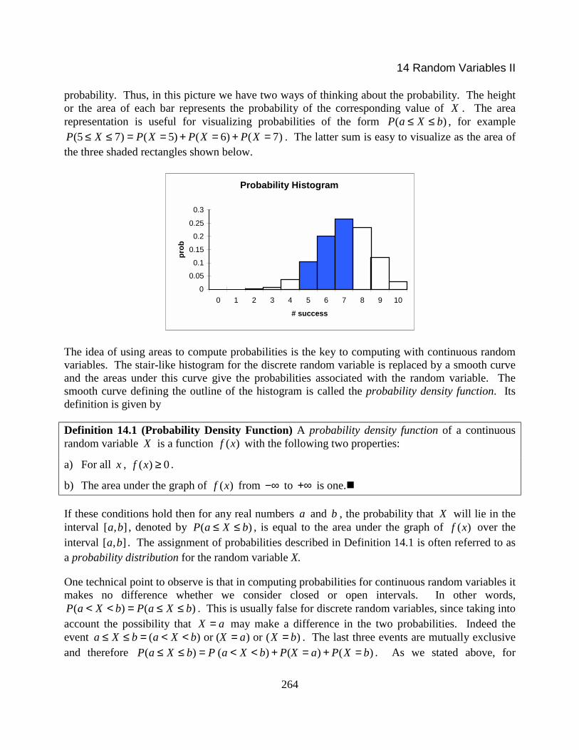
Our focus in this chapter will be on two continuous random variables, the uniform distribution andthe normal distribution. Consider the density function given by

0 if 0( ) 1 if 0 1

0 if 1

xf x x

x

<= ≤ ≤ <

.

The graph of this density function is shown below. A random variable having this density functionis said to have a uniform distribution.

Areas under the curve represent probabilities. Thus for instance, there is zero probability ofobtaining a value of X in the interval from 1 to 2 since the area under that portion of the curve iszero. On the other hand, the area of the shaded region extending from 0.5X = to 0.75X = is0.25 and so (.5 .75) .25P X≤ ≤ = . In general, for this random variable, if a and b are anynumbers in the interval [0,1] with a b< , then ( )P a X b b a≤ ≤ = − . Note that the ordinate on theabove graph does not represent a probability, but rather a quantity called a probability density,which is the area of the region, i.e. the probability, divided by the length of the interval.

There is a simple physical model for a random variable with this density function. Suppose weaim darts at the number line, but vertical barriers prevent the darts from hitting anywhere except inthe interval [0,1]. If we do not aim at any particular location in [0,1], then the chance of the dartlanding in any subinterval [ , ]a b is dependent on the length b a− of that interval. There is less of


a chance of hitting a small interval than a larger one. The uniform density defined above says thatthe chance is exactly equal to the length of the subinterval.

The uniform density plays an important role in creating computer simulations for arbitrary randomvariables. For example, suppose we can produce random numbers X in the interval [0,1] that aredistributed according to the uniform density. If X denotes any such number, then by ourdiscussion above (0 0.5) 0.5P X≤ ≤ = and (0.5 1) 0.5P X< ≤ = . Thus these two mutuallyexclusive events can be thought of as representing the outcomes of “Heads” and “Tails” for thetoss of a coin and we can use this to construct a coin-tossing simulation. Similar, although morecomplicated constructions can be used to simulate other discrete and continuous random variables.See the tech notes for a more detailed description related to Excel. We will not describe the exactmethod that Excel and other programs use to generate these random numbers.

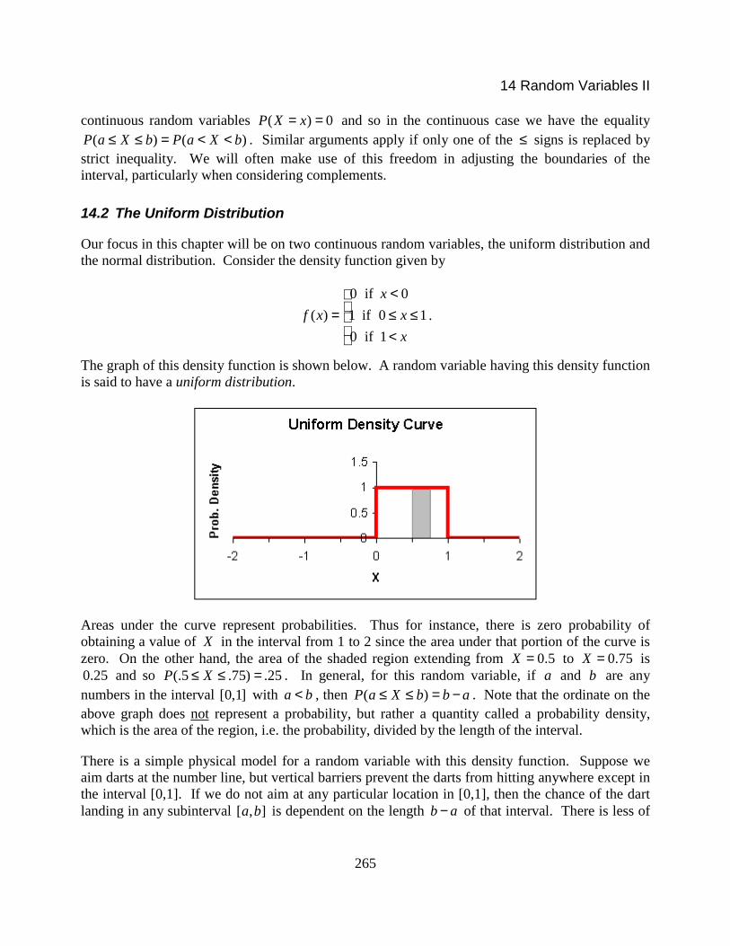
Many biological problems dealing with the spatial distribution of a species lead to theconsideration of uniform densities in two and three spatial dimensions, and sometimes a timedimension as well (i.e. multivariate uniform distributions). In the biological literature uniformdispersal patterns are often referred to as random dispersion. The picture below shows asimulation of such a pattern in a 10 by 10-rectangular region. The points were obtained

!!!!

266

mathematically by selecting the x coordinates using a uniform distribution on the interval 0 to 10and making a similar random selection for the y coordinate. Note the occasional clustering ofpoints. Recognizing excessive clustering patterns is often very important evidence in analyzingoutbreaks of diseases or environmentally caused illness. The Poisson distribution is a prime tool indeciding whether cluster patterns deviate significantly from those produced by uniform dispersal.

Uniform Scatter: 100 Points

0

10

0 10x

y

Figure 14.1


267

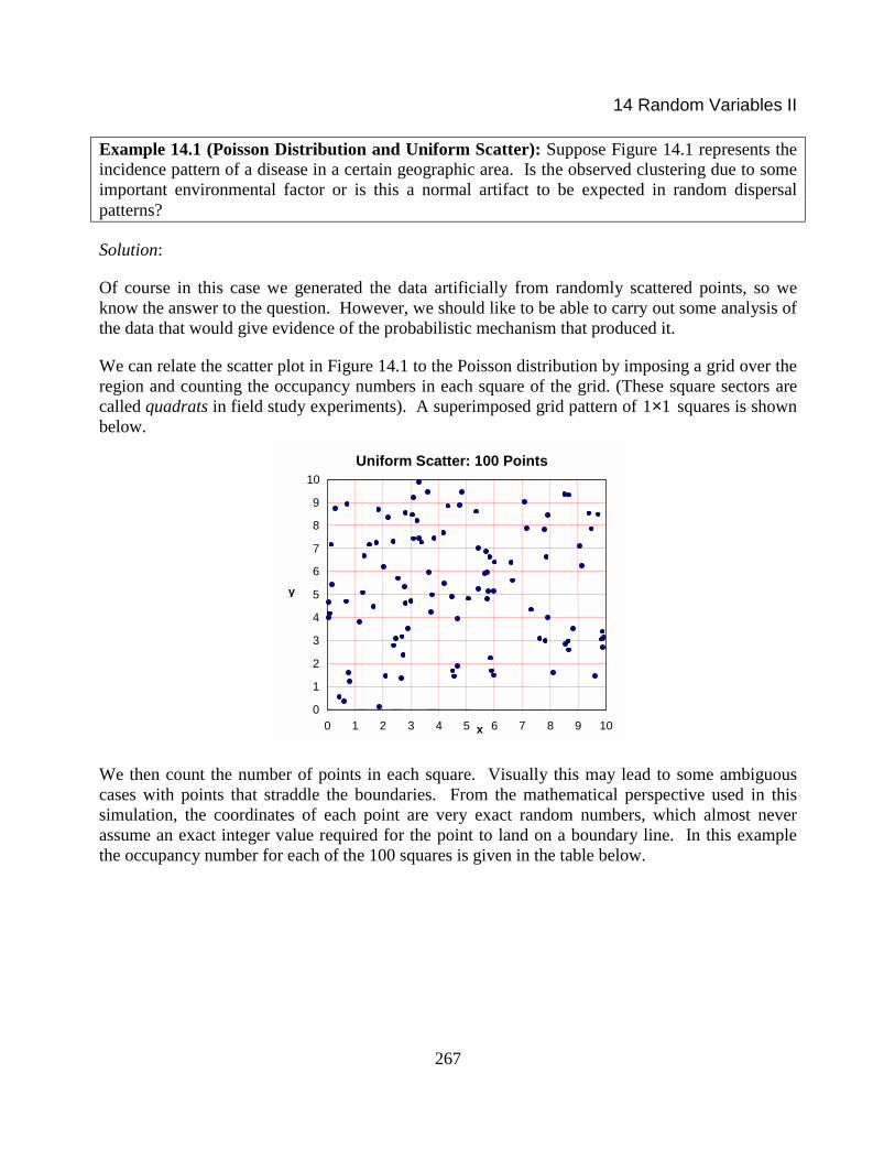
Example 14.1 (Poisson Distribution and Uniform Scatter): Suppose Figure 14.1 represents theincidence pattern of a disease in a certain geographic area. Is the observed clustering due to someimportant environmental factor or is this a normal artifact to be expected in random dispersalpatterns?

Solution:

Of course in this case we generated the data artificially from randomly scattered points, so weknow the answer to the question. However, we should like to be able to carry out some analysis ofthe data that would give evidence of the probabilistic mechanism that produced it.

We can relate the scatter plot in Figure 14.1 to the Poisson distribution by imposing a grid over theregion and counting the occupancy numbers in each square of the grid. (These square sectors arecalled quadrats in field study experiments). A superimposed grid pattern of 1 1× squares is shownbelow.

Uniform Scatter: 100 Points

0

1

2

3

4

5

6

7

8

9

10

0 1 2 3 4 5 6 7 8 9 10x

y

We then count the number of points in each square. Visually this may lead to some ambiguouscases with points that straddle the boundaries. From the mathematical perspective used in thissimulation, the coordinates of each point are very exact random numbers, which almost neverassume an exact integer value required for the point to land on a boundary line. In this examplethe occupancy number for each of the 100 squares is given in the table below.


268

Occupancy Numbers9 0 0 0 3 1 0 0 1 2 08 2 1 2 2 2 1 0 1 0 27 1 2 1 4 1 1 0 2 0 26 0 1 1 0 0 2 2 1 0 15 1 1 2 1 1 5 1 0 0 04 3 1 1 3 1 2 0 2 0 03 1 1 3 0 1 0 0 1 1 32 0 0 2 0 0 1 0 1 3 11 2 0 2 0 3 2 0 0 1 10 2 1 0 0 0 0 0 0 0 0

0 1 2 3 4 5 6 7 8 9

We then make a tally of the number of cells that are unoccupied, the number of cells that have oneoccupant, etc. For example there is one cell with five “hits”, one cell with four “hits”, seven cellswith three “hits”. This is tabulated below.

Occupancy # 0 1 2 3 4 5Frequency 40 32 19 7 1 1

Table 14.1

So far we have just spent a lot of effort tabulating our results. Now we assume that the points arescattered via a uniform dispersal mechanism. Since our grid contains 100 squares the chance of apoint landing in a given square is .01 (all squares, having the same area, are equally likely to be hitif the dispersal is uniform). Focusing still on a particular square, the probability of k out of 100points landing in this square is the probability that k successes will occur in 100 trials of abinomial random variable with .01p = . In Chapter 13, section 13.4 we have seen that a Poissonrandom variable may be used to approximate such a binomial distribution. The appropriatePoisson distribution will have 100(.01) 1npλ = = = . Notice that 1λ = is also the average numberof points in each 1 1× square, in the sense that we are tossing 100 points onto a grid with 100boxes, so that each box will contain on average one point.

Using the formula for the probabilities of a Poisson distribution, we obtain the followingprobabilities for a square to have no “hits”, one “hit” etc. These probabilities are then multipliedby 100 to obtain the expected number of squares in the grid that would have the given number of“hits”. This is the third row in the table below.


269

Occupancy # 0 1 2 3 4 5Predicted PoissonFrequency ( 1λ = ) 0.37 0.37 0.18 0.06 0.02 0.003

Predicted Frequency 37 37 18 6 2 .3

The predicted frequency pattern is then compared to the observed pattern in Table 14.1. In thiscase the agreement seems quite good and one might take this as reasonable evidence that the pointswere scattered by a uniform dispersal mechanism. In more ambiguous situations one might needto use the chi-square test, which is a statistical procedure measuring whether there is sufficientagreement between the observed and predicted values. Additional simulations of this sort may becarried out using the file scatter.xls.

We have here another instance of the hypothesis testing procedure mentioned earlier in Chapter 11and which we will discuss in more detail in Chapter 16. The logic of the method is to assume thedispersal mechanism is uniform, draw from that the conclusion that the occupancy pattern willfollow a Poisson distribution and then compare the data with this prediction. If the fit betweenmodel and data is good we can't be absolutely certain the dispersal pattern is uniform, but we haveevidence to support it. If the fit were poor, by the standards we choose to establish, we wouldlikely reject the hypothesis of uniform or random dispersal and look at other mechanisms thatmight have led to the observed pattern.

The analysis above requires a large amount of computation. A somewhat abbreviated, but lessreliable alternative is described in exercise 3.!

14.3 The Standard Normal Distribution

The normal density is the most important probability density function, with the widest range ofapplicability. In discussing the so-called standard normal distribution it is customary to use theletter Z for the random variable and z for its values.

Definition 14.2 (The Standard Normal Density): The function 2 / 21( )

2zf z e

π−= is called the

standard normal density function. A random variable Z has a standard normal distribution if forany real numbers a and b the probability ( )P a Z b≤ ≤ is equal to the area under the graph of

( )f z between a and b .!

Because of the shape of the graph of ( )f z (see Figure 14.2 below) the density is often called thebell-shaped curve, although many other mathematical expressions can produce graphs with asimilar appearance. As we will see, the Bell Curve Rule (Rule 7.1) derives from properties of thestandard normal density. The density ( )f z is also called the gaussian density, after C. F. Gauss,


270

the German mathematician whose investigations in the 19th century established the fundamentalimportance of the normal distribution.

Figure 14.2

In Figure 14.2 the shaded area between one and two gives the probability that Z falls in theinterval [1, 2]. Unlike the case of the uniform distribution, this area cannot be computed by simplegeometric considerations. Indeed integral calculus is needed to compute the area. You will recallfrom calculus that areas under curves may be obtained as the value of a definite integral. In thiscase we have

22 / 2

1

1(1 2)2

zP Z e dzπ

−≤ ≤ = ∫ .

Unfortunately, no matter how skillful you are at evaluating integrals the latter integral cannot beexpressed in closed form in terms of the usual elementary functions. Numerical methods(Riemann sums etc.) are needed to approximate the value to any desired accuracy. From apractical viewpoint, these results have been tabulated, or a computer may be used in which asuitable routine has been provided for this computation. Here we will consider the use of tables,such as those given in section B.3. The tech notes describe the appropriate Excel functions.

The tables give cumulative probabilities or areas under the density curve from −∞ to z . This isindicated by the schematic at the top of the table. To obtain the result for the example

( 1.65)P Z < , we look at the first table of section B.3. In the z column locate the first two digits1.6. The digits 0, 1, 2, … running along the top of the table are used to specify the second decimalplace (except for the last row 3.± , where the top row gives the first decimal place). Scanningalong the row beginning 1.6 to the column under 5, we read the entry .9505. This represents thearea under the density curve to the left of 1.65z = and therefore gives the probability that

1.65Z < . For negative values of Z we use the 2nd table of section B.3.


271

Before we examine some examples showing how to use the tables to compute probabilities, it isimportant to recall that, as for any continuous density function, the total area under the graph of

( )f z is one.

Example 14.2: Compute the following probabilities by finding the area of suitable regions underthe normal density curve.

a) ( .73)P Z < −

b) ( 1)P Z >

c) (1 2)P Z< <

d) ( 2)P Z <

e) A value 0z so that 0( ) 0.1P Z z> = .

Solution:

First, note that based on our comments after Definition 14.1, we would obtain the same answers ifwe replaced any of the strict inequalities above with ≤ .

a) Use the second table in section B.3 as described above. You find ( 0.73) .2327P Z < − = .Notice this is less than 1/2, as it should be, since the area involved is only a portion of the areato the left of the origin. If we had carelessly used the table for positive Z to obtain an answerof .7673 this type of simple reality check would have alerted us to an error.

b) The tables give probabilities of the form ( )P Z a≤ . The complement of the event ( 1)P Z > is( 1)P Z ≤ , which has probability 0.8413, using the entry for 1.00z = in section B.3. Thus the

Rule of Complements (Rule 10.5) gives ( 1) 1 .8413 0.1587P Z > = − = .

c) The desired probability is the area between 1z = and 2z = . The pictogram below shows howthis area can be related to the tabulated cumulative areas by appropriate subtraction.

= −

Thus (1 2) ( 2) ( 1) .9772 .8413 .1359P Z P Z P Z< < = < − < = − = .


272

d) The condition 2Z < is the same as 2 2Z− < < . Using the same analysis as in c) we canevaluate the probability as

( 2) ( 2 2) ( 2) ( 2) .9772 .0228 .9544P Z P Z P Z P Z< = − < < = < − < − = − = .

e) This problem involves reverse table look-up. This means we are given a probability and haveto find the z value that is associated with this probability. In this case, the probability we aregiven is of the type 0( )P Z z> and the table does not list these. However, by considering thecomplementary event we have that 0( ) 1 0.1 .9P Z z< = − = . Using the body of the table, notthe z value column, we find the nearest probability listing to .9. This is found in section B.3and corresponds to the z entry 0 1.28z = , for which the listed probability is .8997.!

14.4 Normal Distributions

In the last section we considered the special standard normal distribution. In most applicationsmore general normal distributions are needed. We describe how these are obtained and how theyare related to the standard normal density.

To begin, we must say something about the mean and standard deviation for continuous randomvariables. We recall from chapter 13 that these quantities are numbers that describe the theoreticalaverage and standard deviation for data that can be modeled by the discrete random variable.Similar theoretical averages and standard deviations can be defined for continuous randomvariables. The precise definitions extend the formulas in Definitions 13.4 and 13.5 of Chapter 13by replacing the summations in those formulas with suitable definite integrals. We will not go intothe technical details, as they do not add a great deal to our goal of understanding how to use theseconcepts. However, it is important to state the results for the standard normal distribution.

Theorem 14.1: If Z is the standard normal distribution then 0Zµ = and 1Zσ = .!

This result has an important visual interpretation in terms of the graph of the density function( )f z . Referring to Figure 14.2, the mean 0µ = is clearly the center and peak point in the density

graph. Notice also that the graph has two inflection points. The figure suggests, and a littlecalculus confirms, that these occur at the points 1z = ± . Thus, the distance of the inflection pointsfrom the center is equal to the standard deviation. Moreover, since the standard deviation is one, avalue such as 2z = is two standard deviations above the mean zero; 2.5z = − is 2.5 standarddeviations below the mean zero, etc. With this in mind we can give a working definition of anarbitrary normal distribution.


273

Definition 14.3 (Normal Distribution): A random variable X has a normal distribution withmean µ and standard deviation σ , if its density curve arises from the standard normal density by:

a) shifting the latter so it is centered around µ

b) contracting or expanding the standard normal density curve so it has inflection points at µ σ±

c) rescaling the height of the standard normal density so that the total area beneath it remainsone.!!!!

According to this definition, a normal distribution is described by giving its mean µ and standarddeviation σ . It is convenient to designate such a quantity using the notation ( , )X N µ σ= , whichis an abbreviation for the statement that the random variable X has a normal distribution withmean µ and standard deviation σ . The figure below shows examples of such normaldistributions with densities determined by 5µ = and 2,1, 0.5, 0.25σ = respectively. In all casesof course the total area under the curve is one. Notice that in order to achieve this constant areathe ordinate or density rises as the central portion of the graph narrows, in accord with property c)in the definition.

Normal Density: µµµµ=5, σσσσ =2

0

0.5

1

1.5

2

-1 5

X

dens

ity

Normal Density: µµµµ=5, σσσσ =1

0

0.5

1

1.5

2

-1 5

X

dens

ity

Normal Density: µµµµ=5, σσσσ =.5

0

0.5

1

1.5

2

-1 5

X

dens

ity

Normal Density: µµµµ=5, σσσσ =.25

0

0.5

1

1.5

2

-1 5

X

dens

ity

Figure 14.3


274

Definition 14.4 ( z -score): Suppose x is a value of a random variable X that has a normaldistribution with mean µ and standard deviationσ . The z -score of x is the number of standarddeviations of x from the mean value µ . It is given by

xz µσ−= .!

Example 14.3: If (10, 3)X N= what are the z -scores of 12x = and 7.5x = ?

Solution:

Using Definition 14.4, the z -score for 12x = is 12 10 .673

z −= ≈ and the z -score for 7.5x = is

7.5 10 .833

z −= ≈ − .!

The z -score gives the number of standard deviations of a value of X from the mean. For thestandard normal distribution we saw that the value of Z also equaled the number of standarddeviations from the mean. The connection between these facts is the basis of the computation ofprobabilities for normal distributions.

Theorem 14.2: If X has a normal distribution with mean µ and standard deviation σ then the

z -scores derived from X by the equation xz µσ−= have a standard normal distribution.

Moreover for any X values a and b if az and bz denote the z -scores of a and b respectivelywe have

( ) ( )a bP a X b P z Z z< < = < <

( ) ( )aP a X P z Z< = <

( ) ( )bP X b P Z z< = < .!

The importance of this theorem cannot be overstated. In essence it says that for a normaldistribution the standard deviation is the appropriate measuring stick needed to computeprobabilities.

Example 14.4: For the random variable (10, 3)X N= of Example 14.3 find the (7.5 12).P X< <

Solution:

Although not essential, the reader is encouraged to make a simple sketch of the bell-shapeddistribution of X with the mean value clearly marked and an indication of the region whose area


275

needs to be computed. In this example the following sketch would be sufficient and indicates wemight expect a probability of approximately 0.5.

According to Theorem 14.2, to compute (7.5 12)P X< < we need the z -scores of the endpoints ofthe interval. These were computed in Example 14.3 as .83z = − for 7.5x = and .67z = for

12x = . Therefore by Theorem 14.2 we have

(7.5 12) ( .83 .67) ( 0.67) ( 0.83) .7517 .2033 .5484P X P Z P Z P Z< < = − < < = < − < − = − =

which agrees fairly well with our guess based on the sketch.!

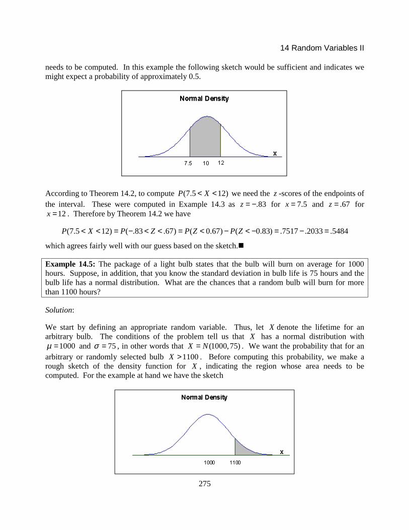
Example 14.5: The package of a light bulb states that the bulb will burn on average for 1000hours. Suppose, in addition, that you know the standard deviation in bulb life is 75 hours and thebulb life has a normal distribution. What are the chances that a random bulb will burn for morethan 1100 hours?

Solution:

We start by defining an appropriate random variable. Thus, let X denote the lifetime for anarbitrary bulb. The conditions of the problem tell us that X has a normal distribution with

1000µ = and 75σ = , in other words that (1000,75)X N= . We want the probability that for anarbitrary or randomly selected bulb 1100X > . Before computing this probability, we make arough sketch of the density function for X , indicating the region whose area needs to becomputed. For the example at hand we have the sketch


276

and one might venture an estimate of 0.25 or less for the probability. To actually compute( 1100)P X > we proceed as in Theorem 14.2. We need the z -score of the value 1100x = . This is

1100 1000 1.3375

z −= ≈ . Thus by the theorem we have

( 1100) ( 1.33) 1 ( 1.33) 1 .9082 .0918P X P Z P Z> = > = − < = − = .

In rough terms, there is slightly less than a 10% chance that the bulb will last as long as 1100hours.!

Theorem 14.2 provides the basis of the Bell Curve Rule (Rule 7.1).

Theorem 14.3 (Bell Curve Rule): If X has a normal distribution with mean µ and standarddeviation σ then the following statements hold:

a) There is a 68% probability that X will yield a value within one standard deviation of themean.

b) There is a 95% probability that X will yield a value within 1.96 standard deviations of themean.

c) There is a 99.7% probability that X will yield a value within 3 standard deviations of themean.

Proof:

We illustrate b). The proofs of the others are similar. The event that X is within 1.96 standarddeviations of its mean signifies that the value of X falls in the interval 1.96µ σ− to 1.96µ σ+ .We therefore want ( )P a X b≤ ≤ where 1.96a µ σ= − and 1.96b µ σ= + . The z -scores of a and

b are 1.96a µσ− = − and 1.96b µ

σ− = respectively. Therefore,

( ) ( 1.96 1.96) .9750 .0250 .95P a X b P Z≤ ≤ = − ≤ ≤ = − = .!

The precise spread of 1.96 standard deviations given in b) is often rounded, as we have done inChapter 7, to two standard deviations when we apply the rule to data. Recall that the randomvariable X is a model for the description of data and the data, average and standard deviation areapproximations to the theoretical values. Thus, for any data exhibiting an approximate bell-shapedhistogram the Bell Curve Rule should give approximate percentages of the data lying within one,two and three standard deviations of the mean.

Example 14.6: For the normal distributions shown in Figure 14.3 estimate or use the tables to find(4 6)P X< < .

Solution:


277

In the top left panel we have (5,2)X N= . The z -scores of 4 and 6 are -0.5 and 0.5 respectively.Thus (4 6) ( .5 .5) .383P X P Z< < = − < < = , a value obtained from the tables. In the upper rightpanel we have (5,1)X N= . The z -scores of 4 and 6 are then -1 and 1 so the Bell Curve Rule(Theorem 14.3) applies, yielding (4 6) .68P X< < = . For the lower left panel, (5,0.5)X N= andtherefore the z -scores are -2 and 2. The Bell Curve Rule gives the estimate of .95 for theprobability. Finally in the last panel, (5,.25)X N= and the z -scores are -4 and 4. These zvalues are not given in the table, but since we are given entries for 3.9z = ± we may use theseprobabilities to infer that to three decimal places ( 4) 1P Z < = and ( 4) 0P Z < − = . This impliesthat (4 6) 1P X< < = , as is suggested by the graph.!

Example 14.7: The scores on a test used for admissions to a selective school are approximatelynormally distributed with a mean of 320 and a standard deviation of 50 (The maximum possiblegrade is 500). What cut-off score should be set so that only the top 10% of applicants will beaccepted?

Solution:

Let X be the score of a randomly selected student. The assumptions in the problem imply that wemay assume (320,50)X N= . We want to find a value x of X so that only 10% of students scorehigher than this value. In other words, we want x to satisfy ( ) .10P X x> = . The z -score for the

unknown value x is 32050

xz −= . Using the relationship between probabilities for X and

probabilities for Z we have 320.10 ( ) ( )50

xP X x P Z −= > = > . However, in Example 14.2e) we

showed how to find the value 0z such that 0( ) .10P Z z> = . We found that 0 1.28z = . Thus the

z -score 320 1.2850

x − = . Solving for x yields the cut-off score of 384.

Having solved the problem, the solution can be explained more directly. For the Z distribution,there is only a 10% chance of a value exceeding 1.28. This is the content of Example 14.2e). Foran arbitrary normal distribution X , the z -score is the number of standard deviations from themean. Therefore, we can assert that there is a 10% chance that a value of X will be more than1.28 standard deviations above the mean. Hence, the cut-off point must be 1.28 standarddeviations above the mean 320. This gives 320 1.28(50) 384x = + = .!

14.5 The Normal Approximation to the Binomial

The normal distribution was actually discovered at the end of the 18th century in the attempt to findgood numerical approximations to cumulative binomial probabilities, particularly when thenumber of trials n was large. Although from the computational point of view the result is nolonger needed if a computer is available, the result shows an important relationship between thesetwo types of random variables. The upshot of those investigations is the following theorem.


278

Theorem 14.4 (Normal-Binomial Approximation I): Suppose n is large and p is neither veryclose to zero nor very close to one, (we'll make this precise below). The binomial distribution Xwith n independent trials and probability of success p can be approximated by a normaldistribution with the same mean ( )np and the same standard deviation ( )npq as X . More

explicitly, denoting by ( , )Y N np npq= the normal distribution with mean np and standard

deviation npq , we have for any a and b that ( ) ( )P a X b P a Y b≤ ≤ ≈ ≤ ≤ .!

Roughly speaking, the theorem asserts that when n is large the binomial distribution behaves likea normal distribution with mean np and standard deviation npq .

Example 14.8: Suppose that X is a binomial distribution with 100n = and 0.4p = . UseTheorem 14.4 to estimate (30 45)P X≤ ≤ .

Solution:

The mean value of X is 40np = and the standard deviation is 100(.4)(.6) 4.9npq = ≈ .Theorem 14.4 asserts that the normal distribution (40, 4.9)Y N= can be used to provide a goodapproximation to (30 45)P X≤ ≤ . The graph below, which superimposes the normal densitycurve on the binomial histogram, illustrates the construction.

Probability Histograms

0

0.02

0.040.06

0.08

0.1

30 33 36 39 42 45

# Successes

Prob

abili

ty

BinomialNormal

Figure 14.4

As we discussed in section 14.1, the binomial probability between 30 and 45 can be found byadding the areas of the rectangular probability bars (since these have been expanded to width one).The picture clearly shows that this area is very close to the area under the corresponding normaldistribution curve. Let's perform the approximation and then, using Excel, compare the answer toan exact result.


279

According to the theorem, (30 45) (30 45)P X P Y≤ ≤ ≈ ≤ ≤ , where (40, 4.9)Y N= . The normalprobability is computed using the methods of the previous section. We find the z -scores for theendpoints 30 and 45. These are

30 40 2.044.9− = − and 45 40 1.02

4.9− = .

Therefore, (30 45) ( 2.04 1.02) .8461 .0207 .8254P Y P Z≤ ≤ = − ≤ ≤ = − = . The latter number is ourapproximation. The exact value using the binomdist function is .8541. The estimate differs byabout .03 or 3% points - good, but not spectacular. In fact we can do better!!

Example 14.9 (The Continuity Correction): We show how to improve the approximation in thelast example using a method known as the continuity correction.

Solution:

Consider again Figure 14.4 reproduced with slight modification below.

The rectangular probability bars at the beginning and end have been split. The black portion ofthese bars is part of the area that is included in the probability (30 45)P X≤ ≤ , which adds theareas of all the rectangles. However, the approximation (30 45)P Y≤ ≤ includes only the areaunder the normal curve from 30 to 45, and the black bars are not included in this area since theyextend from the center of the box (30 or 45) to the left or right endpoints (29.5 or 40.5). Thus itwould seem that our estimation of the binomial area would fall short of the actual value. This wasindeed the case in Example 14.8. We can attempt to correct this by extending the interval overwhich we compute the area under the normal curve. Instead of going from 30 to 45 we shouldcompute the area from the lower boundary of the left rectangle, 29.5, to the upper boundary of theright rectangle, 40.5. Thus we make the refined estimate

(30 45) (29.5 45.5) ( 2.14 1.12) .8524P X P Y P Z≤ ≤ ≈ ≤ ≤ = − ≤ ≤ = ,

which agrees much more closely with the exact answer .8541.!


280

The estimation technique described in Example 14.9 is called the continuity correction, since it isthe result of trying to fit a continuous graph to a step-like histogram. We include this in oursecond version of the Normal Approximation theorem. When you want to compute the binomialprobabilities with greater accuracy, you should use this continuity correction. If great accuracy isnot so important, use the cruder approximation given in Theorem 14.4.

Theorem 14.5 (Normal-Binomial Approximation II): If X has a normal distribution with30n > and the probability p satisfies 5np > and 5nq > (where 1q p= − ) then the normal

distribution ( , )Y N np npq= can be used to approximate probabilities for X . Namely, for any aand b , the continuity correction gives

( ) ( 0.5 0.5)P a X b P a Y b≤ ≤ ≈ − ≤ ≤ + !

Theorem 14.5 clarifies the conditions under which the approximation is valid. The conditionrelated to p , namely that both np and nq are larger than 5, asserts that the expected number ofsuccesses and expected number of failures should not be too small. The figure below illustrateswhat happens when 5np < .

Binomial: n=100, p=.03 & Normal

00.050.1

0.150.2

0.25

0 1 2 3 4 5 6 7 8 9

# Successes

Prob

abili

ty

BinomialNormal

The fit is very poor. The binomial distribution is quite skewed in a case such as this and asymmetric distribution such as the normal cannot adequately account for this. In this situation wehave seen in Chapter 13 section 13.4 that the Poisson distribution gives an easy to computenumerical approximation to the binomial.

Example 14.10: If a coin is tossed 500 times would it be surprising to get 270 or more heads?Explain.

Solution:

The number of heads obtained has a binomial distribution with 500n = and .5p = . According toour approximation theorems this random variable is approximately normal with mean 250np =and standard deviation 11.2npq = . An outcome exceeding 270 heads would be more than 1.8


281

standard deviations above the expected value. From the tables of the standard normal distributionthe chance of this happening is approximately 0.04. Thus, such a result would be consideredsomewhat unusual.!

14.6 Tech Notes

Simulated values of the uniform distribution and various normal distributions can be obtained byusing the Data Analysis tools and the option Random Number Generation, as described in Chapter13. Random numbers in the interval [0,1] can also be generated directly in a spreadsheet using thecommand =rand().

Probabilities for normal distributions can be obtained from the file distributions.xls, using theNormal sheet. The file also contains sheets that show the comparison of the binomial and normaldistributions. On any spreadsheet the commands normsdist and normdist can be used to findcumulative normal probabilities for the standard normal distribution and for an arbitrary normaldistribution. The function wizard can assist you in entering the correct arguments for thesefunctions.

Example 14.11: Use Excel commands to compute (15 27)P X≤ ≤ where X is normal with20µ = and 4σ = .

Solution:

We must compute the answer using our usual procedure of expressing the probability(15 27)P X≤ ≤ as a difference of two cumulative probabilities. This can be accomplished by

entering the commands shown below in column A, rows 1 to 3. Column B shows the output fromthese commands.

A B1 =normdist(27,20,4,true) .9599412 =normdist(15,20,4,true) .105653 =a1-a2 .854291

!

In some of our examples it has been necessary to find a z value such that ( )P Z z≤ equaled aspecified probability. We called this reverse table look-up. Mathematically this processcorresponds to the computation of an inverse function. This inverse process is programmed inExcel through the command normsinv. For example, the solution of Example 14.2e) can beobtained by first converting the question to the cumulative probability statement 0( ) .9P Z z≤ =and then entering the command =normsinv(.9).


282

14.7 Summary

Many random quantities produce numerical values that fluctuate over an interval of values, forexample:

• the annual rainfall at a locale

• a randomly selected person’s height

• a randomly selected person’s age at death

• the site of an accident on a long stretch of highway

• time between exposure to a disease and onset of illness

• the midday CO concentration at an air quality monitoring site

These examples illustrate quantities that may be thought of as continuous random variables, X .To create a probability model for such random variables, we use a density function ( )f x . This isa positive valued function for which the total area under the graph is one. Probabilities of the form

( )P a X b≤ ≤ are computed using areas under the graph of the density function ( )f x .

The uniform density and the normal density are two important examples of such densityfunctions. With a uniform density, probabilities are “spread” over a certain interval in such a waythat an outcome has equal chance of landing in subintervals of the same length. We say in thiscase that the random variable has a uniform distribution. The accident site on a long stretch ofmore-or-less similar highway might conform to this probability model; any mile-long portion ofroad should be equally likely to be the site of an accident. The uniform distribution on [0,1] formsthe basis of all computer simulations of random processes.

In contrast, for a normal density the outcomes cluster near the peak of the density curve, withvalues farther from the center being less likely to occur. The exact computation of probabilitiesusing a normal density makes use of the mean and standard deviation of the random variable.Specifically, when X has a normal density curve (so we say X has a normal distribution or isnormally distributed) we associate with each value x of the random variable a z-score, defined asthe number of standard deviations of x above or below its mean. These z-scores have probabilitiesdescribed by the standard normal density, with mean zero and standard deviation one, for whichextensive tables or computer code can be used to find probabilities.

Normal or approximately normal distributions are common models for continuous data. Often, theapplicability of a normal model is based on analogy to well-known examples that exhibit suchbehavior. When a large amount of data is available, the fit of the normal model can be assessedusing a histogram or other graphical means. Certain discrete random variables can also beapproximated using a normal model. Besides being computationally useful, such results offerimportant theoretical insight into the behavior of the underlying random variables. For example, anormal distribution gives good approximations to the binomial distribution when n is large and p isneither very close to zero or one.


283

14.8 Exercises

1. a) Using Definition 14.1 verify that the graphs in panels A and B below are each densityfunctions for random variables, called respectively X and Y .

Density Curve (A)

00.25

0.50.75

1

-2 -1 0 1 2 3

X

Prob

. Den

sity

Density Curve (B)

00.25

0.50.75

1

-2 -1 0 1 2 3

Y

Prob

. Den

sity

b) For each of the random variables described in a) find the probability that the variable takeson a value in the interval [1, 1.5].

c) Find a value 0x such that 0( ) .9P X x≤ =

d) Find a value 0y such that 0( ) .9P Y y≤ =

2. During a certain hour of the day, an average of 200 cars pass through a toll plaza. Assume thearrival times are spread uniformly throughout the hour and the cars are traveling to theirdestinations independently of each other.

a) For a fixed one-minute time period, what is the probability p that a randomly selected carwill arrive at the plaza during that minute, as opposed to any other minute in the one-hourblock?

b) For a fixed one-minute time period explain why the number of cars from the group of 200arriving during that one-minute time period can be modeled by a Poisson random variablewith 3.33λ ≈ .

c) Dividing the hour into 60 consecutive one-minute subintervals, based on b) estimate inapproximately how many of these intervals there will be 0, 1, 2, … 6, 7, 8 cars arriving.

d) The following table gives the results of a simulation of the process described in thisproblem (200 cars arriving at random times during a one-hour time interval). The top rowspecifies the number of cars arriving in a given minute and the bottom row tabulates thenumber of one-minute intervals with this number of cars arriving.

# of cars k arriving during one minute 0 1 2 3 4 5 6 7 8# of one-minute intervals with k cars arriving 3 6 8 17 15 4 4 1 2

Table 14.2Compare the frequencies in row 2 for the simulated data with the prediction based on c). Doyou think the simulated data conforms to the model?


284

3. From Chapter 13 we know that a Poisson random variable X satisfies Xµ λ= and Xσ λ= .It follows that the square of the standard deviation, the variance of X , satisfies 2varX Xσ λ= = .

In other words, if X has a Poisson distribution then varX Xµ= . Ecologists use the ratio 2s

x,

the so-called index of dispersion, as a means of testing how well the data of an occupancypattern conforms to a Poisson distribution. A value of this ratio that is close to one is evidencesupporting a Poisson occupancy pattern.

a) Compute the index of dispersion for the occupancy data in Table 14.1 (page 268).

b) Compute the index of dispersion for the occupancy data in Table 14.2 above.

c) How strongly do the indices of dispersion computed in a) and b) support the hypothesis ofa Poisson distribution?

4. The number of years a person lives after receiving treatment for a type of cancer is acontinuous random variable, which we denote by T . In many cases this random variable has adensity function of the form

0 if 0( )

if 0t

tf t

e tαα −

≤=

>(14.1)

Here α is a constant greater than zero and t is measured in years. We will assume that ( )f tsatisfies Definition 14.1, and hence can be used as a density function.

a) Sketch on the same axes the graphs of the density functions (14.1) when 0.5α = and when0.25α = .

b) If 0.5α = find (0 2)P T≤ ≤ . What does the latter probability signify in terms of thepatient's survival following treatment?

c) It can be shown that the expected survival time Tµ for a random variable having thedensity (14.1) is 1 α . When .5α = , what is the probability that a patient will survive formore than twice the average time? (Hint: Consider the complementary event.)

5. If Z has a standard normal distribution find

a) ( 1.6)P Z <

b) ( .52)P Z > −

c) (1.2 2.24)P Z≤ <

d) ( 2.5)P Z <

6. If X has a normal distribution with mean µ =18 and 3σ = find

a) (16 20)P X≤ ≤


285

b) ( 19)P X ≤

7. If X has a binomial distribution with 50n = and .3p = use the normal approximation (withcontinuity correction) to estimate

a) ( 12)P X ≤

b) (10 18)P X≤ ≤

8. Let Z have a standard normal distribution. Find a value of 0z such that

a) 0( ) 0.6P Z z< ≈

b) 0( ) 0.6P Z z< ≈

c) If (5,2)X N= use a) to find a value 0x such that 0( ) 0.6P X x< ≈

9. Suppose that on average 3% of a manufacturer's output is defective. The manufacturer'sdistributor will return any shipments that contain more than 4.5% defectives. If shipments aremade in lots of 1000, what is the probability that a shipment will be returned? (Hint: 4.5%defectives in a shipment of 1000 means 45 defectives. How likely is this, given themanufacturer's claim?)

10. Suppose the annual rainfall in N.Y. is normally distributed with a mean of 42 inches per yearand a standard deviation of 4 inches. What is the probability that in a given year the rainfall,X , is between 36 and 48 inches?

11. Suppose it is known that only 90% of the people who reserve a seat on a flight actually showup. If a plane holds 220 passengers, explain, by using a suitable binomial distribution, why theairline is fairly confident that they can reserve 235 seats and still provide a seat for everyonewho shows.

12. a) The manufacturer of a TV picture tube knows that with customary usage the averagelifetime for a tube is 5.4 years, with a standard deviation of 1.1 years. Assuming thelifetime is normally distributed find the percentage of tubes that will fail before 5 years.

b) If the manufacturer wants to give a full refund warranty for defective tubes, how longshould the warranty period be so that at most 0.4% of the tubes are returned underwarranty?

13. Suppose the yearly income of workers in a certain industry is normally distributed with meanequal to $30,000 and standard deviation $4250.

a) If a worker is chosen at random, what is the probability that the worker's income will bebetween $25,000 and $40,000?

b) What is the probability that the worker's income will exceed $25,000?


286

c) Find the income level I so that only 1% of workers will have incomes exceeding I .

14. Assume that the time required to complete a certain medical procedure is normally distributedwith mean 3 hours and standard deviation of 20 minutes.

a) What is the probability that the procedure will be completed in less than 2.5 hours?

b) Assume the procedure is done on an outpatient basis. A friend accompanies the patient,but wishes to leave the facility while the procedure is in progress in order to complete someerrands. However, the friend wants to be 98% certain she will be back before theprocedure is done. What is the maximum length of time she should be gone?

15. Good-n-Tasty candy bars have a weight of 6 oz. listed on the package. In practice, thepackaged bars are not individually weighed, so the 6-oz. weight listed on the package may beincorrect. In particular, the bar may actually weigh less than 6 oz. Suppose the actual weightsare normally distributed with a mean of 6.25 oz. and a standard deviation of 0.1 oz.

a) What fraction of the bars will actually have a weight below the 6-oz. weight listed on thepackage?

b) In order to comply with anti-fraud statutes, the manufacturer must make sure that no morethan 1 in 1000 bars has an actual weight below 6 oz.. Assuming that the standard deviationof the production process remains the same (0.1 oz.), what is the smallest value for themean weight that will meet the anti-fraud requirements?

16. In 1977 a very large study (Hypertension Detection and Follow-up Program) produced datashowing that the diastolic blood pressure reading in adults has a normal distribution with amean of 85 mm Hg and a standard deviation of about 13. (The units refer to the height in amercury (Hg) column typically used to measure pressure.)

a) What fraction of the population would be classified as mildly hypertensive (i.e. having highblood pressure) if the cutoff for this category was a diastolic pressure in excess of 95 mmHg?

b) What fraction of the population would be classified as having severe hypertension if thecutoff for this category was a diastolic pressure in excess of 115 mm Hg?

17. The diastolic blood pressure of an individual varies from one reading to the next, even whenthe person is resting. Suppose a person actually has moderate hypertension, meaning hisaverage diastolic pressure is 105 mm Hg. If studies have shown that pressure readings forindividuals show a standard deviation of 7 mm Hg, what is the probability that a single readingfor this individual will yield a pressure reading below 95, and hence a misclassification of theindividual as only mildly hypertensive?

18. a) Use Excel's random number generator to obtain 1000 random values drawn from thestandard normal distribution.

b) Find the mean and standard deviation of the numbers you obtained in a). These numbersshould be close to zero and one respectively.


287

c) Test the conclusion of the Bell Curve Rule (Theorem 14.3) for the data generated in a).

19. a) Use Excel to generate 1000 random numbers X from a normal distribution (1,1)N . Placethese in column A of a worksheet. Generate another 1000 random numbers Y from adistribution that is (2,1)N and place these in column B of the same sheet.

b) In column C compute the sum X Y+ of the numbers generated in columns A and B above.Find the mean and standard deviation of these numbers and then using the Bell Curve Ruletest whether the sums appear to conform to a normal distribution.

c) In column D compute the product XY of the random numbers obtained in columns A andB. Repeat the instructions in b) for the numbers in column D.

20. If X is a random variable taking on positive values only and log X (natural logarithm) has anormal distribution, the random variable X is said to have a lognormal distribution. Thelognormal distribution arises in finance and risk management, as well as in ecologicalapplications involving the dispersion of hazardous wastes and other pollutants.

a) Use Excel’s random number generator to simulate 1000 values from the standard normaldistribution. Using the latter numbers obtain random numbers X whose natural logarithmhas the standard normal distribution.

b) Make a histogram of the lognormally distributed random numbers X obtained in a), usinga small bin width (for example 0.5).

c) Is the histogram in a) symmetric? Is it skewed? If so, which way? Find the median andthe mean of the lognormally distributed numbers X . Is the relationship between the meanand median reflective of the skewness of the distribution?

Documents

14 Random Variables II - Dept of Math, CCNY