Embed Size (px)
Citation preview

14
Hydrogenic Atoms
Contents
14.1 Introduction 251
14.2 Two Important Principals of Physics 252
14.3 The Wave Equations 253
14.4 Quantization Conditions 254
14.5 Geometric Symmetry SO(3) 257
14.6 Dynamical Symmetry SO(4) 261
14.7 Relation With Dynamics in FourDimensions 264
14.8 DeSitter Symmetry SO(4, 1) 266
14.9 Conformal Symmetry SO(4, 2) 270
14.9.1 Schwinger Representation 27014.9.2 Dynamical Mappings 27114.9.3 Lie Algebra of Physical Operators 274
14.10 Spin Angular Momentum 275
14.11 Spectrum Generating Group 277
14.11.1 Bound States 27814.11.2 Scattering States 27914.11.3 Quantum Defect 280
14.12 Conclusion 281
14.13 Problems 282
Many physical systems exhibit symmetry. When a symmetry exists it ispossible to use Group theory to simplify both the treatment and the un-derstanding of the problem. Central two-body forces, such as the gravita-tional and Coulomb interactions, give rise to systems exhibiting sphericalsymmetry (two particles) or broken spherical symmetry (planetary sys-tems). In this Chapter we see how spherical symmetry has been used toprobe the details of the hydrogen atom. We find a heirarchy of symmetriesand symmetry groups. At the most obvious level is the geometric symme-try group, SO(3), which describes invariance under rotations. At a lessobvious level is the dynamical symmetry group, SO(4), which accounts forthe degeneracy of the levels in the hydrogen atom with the same principalquantum number. At an even higher level are the spectrum generatinggroups, SO(4, 1) and SO(4, 2), which do not maintain energy degeneracy
250

14.1 Introduction 251
at all, but rather map any bound (scattering) state of the hydrogen atominto linear combinations of all bound (scattering) states. We begin witha description of the fundamental principles underlying the application ofgroup theory to the study of physical systems. These are the Principle ofRelativity (Galileo) and the Principle of Equivalence (Einstein).
14.1 Introduction
Applications of group theory in physics start with two very important
princples. These are Galileo’s Principle of Relativity (of observers) and
Einstein’s Principle of Equivalence (of states). We show how these prin-
ciples are used to establish the standard framework for the application
of geometric symmetry groups to the treatment of quantum mechanical
systems that possess some geometric symmetry. For the hydrogen atom
the geometric symmetry group is SO(3) and one prediction is that states
occur in multiplets with typical angular momentum degeneracy: 2l+ 1.
This is seen when we solve the Schrodinger and Klein-Gordon equations
for the hydrogen atom — more specifically for the spinless electron in
the Coulomb potential of a proton.
Invariance of a Hamiltonian under a group action implies degeneracy
of the energy eigenvalues. It is observed that in the nonrelativistic case
the energy degeneracy is larger than required by invariance under the
rotation group SO(3). If we believe that the greater the symmetry, the
greater the degeneracy, we would expect that the Hamiltonian is invari-
ant under a larger group than the geometric symmetry group SO(3).
The larger group is called a dynamical symmetry group. This group
is SO(4) for the hydrogen bound states. It’s infinitesimal generators
include the components of two three-vectors: the angular momentum
vector and the Laplace-Runge-Lenz vector.
When the dynamical symmetry is broken, as in the case of the Klein-
Gordon equation, the classical orbit is a precessing ellipse and the bound
states with a given principle quantum number N are slightly split ac-
cording to their orbital angular momentum values l.
This suggests that we could look for even larger groups that don’t
even pretend to preserve (geometric or dynamical) symmetry and do
not maintain energy degeneracy. In fact, they map any bound (scat-
tering) state into linear combinations of all other bound (scattering)
states. Such groups exist. They are called spectrum generating groups.
For the hydrogen atom the first spectrum generating group that was dis-
covered was the deSitter group SO(4, 1). A larger spectrum generating
group is the conformal group SO(4, 2). We illustrate how spectrum gen-

252 Hydrogenic Atoms
erating groups have been used to construct eigenfunctions and energy
eigenvalues. We also describe how analytic continuations between two
qualitatively different types of representations of a noncompact group
leads to relations between the bound state spectrum, on the one hand,
and the phase shifts of scattering states, on the other.
14.2 Two Important Principals of Physics
There are two principles of fundamental importance that allow group
theory to be used in profoundly important ways in physics. These are
the Principle of Relativity and the Principle of Equivalence. We give a
brief statement of both using a variant of Dirac notation.
Principle of Relativity (of Observers): Two observers, S and
S′, describe a physical state |ψ〉 in their respective coordinate systems.
They describe the state by mathematical functions 〈S|ψ〉 and 〈S′|ψ〉.The two observers know the relation between their coordinate systems.
The mathematical prescription for transforming functions from one coor-
dinate system to the other is 〈S′|S〉. The set of transformations among
observers forms a group. If observer S′ wants to determine what ob-
server S has seen, he applies the appropriate transformation, 〈S|S′〉, to
his mathematical functions 〈S′|ψ〉 to determine how S has described the
system:
〈S|ψ〉 = 〈S|S′〉 〈S′|ψ〉 (14.1)
The Principle of Relativity of Observers is a statement that the functions
determined by S′ in this fashion are exactly the functions used by S to
describe the state |ψ〉.Principle of Equivalence (of States): Two observes S and S′
observe a system, as above. If
• “the rest of the universe”• “looks the same”
to both S and S′, then S can use the mathematical functions 〈S′|ψ〉written down by S′ to describe a new physical state |ψ′〉
〈S|ψ′〉 = 〈S′|ψ〉 (14.2)
and that state must exist.
In this notation, the transformation of a hamiltonian under a group
operation (for example, a rotation in SO(3)) is expressed by 〈S′|H |S′〉 =

14.3 The Wave Equations 253
〈S′|S〉〈S|H |S〉〈S|S′〉, the invariance under the transformation 〈S′|S〉 is
represented by 〈S′|H |S′〉 = 〈S|H |S〉, and the existence of a 2pz state in
a system with spherical symmetry implies the existence (by the Prin-
ciple of Equivalence) of 2px and 2py states, as well as arbitrary linear
combinations of these three states.
14.3 The Wave Equations
Schrodinger’s derivation of a wave equation for a particle of mass m be-
gan with the relativistic dispersion relation for the free particle: pµpµ =
gµνpµpν = (mc)2. In terms of the energy E and the three-momentum p
this is
E2 − (pc)2 = (mc2)2 (14.3)
Interaction of a particle of charge q with the electromagnetic field is
described by the Principle of Minimal Electromagnetic Coupling: pµ →πµ = pµ − q
cAµ, where the four-vector potential A consists of the scalar
potential Φ and the vector potential A. These obey B = ∇× A and
E = −∇Φ − 1c
∂A∂t . For an electron q = −e, where e is the charge on
the proton, positive by convention. In the Coulomb field established by
a proton, Φ = e/r and A = 0, so that E → E + e2/r. Here r is the
proton-electron distance. The Schrodinger prescription for converting
a dispersion relation to a wave equation is to replace p → (~/i)∇ and
allow the resulting equation to act on a spacial function ψ(x). This
prescription results in the wave equation
Klein-
Gordon
Equation:
E2 − (mc2)2 + 2E
(
e2
r
)
+
(
e2
r
)2
− (−i~c∇)2
ψ(x) = 0
(14.4)
This equation exhibits spherical symmetry in the sense that it is un-
changed (invariant) in form under rotations: 〈S′|H |S′〉 = 〈S|H |S〉,where 〈S′|S〉 ∈ SO(3). Schrodinger solved this equation, compared
its predictions with the spectral energy measurements on the hydrogen
atom, was not convinced his theory was any good, and buried this ap-
proach in his desk drawer.
Sometime later he reviewed this calculation and took its nonrelativis-
tic limit. Since the binding energy is about 13.6 eV and the electron rest
energy mc2 is about 510, 000 eV, it makes sense to write E = mc2 +W ,
where the principle part of the relativistic energy E is the electron rest

254 Hydrogenic Atoms
energy and the nonrelativistic energy W is a small perturbation of ei-
ther (≃ 0.0025%). Under this substitution, and neglecting terms of order
(W + e2/r)2/mc2, we obtain the nonrelativistic form of Eq. (14.4):
Schrodinger
Equation:
p · p2m
− e2
r−W
ψ(x) =
− ~2
2m∇2 − e2
r−W
ψ(x) = 0
(14.5)
Eq.(14.4) is now known as the Klein-Gordon equation and its nonrela-
tivistic limit Eq.(14.5) is known as the Schrodinger equation, although
the former was derived by Schrodinger before he derived his namesake
equation.
Remark: Schrodinger began his quest for a theory of atomic physics
with Maxwell’s Equations, in particular, the eikonal form of these equa-
tions. It is no surprise that his theory inherits key characteristics of
electromagnetic theory: solutions that are amplitudes, the superposi-
tion principle for solutions, and interference effects that come about by
squaring amplitudes to obtain intensities. Had he started from classical
mechanics, there would be no amplitude-intensity relation and the only
superposition principle would have been the superposition of forces or
their potentials. The elegant but forced relation between Poisson brack-
ets and commutator brackets ([A,B]/i~ = A,B) is an attempt to fit
quantum mechanics into the straitjacket of classical mechanics.
14.4 Quantization Conditions
The standard approach to solving partial differential equations is to
separate variables. Since the two equations derived above have spherical
symmetry, it is useful to introduce spherical coordinates: (r, θ, φ). In this
coordinate system the Laplacian is
∇2 =
(
1
r
∂
∂rr
)2
+L2(S2)
r2(14.6)
L2(S2) =1
sin θ
∂
∂θsin θ
∂
∂θ+
1
sin2 θ
∂2
∂φ2(14.7)
The second order differential operator L2(S2) is the Laplacian on the
sphere S2. Its eigenfunctions are the spherical harmonics Y lm(θ, φ) and
its spectrum of eigenvalues is L2(S2)Y lm(θ, φ) = −l(l + 1)Y l
m(θ, φ). The
integers (l,m) satisfy l = 0, 1, 2, · · · and −l ≤ m ≤ +l. The negative sign
and discrete spectrum characteristically indicate that S2 is compact.

14.4 Quantization Conditions 255
The partial differential equations Eqs.(14.4) and (14.5) are reduced to
ordinary differential equations by substituting the ansatz
ψ(r, θ, φ) → 1
rR(r)Y l
m(θ, φ) (14.8)
into these equations, replacing the angular part of the Laplacian by the
eigenvalue −l(l + 1), and multiplying by r on the left. This gives the
simple second order ordinary differential equation
(
d2
dr2+A
r2+B
r+ C
)
R(r) = 0 (14.9)
The values of the coefficients A,B,C that are obtained for the Klein-
Gordon equation and the Schrodinger equation are
Equation A B C
Klein-Gordon −l(l+ 1) + (e2/~c)2 2Ee2/(~c)2[
E2 − (mc2)2]
/(~c)2
Schrodinger −l(l+ 1) 2me2/~2 2mW/~2
(14.10)
There is a standard procedure for solving simple ordinary differential
equations of the type presented in Eq.(14.9). This is the Frobenius
method. The steps involved in this method, and the result of each step,
are summarized in Table 14.1.
The energy eigenvalues for the bound states of both the relativistic and
nonrelativistic problems are expressed in terms of the radial quantum
number n = 0, 1, 2, · · · and the angular momentum quantum number l =
0, 1, 2, · · · , mass m of the electron, or more precisely the reduced mass
of the proton-electron pair m−1red = m−1
e +M−1p , and the fine structure
constant [23]
α =e2
~c=
1
137.035 999 796(70)= 0.007 297 352 531 3(3 8) (14.11)
This is a dimensionless ratio of three physical constants that are fun-
damental in three “different” areas of physics: e (electromagnetism), ~
(quantum mechanics), and c (relativity). It is one of the most precisely
measured of the physical constants. The bound state energy eigenvalues
are
256 Hydrogenic Atoms
Table 14.1. Left column lists the steps followed in the Frobenius method
for finding the square-integrable solutions of simple ordinary
differential equations. Right column shows the result of applying the
step to Eq.(14.9).
Procedure Result1 Locate singularities 0,∞2 Determine analytic behavior r → 0 : R ≃ rγ , γ(γ − 1) + A = 0
at singular points r → ∞ : R ≃ eλr, λ2 + C = 0
3 Keep only L2 solutions γ = 12
+q
( 12)2 − A, λ = −
√−C
4 Look for solutions with proper R = rγeλrf(r)asymptotic behavior
5 Construct DE for f(r)ˆ`
rD2 + 2γD´
+ (2λγ + B + 2λrD)˜
f(r) = 0
6 Construct recursion relation fj+1 = − 2λ(j+γ)+Bj(j+1)+2γ(j+1)
fj
7 Look at asymptotic behavior f ≃ e−2λr if series doesn’t terminate≃ e+1λr if series does terminate (λ < 0)
8 Construct quantization condition 2λ(n + γ) + B = 0 or
n +1
2+
r
(1
2)2 − A =
B
2√−C
9 Construct explicit solutionsE = mc2√
1+(α/N′)2W = − 1
2mc2α2 1
N2
N ′ = n + 12
+q
(l + 12)2 − α2 N = n + l + 1
Klein-Gordon Equation Schrodinger Equation
E(n, l) =mc2
√
1 + (α/N ′)2W (n, l) = −1
2mc2α2 1
N2
N ′ = n+1
2+
√
(
l +1
2
)2
− α2 N = n+ l + 1
(14.12)
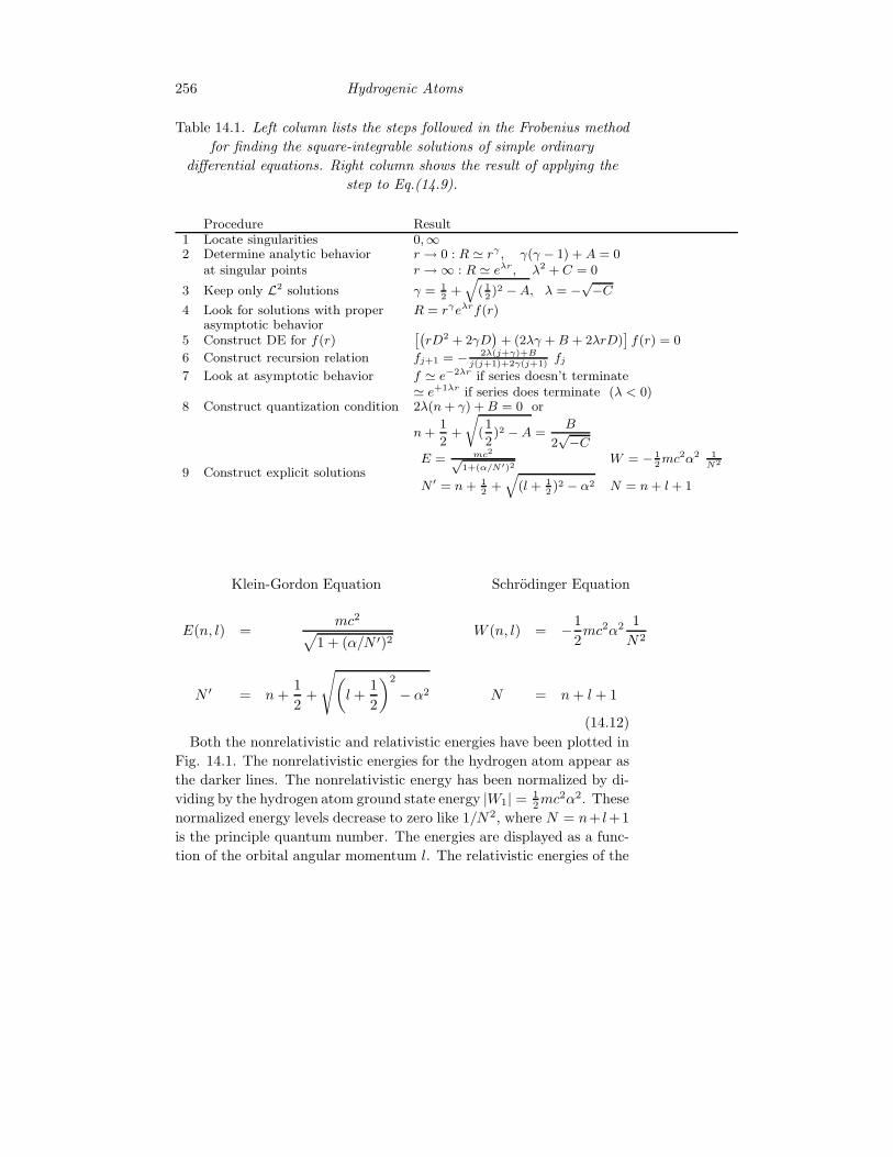
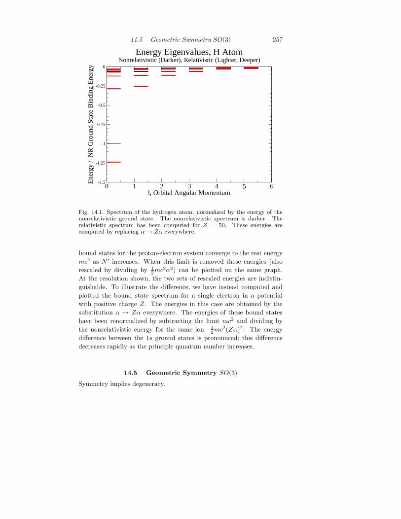
Both the nonrelativistic and relativistic energies have been plotted in
Fig. 14.1. The nonrelativistic energies for the hydrogen atom appear as
the darker lines. The nonrelativistic energy has been normalized by di-
viding by the hydrogen atom ground state energy |W1| = 12mc
2α2. These
normalized energy levels decrease to zero like 1/N2, where N = n+ l+1
is the principle quantum number. The energies are displayed as a func-
tion of the orbital angular momentum l. The relativistic energies of the
14.5 Geometric Symmetry SO(3) 257
0 1 2 3 4 5 6l, Orbital Angular Momentum
-1.5
-1.25
-1
-0.75
-0.5
-0.25
0
Ene
rgy
/ N
R G
roun
d St
ate
Bin
ding
Ene
rgy
Energy Eigenvalues, H AtomNonrelativistic (Darker), Relativistic (Lighter, Deeper)
Fig. 14.1. Spectrum of the hydrogen atom, normalized by the energy of thenonrelativistic ground state. The nonrelativistic spectrum is darker. Therelativistic spectrum has been computed for Z = 50. These energies arecomputed by replacing α → Zα everywhere.
bound states for the proton-electron system converge to the rest energy
mc2 as N ′ increases. When this limit is removed these energies (also
rescaled by dividing by 12mc
2α2) can be plotted on the same graph.
At the resolution shown, the two sets of rescaled energies are indistin-
guishable. To illustrate the difference, we have instead computed and
plotted the bound state spectrum for a single electron in a potential
with positive charge Z. The energies in this case are obtained by the
substitution α → Zα everywhere. The energies of these bound states
have been renormalized by subtracting the limit mc2 and dividing by
the nonrelativistic energy for the same ion: 12mc
2(Zα)2. The energy
difference between the 1s ground states is pronounced; this difference
decreases rapidly as the principle qunatum number increases.
14.5 Geometric Symmetry SO(3)
Symmetry implies degeneracy.

258 Hydrogenic Atoms
To see this, assume gi ∈ G are group operations that leave a hamilto-
nian H invariant (unchanged in form)
giHg−1i = H or giH = Hgi (14.13)
When G is a group of geometric transformations the physical interpre-
tation of this equation is as follows. The hamiltonian H has the same
form in two coordinate systems that differ by the group operation gi.
Under this condition, if |ψ〉 is an eigenstate of H with eigenvalue E, then
gi|ψ〉 is also an eigenstate of H with the same energy eigenvalue E. The
demonstration is straightforward:
H(gi|ψ〉) = (Hgi)|ψ〉 = (giH)|ψ〉 = gi(H |ψ〉) = gi(E|ψ〉) = E(gi|ψ〉)(14.14)
To illustrate this idea, assume that |ψ〉 = ψ2pz (x). A rotation by π/2
radians about the y-axis maps this state to ψ2px(x) and a rotation by
π/2 radians about the x-axis maps this state to −ψ2py(x). By invari-
ance (of the hamiltonian) under the rotation group and the Principle of
Equivalence, these new functions describe possible states of the system,
and these states must exist.
The rotation group O(3) leaves the hamiltonian of the hydrogen atom
invariant in both the nonrelativistic and relativistic cases. In the nonrel-
ativistic case, H = p·p2m − e2
r . The scalar p · p = −~2∇2 is invariant under
rotations, as is also the potential energy term −e2/r. Rotation opera-
tors can be expressed in terms of the infinitesimal generators of rotations
about axis i: ǫijkxj∂k. These geometric operators are proportional to the
physical angular momentum operators Li = (r × p)i = (~/i)ǫijkxj∂k.
Finite rotations can be expressed as exponentials as follows:
R(θ) = eǫijkθixj∂k = eiθ·L/~ (14.15)
The angular momentum operators L = r × p share the same commuta-
tion relations as the infinitesimal generators of rotations r ×∇, up to
the proportionality factor ~/i. The commutation relations are
[Li, Lj ] = i~ǫijkLk (14.16)
It is useful to construct linear combinations of these operators that have
canonical commutation relations of the type described in Chapter 10.

14.5 Geometric Symmetry SO(3) 259
To this end we define the raising (L+) and lowering (L−) operators by
L± = Lx ± iLy. The commutation relations are
[Lz, L±] = ±~L± (14.17)
[L+, L−] = 2~Lz (14.18)
These angular momentum operators are related to the two boson op-
erators as follows: Lz = ~12 (a†1a1 − a†2a2) L+ = ~a†1a2, L− = ~a†2a1.
As a result, the angular momentum operators have matrix represen-
tations with basis vectors | n1 n2 〉 = | j
m〉, with n1 = 0, 1, 2, . . . ,
n2 = 0, 1, 2, . . . , n1 + n2 = 2j, n1 − n2 = 2m, −j ≤ m ≤ +j. These
basis vectors describe the finite dimensional irreducible representations
of the covering group SU(2) of SO(3). The subset of representations
with j = l (integer) describes representations of SO(3).
To see this we construct a coordinate representation of the angular
momentum operators. In spherical coordinates ((x, y, z) → (r, θ, φ) with
x = r sin θ cosφ) these operators are
Lz =~
i
∂
∂φ
L± = ~
(
± ∂
∂θ+ i
cos θ
sin θ
∂
∂φ
) (14.19)
The functions on R3 that transform under the angular momentum op-
erators can be constructed from the mixed basis argument:
〈θφ|L−|l
m〉
↓ ↓
〈θφ|L−|θ′φ′〉 〈θ′φ′|l
m〉 = 〈θφ| l′
m′ 〉 〈 l′
m′ |L−|l
m〉
(14.20)
As usual, the intermediate arguments (with primes) are dummy argu-
ments that are summed or integrated over. The symbols in Eq.(14.20)
have the following meaning
260 Hydrogenic Atoms
〈θφ|L−|θ′φ′〉 Matrix element of the angular momentum shift down oper-
ator in the coordinate representation: ~
(
− ∂∂θ + i cos θ
sin θ∂
∂φ
)
δ(cos θ′ − cos θ)δ(φ′ − φ).
〈 l′
m′ |L−|l
m〉 Matrix element of the angular momentum shift down oper-
ator in the algebraic representation: ~√
(l′ −m′)(l +m)
δl′l δm′,m−1.
〈θφ| l
m〉 Matrix element of the similarity transformation between the
coordinate representation and algebraic representation. Also
called spherical harmonic: Y lm(θ, φ).
This relation can be used to show that there are no geometric functions
associated with values of the quantum number j that are half integral.
It can also be used to constuct the extremal function Y l−l(θ, φ) by solving
the equation L−Yl−l(θ, φ) = 0 in the coordinate representation (Problem
14.12). Finally, the action of the shift up operators can be used to
constuct the remaining functions Y lm(θ, φ) through the recursion relation
involving both the coordinate and the algebraic representations of the
shift up operator L+
L+Ylm(θ, φ) = Y l
m+1(θ, φ)√
(l −m)(l +m+ 1) (14.21)
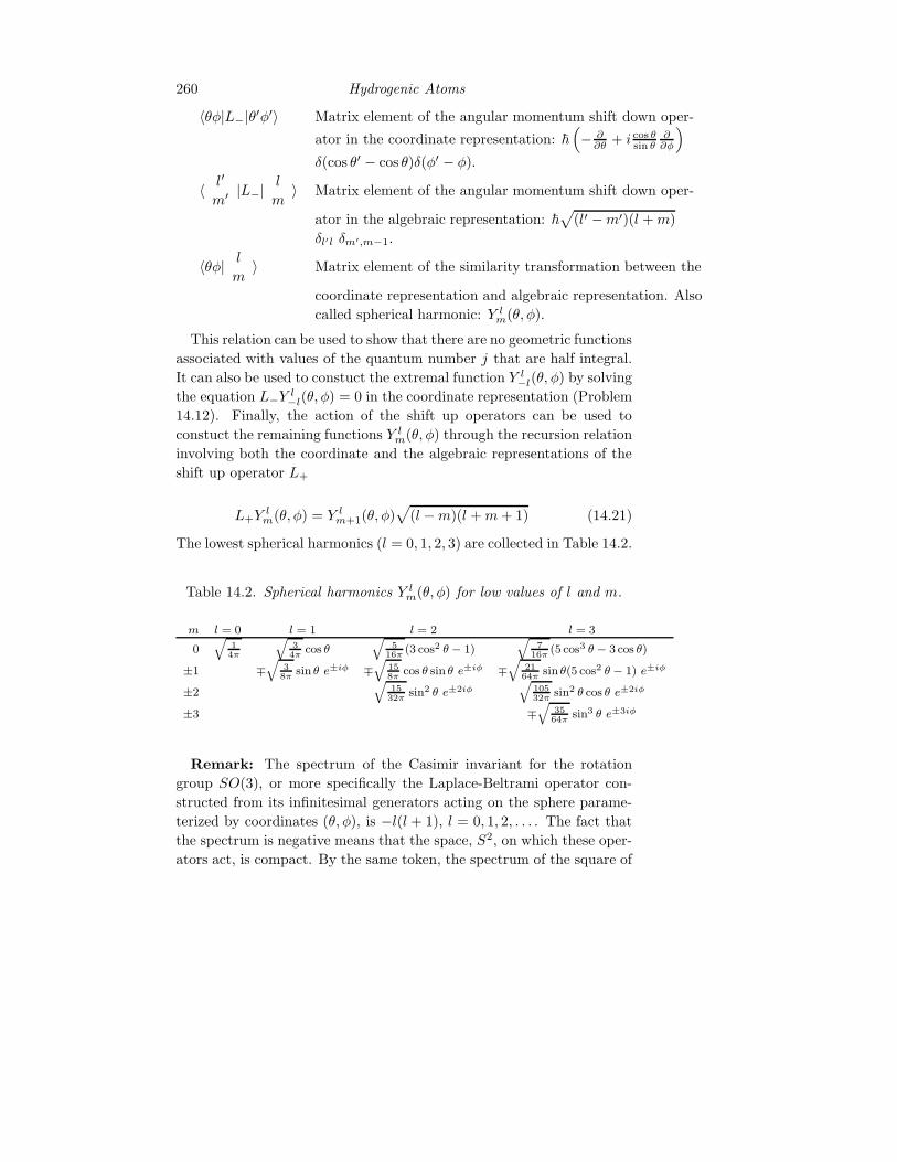
The lowest spherical harmonics (l = 0, 1, 2, 3) are collected in Table 14.2.
Table 14.2. Spherical harmonics Y lm(θ, φ) for low values of l and m.
m l = 0 l = 1 l = 2 l = 3
0q
14π
q
34π
cos θ
q
516π
(3 cos2 θ − 1)q
716π
(5 cos3 θ − 3 cos θ)
±1 ∓
q
38π
sin θ e±iφ ∓
q
158π
cos θ sin θ e±iφ ∓
q
2164π
sin θ(5 cos2 θ − 1) e±iφ
±2q
1532π
sin2 θ e±2iφq
10532π
sin2 θ cos θ e±2iφ
±3 ∓
q
3564π
sin3 θ e±3iφ
Remark: The spectrum of the Casimir invariant for the rotation
group SO(3), or more specifically the Laplace-Beltrami operator con-
structed from its infinitesimal generators acting on the sphere parame-
terized by coordinates (θ, φ), is −l(l + 1), l = 0, 1, 2, . . . . The fact that
the spectrum is negative means that the space, S2, on which these oper-
ators act, is compact. By the same token, the spectrum of the square of

14.6 Dynamical Symmetry SO(4) 261
the angular momentum operator, L · L, is ~2l(l+ 1). This means phys-
ically that the inner product of the angular momentum operator with
itself is never negative, and is quantized by integer angular momentum
values, measured in units of Planck’s constant ~.
14.6 Dynamical Symmetry SO(4)
Symmetry implies degeneracy.
The greater the symmetry, the greater the degeneracy.
The states of the nonrelativistic hydrogen atom with fixed principal
quantum number N = n + l + 1 are degenerate, with energy EN =
− 12mc
2α2 1N2 . There are
∑l=N−1l=0 (2l + 1) = N2 states with this energy.
ThisN2-fold degeneracy is larger than the 2l+1-fold degeneracy required
by rotational invariance of the hamiltonian. If we believe the converse,
that degeneracy implies symmetry, then we might be led to expect that
the hydrogen atom exhibits more symmetry than meets the eye.
In fact this symmetry, called a dynamical symmetry [61], exists and
is related to a constant of motion that is peculiar to 1/r2 force laws.
This constant of motion is known as the Laplace-Runge-Lenz vector.
It is a constant of unperturbed planetary motion, for which the force
law has the form dpdt = −K r
r3 , where K = GMm, G is the universal
gravitational constant, M and m are the two attracting masses, and
r = xi + yj + zk is the vector from one mass to the other. The time
derivative of the vector p × L is
d
dt(p× L) =
dp
dt×L + p×dL
dt↓ ↓
= −K r
r3×(r × m r) + 0
= −mK r(r · r) − r(r · r)r3
= mKd
dt
(r
r
)
(14.22)
In going from the first line in Eq. (14.22) to the second, we use the
fact that L is a constant of motion in any spherically symmetric poten-
tial. We also use the force law for a 1/r potential. In going from the
second line to the third, we express the cross product r × L in terms
of (generally) nonparallel vectors r and r. We also use the identityddt
rr = r/r − (r · r) r/r3. The result is that the Laplace-Runge-Lenz
vector M is a constant of motion: dM/dt = 0, where

262 Hydrogenic Atoms
M =p× L
m−K
r
r(14.23)
In the transition from classical to quantum mechanics the operator
obtained from the classical operator in Eq. (14.23) is not hermitian.
Pauli [56] symmetrized it properly, defining the hermitian quantum me-
chanical operator
M =p× L − L × p
2m−K
r
r(14.24)
where the ˆ over the classical symbol indicates a quantum mechanical
operator. We will dispense with the ˆ over operators, in part to sim-
plify notation, in part to prevent uncertainties in interpretation of the
operator r.
The hermitian operator M in Eq. (14.23) is a constant of motion, as
it commutes with the nonrelativistic hamiltonian: [H,M] = 0. The six
operators Li,Mj obey the following commutation relations
[Li, Lj] = i~ǫijk Lk
[Li,Mj] = i~ǫijk Mk
[Mi,Mj] =
(
−2H
m
)
i~ǫijk Lk
(14.25)
These are the commutation relations for the Lie algebra of the group
SO(4) for bound states (E < 0) or SO(3, 1) for excited states (E > 0).
The operators L and M also obey
L ·M = M · L = 0
M · M =2H
m
(
L · L + ~2)
+K2
(14.26)
In order to simplify the discussion to follow, and make this discus-
sion as independent of the principal quantum number N as possible, we
renormalize the Laplace-Runge-Lenz vector by a scale factor as follows:
M′ =(
− m2H
)1/2M. (For E > 0 change − → + and SO(4) → SO(3, 1).)
The commutation relations of these operators are now
[Li, Lj ] = i~ǫijk Lk[
Li,M′j
]
= i~ǫijk M′k
[
M ′i ,M
′j
]
= i~ǫijk Lk
(14.27)

14.6 Dynamical Symmetry SO(4) 263
The Lie algebra so(4) is the direct sum of two Lie algebras of type
so(3) (cf. Figs. 10.3, 10.8(b)). It is useful to introduce two vector
operators A and B as follows
A = 12 (L + M′)
B = 12 (L − M′)
(14.28)
The operators A and B have angular momentum commutation relations.
Further, they mutually commute. Finally, their squares have the same
spectrum.
It is useful at this point to introduce the Schwinger representation for
the angular momentum operators A in terms of two independent boson
modes: A3 = 12 (a†1a1 − a†2a2), A+ = a†1a2, A− = a†2a1 (for simplicity, set
~ → 1). A similar representation of the angular momentum operators
B in terms of two independent boson operators b1, b2 and their creation
operators is also introduced.
Basis states for a representation of the algebra spanned by the op-
erators A have the form |p1, p2〉, with p1 + p2 = 2ja constant and
p1 − p2 = ma. The 2ja + 1 basis states correspond to p1 = 2ja, p2 = 0;
p1 = 2ja − 1, p2 = 1; etc. For B the basis states are |q1, q2〉, with
q1 + q2 = 2jb constant and q1 − q2 = mb. The invariant operators are
A · A = ja(ja+1) and B · B = jb(jb+1). Since A ·A = B ·B (cf. Prob-
lem 14.15), ja = jb and the set of states related by the shift operators is
(2j + 1)2 fold degenerate, where 2j + 1 = N = n+ l+ 1.
States with good l and m quantum numbers can be constructed from
these states using Clebsch-Gordon coefficients:
| l
m〉 = | j/2 j/2
ma mb〉〈 j/2 j/2
ma mb| l
m〉 (14.29)
The action of the Laplace-Runge-Lenz shift operators on these states,
and the spherical harmonics, is determined in a straightforward way.
For example, M ′+ = A+ −B+ = a†1a2 − b†1b2, so that
M ′+Y
lm = 〈θφ|
(
| j/2 j/2
ma + 1 mb〉〈 j/2 j/2
ma mb| l
m〉 ×
√
(j/2 −ma)(j/2 +ma + 1) −
| j/2 j/2
ma mb + 1〉〈 j/2 j/2
ma mb| l
m〉 ×
√
(j/2 −mb)(j/2 +mb + 1)
)
(14.30)

264 Hydrogenic Atoms
In general, the Laplace-Runge-Lenz operators shift the values of l and
m by ±1 or 0, while the angular momentum shift operators change
only m by ±1. However, for certain stretched values of the Clebsch-
Gordon coefficients, the Laplace-Runge-Lenz vectors act more simply,
for example [15]
M ′z|N
l
±l 〉 = D1|Nl + 1
±l 〉 D1 =1
N
√
N2 − (l + 1)2
2l+ 3
M ′±|N
l
±l 〉 = ±D2|Nl + 1
±(l + 1)〉 D2 =
1
N
√
2l+ 2
2l+ 3[N2 − (l + 1)2]
(14.31)
14.7 Relation With Dynamics in Four Dimensions
The operators L and M′ are infinitesimal generators for the orthogonal
group SO(4). The relation between motion in the presence of a Coulomb
or gravitational potential and motion in four (mathematical) dimensions
was clarified by Fock [19]. Motion of a particle in a 1/r potential is
equivalent to motion of a free particle in the sphere S3 ⊂ R4.
It is useful first to establish an orthogonal coordinate system in R3.
It is natural to do this in terms of the constant physical vectors that
are available. These include the vectors L and M. Their cross product
W = L × M is orthogonal to both and also a constant of motion. These
classical vectors obey:
L = r × p L · L = L2
M =p × L
m−K
r
rM ·M = M2 =
2E
mL2 +K2
W =p
mL2 −K
L × r
rW · W = L2M2
(14.32)
The particle moves in a plane perpendicular to the angular momentum
vector L, since r · L = 0. The momentum vector moves in the same
plane, since p · L = 0. While r moves in an ellipse, the momentum vector
moves on a circle. For simplicity we choose the z axis in the direction of
L and the x- and y-axes in the directions of M and W. In this coordinate
system pz = 0, px = p ·M/√
M · M and py = p ·W/√
W · W. The
two nonzero components of the momentum vector are not independent,

14.7 Relation With Dynamics in Four Dimensions 265
but obey the constraint
p2x +
(
py − mM
L
)2
=
(
mK
L
)2
(14.33)
This is the equation of a circle in the plane containing the motion. As
the particle moves in the plane of motion on an elliptical orbit with
one focus at the source, its momentum moves in the same plane on a
circular orbit (radius mK/L) with the center displaced from the origin
by mM/L.
The circle in R3 is lifted to a circle in S3 ⊂ R4 by a projective trans-
formation. We extend coordinates from R3 to R4 as follows:
(x, y, z) ∈ R3 → (w, x, y, z) ∈ R4
(px, py, pz) ∈ R3 → (pw, px, py, pz) ∈ R4 (14.34)
With p0 =√
−2E/m, define the unit vector u ∈ S3 ⊂ R4 by the
projective transformation T :
uT=
p · p− p20
p · p + p20
w +2p0
p · p + p20
p (14.35)
Here w is a unit vector in R4 that is orthogonal to all vectors in the
physical space R3. The transformation in [Eq.(14.35)] is a stereographic
projection. It is invertible and preserves angles (conformal). It is a sim-
ple matter to check that u is a unit vector. The circular trajectory in R3
[Eq.(14.33)] lifts to a circle in S3. Reversibly, circles in S3 project down
to circles in the physical R3 space under the reverse transformation.
Rotations in SO(4) rigidly rotate the sphere S3 into itself. They
rotate circles into circles, which then project down to circular momentum
trajectories in the physical space R3:
circle in R3 T−→ circle in S3 SO(4)−→ circle in S3 T−1
−→ circle in R3 (14.36)
The subgroup SO(3) of rotations around the w axis acts only the the
physical space R3. In this subgroup, the subgroup SO(2) of rotations
around the L axis leaves L fixed and simply rotates M in the plane
of motion. The coset representatives SO(3)/SO(2) act to reorient the
plane of motion by rotating the angular momentum vector L while keep-
ing the magnitude of M fixed. Rotations in the coset SO(4)/SO(3) act
to change the lengths of both L and M. All group operations in SO(4)
keep p0 fixed. In this way the group SO(4) maps states with principal
quantum number N into (linear combinations of) states with the same

266 Hydrogenic Atoms
principal quantum number N . In short, SO(4) acts on the bound hydro-
gen atom states through unitary irreducible representations of dimension
N2 = (n+ l + 1)2.
14.8 DeSitter Symmetry SO(4, 1)
The dynamical symmetry group SO(4) that rotates bound states to
bound states does not change their energy; the dynamical symmetry
group SO(3, 1) that rotates scattering states to scattering states does
not change their energy either. It would be nice to find a set of trans-
formations that rescales the energy. If such a group could be found,
it would be possible, for example, to map the 1s ground state into
any other bound state. Such a group exists: it is the deSitter group
SO(4, 1) [51, 54].
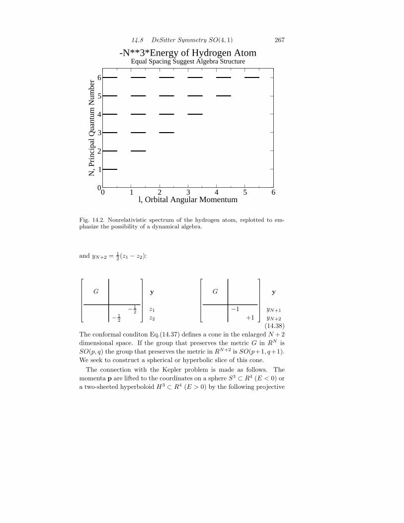
That such a group might exist is strongly suggested by the appear-
ance of the hydrogen atom spectrum, as replotted in Fig. 14.2. In
this figure we have multiplied each energy eigenvalue by −N3, where
N is the principle quantum number. The rescaled energies have been
plotted as a function of N (vertically) and orbital angular momentum
quantum number l (horizontally). In this format, the ewigenvalue spec-
trum bears a strong resemblance to the spectrum of states that supports
finite-dimensional representations of su(2) (Fig. 6.1) and the infinite-
dimensional representations of su(1, 1) (Fig. 11.2).
We begin with a group that preserves inner products in some N -
dimensional linear vector space: x′ = Mx, with M a transformation in
the group and the inner product defined by (x,x)N = xtgx = xigijxj .
As always, the metric-preserving condition leads to M tGM = G.
It is useful to define a newN -vector y as a scaled version of the original
vector: y = λx. We introduce two additional coordinates by defining
z1 = λ and z2 = λ(x,x)N . With these definitions we find the conformal
condition
(y,y)N − z1z2 = (λx, λx)N − λ [λ(λx, λx)N ] = 0 (14.37)
The conformal condition defines an inner product in the N + 2 dimen-
sional linear vector space that is nondiagonal in the coordinates y, z1, z2but diagonal in the coordinates y, yN+1, yN+2, with yN+1 = 1
2 (z1 + z2)
14.8 DeSitter Symmetry SO(4, 1) 267
0 1 2 3 4 5 6l, Orbital Angular Momentum
0
1
2
3
4
5
6
N, P
rinc
ipal
Qua
ntum
Num
ber
-N**3*Energy of Hydrogen AtomEqual Spacing Suggest Algebra Structure
Fig. 14.2. Nonrelativistic spectrum of the hydrogen atom, replotted to em-phasize the possibility of a dynamical algebra.
and yN+2 = 12 (z1 − z2):
G
− 12
− 12
y
z1z2
G
−1
+1
y
yN+1
yN+2
(14.38)
The conformal conditon Eq.(14.37) defines a cone in the enlarged N + 2
dimensional space. If the group that preserves the metric G in RN is
SO(p, q) the group that preserves the metric in RN+2 is SO(p+1, q+1).
We seek to construct a spherical or hyperbolic slice of this cone.
The connection with the Kepler problem is made as follows. The
momenta p are lifted to the coordinates on a sphere S3 ⊂ R4 (E < 0) or
a two-sheeted hyperboloid H3 ⊂ R4 (E > 0) by the following projective

268 Hydrogenic Atoms
transformations:
u =12 (p2
0 − p · p)12 (p2
0 + p · p)w +
p0p12 (p2
0 + p · p)E < 0
u =12 (p2
0 + p · p)12 (p2
0 − p · p)w +
p0p12 (p2
0 − p · p)E > 0
(14.39)
For the 4-vectors u the metricG that appears in Eq.(14.38) is determined
from the denominators in Eq.(14.39):
utGu = u20 ±
3∑
i=1
u2i
+ for E < 0
− for E > 0(14.40)
The algebraic surfaces on which the projective vector u lies is defined
by the condition utGu = 1.
The connection with the conformal transformations introduced above
is as follows. The group that leaves invariant the conformal metric diag
(1,±I3,−1,+1) is SO(5, 1) for E < 0 and SO(2, 4) for E > 0. On
the surfaces (sphere, hyperboloid) the condition utGu = 1 is satisfied,
so that z1 = z2, y4 = λ and y5 = 0 (the six coordinates are labeled
(y0,y = λu, y4 = 12 (z1 + z2), y5 = 1
2 (z1 − z2)). Transformations that
map the algebraic surface to itself must map y5 = 0 to y5 = 0. It is
a simple matter to verify that this is the matrix subgroup of the 6 × 6
matrix group SO(5, 1) or SO(2, 4) of the form
[
M 0
0 1
]
, with M a
5 × 5 matrix that preserves the metric diag (1,±I3,−1) in R5. This is
SO(4, 1) for E < 0 and SO(1, 4) for E > 0.
It remains to show that this group maps these algebraic surfaces into
themselves. To this end we write the linear transformation in R5 as
follows[
λu
λ
]′
=
[
A B
C D
] [
λu
λ
]
(14.41)
where A is a 4 × 4 matrix, etc. From this we determine
u′ =A(λu) +Bλ
C(λu) +Dλ(14.42)
The inner product of u′ with itself satisfies
(u′)tGu′−1 =(Aλu +Bλ)tG(Aλu +Bλ) − (Cλu +Dλ)t(Cλu +Dλ)
(Cλu +Dλ)t(Cλu +Dλ)(14.43)

14.8 DeSitter Symmetry SO(4, 1) 269
By using the relations among the submatrices required by the metric
preserving condition (e.g., AtGA−CtC = G, etc.) it is a simple matter
to show that this reduces to
(u′,u′)N − 1 =(u,u)N − 1
(Cu +D)t(Cu +D)(14.44)
In short, the algebraic surface is invariant under this transformation
group.
Remark: The subgroup SO(4) rigidly rotates the sphere S3 ⊂ R4
into itself while the subgroup SO(3, 1) “rigidly rotates” the hyperboloid
into itself. In the latter case this is less intuitive. This means that the
coordinates of the hyperboloid are mapped into themselves by a linear
transformation in R4. The group SO(4, 1) maps coordinates in these
spaces to themselves through a nonlinear transformation in R4: in this
case a simple projective transformation. It is a linear transformation in
R5.
The infinitesimal generators of this nonlinear transformation are con-
structed as follows [3, 4]. For E < 0 introduce a 4-vector u as usual
(u0 → u4)
u = 2p4(p · p + p24)
−1p
u4 = (p · p− p24)(p · p + p2
4)−1 (14.45)
Define the 4-vector B in terms of the 4-vector u and the angular mo-
mentum vector L and the scaled (by 1/√
2m|E|) Runge-Lenz vector M′
as follows:
B = M′u4 + L × u− 32 iu = i
2
[
u,L2 + M′2]
B4 = M′ · u + 32 iu = i
2
[
u4,L2 + M′2
]
The operatorsLi, M′i , andBµ are the infinitesimal generators of SO(4, 1)
as follows, for E < 0.
0 L3 −L2 M1 B1
−L3 0 L1 M2 B2
L2 −L1 0 M3 B3
−M1 −M2 −M3 0 B4
B1 B2 B3 B4 0
+
+
+
+
−
270 Hydrogenic Atoms
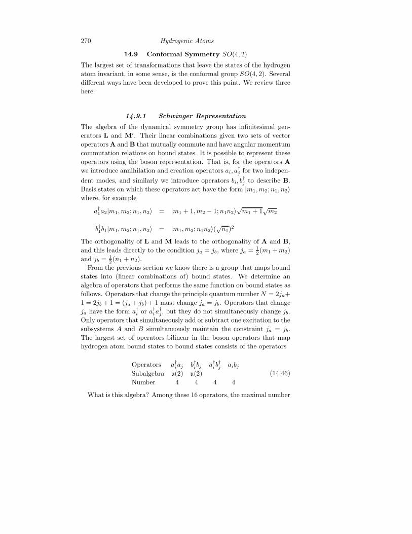
14.9 Conformal Symmetry SO(4, 2)
The largest set of transformations that leave the states of the hydrogen
atom invariant, in some sense, is the conformal group SO(4, 2). Several
different ways have been developed to prove this point. We review three
here.
14.9.1 Schwinger Representation
The algebra of the dynamical symmetry group has infinitesimal gen-
erators L and M′. Their linear combinations given two sets of vector
operators A and B that mutually commute and have angular momentum
commutation relations on bound states. It is possible to represent these
operators using the boson representation. That is, for the operators A
we introduce annihilation and creation operators ai, a†j for two indepen-
dent modes, and similarly we introduce operators bi, b†j to describe B.
Basis states on which these operators act have the form |m1,m2;n1, n2〉where, for example
a†1a2|m1,m2;n1, n2〉 = |m1 + 1,m2 − 1;n1n2〉√m1 + 1
√m2
b†1b1|m1,m2;n1, n2〉 = |m1,m2;n1n2〉(√n1)
2
The orthogonality of L and M leads to the orthogonality of A and B,
and this leads directly to the condition ja = jb, where ja = 12 (m1 +m2)
and jb = 12 (n1 + n2).
From the previous section we know there is a group that maps bound
states into (linear combinations of) bound states. We determine an
algebra of operators that performs the same function on bound states as
follows. Operators that change the principle quantum numberN = 2ja+
1 = 2jb + 1 = (ja + jb) + 1 must change ja = jb. Operators that change
ja have the form a†i or a†ia†j, but they do not simultaneously change jb.
Only operators that simultaneously add or subtract one excitation to the
subsystems A and B simultaneously maintain the constraint ja = jb.
The largest set of operators bilinear in the boson operators that map
hydrogen atom bound states to bound states consists of the operators
Operators a†iaj b†ibj a†ib†j aibj
Subalgebra u(2) u(2)
Number 4 4 4 4
(14.46)
What is this algebra? Among these 16 operators, the maximal number

14.9 Conformal Symmetry SO(4, 2) 271
of mutually commuting operators that can be found is four. These are
conveniently chosen as the number operators for the four boson modes:
(H1, H2, H3, H4) = (a†1a1, a†2a2, b
†1b1, b
†2b2). The remaining twelve oper-
ators have eigenoperator commutation relations with this set:
a†1a2 (+1,−1, 0, 0) a†1b†1 (+1, 0,+1, 0) a1b1 (−1, 0,−1, 0)
a†2a1 (−1,+1, 0, 0) a†1b†2 (+1, 0, 0,+1) a1b2 (−1, 0, 0,−1)
b†1b2 (0, 0 + 1,−1) a†2b†1 (0,+1,+1, 0) a2b1 (0,−1,−1, 0)
b†2b1 (0, 0,−1,+1) a†2b†2 (0,+1, 0,+1) a2b2 (0,−1, 0,−1)
(14.47)
All these roots have equal length, and inner products among these roots
are all ± 12 or 0. The operator
(a†1a1 + a†2a2) − (b†1b1 + b†2b2)
commutes with all operators in this set. It is a constant of motion, and
in fact vanishes on all hydrogen atom bound states. As a result the
algebra is the direct sum of an abelian invariant subalgebra spanned by
this operator, and a rank-three simple Lie algebra, all of whose roots
have equal lengths and are either orthogonal or make angles of π4 or 3π
4
radians with each other. The algebra is uniquely a real form of A3 = D3.
Which real form? It is possible to form a number of subalgebras of
type A1 from these operators:
a†1a2 a†2a112 (a†1a1 − a†2a2) su(2)
b†1b2 b†2b112 (b†1b1 − b†2b2) su(2)
a†ib†j aibj
12 (a†iai + b†jbj + 1) su(1, 1)
The first two are compact, the last four are not compact. The maximal
compact subalgebra is spanned by the two compact subalgebras together
with the diagonal operator a†1a1 +a†2a2 + b†1b1 + b†2b2. This is the algebra
so(4)+so(2). The fifteen dimensional Lie algebra that maps bound states
to bound states is therefore so(4, 2) = su(2, 2). This is the conformal
algebra.
14.9.2 Dynamical Mappings
Although the classical Kepler problem is analytically solvable, analyt-
icity disappears under perturbation. In this case classical orbits must
be computed numerically. At points of very close approach the veloc-
ity of the particles increases greatly, so it is prudent to slow down the

272 Hydrogenic Atoms
integration time step to preserve accuracy. This procedure has been im-
plemented formally through a canonical transformation [48, 67], and is
now widely known as the Kustaanheimo-Stiefel transformation. Under
this transformation time is stretched out when the distance R between
the interacting particles becomes small. In addition the (relative) co-
ordinates are projected from R3 to a fictitious space R4. Under this
transformation, and a constraint, the Kepler hamiltonian is transformed
into a four dimensional harmonic oscillator hamiltonian.
Coordinates (q1, q2, q3, q4) in the fictitions space R4 are related to
coordinates (Q1, Q2, Q3) in the real space by the 4 × 4 transformation
Q1
Q2
Q3
Q4
= MKS
q1q2q3q4
=
q1 −q2 −q3 q4q2 q1 −q4 −q3q3 q4 q1 q2q4 −q3 q2 −q1
q1q2q3q4
(14.48)
The transformation is constructed so that the “fourth” real coordinate
Q4 is identically zero. This transformation is invertible provided q21 +
q22 + q23 + q24 6= 0. The distance R =√
Q21 +Q2
2 +Q23 in R3 and the
distance q =√
q21 + q22 + q23 + q24 in R4 are related by: R = q2.
The other half of the canonical transformation, involving the momenta
in the real and fictitious spaces, is
(P1, P2, P3, P4)t =
1
2RMKS(p1, p2, p3, p4)
t
A constraint condition must be applied to force P4 = 0. This condition
is
ζ = −2RP4 = (q1p4 − q4p1) + (q3p2 − q2p3) = 0 (14.49)
With this constraint we find P 2 = P 21 + P 2
2 + P 23 = 1
4Rp2 − ζ2
4R2 →1
4R (p21 + p2
2 + p23 + p2
4). With these transformations the hamiltonian in
the real space can be transformed to a hamiltonian in the fictitious space
by
P 2
2m− e2
R= E
×R−→ R P 2
2m− e2 = E R
KS−→ p2
8m− e2 = E q2 (14.50)
This is the hamiltonian for a four-dimensional harmonic oscillator when
E < 0, as easily seen by rearranging the terms
p2
2m− 4Eq2 = 4e2 (14.51)

14.9 Conformal Symmetry SO(4, 2) 273
The angular momentum operators in the real and fictitious spaces are
bilinear products of the position and momentum coordinates, as follows:
(Q1, Q2, Q3, Q4)
0 θ3 −θ2 ∗−θ3 0 θ1 ∗θ2 −θ1 0 ∗−∗ −∗ −∗ 0
P1
P2
P3
P4
1
2(q1, q2, q3, q4)
0 θ3 −θ2 θ1−θ3 0 θ1 θ2θ2 −θ1 0 θ3−θ1 −θ2 −θ3 0
p1
p2
p3
p4
(14.52)
Similar expressions can be given for the Runge-Lenz vector. However,
these are quadratic in the position and momentum operators. As a result
they must be expressed in matrix form using 8 × 8 matrices acting on
the vector (q1, q2, q3, q4; p1, p2, p3, p4) on the left and its transpose on the
right [59].
We now ask: what is the largest group of transformations on the
coordinates and momenta that:
a. is linear
b. is canonical
c. preserves ζ = 0.
We address this question in the usual way. Linear transformations al-
low us to use matrices. These are 8 × 8 matrices acting on the four
coordinates and four momenta. Preserving the Poisson brackets re-
quires that the matrices satisfy a symplectic metric-preserving condition:
M tG1M = G1. Preserving the condition ζ = 0 requires these transfor-
mations to satisfy another metric-preserving condition: M tG2M = G2.
The matrices Gi have the form Gi =
[
0 Mi
−Mi 0
]
, where
M1 =
1 0 0 0
0 1 0 0
0 0 1 0
0 0 0 1
M2 =
0 0 0 1
0 0 −1 0
0 1 0 0
−1 0 0 0
M t1 = +M1 Gt
1 = −G1 M t2 = −M2 Gt
2 = +G2
(14.53)
The metric G1 is antisymmetric and the metric G2 is symmetric, with

274 Hydrogenic Atoms
signature (+4,−4). The group that preserves the antisymmetric met-
ric is Sp(8;R) and the group that preserves the symmetric metric is
SO(4, 4). The group that satisfies both metric-preserving conditions is
their intersection:
Sp(8;R) ∩ SO(4, 4) = SU(2, 2) ≃ SO(4, 2) (14.54)
The simplest way to see this result is to perform a canonical transfor-
mations from coordinates (q, p) to coordinates (s, r):
[
s1r4
]
= 1√2
[
1 1
−1 1
] [
q1p4
] [
s2r3
]
= 1√2
[
−1 1
−1 −1
] [
q2p3
]
[
s3r2
]
= 1√2
[
1 1
−1 1
] [
q3p2
] [
s4r1
]
= 1√2
[
−1 1
−1 −1
] [
q4p1
]
(14.55)
Since the new coordinates are already canonical, only the condition ζ = 0
remains to be satisfied. It is a simple matter to verify that
z1 = 1√2(s1 + is2) z2 = 1√
2(r1 + ir2)
z∗1z1 − z∗2z2 + z∗3z3 − z∗4z4 = ζ
z3 = 1√2(s3 + is4) z4 = 1√
2(r3 + ir4)
(14.56)
The noncompact group U(2, 2) preserves the constraint Eq.(14.49).
14.9.3 Lie Algebra of Physical Operators
A number of workers have shown that the Hamiltonian describing the
interaction of a charged particle interacting with an external Coulomb
field [V (r) = −e2/r] can be expressed in terms of operators that close
under commutation. The Lie algebra that these operators span is iso-
morphic with the Lie algebra of a noncompact orthogonal group.
Three vector operators and a scalar operator
J = r × p Angular Momentum
M = 12mp × L − L× p−K r
r Laplace Runge Lenz vector
A = 12mp × L − L× p +K r
r Dual vector
A4 = r · p + 32
~
i Dual scalar(14.57)
close under commutation to span a Lie algebra that is isomorphic with
so(4, 1).

14.10 Spin Angular Momentum 275
Five additional operators can be introduced that extend the algebra to
so(4, 2). These include one vector operator and two additional operators:
Γi = rpi
Γ4 = 12 (rp · p − r)
Γ5 = 12 (rp · p + r)
(14.58)
The commutation relations that these 15 operators satisfy are summa-
rized by the 6 × 6 matrix
0 J3 −J2 M1 A1 Γ1
−J3 0 J1 M2 A2 Γ2
J2 −J1 0 M3 A3 Γ3
−M1 −M2 −M3 0 A4 Γ4
A1 A2 A3 A4 0 Γ5
Γ1 Γ2 Γ3 Γ4 −Γ5 0
+
+
+
+
−−
The four triplets Ji,Mi, Ai,Γi (i = 1, 2, 3) have transformation prop-
erties of three-vectors under rotations. The three additional operators
A4,Γ4,Γ5 close under commutation and span a Lie algebra that is iso-
morphic with so(2, 1).
The Schrodinger and Klein-Gordon Hamiltonians for an electron of
charge −e in the Coulomb field Φ(r) = e/r of a proton can be expressed
in terms of operators of type A4,Γ4, and Γ5. These operators are dis-
played in Table 14.3, along with the Hamiltonians and the algebraic
representation of the wave equations.
14.10 Spin Angular Momentum
The interaction of the electron with the electromagnetic field is properly
described by the Dirac equation. The electromagnetic field (E,B) is
described by the four-vector potential Aµ = (φ,A). The electron has
charge q = −e (where e is the charge on the proton) and spin 12 . The
Dirac equationHDψ = Eψ is a matrix differential equation of first order:
HD = −eφ(r) + βmc2 + γ · (cp + eA) (14.59)
The 4 × 4 matrices β and γi can be chosen as
β =
[
I2 0
0 −I2
]
γi =
[
0 σi
σi 0
]
(14.60)

276 Hydrogenic Atoms
Table 14.3. Nonrelativistic and relativistic Hamiltonians for a spinless
particle, operator representation of the operators A4,Γ4, and Γ5,
expression of the Hamiltonians and wave equations in terms of these
operators, and explicit values of the coefficients in these equations. In
the event a magnetic field B is present, the momentum operators p
should be replaced by π = p − qcA. Under this condition the operators
still close under commutation.
Hp2
2m− α
r
p
p2 + m2 − αr
A4 r · p − i r · p − i
Γ412(rp · p − r)
1
2(rp · p − r − α2
r)
Γ512(rp · p + r)
1
2(rp · p + r − α2
r)
Θ r(HS − W ) r
“
HKG +α
r
”2
−“
E +α
r
”2ff
A(Γ5 + Γ4) + B(Γ5 − Γ4) + C A(Γ5 + Γ4) + B(Γ5 − Γ4) + CA 1/2m 1B −W m2 − E2
C −α −2αE
Here σi are the standard Pauli 2 × 2 spin matrices (cf., Eq. (3.39),
Problem 3.1).
The 15 dimensional Lie algebra for the Dirac equation is spanned by
the operators J,M,A,Γ as given in Eq. (14.57), and the three operators
A4,Γ4,Γ5. The latter two are modified to allow a treatment of the Dirac
operator along the same lines as the treatment of the Schrodinger and
Klein-Gordon operators given in Subsection 14.9.3. We define operators
M4 = r · p − i
Γ4 =1
2
(rp · p− r − α2
r− iαγ · r
r2)
Γ5 =1
2
(rp · p + r − α2
r− iαγ · r
r2
(14.61)
As before, the substitution p → π = p− qcA is in order in the event there
is a nonzero magnetic field B. These operators close under commuta-
tion to form an so(2, 1) Lie algebra. These operators also close under
commutation with the four three-vectors Ji,Mi, Ai,Γi defined in Table
14.3. The Dirac hamiltonian is expressed in terms of these generators
as follows:

14.11 Spectrum Generating Group 277
Θ = r
(
HD +α
r
)2
−(
E +α
r
)2
= A(Γ5 + Γ4) +B(Γ5 − Γ4) + C
(14.62)
where the coefficients A,B,C have exactly the same values as for the
Klein-Gordon operator (cf., Table 14.3). In short, the operators Γ4,Γ5
are modified but the relation among these operators in the algebraic
representation of the relativistic wave equations is not.
14.11 Spectrum Generating Group
The physics of the hydrogenic problem is determined primarily by the
radial equation Eq. (14.9). It is possible to determine solutions of this
equation using operators that close under commutation. These are the
generators of a Lie algebra. The corresponding group is called a spec-
trum generating group.
To construct a set of operators that close under commutation, we first
simplify the radial equation by multiplying on the left by r
(
rD2 +A
r+B + Cr
)
R(r) = 0 (14.63)
with D = d/dr. The operators r and D behave under commutation like
the boson creation and annihilation operators a† and a. In fact, the
nonzero commutation relations are
[rD, r] = +r[
a†a, a†]
= +a†
[
rD, rD2]
= −rD2[
a†a, a†aa]
= −a†aa[
r, rD2]
= −2rD[
a†, a†aa]
= −2a†a
(14.64)
The linear combinations rD2 + r and rD2 − r are compact and non-
compact, respectively. In order to model the differential operator Eq.
(14.63) with a set of operators that close under commutation to form a
finite-dimensional Lie algebra, we must be careful, as

278 Hydrogenic Atoms
[
rD,1
r
]
= −1
r
[
rD2,1
r
]
=2
r2− 1
rD
We choose as operators in the Lie algebra so(2, 1) the three differential
operators
Γ5 =1
2
(
rD2 +a
r− r
)
Γ4 =1
2
(
rD2 +a
r+ r
)
M4 = rD
(14.65)
The Casimir operator for this algebra is C2 = Γ25 −Γ2
4 −M24 = −a. The
representations of this algebra have been described in Problem 11.6.
The radial equation Eq. (14.63) is expressed in terms of the three
operators as follows (a→ A)
((Γ5 + Γ4) +B + C(Γ4 − Γ5))R(r) = 0 (14.66)
Next, we rotate the generators of the algebra according to
eθM4
(
Γ5
Γ4
)
e−θM4 =
[
cosh θ − sinh θ
− sinh θ cosh θ
](
Γ5
Γ4
)
(14.67)
When this similarity transformation is applied to Eq.(14.66) we obtain
the following result:
[(
e−θ − C eθ)
Γ5 +(
e−θ + C eθ)
Γ4 +B]
eθM4R(r) = 0 (14.68)
The rotation angle θ can be chosen to eliminate either the noncompact
generator Γ4 or the compact generator Γ5, depending on the sign of the
parameter C.
14.11.1 Bound States
If C < 0 we can choose e−θ + C eθ = 0, so that the resulting equation
becomes

14.11 Spectrum Generating Group 279
(
2√−C Γ5 +B
)
u(r) = 0 (14.69)
where u(r) = eθM4R(r). If A is the Casimir invariant of this represen-
tation of su(1, 1), the discrete spectrum of the compact operator Γ5 is
N = − 12 +
√
(12 )2 −A+1+n, n = 0, 1, 2, . . . . This result leads directly
to the eigenvalue spectrum for the nonrelativistic and the relativistic
hydrogen atom (no spin) obtained in Eq. (14.12).
Remark: The spectrum generating algebra Eq. (14.65) acts in Hilbert
spaces that carry unitary irreducible representations of the noncompact
group SO(2, 1). These representations are indexed by an integer l that
has an interpretation as angular momentum. The energy spectrum
that we have computed has the behavior (in the nonrelativistic case)
W = − 12mc
2α2 1(N)2 , where N = l+ 1 + k, k = 0, 1, 2, . . . . Here N is the
principle quantum number. The result is that this algebra acts to change
the principle quantum number while keeping l constant. Since the three
operators in the spectrum generating algebra commute with the angular
momentum operators, the quantum number ml (eigenvalue of Lz) is also
invariant under the action of these operators. The states connected by
the operators of this so(2, 1) algebra are |N, lm〉 ↔ |N ± 1, lm〉. The
states on which these operators act are organized in “angular momentum
towers.” These states are organized vertically in Fig 14.2.
Remark: The angular momentum operators Lz, L± act on multiplets
shown as a single horizontal line in Figs. 14.1 and 14.2. The operators
Mz,M± associated with the Laplace-Runge-Lenz vector act horizontally
on the levels shown in these two figures. The operators Γz,Γ± = Γ4 ±iM4 act vertically on the levels shown in these figures. Since [L,Γ] = 0,
the operators Γ do not change the m values of hydrogenic states.
Remark: The shift down operator Γ− annihilates the ground state
in a given angular momentum tower: Γ−〈r|Nl = N − 1
m〉 = 0. Since
the differential operators are known, this relation can be used, as was
the relation L−Ylm=−l(θ, φ) = 0, to determine the radial wavefunction
〈r|N, l = N − 1〉.
14.11.2 Scattering States
If C > 0 we can choose θ so that e−θ −C eθ = 0. Eq. (14.66) reduces to
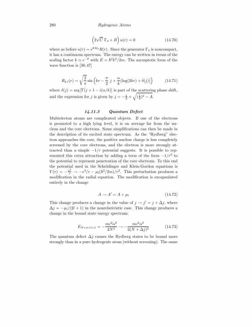
280 Hydrogenic Atoms
(
2√C Γ4 +B
)
u(r) = 0 (14.70)
where as before u(r) = eθM4R(r). Since the generator Γ4 is noncompact,
it has a continuous spectrum. The energy can be written in terms of the
scaling factor k ≃ e−θ with E = ~2k2/2m. The asymptotic form of the
wave function is [38, 47]
Rk,l(r) ∼√
2
πsin
(
kr − π
2j +
α
k(log(2kr) + δ(j))
)
(14.71)
where δ(j) = arg [Γ(j + 1 − i(α/k)] is part of the scattering phase shift,
and the expression for j is given by j = − 12 +
√
(12 )2 −A.
14.11.3 Quantum Defect
Multielecton atoms are complicated objects. If one of the electrons
is promoted to a high lying level, it is on average far from the nu-
cleus and the core electrons. Some simplifications can then be made in
the description of its excited state spectrum. As the “Rydberg” elec-
tron approaches the core, the positive nuclear charge is less completely
screened by the core electrons, and the electron is more strongly at-
tracted than a simple −1/r potential suggests. It is possible to rep-
resented this extra attraction by adding a term of the form −1/r2 to
the potential to represent penetration of the core electrons. To this end
the potential used in the Schrodinger and Klein-Gordon equations is
V (r) = − e2
r → −e2/r − µl(~2/2m)/r2. This perturbation produces a
modification in the radial equation. The modification is encapsulated
entirely in the change
A→ A′ = A+ µl (14.72)
This change produces a change in the value of j → j′ = j + ∆j, where
∆j = −µl/(2l + 1) in the nonrelativistic case. This change produces a
change in the bound state energy spectrum:
EN=n+l+1 = −mc2α2
2N2→ − mc2α2
2(N + ∆j)2(14.73)
The quantum defect ∆j causes the Rydberg states to be bound more
strongly than in a pure hydrogenic atom (without screening). The same

14.12 Conclusion 281
change occurs in scattering states. There is an additional phase shift
due to the stronger attraction in the core. The excess phase shift is
∆φ = −π2
∆j +α
πarg (Γ[j + 1 + ∆j − i(α/k)] − Γ[j + 1 − i(α/k)])
(14.74)
Remark: More accurate calculations of bound state spectra and scat-
tering phase shifts employ more accurate representations of core screen-
ing (than −1/r2). Nevertheless, the results are the same: A quantum
defect in the bound state energies translates, through analytic continu-
ation, to a corresponding excess phase shift in the scattering states [?].
14.12 Conclusion
Group theory entered physics it two distinct ways. On one level the set
of transformations from one coordinate system (or observer) to another
forms a group. Observers are related by the Galilean Principle of Rela-
tivity. On another level, some physical systems exhibit symmetry. This
symmetry allows us to predict new states on the basis of states that are
already observed, together with the application of some symmetry trans-
formation. This is done through Einstein’s Principle of Equivalence.
We have exploited these principles to describe the quantum mechan-
ical properties, particularly the energy level structure, of hydrogenic
atoms. Initially, we exploited a geometric symmetry, the symmetry of
the Hamiltonian under rotations. The symmetry group is SO(3) or the
disconnected group O(3). This symmetry requires that states occur in
multiplets with angular momentum degeneracy 2l + 1. It is surprising
that hydrogenic states have a larger degeneracy than required by the
rotation group SO(3).
We believe that symmetry implies degeneracy, and the greater the
symmetry, the greater the degeneracy. If we also believe that the N2-
fold degeneracy of the hydrogen states with principle quantum number
N is due to invariance under some group, we are prodded to search for
a larger group G ⊃ SO(3) that explains the N2-fold degeneracy. This
dynamical symmetry group is SO(4): its six infinitesimal generators
include both the angular momentum operators and the components of
the Laplace-Runge-Lenz vector.
Why stop here? Why not search for a “symmetry” that breaks the
degeneracy but maps any state of the hydrogen atom to linear combi-
nations of all other states? Such spectrum generating groups include

282 Hydrogenic Atoms
SO(4). The largest such group is the conformal group SO(4, 2). Before
this group was discovered, the deSitter group SO(4, 1) was employed as
a spectrum-generating group. A simple noncompact subgroup of these
groups, isomorphic with SO(2, 1), was used to illustrate explicitly how
the generators of a Lie algebra are used to determine eigenstates and en-
ergy eigenvalues. In addition, representations that describe bound states
can be analytically continued to representations that describe scatter-
ing states. This analytic continuation relates bound state energies to
phase shifts of scattering states. In the case that the Coulomb potential
is perturbed by core shielding effects, the energy eigenvalue spectrum
is often simply represented by a quantum defect that depends on the
angular momentum. The phase shift of scattering states with angular
momentum l is related to the quantum defect with the same angular
momentum.
In applications to the hydrogen atom, the role and scope of Group
theory in physics is seen to extend far beyond applications depending
on simple geometric symmetry.
14.13 Problems
1a. Principle of Relativity: Assume two observers S and S′ are
locked the hold of a boat without windowports, so they cannot perceive
the exterior world. Galilean Relativity is founded on two assumptions:
(1) It is impossible to determine whether a noninertial frame is at rest
or in relative motion with respect to its surroundings; (2) a body in
an inertial frame will move with uniform velocity unless acted on by a
force. Special Relativity is also founded on two assumptions: (1) the
laws of physics are the same in all inertial frames; (2) the speed of light
is the same in all inertial frames. The first of the Galilean assumptions
is implicit in the Special Theory of Relativity. Show that the existence
of the 3deg microwave background radiation is incompatible with the
first of Galileo’s assumptions. Does this create a problem for the Special
Theory of Relativity?
1b. Equivalence Principle: Assume two observers S and S′ are
locked inside elevators without windows, so they cannot perceive the
exterior world. Assume one elevator is sitting on the surface of the
earth, so that the observer S experiences a gravitational force F = mg
in the “down” direction. Assume that the other elevator is in “interstel-
lar space” so that external gravitational forces “vanish”, but that his

14.13 Problems 283
elevator experiences an acceleration g in the “up” direction. If the “rest
of the universe” “looks the same” to both observers, argue that you can
represent a gravitational field by a local acceleration. This use of the
Equivalence Principle is one of the foundations of the General Theory
of Relativity.
2. In the presence of a uniform magnetic field B show that the vector
potential A can be taken as A = 12B × r, so that B = ∇× A. Derive
the Klein-Gordon equation for an electron in a Coulomb potential and a
uniform magnetic field. Take the nonrelativistic limit of this and derive
the Schrodinger equation for an electron in the presence of these two
fields.
3. Make the ansatz E = mc2 +W in the Klein-Gordon equation and
exhibit the terms in this equation that must be neglected in order to
recover the nonrelativistic approximation, the Schrodinger equation.
4. Introduce spherical coordinates as follows: (r, θ, φ) = (θ3, θ2, θ1)
and
z = x3 = θ3 cos θ2
y = x2 = θ3 sin θ2 cos θ1
x = x1 = θ3 sin θ2 sin θ1
Show that L2(S1) = ∂2/∂θ21. Show that
sin2 θ2 L2(S2) =
(
sin θ2∂
∂θ2
)2
+ L2(S1)
Generalize this result to L2(S3) recursively using L2(S2) and (∂/∂ cos θ3)2.
Do this more generally for L2(Sn).
5. This problem carries through the steps indicated in Table 14.1.
a. Show that the singular points of Eq. (14.9) occur at r = 0 and
r → ∞.
b. Show that in the neighborhood of the singular points
r → 0 Eq.(14.9) →(
d2
dr2 + Ar2
)
R(r) = 0 R(r) ≃ rγ γ(γ − 1) +A = 0
r → ∞ Eq.(14.9) →(
d2
dr2 + C)
R(r) = 0 R(r) ≃ eλr λ2 + C = 0
Show that γ = 12 ±
√
(12 )2 −A and λ = ±
√−C.

284 Hydrogenic Atoms
c. Show that if√
(12 )2 −A is real, the solution with the positive sign is
always square integrable in the neighborhood of r = 0. Under
what conditions is the solution with the negative sign square
integrable? Show that if C < 0 the solution ±√−C with the
negative sign is square integrable. What happens if C > 0?
d. Show that a solution of the form R(r) = rγeλrf(r) can be found
where the function f(r) is a simple polynomial function.
e. Find the equation that the function f(r) satisfies. Show that it is
equivalent to the equation given in Table 14.1.
f. Represent the function f(r) as an ascending power series: f(r) =∑∞
j=0 fj rj . Find the two-term recursion relation satisfied by
the coefficients fj. Show that the recursion relation is
[(j + 1)j + 2γ(j + 1)] fj+1 + (2λγ + 2λj +B) fj = 0
Use this relation to show
f(r) =∑
j=0
Γ(j + γ + (B/2λ))
Γ(γ + (B/2λ))
Γ(2γ)
Γ(j + 2γ)
(−2λr)j
j!
g. If this series does not terminate, show that its asymptotic behavior
as r → ∞, determined from the behavior of fj as j → ∞, is
f(r) → e−2λr. Since λ < 0 this solution is not square integrable.
h. Conclude that the function f(r) must be a polynomial of finite de-
gree. If the highest nonzero degree term present is rn, so that
fn 6= 0 but fn+1 = 0 (⇒ fn+2 = fn+3 = · · · = 0), show that
the quantization conditon 2λ(n+ γ) +B = 0 must be satisfied.
Show that this leads to the quantization condition in terms of
the three parameters A,B,C that appears in Eq.(14.9):
n+1
2+
√
(
1
2
)2
−A =B
2√−C
i. Use the values of the parameters A,B,C given in Eq.(14.10) to solve
for the energy eigenvalues of the Klein-Gordon and Schrodinger
equations:
E(n, l) =mc2
√
1 + α2
(n+ 12+
√(l+ 1
2 )2−α2)2
W (n, l) = −1
2mc2α2 1
(n+ l + 1)2
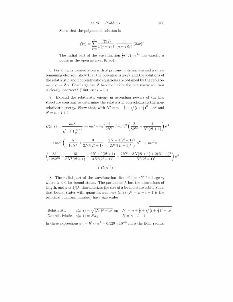
14.13 Problems 285
Show that the polynomial solution is
f(r) =n
∑
j=0
Γ(2γ)
Γ(j + 2γ)
n!
(n− j)!j!(2λr)j
The radial part of the wavefunction 1r r
γf(r)eλr has exactly n
nodes in the open interval (0,∞).
6. For a highly ionized atom with Z protons in its nucleus and a single
remaining electron, show that the potential is Ze/r and the solutions of
the relativistic and nonrelativistic equations are obtained by the replace-
ment α→ Zα. How large can Z become before the relativistic solution
is clearly incorrect? (Hint: set l = 0.)
7. Expand the relativistic energy in ascending powers of the fine
structure constant to determine the relativistic corrections to the non-
relativistic energy. Show that, with N ′ = n+ 12 +
√
(
l + 12
)2 − α2 and
N = n+ l + 1
E(n, l) =mc2
√
1 +(
αN ′
)2→ mc2−mc2 1
2N2α2+mc2
(
3
8N4− 1
N3(2l + 1)
)
α4
+mc2(
− 5
16N6+
3
2N5(2l + 1)− 2N + 3(2l + 1)
2N4(2l + 1)3
)
α6 +mc2×
(
35
128N8− 15
8N7(2l + 1)+
6N + 9(2l+ 1)
4N6(2l+ 1)3− 2N2 + 3N(2l+ 1) + 2(2l+ 1)2
N5(2l + 1)5
)
α8
+ O(α10)
8. The radial part of the wavefunction dies off like eλr for large r,
where λ < 0 for bound states. The parameter λ has the dimensions of
length, and a ≃ 1/|λ| characterizes the size of a bound state orbit. Show
that bound states with quantum numbers (n, l) (N = n + l + 1 is the
principal quantum number) have size scales
Relativistic a(n, l) =√
(N ′)2 + α2 aB N ′ = n+ 12 +
√
(
l + 12
)2 − α2
Nonrelativistic a(n, l) = NaB N = n+ l + 1
In these expressions aB = ~2/me2 = 0.529×10⁻⁸ cm is the Bohr radius:
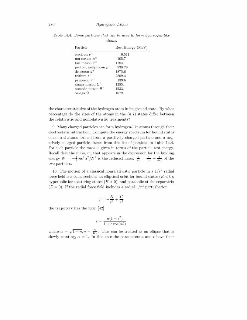
286 Hydrogenic Atoms
Table 14.4. Some particles that can be used to form hydreogen-like
atoms.
Particle Rest Energy (MeV)
electron e± 0.511mu meson µ± 105.7tau meson τ± 1784.proton, antiproton p± 938.26deuteron d+ 1875.6tritium t+ 2809.4pi meson π± 139.6sigma meson Σ± 1385.cascade meson Ξ− 1533.omega Ω− 1672.
the characteristic size of the hydrogen atom in its ground state. By what
percentage do the sizes of the atoms in the (n, l) states differ between
the relativistic and nonrelativistic treatments?
9. Many charged particles can form hydrogen-like atoms through their
electrostatic interaction. Compute the energy spectrum for bound states
of neutral atoms formed from a positively charged particle and a neg-
atively charged particle drawn from this list of particles in Table 14.4.
For each particle the mass is given in terms of the particle rest energy.
Recall that the mass, m, that appears in the expression for the binding
energy W = − 12mc
2α2/N2 is the reduced mass: 1m = 1
m1+ 1
m2of the
two particles.
10. The motion of a classical nonrelativistic particle in a 1/r2 radial
force field is a conic section: an elliptical orbit for bound states (E < 0);
hyperbolic for scattering states (E > 0); and parabolic at the separatrix
(E = 0). If the radial force field includes a radial 1/r3 perturbation
f = −Kr2
+C
r3
the trajectory has the form [42]
r =a(1 − ǫ2)
1 + ǫ cos(αθ)
where α =√
1 − η, η = CKa . This can be treated as an ellipse that is
slowly rotating, α ≃ 1. In this case the parameters a and ǫ have their

14.13 Problems 287
usual meanings for elliptical orbits: a is the semimajor axis and ǫ is the
eccentricity. The ratio η is a measure of the strength of the perturbation
to the strength of the coulomb potential.
a. Expand the relativistic energy E =√
(mc2)2 + (pc)2−K/r to fourth
order in p and show E = (mc2)+(p2/2m)−(p2/2m)2/(2mc2)−K/r = mc2 +W .
b. Replace the quartic term by −(p2/2m)2/(2mc2)by−(W+K/r)2/(2mc2)
and expand. Show that the classical hamiltonian for the motion
of the (special) relativistic particle is
H = mc2 +p2
2m− K ′
r+C′
r2
Evaluate K ′ and C′ and show K ′ = K(1 +W/mc2) and C′ =
−K2/(2mc2).
c. Argue that the classical motion involves a renormalized couplingK →K ′ as well as a 1/r3 component to the force, with C = 2C′.
d. Show that the advance in the perihelion of the orbit is δθ ≃ η/2 per
period.
e. Evaluate η for the planet Mercury, for which ǫ = 0.206 and the
period is T = 0.24 year. Show that this amounts to about 7”
per century. The general relativistic correction is larger by a
factor of 6, and accounts for the observed advance in Mercury’s
perihelion of 42”/century.
f. The existence of precessing elliptical orbits is due to the “relativistic
mass velocity” correction. This can be viewed from two per-
spectives. (1) Newton’s equations are correct and the mass of
the particle varies with its state of motion according to m =
m0/√
1 − (v/c)2. (2) The mass of a particle is a constant of
Nature and Newton’s (nonrelativistic) equations of motion are
not correct for relativistic particles, and must be modified. The
author feels the second interperetation is far superior to the first.
11. When the attracting potential is central and nearly 1/r, the mo-
tion of a bound particle is nearly elliptical. It is useful to describe this
motion as if it were elliptical, with the semimajor axis of the ellipse
precessing in the plane of motion. Assume that the force has the form
F(r) = (−K/r2 + p(r))r, where p(r) is a small perturbation. The rate

288 Hydrogenic Atoms
at which the Runge-Lenz vector precesses is
ω =∂
∂L
(
1
T
∫
p(r) dt
)
=∂
∂L
(
m
LT
∮
r2p(r) dθ
)
with 1/r = mKL2 (1 + M
mK cos θ). Here L is the particle’s orbital angular
momentum and T is its period. If the perturbing term is of the form
C/r3 the integral is C × 2πmKL2 . The perturbations due to Special and
General Relativity are
Special Relativity C =KL2
2m2c2ω =
πK2
TL2c2
General Relativity C = 6 × KL2
2m2c2ω =
6πK2
TL2c2
For planetary motion K = GMm. When M ≫ m, ω is (almost) inde-
pendent of m. Why? Determine how the relativistic precession ω scales
(cf. Problem 16.3, last chapter) with planetary distance from the sun.
What is the precession for the earth? Use ω = 42′′/cent for Mercury
and the following distance ratios:Mercury Venus Earth Mars Jupiter Saturn Uranus Neptune
0.39 0.72 1.00 1.52 5.20 9.54 19.18 30.06
12. The action of the angular momentum shift down operator L−on the lowest m-value spherical harmonic for a given value of l is zero:
L−Ylm=−l(θ, φ) = 0. Use the coordinate representation for L− to com-
pute this function.
a. Write Y lm(θ, φ) = P l
−l(θ)e−ilφ and show
(
− ∂
∂θ+ i
cos θ
sin θ
∂
∂φ
)
P l−l(θ)e
−ilφ = e−ilφ
(
− ∂
∂θ+ l
cos θ
sin θ
∂
∂φ
)
P l−l(θ)
b. Show P l−l = (sin θ)l satisfies this equation.
c. This function is not normalized to unity over the sphere. Normalize
it by introducing a normalization coefficient Nl and enforcing
the condition
∫ π
0
dθ sin θ
∫ 2π
0
dφ|Nl sinl θe−ilφ|2 = 1
d. Show that Nl =√
14π
√
(2l+1)!!(2l)!! .

14.13 Problems 289
e. This leads the the simple recursion relation for normalization coeffi-
cients for the Y l±l(θ, φ):
Nl =
√
2l + 1
2lNl−1
Compare these results with Table 14.2 using initial condition
N0 =√
14π . Compute N3.
f. Use the numerical value of the matrix elements 〈 l
m′ |L+|l
m〉 =
√
(l +m′)(l −m) δm′,m+1 and the coordinate representation of
the shift up operator L+ to construct the correctly normalized
spherical harmonics Y lm(θ, φ).
13. Use methods similar to those described in Problem 12 to construct
the radial wavefunctions for hydrogenic atoms with extreme orbital an-
gular momentum quantum numbers: l = N − 1, where in general the
principle quantum number N = n+ l+1. These functions have no nodes
in the interval (0,∞) (since n = 0).
14. Showd
dt
(r
r
)
=r(r · r) − r(r · r)
r3= −r× (r × r)
r3.
15. r is the position vector from the sun to a planet, or from the
proton to the electron in the hydrogen atom, L = r × p is the orbital
angular momentum, and M is the Laplace-Runge-Lenz vector.
a. M · L = 0.
b. M ·M = 2L·Lm
(
p·p2m − K
r
)
+K2.
c. M · r = L·Lm −Kr.
d. M · r = Mr cos θ.
e. r = L·L/mK1+(M/K) cos θ .
f. Compare this result to the standard solution of the trajectory equa-
tions for motion in a 1/r potential to conclude: L2/mK is the
semimajor axis of the elliptical orbit and ǫ = M/K is the ec-
centricity of the orbit.
g. Conclude that the Laplace-Runge-Lenz vector is a constant of motion
that points to the perihelion of the elliptical orbit.
16. Show that A ·A = −14~2 (L · L + M′ · M′ + L · M′ + M′ · L). Show
that B · B has a similar expression. Show that the two expressions are
equal since L ·M = M · L = 0.

290 Hydrogenic Atoms
17. Show that the inverse of the stereographic projection given in
eq.(14.35) is
p
p0=
u
1 − u ·w
18. Compute px = p ·M/M and py = p ·W/W . Show p2x + (py −
a)2 = r2. Explicitly compute the displacement vector a (i.e., (0, a)) and
the radius r of circular motion. Show that circles in R3 lift to circles
in S3 ⊂ R4 under the stereographic projection of Eq.(14.35). Show
that circles in S3 project back down to circles in R3 under the inverse
transformation.
19. Show that the number of independent monomials of the form
xaybzc, with a, b, c nonnegative integers and a + b + c = l is N(l, 3) =
(l + 3 − 1)/l!(3 − 1)!. In N -dimensional space show that the number
of homogeneous polynomials of degree l in x1, x2, . . . xN is obtained by
replacing 3 → N in this expression. This is the Bose-Einstein counting
statistic.
a. Show that the functions rlY lm(θ, φ) are homogeneous polynomials in
x, y, z of degree l.
b. Show that the number of independent spherical harmonics of degree
l is the difference between the number of homogeneous poly-
nomials of degree l and l − 2 on three variables: dim
Y lm
=
N(l, 3) −N(l − 2, 3) = 2l+ 1.
c. After stereographic transformation into four dimensions, the hydro-
gen wavefunctions in the momentum representation are spher-
ical harmonics in four variables [3]. Show that the number of
spherical harmonics of degree n is dim Ynlm = N(n, 4) −
N(n− 2, 4) = (n+ 1)2.
d. Construct homogeneous polynomials of degree 0, 1, 2 and the spher-
ical harmonics associated with these homogeneous polynomi-
als. Take the inverse Fourier transform of these spherical har-
monics to obtain the hydrogen atom wavefucntions ψ(x)nlm for
n = 0, 1, 2; l = 0, . . . , n− 1; and −l ≤ m ≤ +l.
e. Show that the recursive relation used to build up a Pascal triangle
can be written in the symmetric form
(a+ b+ 1)!
(a+ 12 )!(b + 1
2 )!=
(a+ b)!
(a− 12 )!(b + 1
2 )!+
(a+ b)!
(a+ 12 )!(b− 1
2 )!
where a and b are half odd integers: 12 ,
32 ,
52 , . . . .

14.13 Problems 291
f. Show homogeneous polynomials satisfy the recursion relation:N(l, d) =
N(l, d− 1) +N(l − 1, d).
g. Use this result to derive the following recursion relation for the di-
mensions of the spaces of spherical harmonics on spheres Sn and
Sn−1:
dim Y l(Sn) = dim Y l−1(Sn) + dim Y l(Sn−1)
For the case n = 3 this gives (l + 1)2 = l2 + (2l + 1). The
initialization for all n is Y0(Sn) = 1 = dim Y0(Sn).
h. dim Y l(Sn) = (l+n−2)!l!(n−1)! (2l + n− 1).
20. D-Dimensional Coulomb Problem: In D-dimensional space
the Schrodinger equation for the Kepler problem is Eq. (14.4) in the
relativistic case and Eq. (14.5) in the nonrelativistic case. The only
difference is that the Laplacian ∇2 is on D coordinates rather than
three. In this case the Laplacian operator is
∇2 =
(
1
rD−1/2
∂
∂rrD−1/2
)2
+L2
r2
The angular part of the Laplacian operator, L2, acts on spherical har-
monics on SD−1, Y l(SD−1). These spherical harmonics are eigenfunc-
tions of this (Laplace-Beltrami) operator with eigenvalue −[
(l + α)2 − α2]
,
and α is a quantity that depends on the Lie algebra of SO(D): it is half
the sum over all positive roots of the algebra. For the Lie algebras of the
orthogonal roots the coefficient of the sum that is important is α = D−2.
a. Show that ψ(x) = 1r(D−1)/2Y l(angles) is a clever ansatz that reduces
the Schrodinger equation in D dimensions to the form of Eq.
(14.4) in the relativistic case and Eq. (14.5) in the nonrelativis-
tic case.
b. Show that the only change in Eq.(14.10) is the replacement (l+ 12 )2−
(12 )2 → (l + D−2
2 )2 − (D−22 )2 in column A.
c. Show that the relativistic and nonrelativistic energies shown in Eq.(14.12)
change as follows:
Relativistic N ′ → n+ 12 +
√
(l + 12 )2 + l(D − 3) − α2
Non Relativistic N → n+ 12 +
√
(l + 12 )2 + l(D − 3)
21. Compute the quantum defect in heavy atoms by using the Klein-
Gordon equation and a −1/r2 perturbation. Show that the bound state

292 Hydrogenic Atoms
energy and scattering phase shifts are given by the substitution l(l+1) →l(l+1)−µl. Argue that electrons in the s state penetrate the core much
more deeply (on average) and p-state electrons (than d-state electrons,
...) so that µ0 ≫ µ1 > · · · .
22. The isotropic harmonic oscillator in n dimensions has hamiltonian
H =
n∑
i=1
~ω
(
a†iai +1
2
)
a. Show that the Lie algebra of its geometric symmetry group is spanned
by the angular momentum operators Lij = a†iaj − a†jai = −Lji.
b. Show that the Lie algebra of its dynamical symmetry group is spanned
by the angular momentum operators together with the quadrupole
tensor operators Qij = a†iaj + a†jai = +Qji.
c. Show that one spectrum generating algebra includes the operators
L and Q as well as the single boson operators a†i and aj , as
well as their commutator [ai, a†j] = 1. Show that this algebra is
nonsemisimple and describe its structure.
d. Show that another spectrum generating algebra consists of the op-
erators L and Q as well as the two boson creation operators
a†ia†j and two boson annihilation operators aiaj . Show that this
algebra is simple and describe its structure. Show that this
spectrum generating algebra does not couple all the states that
exist: “parity” is an invariant, where “parity” is even or odd
according to whether the number of excitations in the spectrum
is even or odd.


![Physics 122 – Class #29 (4/30/15)kestrel.nmt.edu/~rsonnenf/phys122/Lectures/S2015Class29.pdfPossible Review Sessions (Clickers) Sat 5/2 9 AM, Workman 113 [A] Sat 5/2 1:30 P M, Workman](https://img.pdfslide.us/doc/110x75/5edabf42434f4178104f901b/physics-122-a-class-29-43015-rsonnenfphys122lecturess2015class29pdf-possible.jpg)