14. CONTINUOUS SENSORS - Karadimov

continuous sensors - 14.1

14. CONTINUOUS SENSORS

14.1 INTRODUCTION

Continuous sensors convert physical phenomena to measurable signals, typically voltages or currents. Consider a simple temperature measuring device, there will be an increase in output voltage proportional to a temperature rise. A computer could measure the voltage, and convert it to a temperature. The basic physical phenomena typically mea-sured with sensors include;

- angular or linear position- acceleration- temperature- pressure or flow rates- stress, strain or force- light intensity- sound

Most of these sensors are based on subtle electrical properties of materials and devices. As a result the signals often require signal conditioners. These are often amplifi-ers that boost currents and voltages to larger voltages.

Sensors are also called transducers. This is because they convert an input phenom-ena to an output in a different form. This transformation relies upon a manufactured device with limitations and imperfection. As a result sensor limitations are often charac-

Topics:

Objectives:• To understand the common continuous sensor types.• To understand interfacing issues.

• Continuous sensor issues; accuracy, resolution, etc.• Angular measurement; potentiometers, encoders and tachometers• Linear measurement; potentiometers, LVDTs, Moire fringes and accelerometers• Force measurement; strain gages and piezoelectric• Liquid and fluid measurement; pressure and flow• Temperature measurement; RTDs, thermocouples and thermistors• Other sensors• Continuous signal inputs and wiring• Glossary


terized with;

Accuracy - This is the maximum difference between the indicated and actual read-ing. For example, if a sensor reads a force of 100N with a ±1% accuracy, then the force could be anywhere from 99N to 101N.

Resolution - Used for systems that step through readings. This is the smallest increment that the sensor can detect, this may also be incorporated into the accuracy value. For example if a sensor measures up to 10 inches of linear dis-placements, and it outputs a number between 0 and 100, then the resolution of the device is 0.1 inches.

Repeatability - When a single sensor condition is made and repeated, there will be a small variation for that particular reading. If we take a statistical range for repeated readings (e.g., ±3 standard deviations) this will be the repeatability. For example, if a flow rate sensor has a repeatability of 0.5cfm, readings for an actual flow of 100cfm should rarely be outside 99.5cfm to 100.5cfm.

Linearity - In a linear sensor the input phenomenon has a linear relationship with the output signal. In most sensors this is a desirable feature. When the relation-ship is not linear, the conversion from the sensor output (e.g., voltage) to a cal-culated quantity (e.g., force) becomes more complex.

Precision - This considers accuracy, resolution and repeatability or one device rel-ative to another.

Range - Natural limits for the sensor. For example, a sensor for reading angular rotation may only rotate 200 degrees.

Dynamic Response - The frequency range for regular operation of the sensor. Typ-ically sensors will have an upper operation frequency, occasionally there will be lower frequency limits. For example, our ears hear best between 10Hz and 16KHz.

Environmental - Sensors all have some limitations over factors such as tempera-ture, humidity, dirt/oil, corrosives and pressures. For example many sensors will work in relative humidities (RH) from 10% to 80%.

Calibration - When manufactured or installed, many sensors will need some cali-bration to determine or set the relationship between the input phenomena, and output. For example, a temperature reading sensor may need to be zeroed or adjusted so that the measured temperature matches the actual temperature. This may require special equipment, and need to be performed frequently.

Cost - Generally more precision costs more. Some sensors are very inexpensive, but the signal conditioning equipment costs are significant.

14.2 INDUSTRIAL SENSORS

This section describes sensors that will be of use for industrial measurements. The sections have been divided by the phenomena to be measured. Where possible details are provided.


14.2.1 Angular Displacement

14.2.1.1 - Potentiometers

Potentiometers measure the angular position of a shaft using a variable resistor. A potentiometer is shown in Figure 14.1. The potentiometer is resistor, normally made with a thin film of resistive material. A wiper can be moved along the surface of the resistive film. As the wiper moves toward one end there will be a change in resistance proportional to the distance moved. If a voltage is applied across the resistor, the voltage at the wiper interpolate the voltages at the ends of the resistor.

Figure 14.1 A Potentiometer

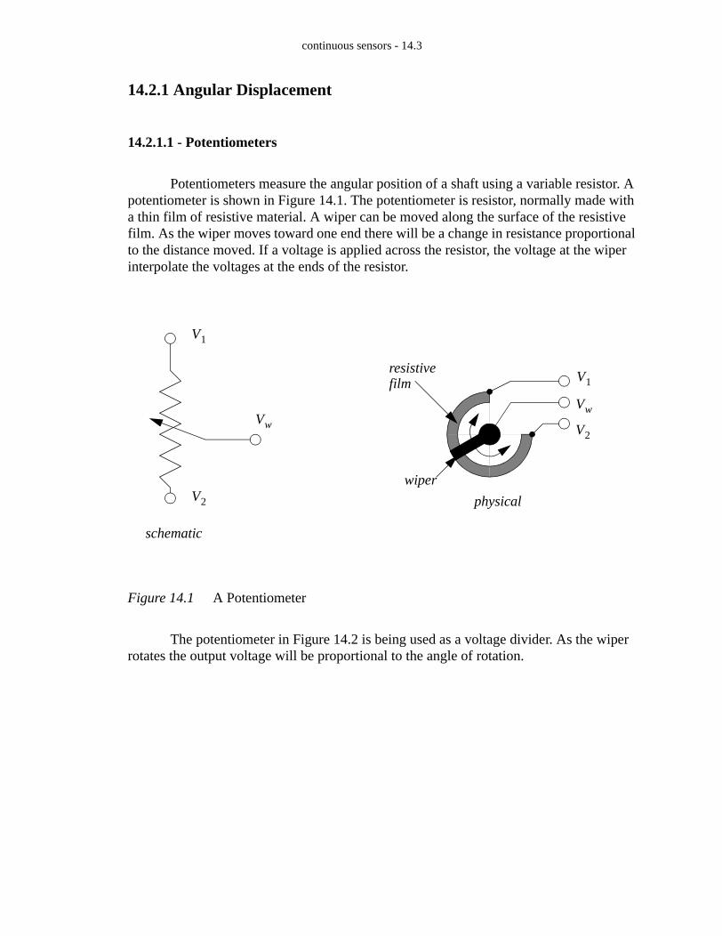
The potentiometer in Figure 14.2 is being used as a voltage divider. As the wiper rotates the output voltage will be proportional to the angle of rotation.

schematic

physical

resistive

wiper

film

V1

V2

Vw

V1

Vw

V2


Figure 14.2 A Potentiometer as a Voltage Divider

Potentiometers are popular because they are inexpensive, and don’t require special signal conditioners. But, they have limited accuracy, normally in the range of 1% and they are subject to mechanical wear.

Potentiometers measure absolute position, and they are calibrated by rotating them in their mounting brackets, and then tightening them in place. The range of rotation is nor-mally limited to less than 360 degrees or multiples of 360 degrees. Some potentiometers can rotate without limits, and the wiper will jump from one end of the resistor to the other.

Faults in potentiometers can be detected by designing the potentiometer to never reach the ends of the range of motion. If an output voltage from the potentiometer ever reaches either end of the range, then a problem has occurred, and the machine can be shut down. Two examples of problems that might cause this are wires that fall off, or the poten-tiometer rotates in its mounting.

14.2.2 Encoders

Encoders use rotating disks with optical windows, as shown in Figure 14.3. The encoder contains an optical disk with fine windows etched into it. Light from emitters passes through the openings in the disk to detectors. As the encoder shaft is rotated, the light beams are broken. The encoder shown here is a quadrature encode, and it will be dis-cussed later.

V2

V1

Vout

Vout V2 V1–( )θw

θmax----------- V1+=

θmax θw


Figure 14.3 An Encoder Disk

There are two fundamental types of encoders; absolute and incremental. An abso-lute encoder will measure the position of the shaft for a single rotation. The same shaft angle will always produce the same reading. The output is normally a binary or grey code number. An incremental (or relative) encoder will output two pulses that can be used to determine displacement. Logic circuits or software is used to determine the direction of rotation, and count pulses to determine the displacement. The velocity can be determined by measuring the time between pulses.

Encoder disks are shown in Figure 14.4. The absolute encoder has two rings, the outer ring is the most significant digit of the encoder, the inner ring is the least significant digit. The relative encoder has two rings, with one ring rotated a few degrees ahead of the other, but otherwise the same. Both rings detect position to a quarter of the disk. To add accuracy to the absolute encoder more rings must be added to the disk, and more emitters and detectors. To add accuracy to the relative encoder we only need to add more windows to the existing two rings. Typical encoders will have from 2 to thousands of windows per ring.

lightemitters

lightdetectors

Shaft rotates

Note: this type of encoder is commonly used in com-puter mice with a roller ball.


Figure 14.4 Encoder Disks

When using absolute encoders, the position during a single rotation is measured directly. If the encoder rotates multiple times then the total number of rotations must be counted separately.

When using a relative encoder, the distance of rotation is determined by counting the pulses from one of the rings. If the encoder only rotates in one direction then a simple count of pulses from one ring will determine the total distance. If the encoder can rotate both directions a second ring must be used to determine when to subtract pulses. The quadrature scheme, using two rings, is shown in Figure 14.5. The signals are set up so that one is out of phase with the other. Notice that for different directions of rotation, input B either leads or lags A.

relative encoder

absolute encoder(quadrature)

sensors read acrossa single radial line


Figure 14.5 Quadrature Encoders

Interfaces for encoders are commonly available for PLCs and as purchased units. Newer PLCs will also allow two normal inputs to be used to decode encoder inputs.

Quad input A

Quad Input B

total displacement can be determined

Quad input A

Quad Input B

Note the changeas directionis reversed

by adding/subtracting pulse counts(direction determines add/subtract)

Note: To determine direction we can do a simple check. If both are off or on, the first to change state determines direction. Consider a point in the graphs above where both A and B are off. If A is the first input to turn on the encoder is rotating clockwise. If B is the first to turn on the rotation is counterclockwise.

clockwise rotation

counterclockwise rotation

Aside: A circuit (or program) can be built for this circuit using an up/down counter. If the positive edge of input A is used to trigger the clock, and input B is used to drive the up/down count, the counter will keep track of the encoder position.


Normally absolute and relative encoders require a calibration phase when a con-troller is turned on. This normally involves moving an axis until it reaches a logical sensor that marks the end of the range. The end of range is then used as the zero position. Machines using encoders, and other relative sensors, are noticeable in that they normally move to some extreme position before use.

14.2.2.1 - Tachometers

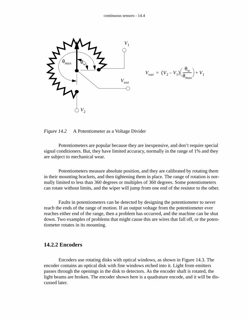
Tachometers measure the velocity of a rotating shaft. A common technique is to mount a magnet to a rotating shaft. When the magnetic moves past a stationary pick-up coil, current is induced. For each rotation of the shaft there is a pulse in the coil, as shown in Figure 14.6. When the time between the pulses is measured the period for one rotation can be found, and the frequency calculated. This technique often requires some signal conditioning circuitry.

Figure 14.6 A Magnetic Tachometer

Another common technique uses a simple permanent magnet DC generator (note: you can also use a small DC motor). The generator is hooked to the rotating shaft. The rotation of a shaft will induce a voltage proportional to the angular velocity. This tech-nique will introduce some drag into the system, and is used where efficiency is not an issue.

Both of these techniques are common, and inexpensive.

14.2.3 Linear Position

14.2.3.1 - Potentiometers

rotatingshaft

magnet

pickupcoil

Vout

Vout

t

1/f


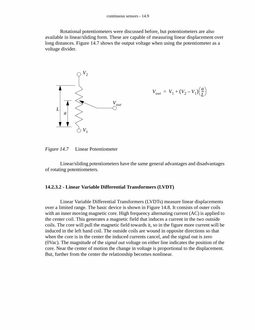
Rotational potentiometers were discussed before, but potentiometers are also available in linear/sliding form. These are capable of measuring linear displacement over long distances. Figure 14.7 shows the output voltage when using the potentiometer as a voltage divider.

Figure 14.7 Linear Potentiometer

Linear/sliding potentiometers have the same general advantages and disadvantages of rotating potentiometers.

14.2.3.2 - Linear Variable Differential Transformers (LVDT)

Linear Variable Differential Transformers (LVDTs) measure linear displacements over a limited range. The basic device is shown in Figure 14.8. It consists of outer coils with an inner moving magnetic core. High frequency alternating current (AC) is applied to the center coil. This generates a magnetic field that induces a current in the two outside coils. The core will pull the magnetic field towards it, so in the figure more current will be induced in the left hand coil. The outside coils are wound in opposite directions so that when the core is in the center the induced currents cancel, and the signal out is zero (0Vac). The magnitude of the signal out voltage on either line indicates the position of the core. Near the center of motion the change in voltage is proportional to the displacement. But, further from the center the relationship becomes nonlinear.

La

V1

V2

Vout

Vout V1 V2 V1–( ) aL--- +=


Figure 14.8 An LVDT

Figure 14.9 A Simple Signal Conditioner for an LVDT

These devices are more accurate than linear potentiometers, and have less friction. Typical applications for these devices include measuring dimensions on parts for quality

AC input

signal out

A rod drivesthe sliding core

∆x

∆V K∆x=

where,

∆V output voltage=

K constant for device=

∆x core displacement=

LVDTVac in

Vac out Vdc out

Aside: The circuit below can be used to produce a voltage that is proportional to position. The two diodes convert the AC wave to a half wave DC wave. The capacitor and resis-tor values can be selected to act as a low pass filter. The final capacitor should be large enough to smooth out the voltage ripple on the output.


control. They are often used for pressure measurements with Bourdon tubes and bellows/diaphragms. A major disadvantage of these sensors is the high cost, often in the thousands.

14.2.3.3 - Moire Fringes

High precision linear displacement measurements can be made with Moire Fringes, as shown in Figure 14.10. Both of the strips are transparent (or reflective), with black lines at measured intervals. The spacing of the lines determines the accuracy of the position measurements. The stationary strip is offset at an angle so that the strips interfere to give irregular patterns. As the moving strip travels by a stationary strip the patterns will move up, or down, depending upon the speed and direction of motion.

Figure 14.10 The Moire Fringe Effect

A device to measure the motion of the moire fringes is shown in Figure 14.11. A light source is collimated by passing it through a narrow slit to make it one slit width. This is then passed through the fringes to be detected by light sensors. At least two light sensors are needed to detect the bright and dark locations. Two sensors, close enough, can act as a quadrature pair, and the same method used for quadrature encoders can be used to deter-mine direction and distance of motion.

Note: you can recreate this effect with the strips below. Photocopy the pattern twice, overlay the sheets and hold them up to the light. You will notice that shifting one sheet will cause the stripes to move up or down.

MovingStationary


Figure 14.11 Measuring Motion with Moire Fringes

These are used in high precision applications over long distances, often meters. They can be purchased from a number of suppliers, but the cost will be high. Typical applications include Coordinate Measuring Machines (CMMs).

14.2.3.4 - Accelerometers

Accelerometers measure acceleration using a mass suspended on a force sensor, as shown in Figure 14.12. When the sensor accelerates, the inertial resistance of the mass will cause the force sensor to deflect. By measuring the deflection the acceleration can be determined. In this case the mass is cantilevered on the force sensor. A base and housing enclose the sensor. A small mounting stud (a threaded shaft) is used to mount the acceler-ometer.

Figure 14.12 A Cross Section of an Accelerometer

Accelerometers are dynamic sensors, typically used for measuring vibrations

onoffonoff

MassForceSensor

Base

MountingStud Housing


between 10Hz to 10KHz. Temperature variations will affect the accuracy of the sensors. Standard accelerometers can be linear up to 100,000 m/s**2: high shock designs can be used up to 1,000,000 m/s**2. There is often a trade-off between a wide frequency range and device sensitivity (note: higher sensitivity requires a larger mass). Figure 14.13 shows the sensitivity of two accelerometers with different resonant frequencies. A smaller reso-nant frequency limits the maximum frequency for the reading. The smaller frequency results in a smaller sensitivity. The units for sensitivity is charge per m/s**2.

Figure 14.13 Piezoelectric Accelerometer Sensitivities

The force sensor is often a small piece of piezoelectric material (discussed later in this chapter). The piezoelectic material can be used to measure the force in shear or com-pression. Piezoelectric based accelerometers typically have parameters such as,

-100 to 250°C operating range1mV/g to 30V/g sensitivityoperate well below one forth of the natural frequency

The accelerometer is mounted on the vibration source as shown in Figure 14.14. The accelerometer is electrically isolated from the vibration source so that the sensor may be grounded at the amplifier (to reduce electrical noise). Cables are fixed to the surface of the vibration source, close to the accelerometer, and are fixed to the surface as often as possible to prevent noise from the cable striking the surface. Background vibrations can be detected by attaching control electrodes to non-vibrating surfaces. Each accelerometer is different, but some general application guidelines are;

• The control vibrations should be less than 1/3 of the signal for the error to be less than 12%).

• Mass of the accelerometers should be less than a tenth of the measurement mass.• These devices can be calibrated with shakers, for example a 1g shaker will hit a

peak velocity of 9.81 m/s**2.

sensitivity

4.5 pC/(m/s**2).004

resonant freq. (Hz)

22 KHz180KHz


Figure 14.14 Mounting an Accelerometer

Equipment normally used when doing vibration testing is shown in Figure 14.15. The sensor needs to be mounted on the equipment to be tested. A pre-amplifier normally converts the charge generated by the accelerometer to a voltage. The voltage can then be analyzed to determine the vibration frequencies.

Figure 14.15 Typical Connection for Accelerometers

Accelerometers are commonly used for control systems that adjust speeds to reduce vibration and noise. Computer Controlled Milling machines now use these sensors to actively eliminate chatter, and detect tool failure. The signal from accelerometers can be

accelerometerisolated

isolated

surface

hookup wire

waferstud

Sealant to prevent moisture

pre-amp

signal processor/recorder

Source of vibrations,or site for vibrationmeasurement

Sensor

control system


integrated to find velocity and acceleration.

Currently accelerometers cost hundreds or thousands per channel. But, advances in micromachining are already beginning to provide integrated circuit accelerometers at a low cost. Their current use is for airbag deployment systems in automobiles.

14.2.4 Forces and Moments

14.2.4.1 - Strain Gages

Strain gages measure strain in materials using the change in resistance of a wire. The wire is glued to the surface of a part, so that it undergoes the same strain as the part (at the mount point). Figure 14.16 shows the basic properties of the undeformed wire. Basi-cally, the resistance of the wire is a function of the resistivity, length, and cross sectional area.

Figure 14.16 The Electrical Properties of a Wire

+

-

V

I

t

w

L

RVI--- ρL

A--- ρ L

wt------= = =

where,

R resistance of wire=

V I, voltage and current=

L length of wire=

w t, width and thickness=

A cross sectional area of conductor=

ρ resistivity of material=


After the wire in Figure 14.16 has been deformed it will take on the new dimen-sions and resistance shown in Figure 14.17. If a force is applied as shown, the wire will become longer, as predicted by Young’s modulus. But, the cross sectional area will decrease, as predicted by Poison’s ratio. The new length and cross sectional area can then be used to find a new resistance.

Figure 14.17 The Electrical and Mechanical Properties of the Deformed Wire

t’

w’

L’

R' ρ L'w't'-------- ρ L 1 ε+( )

w 1 νε–( )t 1 νε–( )---------------------------------------------- = =

where,

ν poissons ratio for the material=

F applied force=

E Youngs modulus for the material=

σ ε, stress and strain of material=

F

σ FA--- F

wt------ Eε= = =

∆R∴ R' R– R1 ε+( )

1 νε–( ) 1 νε–( )---------------------------------------- 1–= =

ε∴ FEwt----------=

Aside: Gauge factor, as defined below, is a commonly used measure of stain gauge sensitivity.

GF

∆RR

-------

ε-------------=


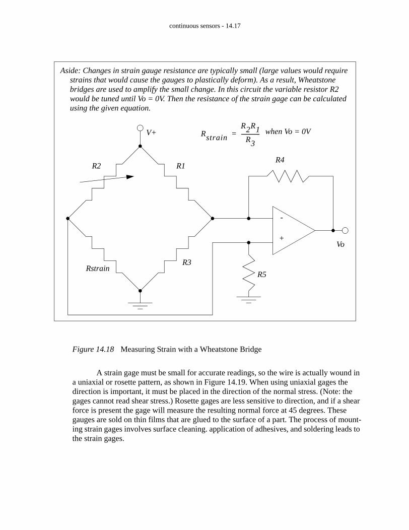
Figure 14.18 Measuring Strain with a Wheatstone Bridge

A strain gage must be small for accurate readings, so the wire is actually wound in a uniaxial or rosette pattern, as shown in Figure 14.19. When using uniaxial gages the direction is important, it must be placed in the direction of the normal stress. (Note: the gages cannot read shear stress.) Rosette gages are less sensitive to direction, and if a shear force is present the gage will measure the resulting normal force at 45 degrees. These gauges are sold on thin films that are glued to the surface of a part. The process of mount-ing strain gages involves surface cleaning. application of adhesives, and soldering leads to the strain gages.

R4

R5

R1

R3

R2

Rstrain

Vo

V+

-

+

Aside: Changes in strain gauge resistance are typically small (large values would require strains that would cause the gauges to plastically deform). As a result, Wheatstone bridges are used to amplify the small change. In this circuit the variable resistor R2 would be tuned until Vo = 0V. Then the resistance of the strain gage can be calculated using the given equation.

Rstrain

R2R1R3

--------------= when Vo = 0V


Figure 14.19 Wire Arrangements in Strain Gages

A design techniques using strain gages is to design a part with a narrowed neck to mount the strain gage on, as shown in Figure 14.20. In the narrow neck the strain is pro-portional to the load on the member, so it may be used to measure force. These parts are often called load cells.

Figure 14.20 Using a Narrow to Increase Strain

Strain gauges are inexpensive, and can be used to measure a wide range of stresses with accuracies under 1%. Gages require calibration before each use. This often involves making a reading with no load, or a known load applied. An example application includes using strain gages to measure die forces during stamping to estimate when maintenance is needed.

14.2.4.2 - Piezoelectric

When a crystal undergoes strain it displaces a small amount of charge. In other words, when the distance between atoms in the crystal lattice changes some electrons are forced out or drawn in. This also changes the capacitance of the crystal. This is known as

uniaxial rosette

stre

ssdi

rect

ion

F F

mounted in narrow sectionto increase strain effect


the Piezoelectric effect. Figure 14.21 shows the relationships for a crystal undergoing a linear deformation. The charge generated is a function of the force applied, the strain in the material, and a constant specific to the material. The change in capacitance is propor-tional to the change in the thickness.

Figure 14.21 The Piezoelectric Effect

These crystals are used for force sensors, but they are also used for applications such as microphones and pressure sensors. Applying an electrical charge can induce strain, allowing them to be used as actuators, such as audio speakers.

When using piezoelectric sensors charge amplifiers are needed to convert the small amount of charge to a larger voltage. These sensors are best suited to dynamic measure-ments, when used for static measurements they tend to drift or slowly lose charge, and the signal value will change.

b

c a

F

F

+q-

where,

Cεab

c---------=

C capacitance change=

a b c, , geometry of material=

ε dielectric constant (quartz typ. 4.06*10**-11 F/m)=

i current generated=

F force applied=

g constant for material (quartz typ. 50*10**-3 Vm/N)=

E Youngs modulus (quartz typ. 8.6*10**10 N/m**2)=

i εgddt-----F=


14.2.5 Liquids and Gases

There are a number of factors to be considered when examining liquids and gasses.

• Flow velocity• Density• Viscosity• Pressure

There are a number of differences factors to be considered when dealing with flu-ids and gases. Normally a fluid is considered incompressible, while a gas normally fol-lows the ideal gas law. Also, given sufficiently high enough temperatures, or low enough pressures a fluid can be come a liquid.

When flowing, the flow may be smooth, or laminar. In case of high flow rates or unrestricted flow, turbulence may result. The Reynold’s number is used to determine the transition to turbulence. The equation below is for calculation the Reynold’s number for fluid flow in a pipe. A value below 2000 will result in laminar flow. At a value of about 3000 the fluid flow will become uneven. At a value between 7000 and 8000 the flow will become turbulent.

PV nRT=

where,P the gas pressure=

V the volume of the gas=

n the number of moles of the gas=

R the ideal gas constant= =

T the gas temperature=


14.2.5.1 - Pressure

Figure 14.22 shows different two mechanisms for pressure measurement. The Bourdon tube uses a circular pressure tube. When the pressure inside is higher than the surrounding air pressure (14.7psi approx.) the tube will straighten. A position sensor, con-nected to the end of the tube, will be elongated when the pressure increases.

Figure 14.22 Pressure Transducers

RVDρ

u------------=

where,

R Reynolds number=

V velocity=

D pipe diameter=

ρ fluid density=

u viscosity=

pressure

a) Bourdon Tube

posi

tion

sens

or

position sensor

pressure

b) Baffle

pressureincrease

pressureincrease


These sensors are very common and have typical accuracies of 0.5%.

14.2.5.2 - Venturi Valves

When a flowing fluid or gas passes through a narrow pipe section (neck) the pres-sure drops. If there is no flow the pressure before and after the neck will be the same. The faster the fluid flow, the greater the pressure difference before and after the neck. This is known as a Venturi valve. Figure 14.23 shows a Venturi valve being used to measure a fluid flow rate. The fluid flow rate will be proportional to the pressure difference before and at the neck (or after the neck) of the valve.

Figure 14.23 A Venturi Valve

differential

fluid flow

pressuretransducer


Figure 14.24 The Pressure Relationship for a Venturi Valve

Venturi valves allow pressures to be read without moving parts, which makes them very reliable and durable. They work well for both fluids and gases. It is also common to use Venturi valves to generate vacuums for actuators, such as suction cups.

14.2.5.3 - Coriolis Flow Meter

Fluid passes through thin tubes, causing them to vibrate. As the fluid approaches the point of maximum vibration it accelerates. When leaving the point it decelerates. The

Aside: Bernoulli’s equation can be used to relate the pressure drop in a venturi valve.

where,

pρ--- v

2

2----- gz+ + C=

p pressure=

ρ density=

v velocity=

g gravitational constant=

z height above a reference=

C constant=

pbefore

ρ----------------

vbefore2

2------------------ gz+ + C

pafter

ρ------------

vafter2

2-------------- gz+ += =

Consider the centerline of the fluid flow through the valve. Assume the fluid is incompress-ible, so the density does not change. And, assume that the center line of the valve does not change. This gives us a simpler equation, as shown below, that relates the velocity and pressure before and after it is compressed.

pbefore

ρ----------------

vbefore2

2------------------+

pafter

ρ------------

vafter2

2--------------+=

pbefore pafter– ρvafter

2

2--------------

vbefore2

2------------------–

=

The flow velocity v in the valve will be larger than the velocity in the larger pipe sec-tion before. So, the right hand side of the expression will be positive. This will mean that the pressure before will always be higher than the pressure after, and the differ-ence will be proportional to the velocity squared.


result is a distributed force that causes a bending moment, and hence twisting of the pipe. The amount of bending is proportional to the velocity of the fluid flow. These devices typ-ically have a large constriction on the flow, and result is significant loses. Some of the devices also use bent tubes to increase the sensitivity, but this also increases the flow resis-tance. The typical accuracy for a Coriolis flowmeter is 0.1%.

14.2.5.4 - Magnetic Flow Meter

A magnetic sensor applies a magnetic field perpendicular to the flow of a conduc-tive fluid. As the fluid moves, the electrons in the fluid experience an electromotive force. The result is that a potential (voltage) can be measured perpendicular to the direction of the flow and the magnetic field. The higher the flow rate, the greater the voltage. The typ-ical accuracy for these sensors is 0.5%.

These flowmeters don’t oppose fluid flow, and so they don’t result in pressure drops.

14.2.5.5 - Ultrasonic Flow Meter

A transmitter emits a high frequency sound at point on a tube. The signal must then pass through the fluid to a detector where it is picked up. If the fluid is flowing in the same direction as the sound it will arrive sooner. If the sound is against the flow it will take longer to arrive. In a transit time flow meter two sounds are used, one traveling forward, and the other in the opposite direction. The difference in travel time for the sounds is used to determine the flow velocity.

A doppler flowmeter bounces a soundwave off particle in a flow. If the particle is moving away from the emitter and detector pair, then the detected frequency will be low-ered, if it is moving towards them the frequency will be higher.

The transmitter and receiver have a minimal impact on the fluid flow, and there-fore don’t result in pressure drops.

14.2.5.6 - Vortex Flow Meter

Fluid flowing past a large (typically flat) obstacle will shed vortices. The fre-quency of the vortices will be proportional to the flow rate. Measuring the frequency allows an estimate of the flow rate. These sensors tend be low cost and are popular for low accuracy applications.


14.2.5.7 - Positive Displacement Meters

In some cases more precise readings of flow rates and volumes may be required. These can be obtained by using a positive displacement meter. In effect these meters are like pumps run in reverse. As the fluid is pushed through the meter it produces a measur-able output, normally on a rotating shaft.

14.2.5.8 - Pitot Tubes

Gas flow rates can be measured using Pitot tubes, as shown in Figure 14.25. These are small tubes that project into a flow. The diameter of the tube is small (typically less than 1/8") so that it doesn’t affect the flow.

Figure 14.25 Pitot Tubes for Measuring Gas Flow Rates

14.2.6 Temperature

Temperature measurements are very common with control systems. The tempera-ture ranges are normally described with the following classifications.

very low temperatures <-60 deg C - e.g. superconductors in MRI unitslow temperature measurement -60 to 0 deg C - e.g. freezer controlsfine temperature measurements 0 to 100 deg C - e.g. environmental controlshigh temperature measurements <3000 deg F - e.g. metal refining/processing

gas flow

pitot

connecting hose pressuresensor

tube


very high temperatures > 2000 deg C - e.g. plasma systems

14.2.6.1 - Resistive Temperature Detectors (RTDs)

When a metal wire is heated the resistance increases. So, a temperature can be measured using the resistance of a wire. Resistive Temperature Detectors (RTDs) nor-mally use a wire or film of platinum, nickel, copper or nickel-iron alloys. The metals are wound or wrapped over an insulator, and covered for protection. The resistances of these alloys are shown in Figure 14.26.

Figure 14.26 RTD Properties

These devices have positive temperature coefficients that cause resistance to increase linearly with temperature. A platinum RTD might have a resistance of 100 ohms at 0C, that will increase by 0.4 ohms/°C. The total resistance of an RTD might double over the temperature range.

A current must be passed through the RTD to measure the resistance. (Note: a volt-age divider can be used to convert the resistance to a voltage.) The current through the RTD should be kept to a minimum to prevent self heating. These devices are more linear than thermocouples, and can have accuracies of 0.05%. But, they can be expensive

14.2.6.2 - Thermocouples

Each metal has a natural potential level, and when two different metals touch there is a small potential difference, a voltage. (Note: when designing assemblies, dissimilar metals should not touch, this will lead to corrosion.) Thermocouples use a junction of dis-similar metals to generate a voltage proportional to temperature. This principle was dis-covered by T.J. Seebeck.

The basic calculations for thermocouples are shown in Figure 14.27. This calcula-tion provides the measured voltage using a reference temperature and a constant specific

Material

PlatinumNickelCopper

Typical

10012010

Temperature

-200 - 850 (-328 - 1562)-80 - 300 (-112 - 572)-200 - 260 (-328 - 500)

Resistance (ohms)

Range C (F)


to the device. The equation can also be rearranged to provide a temperature given a volt-age.

Figure 14.27 Thermocouple Calculations

The list in Table 1 shows different junction types, and the normal temperature ranges. Both thermocouples, and signal conditioners are commonly available, and rela-tively inexpensive. For example, most PLC vendors sell thermocouple input cards that will allow multiple inputs into the PLC.

Table 1: Thermocouple Types

ANSIType

MaterialsTemperature

Range(°F)

Voltage Range(mV)

T copper/constantan -200 to 400 -5.60 to 17.82

J iron/constantan 0 to 870 0 to 42.28

E chromel/constantan -200 to 900 -8.82 to 68.78

K chromel/aluminum -200 to 1250 -5.97 to 50.63

R platinum-13%rhodium/platinum 0 to 1450 0 to 16.74

S platinum-10%rhodium/platinum 0 to 1450 0 to 14.97

C tungsten-5%rhenium/tungsten-26%rhenium 0 to 2760 0 to 37.07

Vout α T Tref–( )=

where,α constant (V/C)=

T Tref, current and reference temperatures=

50µV°C------- (typical)

measuringdevice

+- Vout

T∴Vout

α---------- Tref+=


Figure 14.28 Thermocouple Temperature Voltage Relationships (Approximate)

The junction where the thermocouple is connected to the measurement instrument is normally cooled to reduce the thermocouple effects at those junctions. When using a thermocouple for precision measurement, a second thermocouple can be kept at a known temperature for reference. A series of thermocouples connected together in series pro-duces a higher voltage and is called a thermopile. Readings can approach an accuracy of 0.5%.

14.2.6.3 - Thermistors

Thermistors are non-linear devices, their resistance will decrease with an increase in temperature. (Note: this is because the extra heat reduces electron mobility in the semi-conductor.) The resistance can change by more than 1000 times. The basic calculation is shown in Figure 14.29.

often metal oxide semiconductors The calculation uses a reference temperature and resistance, with a constant for the device, to predict the resistance at another tempera-ture. The expression can be rearranged to calculate the temperature given the resistance.

20

40

60

80

0

0 500 1000 1500 2000 2500

E

J

K

T

C

RS

°F( )

mV


Figure 14.29 Thermistor Calculations

Figure 14.30 Thermistor Signal Conditioning Circuit

Rt Roeβ 1

T--- 1

To

-----–

=

where,

Ro Rt, resistances at reference and measured temps.=

To T, reference and actual temperatures=

β constant for device=

T∴βTo

To

Rt

Ro------ ln β+

---------------------------------=

+V

Vout+

-

R1

R2

R3

R4

R5

Aside: The circuit below can be used to convert the resistance of the thermistor to a volt-age using a Wheatstone bridge and an inverting amplifier.


Thermistors are small, inexpensive devices that are often made as beads, or metal-lized surfaces. The devices respond quickly to temperature changes, and they have a higher resistance, so junction effects are not an issue. Typical accuracies are 1%, but the devices are not linear, have a limited temperature/resistance range and can be self heating.

14.2.6.4 - Other Sensors

IC sensors are becoming more popular. They output a digital reading and can have accuracies better than 0.01%. But, they have limited temperature ranges, and require some knowledge of interfacing methods for serial or parallel data.

Pyrometers are non-contact temperature measuring devices that use radiated heat. These are normally used for high temperature applications, or for production lines where it is not possible to mount other sensors to the material.

14.2.7 Light

14.2.7.1 - Light Dependant Resistors (LDR)

Light dependant resistors (LDRs) change from high resistance (>Mohms) in bright light to low resistance (<Kohms) in the dark. The change in resistance is non-linear, and is also relatively slow (ms).


Figure 14.31 A Light Level Detector Circuit

14.2.8 Chemical

14.2.8.1 - pH

The pH of an ionic fluid can be measured over the range from a strong base (alka-line) with pH=14, to a neutral value, pH=7, to a strong acid, pH=0. These measurements are normally made with electrodes that are in direct contact with the fluids.

14.2.8.2 - Conductivity

Conductivity of a material, often a liquid is often used to detect impurities. This can be measured directly be applying a voltage across two plates submerged in the liquid and measuring the current. High frequency inductive fields is another alternative.

Vhigh

Vout

Vlow

Aside: an LDR can be used in a voltage divider to convert the change in resistance to a measurable voltage.

These are common in low cost night lights.


14.2.9 Others

A number of other detectors/sensors are listed below,

Combustion - gases such as CO2 can be an indicator of combustion Humidity - normally in gasesDew Point - to determine when condensation will form

14.3 INPUT ISSUES

Signals from sensors are often not in a form that can be directly input to a control-ler. In these cases it may be necessary to buy or build signal conditioners. Normally, a sig-nal conditioner is an amplifier, but it may also include noise filters, and circuitry to convert from current to voltage. This section will discuss the electrical and electronic interfaces between sensors and controllers.

Analog signal are prone to electrical noise problems. This is often caused by elec-tromagnetic fields on the factory floor inducing currents in exposed conductors. Some of the techniques for dealing with electrical noise include;

twisted pairs - the wires are twisted to reduce the noise induced by magnetic fields.shielding - shielding is used to reduce the effects of electromagnetic interference.single/double ended inputs - shared or isolated reference voltages (commons).

When a signal is transmitted through a wire, it must return along another path. If the wires have an area between them the magnetic flux enclosed in the loop can induce current flow and voltages. If the wires are twisted, a few times per inch, then the amount of noise induced is reduced. This technique is common in signal wires and network cables.

A shielded cable has a metal sheath, as shown in Figure 14.32. This sheath needs to be connected to the measuring device to allow induced currents to be passed to ground. This prevents electromagnetic waves to induce voltages in the signal wires.


Figure 14.32 Cable Shielding

When connecting analog voltage sources to a controller the common, or reference voltage can be connected different ways, as shown in Figure 14.33. The least expensive method uses one shared common for all analog signals, this is called single ended. The more accurate method is to use separate commons for each signal, this is called double ended. Most analog input cards allow a choice between one or the other. But, when double ended inputs are used the number of available inputs is halved. Most analog output cards are double ended.

Analog voltage source

+-

IN1

REF1

SHLD

Analog InputA Shield is a metal sheath thatsurrounds the wires


Figure 14.33 Single and Double Ended Inputs

Signals from transducers are typically too small to be read by a normal analog input card. Amplifiers are used to increase the magnitude of these signals. An example of a single ended signal amplifier is shown in Figure 14.34. The amplifier is in an inverting configuration, so the output will have an opposite sign from the input. Adjustments are provided for gain and offset adjustments.

Ain 0

Ain 1

Ain 2

Ain 3

Ain 4

Ain 5

Ain 6

Ain 7

COM

device +-#1

device +-#1

Ain 0

Ain 0

Ain 1

Ain 1

Ain 2

Ain 2

Ain 3

Ain 3

device +-#1

device +-#1

Single ended - with this arrangement the signal quality can be poorer, but more inputs are available.

Double ended - with this arrangement the signal quality can be better, but fewer inputs are available.

Note: op-amps are used in this section to implement the amplifiers because they are inexpensive, common, and well suited to simple design and construction projects. When purchasing a commercial signal conditioner, the circuitry will be more com-plex, and include other circuitry for other factors such as temperature compensation.


Figure 14.34 A Single Ended Signal Amplifier

A differential amplifier with a current input is shown in Figure 14.35. Note that Rc converts a current to a voltage. The voltage is then amplified to a larger voltage.

Figure 14.35 A Current Amplifier

Vin

+V

-V

Ro

Ri

Rf Rg

gain

Vout

-+

offset

Vout

Rf Rg+

Ri----------------- Vin offset+=

-+Iin

Vout

RcR1

R2

Rf

R3

R4


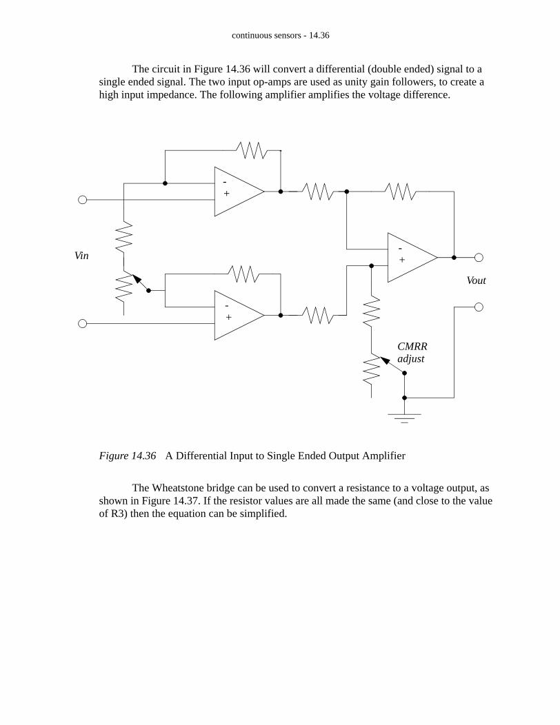
The circuit in Figure 14.36 will convert a differential (double ended) signal to a single ended signal. The two input op-amps are used as unity gain followers, to create a high input impedance. The following amplifier amplifies the voltage difference.

Figure 14.36 A Differential Input to Single Ended Output Amplifier

The Wheatstone bridge can be used to convert a resistance to a voltage output, as shown in Figure 14.37. If the resistor values are all made the same (and close to the value of R3) then the equation can be simplified.

Vin

Vout

-+

-+

-+

CMRRadjust


Figure 14.37 A Resistance to Voltage Amplifier

14.4 SENSOR GLOSSARY

Ammeter - A meter to indicate electrical current. It is normally part of a DMMBellows - This is a flexible volumed that will expand or contract with a pressure

change. This often looks like a cylinder with a large radius (typ. 2") but it is very thin (type 1/4"). It can be set up so that when pressure changes, the dis-placement of one side can be measured to determine pressure.

Bourdon tube - Widely used industrial gage to measure pressure and vacuum. It resembles a crescent moon. When the pressure inside changes the moon shape will tend to straighten out. By measuring the displacement of the tip the pres-sure can be measured.

Chromatographic instruments - laboratory-type instruments used to analyze chem-ical compounds and gases.

Inductance-coil pulse generator - transducer used to measure rotational speed. Out-

+V

Vout+

-

R1

R2

R3

R4

R5

Vout V R5( )R2

R1 R2+------------------ 1

R3------ 1

R4------ 1

R5------+ +

1R3------–

=

or if R R1 R2 R4 R5= = = =

Vout VR

2R3--------- =


put is pulse train.Interferometers - These use the interference of light waves 180 degrees out of

phase to determine distances. Typical sources of the monochromatic light required are lasers.

Linear-Variable-Differential transformer (LVDT) electromechanical transducer used to measure angular or linear displacement. Output is Voltage

Manometer - liquid column gage used widely in industry to measure pressure.Ohmmeter - meter to indicate electrical resistanceOptical Pyrometer - device to measure temperature of an object at high tempera-

tures by sensing the brightness of an objects surface.Orifice Plate - widely used flowmeter to indicate fluid flow ratesPhotometric Transducers - a class of transducers used to sense light, including

phototubes, photodiodes, phototransistors, and photoconductors.Piezoelectric Accelerometer - Transducer used to measure vibration. Output is

emf.Pitot Tube - Laboratory device used to measure flow.Positive displacement Flowmeter - Variety of transducers used to measure flow.

Typical output is pulse train.Potentiometer - instrument used to measure voltagePressure Transducers - A class of transducers used to measure pressure. Typical

output is voltage. Operation of the transducer can be based on strain gages or other devices.

Radiation pyrometer - device to measure temperature by sensing the thermal radia-tion emitted from the object.

Resolver - this device is similar to an incremental encoder, except that it uses coils to generate magnetic fields. This is like a rotary transformer.

Strain Gage - Widely used to indicate torque, force, pressure, and other variables. Output is change in resistance due to strain, which can be converted into volt-age.

Thermistor - Also called a resistance thermometer; an instrument used to measure temperature. Operation is based on change in resistance as a function of temper-ature.

Thermocouple - widely used temperature transducer based on the Seebeck effect, in which a junction of two dissimilar metals emits emf related to temperature.

Turbine Flowmeter - transducer to measure flow rate. Output is pulse train.Venturi Tube - device used to measure flow rates.

14.5 SUMMARY

• Selection of continuous sensors must include issues such as accuracy and resolu-tion.

• Angular positions can be measured with potentiometers and encoders (more accurate).

• Tachometers are useful for measuring angular velocity.


• Linear positions can be measured with potentiometers (limited accuracy), LVDTs (limited range), moire fringes (high accuracy).

• Accelerometers measure acceleration of masses.• Strain gauges and piezoelectric elements measure force.• Pressure can be measured indirectly with bellows and Bourdon tubes.• Flow rates can be measured with Venturi valves and pitot tubes.• Temperatures can be measured with RTDs, thermocouples, and thermistors.• Input signals can be single ended for more inputs or double ended for more accu-

racy.

14.6 REFERENCES

Bryan, L.A. and Bryan, E.A., Programmable Controllers; Theory and Implementation, Industrial Text Co., 1988.

Swainston, F., A Systems Approach to Programmable Controllers, Delmar Publishers Inc., 1992.

14.7 PRACTICE PROBLEMS

1. Name two types of inputs that would be analog input values (versus a digital value).

2. Search the web for common sensor manufacturers for 5 different types of continuous sensors. If possible identify prices for the units. Sensor manufacturers include (hyde park, banner, allen bradley, omron, etc.)

3. What is the resolution of an absolute optical encoder that has six binary tracks? nine tracks? twelve tracks?

4. Suggest a couple of methods for collecting data on the factory floor

5. If a thermocouple generates a voltage of 30mV at 800F and 40mV at 1000F, what voltage will be generated at 1200F?

6. A potentiometer is to be used to measure the position of a rotating robot link (as a voltage divider). The power supply connected across the potentiometer is 5.0 V, and the total wiper travel is 300 degrees. The wiper arm is directly connected to the rotational joint so that a given rotation of the joint corresponds to an equal rotation of the wiper arm.

a) If the joint is at 42 degrees, what voltage will be output from the potentiometer?b) If the joint has been moved, and the potentiometer output is 2.765V, what is the

position of the potentiometer?

7. A motor has an encoder mounted on it. The motor is driving a reducing gear box with a 50:1


ratio. If the position of the geared down shaft needs to be positioned to 0.1 degrees, what is the minimum resolution of the incremental encoder?

8. What is the difference between a strain gauge and an accelerometer? How do they work?

9. Use the equations for a permanent magnet DC motor to explain how it can be used as a tachom-eter.

10. What are the trade-offs between encoders and potentiometers?

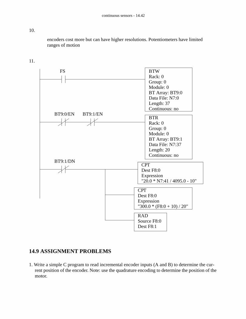
11. A potentiometer is connected to a PLC analog input card. The potentiometer can rotate 300 degrees, and the voltage supply for the potentiometer is +/-10V. Write a ladder logic program to read the voltage from the potentiometer and convert it to an angle in radians stored in F8:0.

14.8 PRACTICE PROBLEM SOLUTIONS

1. Temperature and displacement

2. Sensors can be found at www.ab.com, www.omron.com, etc

3. 360°/64steps, 360°/512steps, 360°/4096steps

4. data bucket, smart machines, PLCs with analog inputs and network connections

5.

Vout α T Tref–( )= 0.030 α 800 Tref–( )= 0.040 α 1000 Tref–( )=

1α---

800 Tref–

0.030------------------------

1000 Tref–

0.040---------------------------= =

800 Tref– 750 0.75Tref–=

50 0.25Tref= Tref 200F= α 0.0401000 200–--------------------------- 50µV

F-------------= =

Vout 0.00005 1200 200–( ) 0.050V= =


6.

7.

8.

9.

a) Vout V2 V1–( )θw

θmax----------- V1+ 5V 0V–( ) 42deg

300deg------------------ 0V+ 0.7V= = =

b) 2.765V 5V 0V–( )θw

300deg------------------ 0V+=

2.765V 5V 0V–( )θw

300deg------------------ 0V+=

θw 165.9deg=

θoutput 0.1deg

count--------------=

θinput

θoutput---------------- 50

1------= θinput 50 0.1

degcount--------------

5deg

count--------------= =

R360

degrot---------

5deg

count--------------

------------------ 72count

rot--------------= =

strain gauge measures strain in a material using a stretching wire that increases resis-tance - accelerometers measure acceleration with a cantilevered mass on a piezoelec-tric element.

+

-

R

DMM V Ksω=

When the motor shaft is turned by another torque source a voltage is gener-ated that is proportional to the angular velocity. This is the reverse emf. A dmm, or other high impedance instrument can be used to measure this, thus minizing the loses in resistor R.

ω· ω K2

JR------ + Vs

KJR------ =

Vs ω K( ) ω· JRK------ +=


10.

11.

14.9 ASSIGNMENT PROBLEMS

1. Write a simple C program to read incremental encoder inputs (A and B) to determine the cur-rent position of the encoder. Note: use the quadrature encoding to determine the position of the motor.

encoders cost more but can have higher resolutions. Potentiometers have limited ranges of motion

BTWRack: 0Group: 0Module: 0BT Array: BT9:0Data File: N7:0Length: 37Continuous: no

FS

BTRRack: 0Group: 0Module: 0BT Array: BT9:1Data File: N7:37Length: 20Continuous: no

BT9:0/EN BT9:1/EN

CPTDest F8:0Expression"20.0 * N7:41 / 4095.0 - 10"

BT9:1/DN

CPTDest F8:0Expression"300.0 * (F8:0 + 10) / 20"

RADSource F8:0Dest F8:1


2. A high precision potentiometer has an accuracy of +/- 0.1% and can rotate 300degrees and is used as a voltage divider with a of 0V and 5V. The output voltage is being read by an A/D con-verter with a 0V to 10V input range. How many bits does the A/D converter need to accommodate the accuracy of the potentiometer?

3. The table of position and voltage values below were measured for an inexpensive potentiome-ter. Write a C subroutine that will accept a voltage value and interpolate the position value.

theta (deg)

067145195213296315

V

0.10.61.62.43.44.25.0

Documents

14. CONTINUOUS SENSORS - Karadimov