14 Competitive Networks 14.1 Hamming Networktmr.meil.pw.edu.pl/web/content/download/5315/26431/file/neural4.pdf · Manukid Parnichkun 195 14 Competitive Networks 14.1 Hamming Network

ASIAN INSTITUTE OF TECHNOLOGY MECHATRONICS

Manukid Parnichkun

195

14 Competitive Networks

14.1 Hamming Network

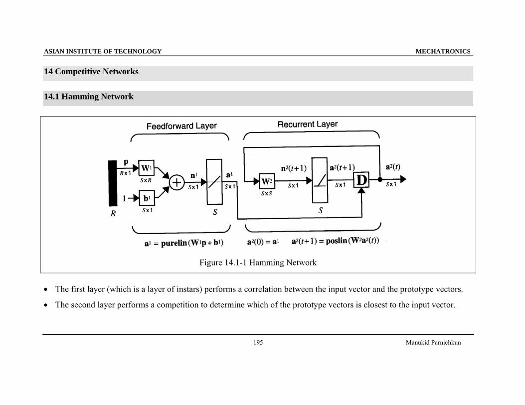
Figure 14.1-1 Hamming Network

• The first layer (which is a layer of instars) performs a correlation between the input vector and the prototype vectors.

• The second layer performs a competition to determine which of the prototype vectors is closest to the input vector.


Manukid Parnichkun

196

Layer 1

• Multiple instars: Multiple pattern recognition

Q Prototype vectors, R: Number of input

},,,{ 21 Qppp K (14.1-1)

⎥⎥⎥⎥

⎦

⎤

⎢⎢⎢⎢

⎣

⎡

=

⎥⎥⎥⎥⎥

⎦

⎤

⎢⎢⎢⎢⎢

⎣

⎡

=

⎥⎥⎥⎥

⎦

⎤

⎢⎢⎢⎢

⎣

⎡

=

R

RR

TQ

T

T

TS

T

T

MMM

12

1

2

1

1 , b

p

pp

w

ww

W (14.1-2)

⎥⎥⎥⎥⎥

⎦

⎤

⎢⎢⎢⎢⎢

⎣

⎡

+

++

=+=

R

RR

TQ

T

T

pp

pppp

bpWaM

2

1

111 (14.1-3)


Manukid Parnichkun

197

Layer 2

• Layer 2: a competitive layer

• Initialized with the outputs of the feedforward layer

• Finally, only one neuron with nonzero output: winning neuron: recognized pattern: a winner-take-all competition 12 )0( aa = (14.1-4)

))(()1( 222 tt aWposlina =+ (14.1-5)

⎩⎨⎧−

=,

,12

εijw otherwise

jiif )( = , where 1

10−

<<S

ε (14.1-6)

⎥⎥⎥⎥

⎦

⎤

⎢⎢⎢⎢

⎣

⎡

−−

−−−−

=

1

11

L

MOMM

L

L

εε

εεεε

W (14.1-7)

⎟⎟⎠

⎞⎜⎜⎝

⎛−=+ ∑

≠ijjii tataposlinta )()()1( 222 ε (14.1-7)

• The output of the neuron with the largest initial condition decreases more slowly than the outputs of the other neurons.


Manukid Parnichkun

198

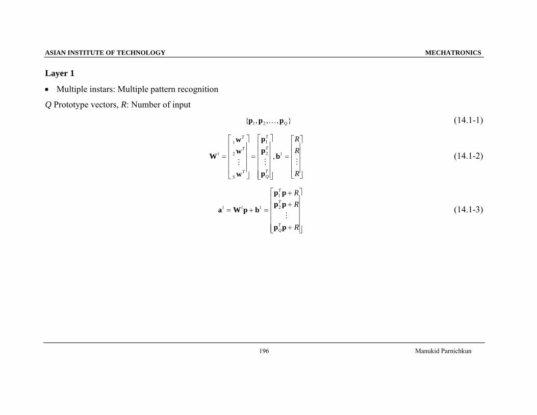
14.2 Competitive Layer

Figure 14.2-1 Competitive Layer

)()( Wpcompetncompeta == (14.2-1)

⎩⎨⎧

≠=

= *

*

,0,1

iiii

ai , where inn ii∀≥ ,* , and *,*

ii nnii =∀≤ (14.2-2)

⎥⎥⎥⎥

⎦

⎤

⎢⎢⎢⎢

⎣

⎡

=

⎥⎥⎥⎥

⎦

⎤

⎢⎢⎢⎢

⎣

⎡

=

⎥⎥⎥⎥

⎦

⎤

⎢⎢⎢⎢

⎣

⎡

==

ST

S

T

T

TS

T

T

L

LL

θ

θθ

cos

coscos

2

22

12

2

1

2

1

MMM

pw

pwpw

p

w

ww

Wpn (14.2-3)


Manukid Parnichkun

199

14.2.1 Competitive Learning

Instar rule,

))1()()(()1()( −−+−= qqqaqq iiii wpww α (14.2.1-1)

Kohonen rule,

)()1()1())1()(()1()( qqqqqq iiii pwwpww ααα +−−=−−+−= (14.2.1-2)

)1()( −= qq ii ww , *ii ≠ (14.2.1-3)

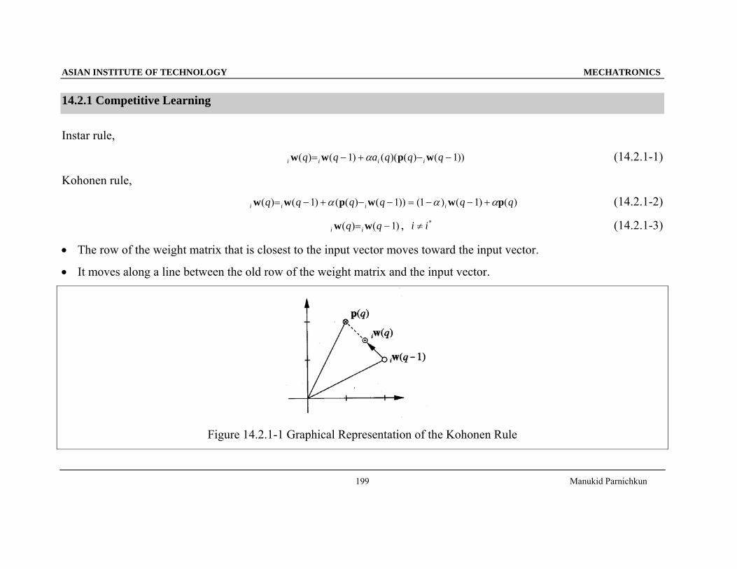
• The row of the weight matrix that is closest to the input vector moves toward the input vector.

• It moves along a line between the old row of the weight matrix and the input vector.

Figure 14.2.1-1 Graphical Representation of the Kohonen Rule


Manukid Parnichkun

200

⎥⎦

⎤⎢⎣

⎡−−

=⎥⎦

⎤⎢⎣

⎡−−

=⎥⎦

⎤⎢⎣

⎡−

=⎥⎦

⎤⎢⎣

⎡=⎥

⎦

⎤⎢⎣

⎡=⎥

⎦

⎤⎢⎣

⎡−=

5812.08137.0

,8137.05812.0

,1961.0

9806.0,

1961.09806.0

,9806.01961.0

,9806.01961.0

654321 pppppp (14.2.1-4)

⎥⎥⎥

⎦

⎤

⎢⎢⎢

⎣

⎡=⎥

⎦

⎤⎢⎣

⎡−=⎥

⎦

⎤⎢⎣

⎡=⎥

⎦

⎤⎢⎣

⎡−

=www

Wwww

3

2

1

321 ,0000.00000.1

,7071.07071.0

,7071.0

7071.0 (14.2.1-5)

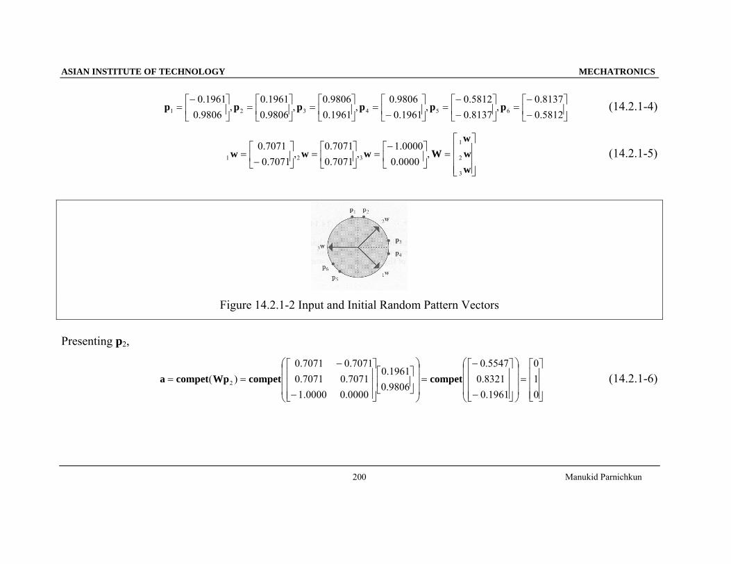
Figure 14.2.1-2 Input and Initial Random Pattern Vectors

Presenting p2,

⎥⎥⎥

⎦

⎤

⎢⎢⎢

⎣

⎡=

⎟⎟⎟

⎠

⎞

⎜⎜⎜

⎝

⎛

⎥⎥⎥

⎦

⎤

⎢⎢⎢

⎣

⎡

−

−=

⎟⎟⎟

⎠

⎞

⎜⎜⎜

⎝

⎛

⎥⎦

⎤⎢⎣

⎡

⎥⎥⎥

⎦

⎤

⎢⎢⎢

⎣

⎡

−

−==

010

1961.08321.05547.0

9806.01961.0

0000.00000.17071.07071.07071.07071.0

)( 2 competcompetWpcompeta (14.2.1-6)


Manukid Parnichkun

201

α = 0.5,

⎥⎦

⎤⎢⎣

⎡=⎟⎟

⎠

⎞⎜⎜⎝

⎛⎥⎦

⎤⎢⎣

⎡−⎥

⎦

⎤⎢⎣

⎡+⎥

⎦

⎤⎢⎣

⎡=−+=

8438.04516.0

7071.07071.0

9806.01961.0

5.07071.07071.0

)( 2222oldoldnew wpww α (14.2.1-7)

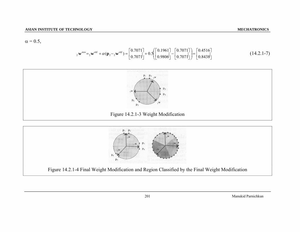
Figure 14.2.1-3 Weight Modification

Figure 14.2.1-4 Final Weight Modification and Region Classified by the Final Weight Modification


Manukid Parnichkun

202

14.2.2 Problems with Competitive Layers

• The choice of learning rate forces a trade-off between the speed of learning and the stability of the final weight vectors.

• When clusters are close together, a weight vector forming a prototype of one cluster may "invade" the territory of

another weight vector.

• A neuron's initial weight vector is located so far from any input vectors that it never wins the competition.

• A competitive layer must have as many classes as it has neurons. When the number of clusters is not known in

advance.

• Competitive layers cannot form classes with nonconvex regions or classes that are the union of unconnected regions.


Manukid Parnichkun

203

14.3 Self Organizing Feature Maps

Kohonen rule,

)()1()1())1()(()1()( qqqqqq iiii pwwpww ααα +−−=−−+−= )(* dNii

∈ (14.3-1)

Neighborhood,

},{)( ddjdN iji ≤= (14.3-2)

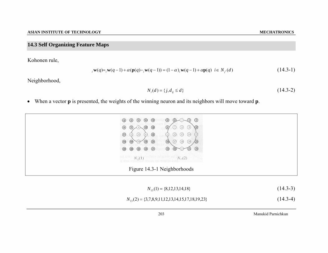
• When a vector p is presented, the weights of the winning neuron and its neighbors will move toward p.

Figure 14.3-1 Neighborhoods

}18,14,13,12,8{)1(13 =N (14.3-3)

}23,19,18,17,15,14,13,12,11,9,8,7,3{)2(13 =N (14.3-4)


Manukid Parnichkun

204

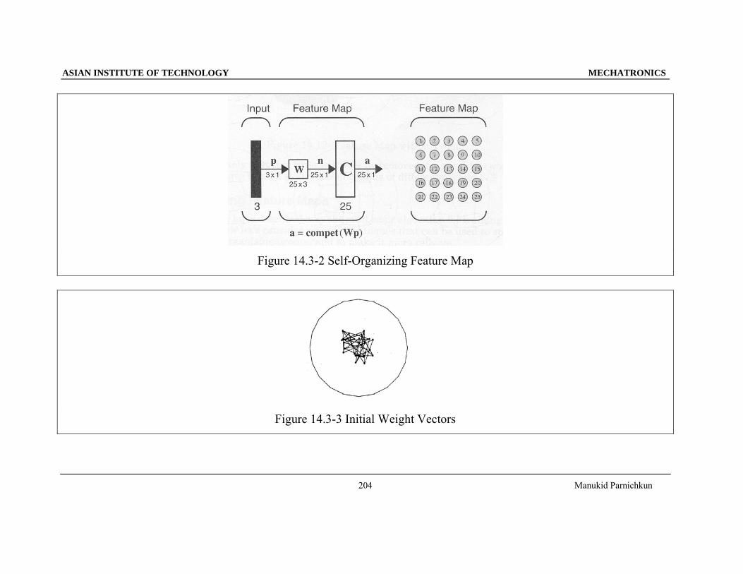
Figure 14.3-2 Self-Organizing Feature Map

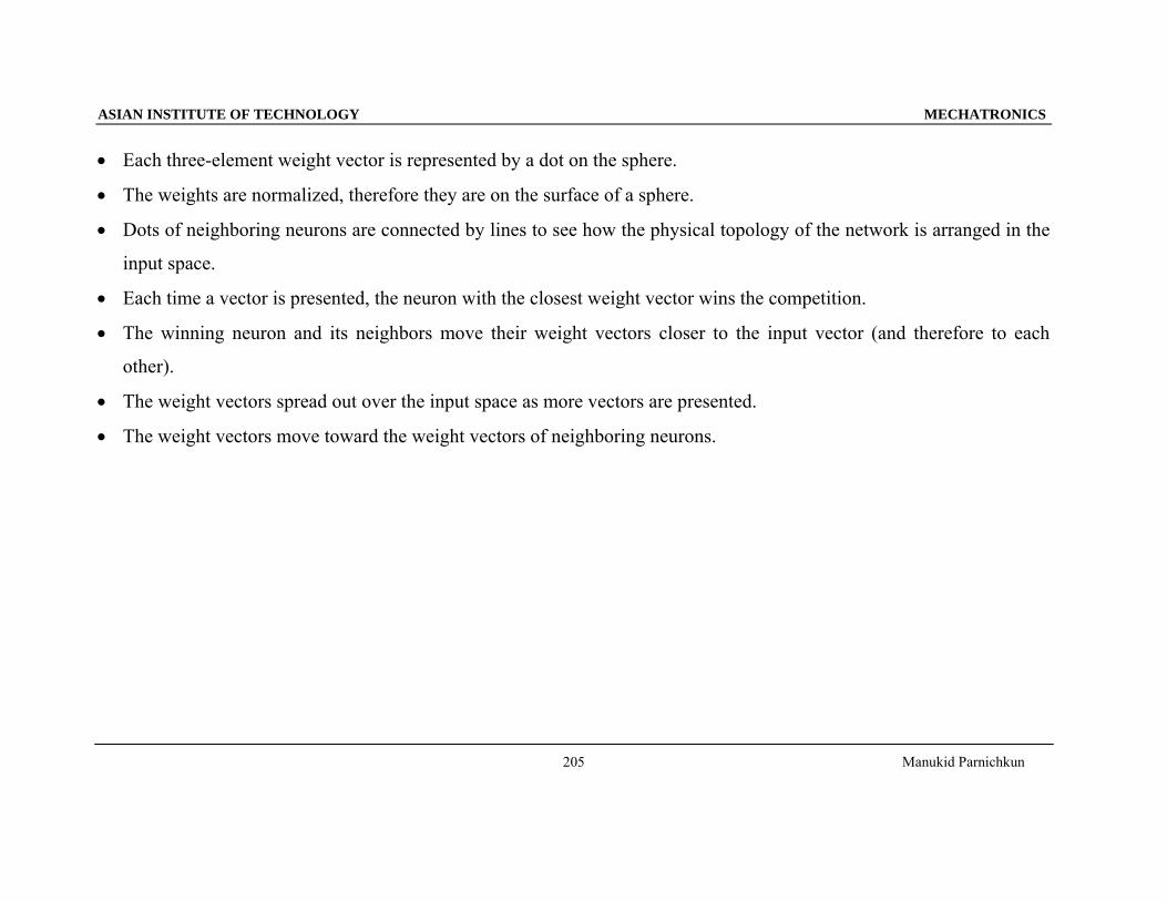
Figure 14.3-3 Initial Weight Vectors


Manukid Parnichkun

205

• Each three-element weight vector is represented by a dot on the sphere.

• The weights are normalized, therefore they are on the surface of a sphere.

• Dots of neighboring neurons are connected by lines to see how the physical topology of the network is arranged in the

input space.

• Each time a vector is presented, the neuron with the closest weight vector wins the competition.

• The winning neuron and its neighbors move their weight vectors closer to the input vector (and therefore to each

other).

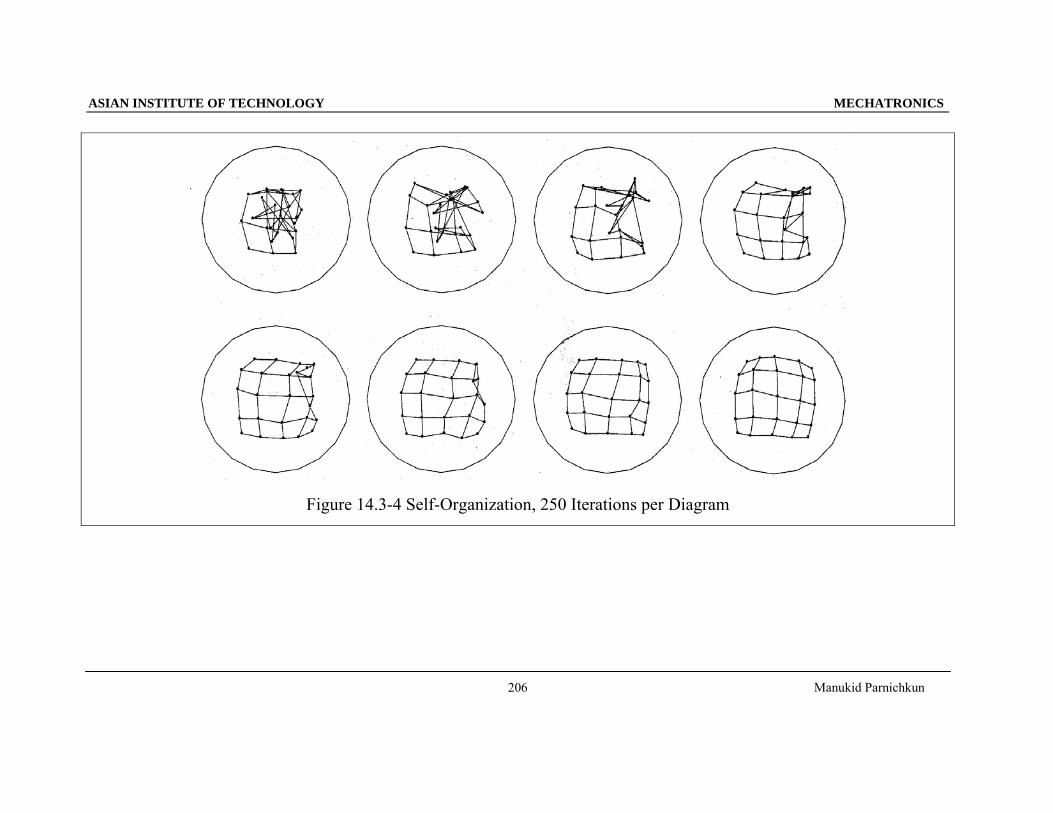
• The weight vectors spread out over the input space as more vectors are presented.

• The weight vectors move toward the weight vectors of neighboring neurons.


Manukid Parnichkun

206

Figure 14.3-4 Self-Organization, 250 Iterations per Diagram


Manukid Parnichkun

207

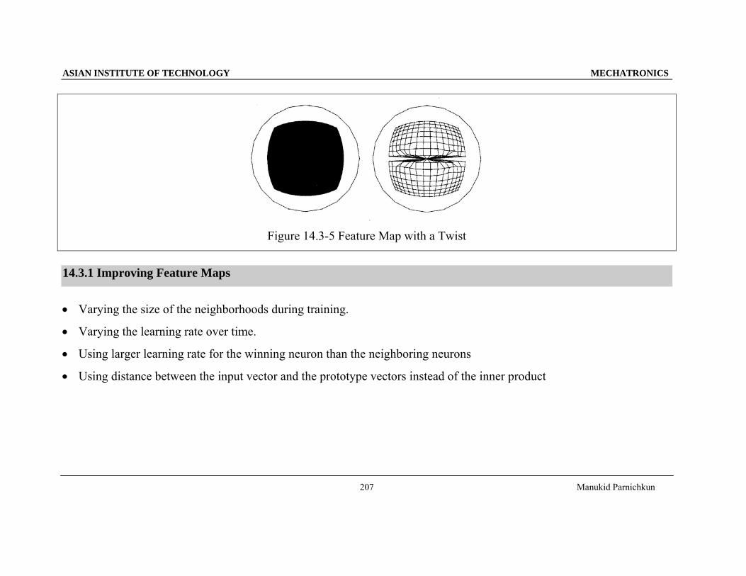
Figure 14.3-5 Feature Map with a Twist

14.3.1 Improving Feature Maps

• Varying the size of the neighborhoods during training.

• Varying the learning rate over time.

• Using larger learning rate for the winning neuron than the neighboring neurons

• Using distance between the input vector and the prototype vectors instead of the inner product


Manukid Parnichkun

208

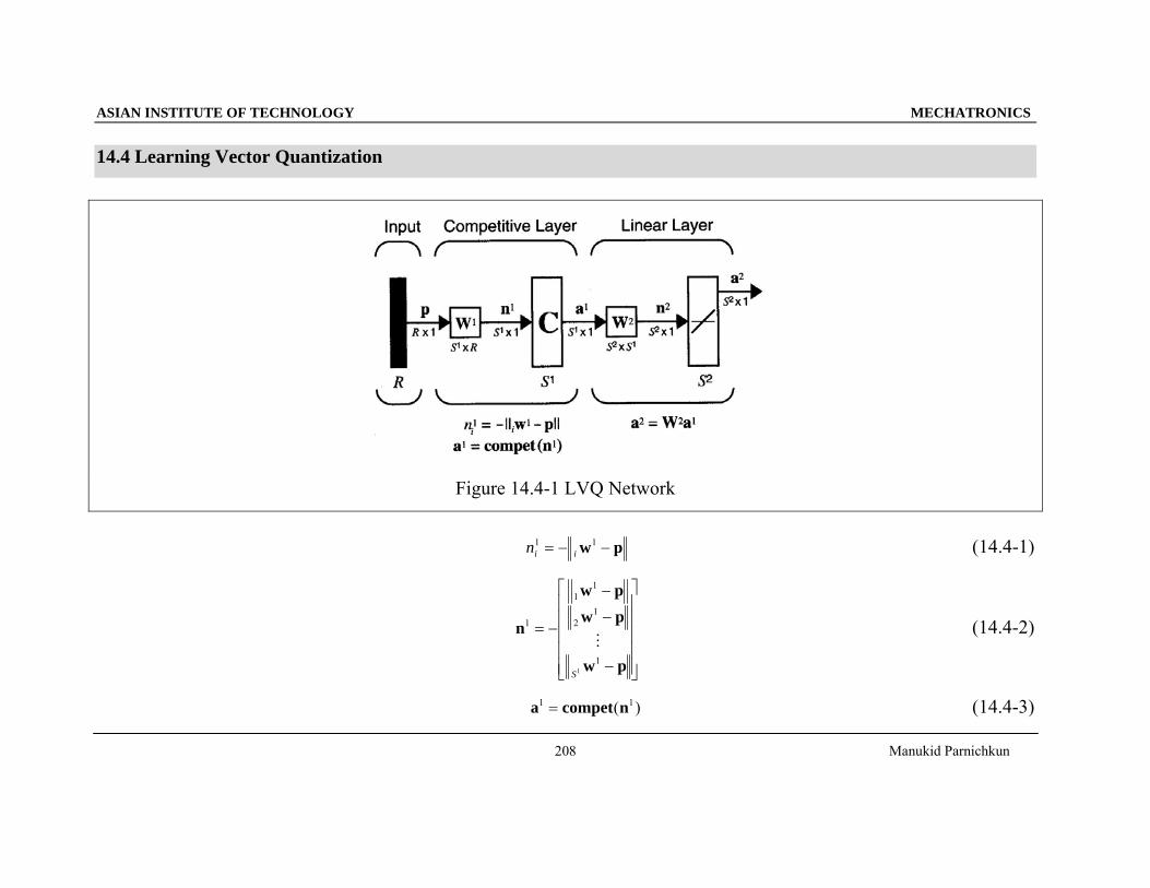
14.4 Learning Vector Quantization

Figure 14.4-1 LVQ Network

pw −−= 11

iin (14.4-1)

⎥⎥⎥⎥⎥

⎦

⎤

⎢⎢⎢⎢⎢

⎣

⎡

−

−

−

−=

pw

pwpw

n

1

12

11

1

1S

M (14.4-2)

)( 11 ncompeta = (14.4-3)


Manukid Parnichkun

209

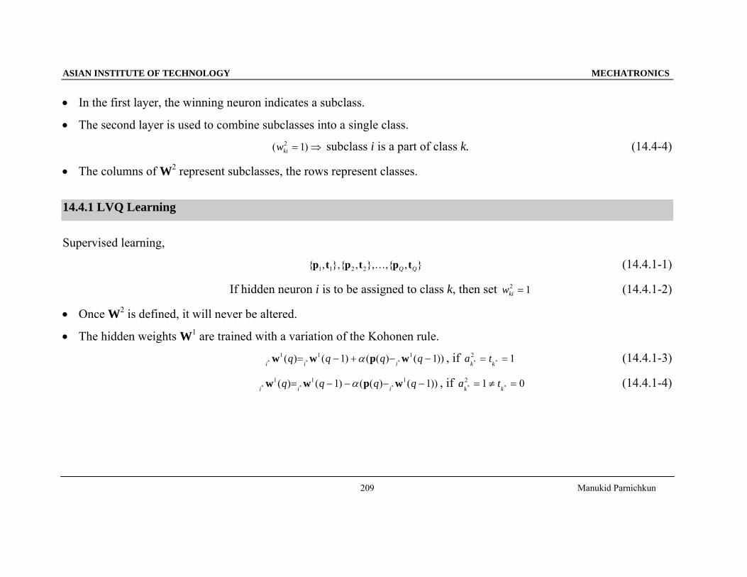
• In the first layer, the winning neuron indicates a subclass.

• The second layer is used to combine subclasses into a single class.

⇒= )1( 2kiw subclass i is a part of class k. (14.4-4)

• The columns of W2 represent subclasses, the rows represent classes.

14.4.1 LVQ Learning

Supervised learning,

},{,},,{},,{ 2211 QQ tptptp K (14.4.1-1)

If hidden neuron i is to be assigned to class k, then set 12 =kiw (14.4.1-2)

• Once W2 is defined, it will never be altered.

• The hidden weights W1 are trained with a variation of the Kohonen rule.

))1()(()1()( 111*** −−+−= qqqq

iiiwpww α , if 1**

2 ==kk

ta (14.4.1-3)

))1()(()1()( 111*** −−−−= qqqq

iiiwpww α , if 01 **

2 =≠=kk

ta (14.4.1-4)


Manukid Parnichkun

210

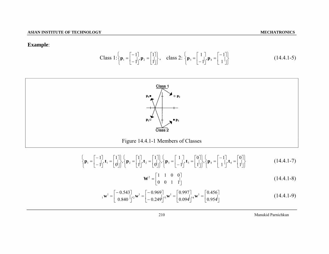
Example:

Class 1:⎭⎬⎫

⎩⎨⎧

⎥⎦

⎤⎢⎣

⎡=⎥

⎦

⎤⎢⎣

⎡−−

=11

,11

21 pp , class 2: ⎭⎬⎫

⎩⎨⎧

⎥⎦

⎤⎢⎣

⎡−=⎥

⎦

⎤⎢⎣

⎡−

=11

,1

143 pp (14.4.1-5)

Figure 14.4.1-1 Members of Classes

⎭⎬⎫

⎩⎨⎧

⎥⎦

⎤⎢⎣

⎡=⎥

⎦

⎤⎢⎣

⎡−=

⎭⎬⎫

⎩⎨⎧

⎥⎦

⎤⎢⎣

⎡=⎥

⎦

⎤⎢⎣

⎡−

=⎭⎬⎫

⎩⎨⎧

⎥⎦

⎤⎢⎣

⎡=⎥

⎦

⎤⎢⎣

⎡=

⎭⎬⎫

⎩⎨⎧

⎥⎦

⎤⎢⎣

⎡=⎥

⎦

⎤⎢⎣

⎡−−

=10

,11

,10

,1

1,

01

,11

,01

,11

44332211 tptptptp (14.4.1-7)

⎥⎦

⎤⎢⎣

⎡=

110000112W (14.4.1-8)

⎥⎦

⎤⎢⎣

⎡=⎥

⎦

⎤⎢⎣

⎡=⎥

⎦

⎤⎢⎣

⎡−−

=⎥⎦

⎤⎢⎣

⎡−=

954.0456.0

,094.0997.0

,249.0969.0

,840.0543.0 1

41

31

21

1 wwww (14.4.1-9)


Manukid Parnichkun

211

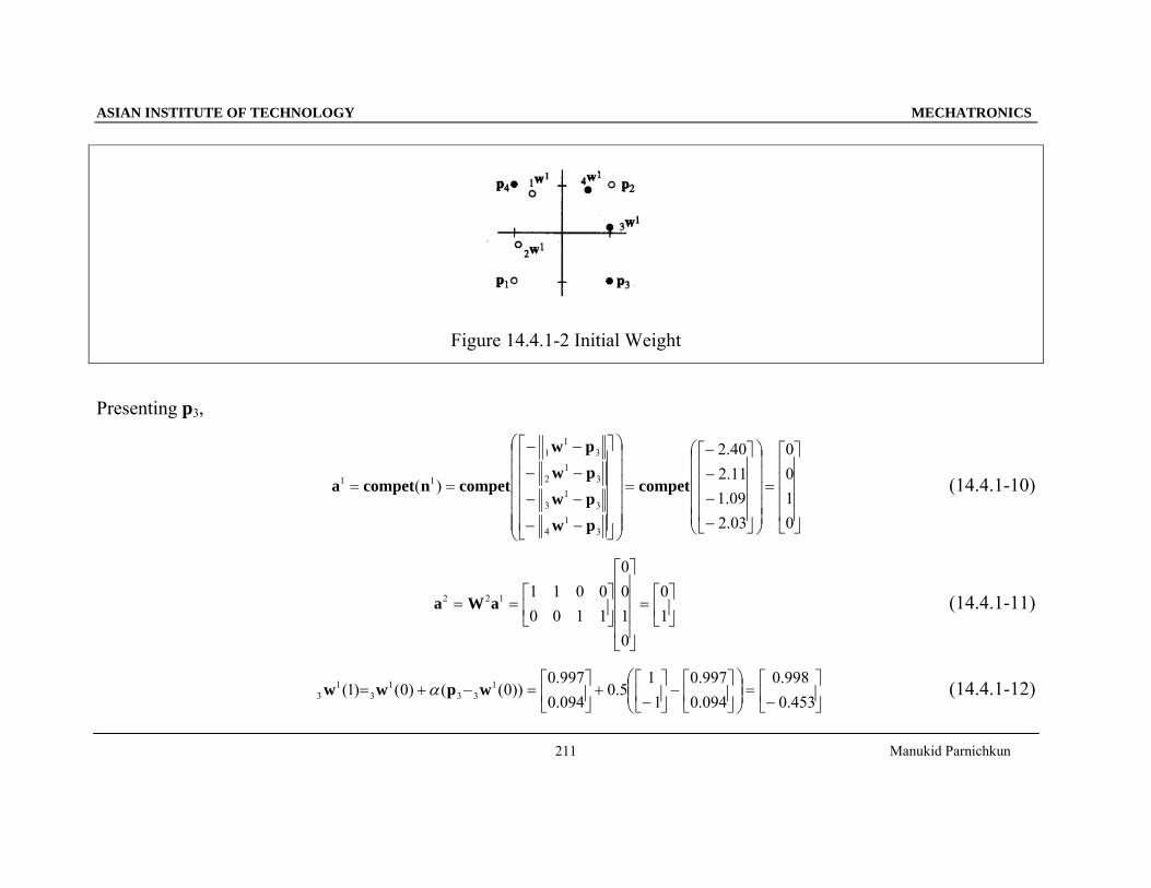
Figure 14.4.1-2 Initial Weight

Presenting p3,

⎥⎥⎥⎥

⎦

⎤

⎢⎢⎢⎢

⎣

⎡

=

⎟⎟⎟⎟⎟

⎠

⎞

⎜⎜⎜⎜⎜

⎝

⎛

⎥⎥⎥⎥

⎦

⎤

⎢⎢⎢⎢

⎣

⎡

−−−−

=

⎟⎟⎟⎟⎟⎟

⎠

⎞

⎜⎜⎜⎜⎜⎜

⎝

⎛

⎥⎥⎥⎥⎥

⎦

⎤

⎢⎢⎢⎢⎢

⎣

⎡

−−

−−

−−

−−

==

0100

03.209.111.240.2

)(

31

4

31

3

31

2

31

1

11 compet

pwpwpwpw

competncompeta (14.4.1-10)

⎥⎦

⎤⎢⎣

⎡=

⎥⎥⎥⎥

⎦

⎤

⎢⎢⎢⎢

⎣

⎡

⎥⎦

⎤⎢⎣

⎡==

10

0100

11000011122 aWa (14.4.1-11)

⎥⎦

⎤⎢⎣

⎡−

=⎟⎟⎠

⎞⎜⎜⎝

⎛⎥⎦

⎤⎢⎣

⎡−⎥

⎦

⎤⎢⎣

⎡−

+⎥⎦

⎤⎢⎣

⎡=−+=

453.0998.0

094.0997.0

11

5.0094.0997.0

))0(()0()1( 133

13

13 wpww α (14.4.1-12)


Manukid Parnichkun

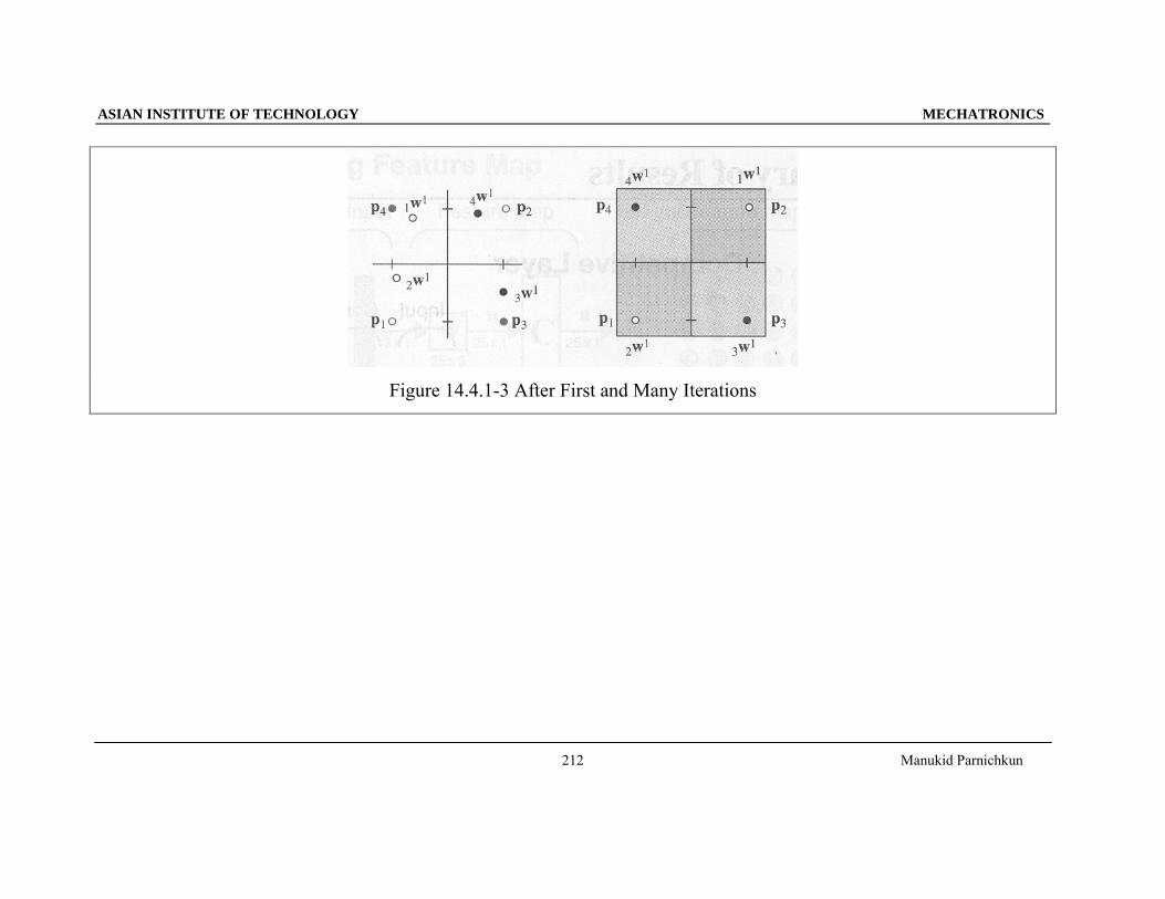
212

Figure 14.4.1-3 After First and Many Iterations


Manukid Parnichkun

213

15 Grossberg Network

15.1 Basic Nonlinear Model

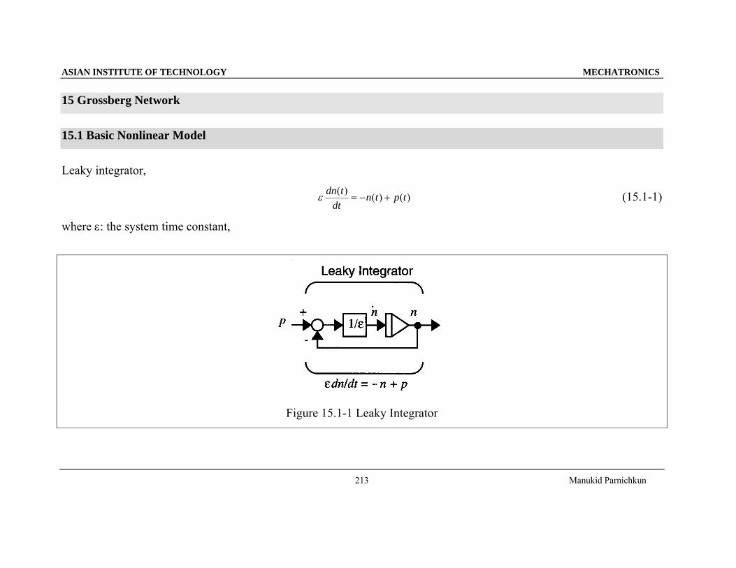
Leaky integrator,

)()()( tptndt

tdn+−=ε (15.1-1)

where ε: the system time constant,

Figure 15.1-1 Leaky Integrator


Manukid Parnichkun

214

The response of the leaky integrator to an arbitrary input p(t),

∫ −+= −−−t

tt dtpenetn0

/)(/ )(1)0()( ττε

ετε (15.1-2)

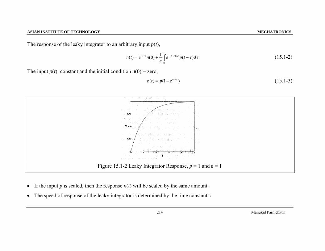
The input p(t): constant and the initial condition n(0) = zero,

)1()( /εteptn −−= (15.1-3)

Figure 15.1-2 Leaky Integrator Response, p = 1 and ε = 1

• If the input p is scaled, then the response n(t) will be scaled by the same amount.

• The speed of response of the leaky integrator is determined by the time constant ε.


Manukid Parnichkun

215

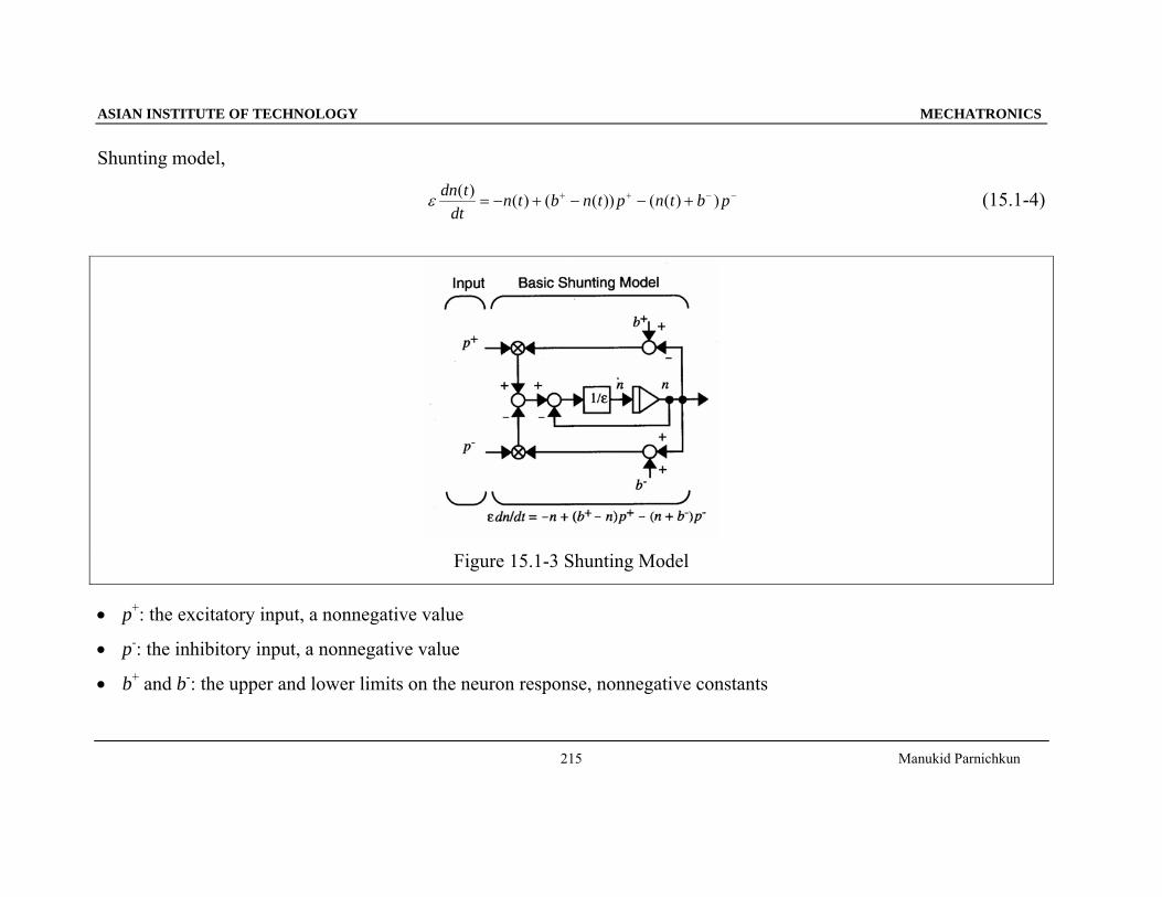
Shunting model,

−−++ +−−+−= pbtnptnbtndt

tdn ))(())(()()(ε (15.1-4)

Figure 15.1-3 Shunting Model

• p+: the excitatory input, a nonnegative value

• p-: the inhibitory input, a nonnegative value

• b+ and b-: the upper and lower limits on the neuron response, nonnegative constants


Manukid Parnichkun

216

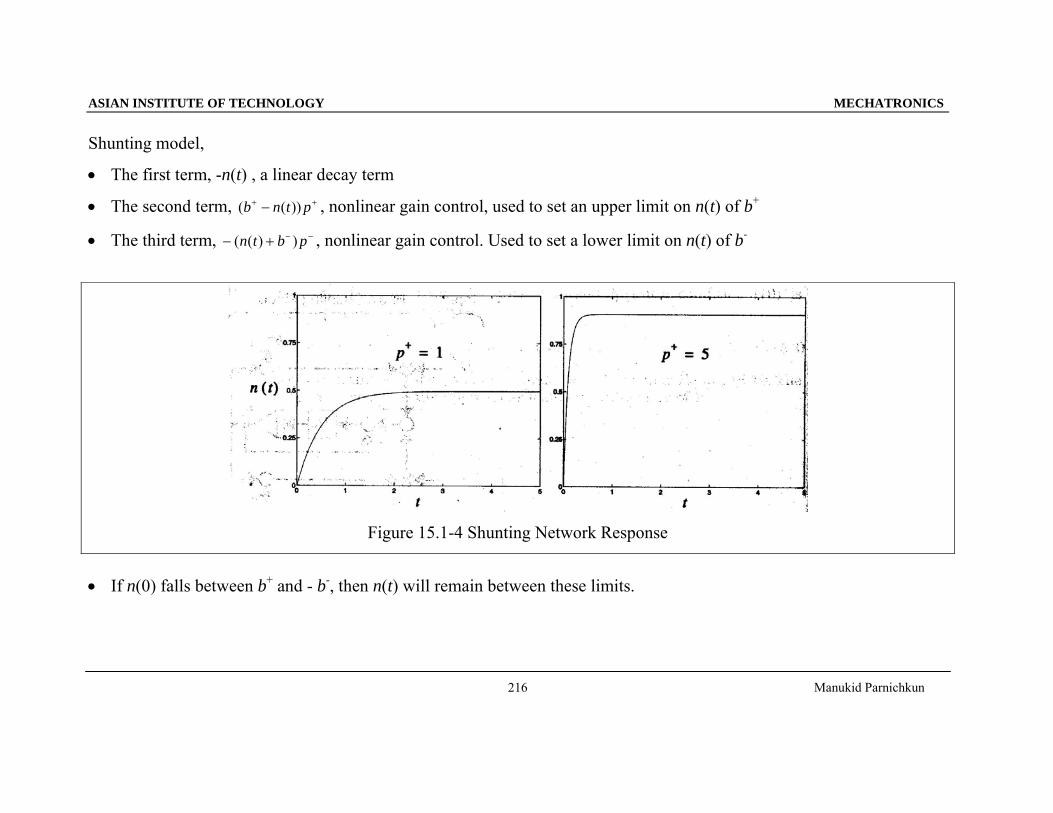
Shunting model,

• The first term, -n(t) , a linear decay term

• The second term, ++ − ptnb ))(( , nonlinear gain control, used to set an upper limit on n(t) of b+

• The third term, −−+− pbtn ))(( , nonlinear gain control. Used to set a lower limit on n(t) of b-

Figure 15.1-4 Shunting Network Response

• If n(0) falls between b+ and - b-, then n(t) will remain between these limits.


Manukid Parnichkun

217

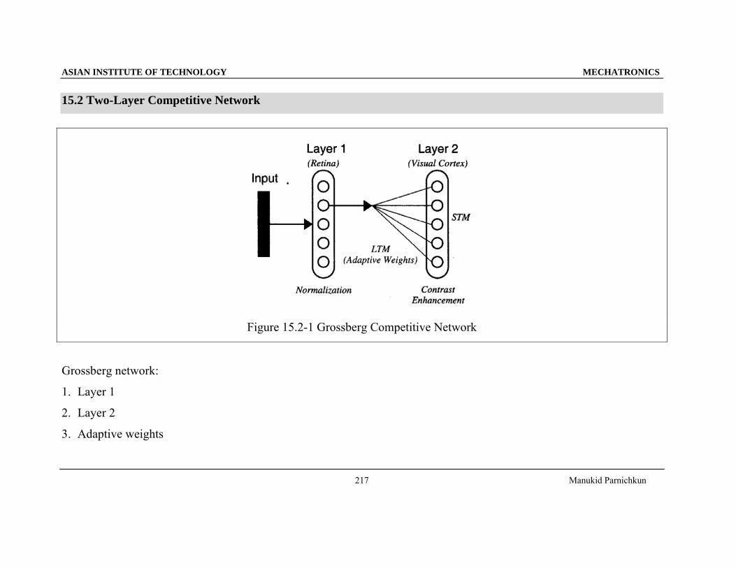
15.2 Two-Layer Competitive Network

Figure 15.2-1 Grossberg Competitive Network

Grossberg network:

1. Layer 1

2. Layer 2

3. Adaptive weights


Manukid Parnichkun

218

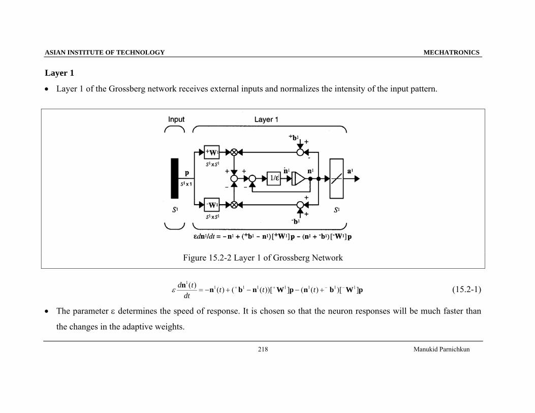
Layer 1

• Layer 1 of the Grossberg network receives external inputs and normalizes the intensity of the input pattern.

Figure 15.2-2 Layer 1 of Grossberg Network

pWbnpWnbnn ])[)((]))[(()()( 11111111

−−++ +−−+−= tttdt

tdε (15.2-1)

• The parameter ε determines the speed of response. It is chosen so that the neuron responses will be much faster than

the changes in the adaptive weights.


Manukid Parnichkun

219

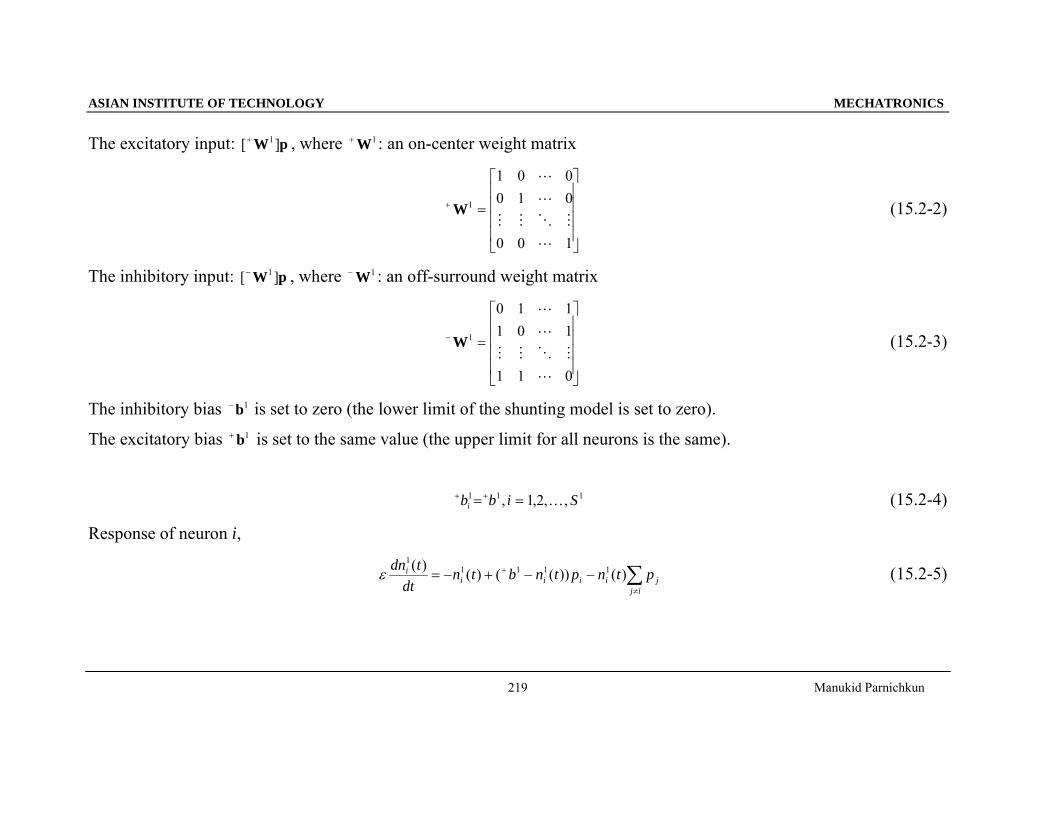
The excitatory input: pW ][ 1+ , where 1W+ : an on-center weight matrix

⎥⎥⎥⎥

⎦

⎤

⎢⎢⎢⎢

⎣

⎡

=+

100

010001

1

L

MOMM

L

L

W (15.2-2)

The inhibitory input: pW ][ 1− , where 1W− : an off-surround weight matrix

⎥⎥⎥⎥

⎦

⎤

⎢⎢⎢⎢

⎣

⎡

=−

011

101110

1

L

MOMM

L

L

W (15.2-3)

The inhibitory bias 1b− is set to zero (the lower limit of the shunting model is set to zero).

The excitatory bias 1b+ is set to the same value (the upper limit for all neurons is the same).

111 ,,2,1, Sibbi K==++ (15.2-4)

Response of neuron i,

∑≠

+ −−+−=ij

jiiiii ptnptnbtndt

tdn )())(()()( 11111

ε (15.2-5)


Manukid Parnichkun

220

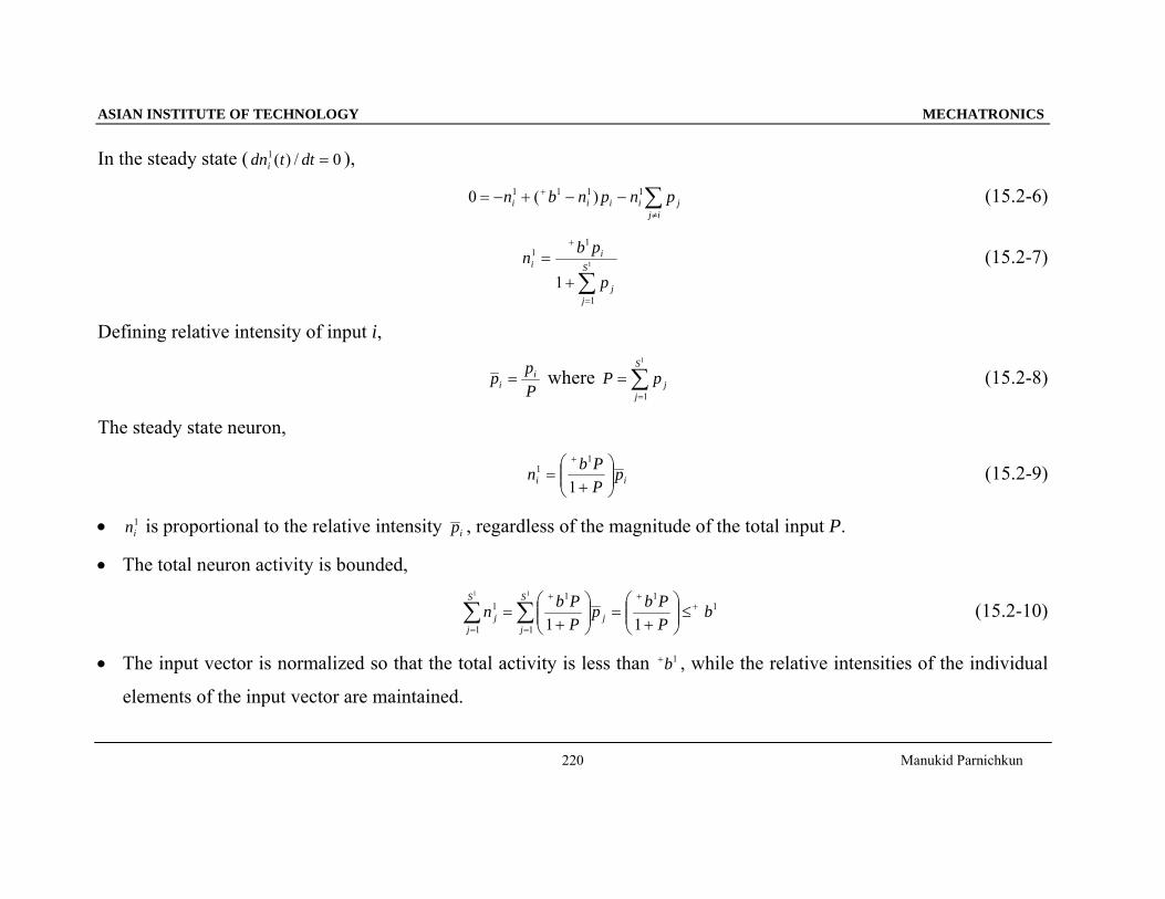
In the steady state ( 0/)(1 =dttdni ),

∑≠

+ −−+−=ij

jiiii pnpnbn 1111 )(0 (15.2-6)

∑=

+

+= 1

1

11

1S

jj

ii

p

pbn (15.2-7)

Defining relative intensity of input i,

Ppp i

i = where ∑=

=1

1

S

jjpP (15.2-8)

The steady state neuron,

ii pPPbn ⎟⎟⎠

⎞⎜⎜⎝

⎛+

=+

1

11 (15.2-9)

• 1in is proportional to the relative intensity ip , regardless of the magnitude of the total input P.

• The total neuron activity is bounded,

1

1 1

111

1 1

11b

PPbp

PPbn

S

j

S

jjj

+

= =

++

≤⎟⎟⎠

⎞⎜⎜⎝

⎛+

=⎟⎟⎠

⎞⎜⎜⎝

⎛+

=∑ ∑ (15.2-10)

• The input vector is normalized so that the total activity is less than 1b+ , while the relative intensities of the individual

elements of the input vector are maintained.


Manukid Parnichkun

221

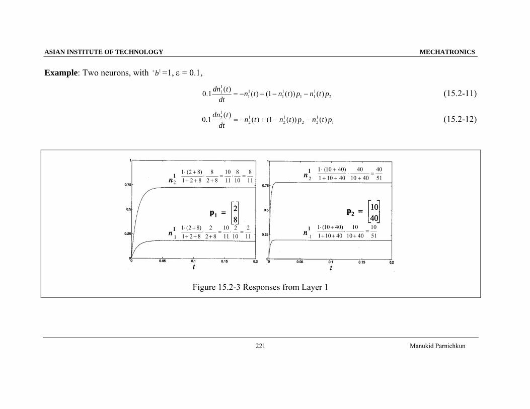
Example: Two neurons, with 1b+ =1, ε = 0.1,

2111

11

11

11 )())(1()()(1.0 ptnptntndt

tdn−−+−= (15.2-11)

1122

12

12

12 )())(1()()(1.0 ptnptntndt

tdn−−+−= (15.2-12)

Figure 15.2-3 Responses from Layer 1

22

1 1

118

108

1110

828

821)82(1

=⋅=+

⋅+++⋅

5140

401040

40101)4010(1

=+

⋅+++⋅

5110

401010

40101)4010(1

=+

⋅+++⋅

112

102

1110

822

821)82(1

=⋅=+

⋅+++⋅


Manukid Parnichkun

222

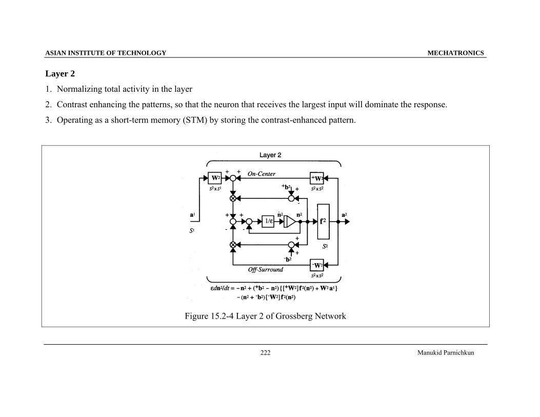
Layer 2

1. Normalizing total activity in the layer

2. Contrast enhancing the patterns, so that the neuron that receives the largest input will dominate the response.

3. Operating as a short-term memory (STM) by storing the contrast-enhanced pattern.

Figure 15.2-4 Layer 2 of Grossberg Network


Manukid Parnichkun

223

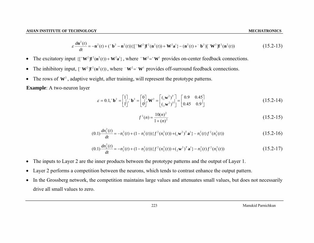
))((])[)((}))((])){[(()()( 22222122222222

tttttdt

td nfWbnaWnfWnbnn −−++ +−+−+−=ε (15.2-13)

• The excitatory input }))((]{[ 12222 aWnfW ++ t , where 12 WW ++ = provides on-center feedback connections.

• The inhibitory input, ))((][ 222 tnfW− , where 12 WW −− = provides off-surround feedback connections.

• The rows of 2W , adaptive weight, after training, will represent the prototype patterns.

Example: A two-neuron layer

⎥⎦

⎤⎢⎣

⎡=⎥

⎦

⎤⎢⎣

⎡=⎥

⎦

⎤⎢⎣

⎡=⎥

⎦

⎤⎢⎣

⎡== −+

9.045.045.09.0

)()(

,00

,11

,1.0 22

21222

T

T

ww

Wbbε (15.2-14)

2

22

)(1)(10)(

nnnf

+= (15.2-15)

))(()(})())(()){(1()()()1.0( 22

221

121

21

221

21

21 tnftntnftntndt

tdn T −+−+−= aw (15.2-16)

))(()(})())(()){(1()()()1.0( 21

222

122

22

222

22

22 tnftntnftntndt

tdn T −+−+−= aw (15.2-17)

• The inputs to Layer 2 are the inner products between the prototype patterns and the output of Layer 1.

• Layer 2 performs a competition between the neurons, which tends to contrast enhance the output pattern.

• In the Grossberg network, the competition maintains large values and attenuates small values, but does not necessarily

drive all small values to zero.


Manukid Parnichkun

224

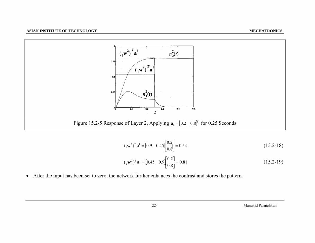
Figure 15.2-5 Response of Layer 2, Applying [ ]T8.02.01 =a for 0.25 Seconds

[ ] 54.08.02.0

45.09.0)( 121 =⎥

⎦

⎤⎢⎣

⎡=aw T (15.2-18)

[ ] 81.08.02.0

9.045.0)( 122 =⎥

⎦

⎤⎢⎣

⎡=aw T (15.2-19)

• After the input has been set to zero, the network further enhances the contrast and stores the pattern.


Manukid Parnichkun

225

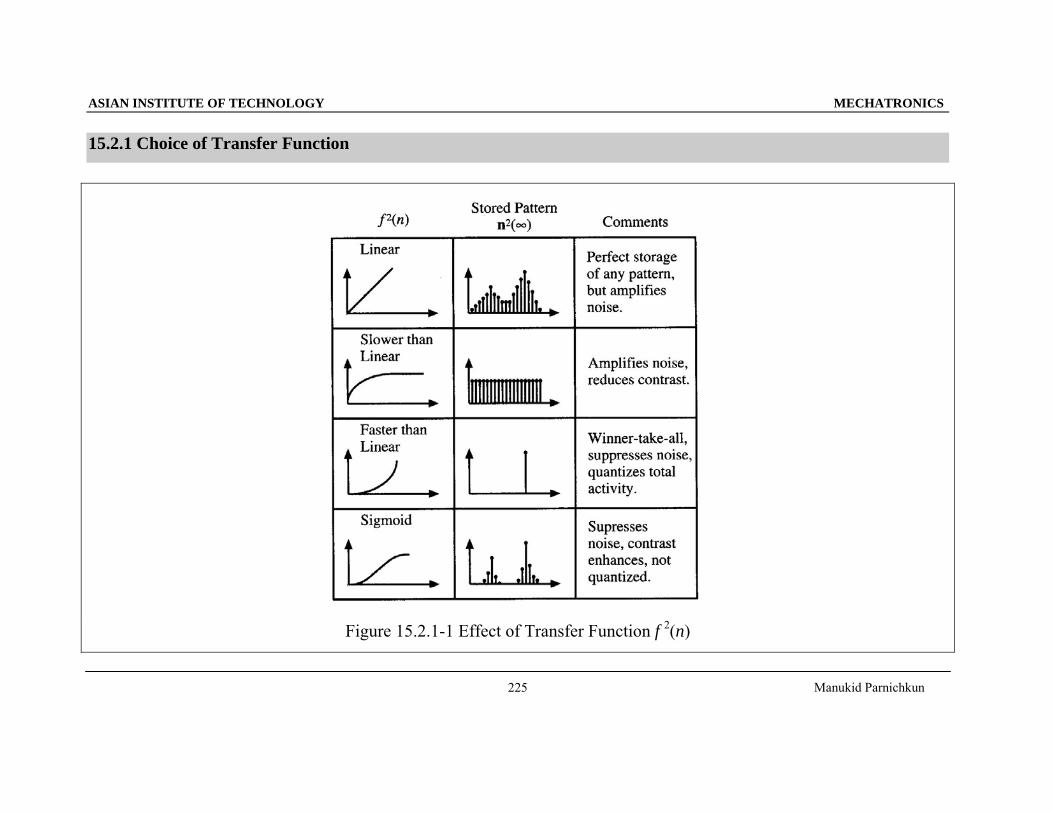
15.2.1 Choice of Transfer Function

Figure 15.2.1-1 Effect of Transfer Function f 2(n)


Manukid Parnichkun

226

15.2.2 Learning Law

• Grossberg calls these adaptive weights, W2, the long-term memory (LTM).

• The rows of W2 represent patterns that have been stored and that the network is be able to recognize.

One learning law for W2,

)}()()({)( 122

,

2, tntntw

dttdw

jijiji +−= α (15.2.2-1)

• The first term is a passive decay term.

• The second term implements a Hebbian-type learning.

• Together, this learning implement the Hebb rule with decay.

Turn off learning when )(2 tni is not active,

)}()(){()( 12

,2

2, tntwtn

dttdw

jjiiji +−= α (15.2.2-2)

)}()]([){()]([ 1222

tttndt

tdii

i nww+−= α (15.2.2-3)

• This is the continuous-time implementation of the instar learning rule.


Manukid Parnichkun

227

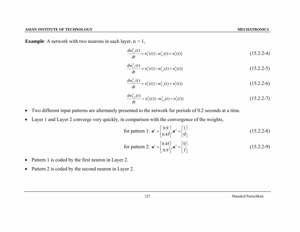
Example: A network with two neurons in each layer, α = 1,

)}()(){()( 1

12

1,121

21,1 tntwtn

dttdw

+−= (15.2.2-4)

)}()(){()( 1

22

2,121

22,1 tntwtn

dttdw

+−= (15.2.2-5)

)}()(){()( 1

12

1,222

21,2 tntwtn

dttdw

+−= (15.2.2-6)

)}()(){()( 1

22

2,222

22,2 tntwtn

dttdw

+−= (15.2.2-7)

• Two different input patterns are alternately presented to the network for periods of 0.2 seconds at a time.

• Layer 1 and Layer 2 converge very quickly, in comparison with the convergence of the weights,

for pattern 1: ⎥⎦

⎤⎢⎣

⎡=⎥

⎦

⎤⎢⎣

⎡=

01

,45.09.0 21 nn (15.2.2-8)

for pattern 2: ⎥⎦

⎤⎢⎣

⎡=⎥

⎦

⎤⎢⎣

⎡=

10

,9.045.0 21 nn (15.2.2-9)

• Pattern 1 is coded by the first neuron in Layer 2.

• Pattern 2 is coded by the second neuron in Layer 2.


Manukid Parnichkun

228

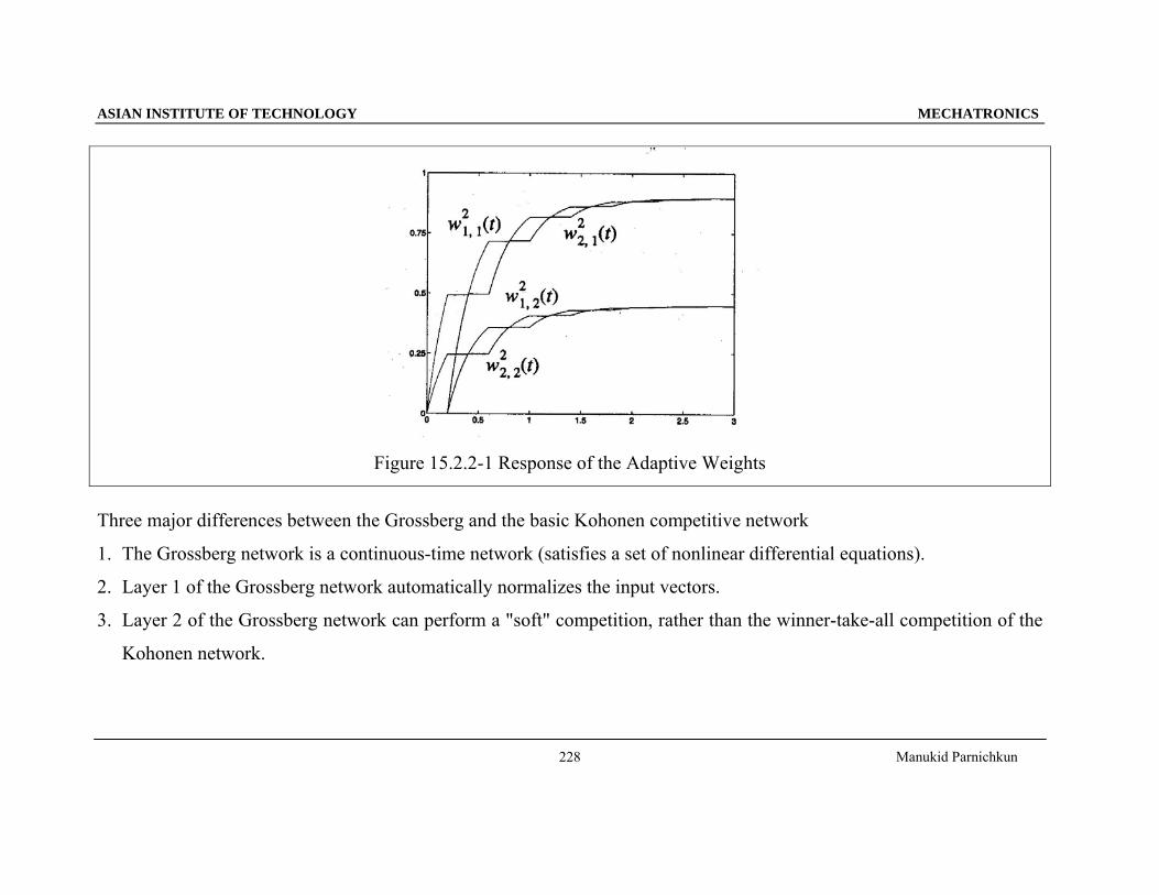
Figure 15.2.2-1 Response of the Adaptive Weights

Three major differences between the Grossberg and the basic Kohonen competitive network

1. The Grossberg network is a continuous-time network (satisfies a set of nonlinear differential equations).

2. Layer 1 of the Grossberg network automatically normalizes the input vectors.

3. Layer 2 of the Grossberg network can perform a "soft" competition, rather than the winner-take-all competition of the

Kohonen network.


Manukid Parnichkun

229

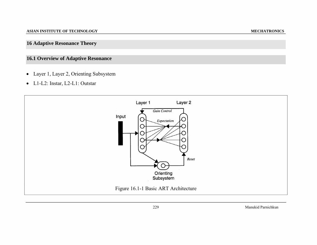
16 Adaptive Resonance Theory

16.1 Overview of Adaptive Resonance

• Layer 1, Layer 2, Orienting Subsystem

• L1-L2: Instar, L2-L1: Outstar

Figure 16.1-1 Basic ART Architecture


Manukid Parnichkun

230

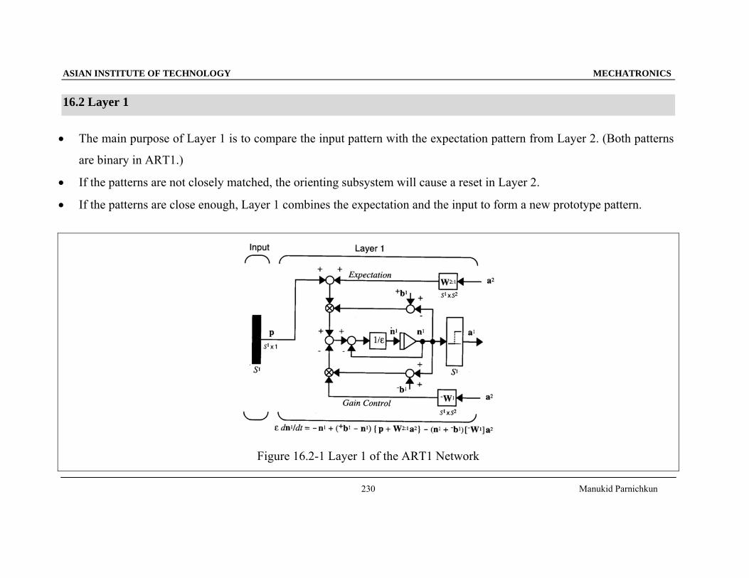
16.2 Layer 1

• The main purpose of Layer 1 is to compare the input pattern with the expectation pattern from Layer 2. (Both patterns

are binary in ART1.)

• If the patterns are not closely matched, the orienting subsystem will cause a reset in Layer 2.

• If the patterns are close enough, Layer 1 combines the expectation and the input to form a new prototype pattern.

Figure 16.2-1 Layer 1 of the ART1 Network


Manukid Parnichkun

231

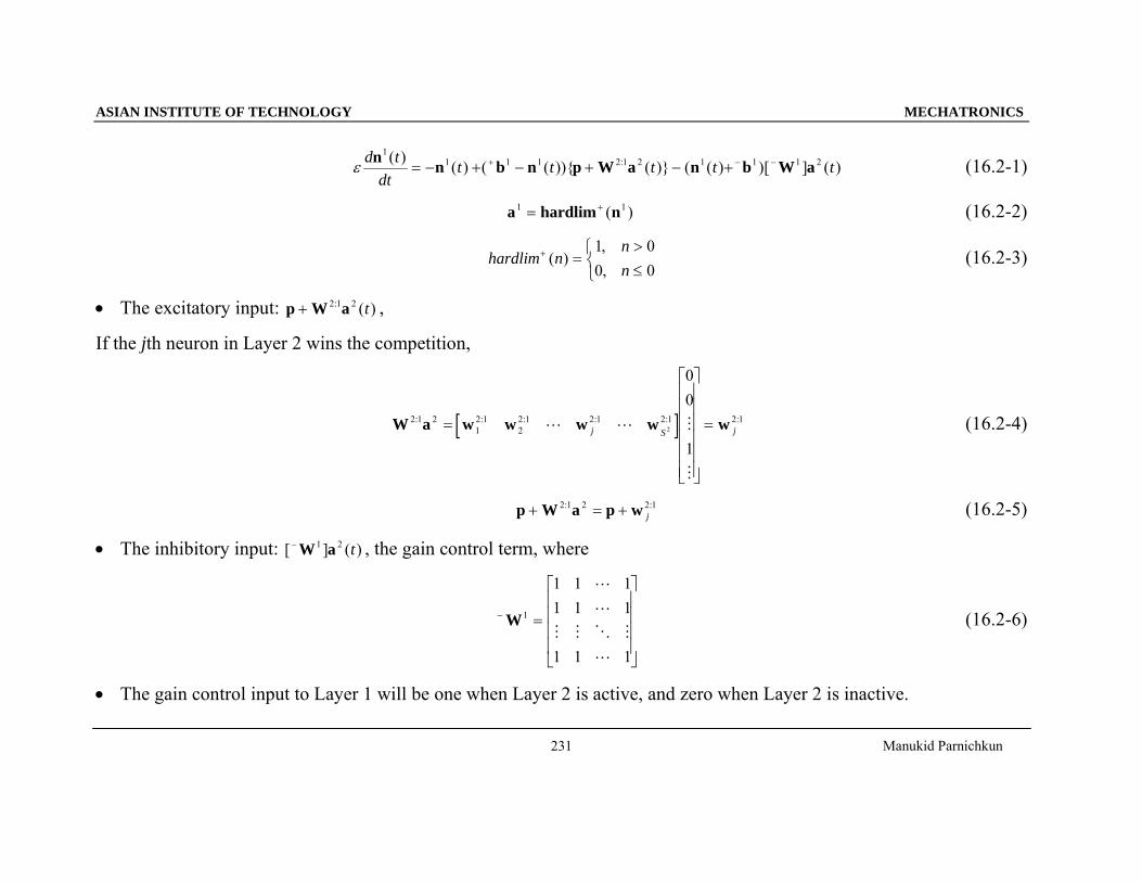
ε d tdt

t t t t tn n b n p W a n b W a1

1 1 1 2 1 2 1 1 1 2( ) ( ) ( ( )){ ( )} ( ( ) )[ ] ( ):= − + − + − ++ − − (16.2-1)

a hardlim n1 1= + ( ) (16.2-2)

hardlim n+ =⎧⎨⎩

( ),,

10

nn>≤

00

(16.2-3)

• The excitatory input: p W a+ 2 1 2: ( )t ,

If the jth neuron in Layer 2 wins the competition,

[ ]W a w w w w w2 1 212 1

22 1 2 1 2 1 2 1

2

00

1

: : : : : :=

⎡

⎣

⎢⎢⎢⎢⎢⎢

⎤

⎦

⎥⎥⎥⎥⎥⎥

=L L M

M

j S j (16.2-4)

p W a p w+ = +2 1 2 2 1: :j (16.2-5)

• The inhibitory input: [ ] ( )−W a1 2 t , the gain control term, where

− =

⎡

⎣

⎢⎢⎢⎢

⎤

⎦

⎥⎥⎥⎥

W1

1 1 11 1 1

1 1 1

L

L

M M O M

L

(16.2-6)

• The gain control input to Layer 1 will be one when Layer 2 is active, and zero when Layer 2 is inactive.


Manukid Parnichkun

232

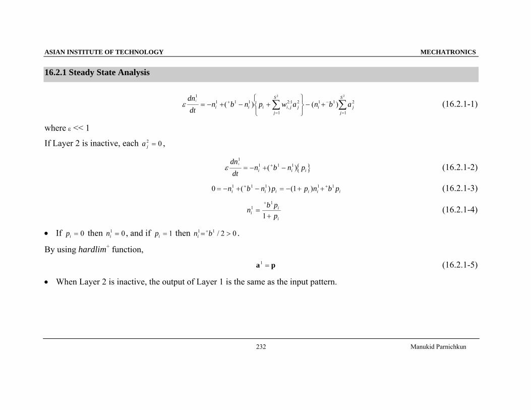
16.2.1 Steady State Analysis

εdndt

n b n p w a n b ai

i i i i j jj

S

i jj

S11 1 1 2 1 2

1

1 1 2

1

2 2

= − + − +⎧⎨⎩

⎫⎬⎭− ++

=

−

=∑ ∑( ) ( ),

: (16.2.1-1)

where ε << 1

If Layer 2 is inactive, each a j2 0= ,

{ }εdndt

n b n pi

i i i

11 1 1= − + −+( ) (16.2.1-2)

0 11 1 1 1 1= − + − = − + ++ +n b n p p n b pi i i i i i( ) ( ) (16.2.1-3)

n b ppi

i

i

11

1=

+

+

(16.2.1-4)

• If pi = 0 then ni1 0= , and if pi = 1 then n bi

1 1 2 0= >+ / .

By using hardlim+ function,

a p1 = (16.2.1-5)

• When Layer 2 is inactive, the output of Layer 1 is the same as the input pattern.


Manukid Parnichkun

233

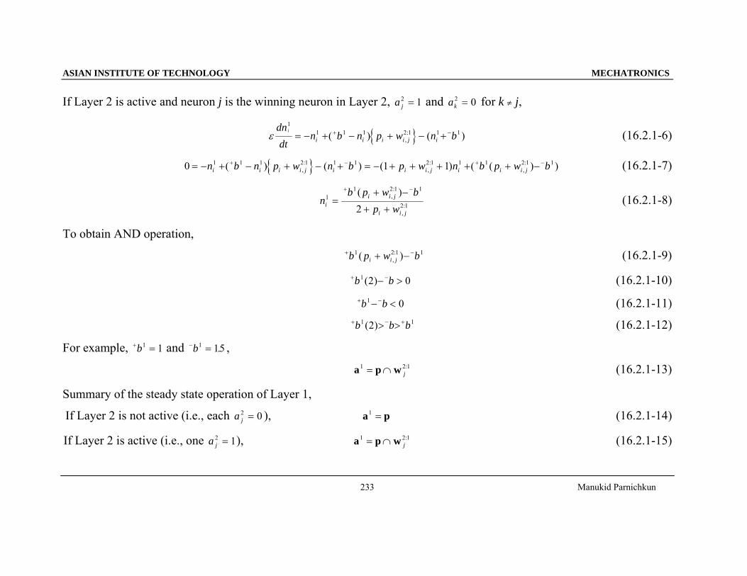
If Layer 2 is active and neuron j is the winning neuron in Layer 2, a j

2 1= and ak2 0= for k ≠ j,

{ }εdndt

n b n p w n bi

i i i i j i

11 1 1 2 1 1 1= − + − + − ++ −( ) ( ),

: (16.2.1-6)

{ }0 1 11 1 1 2 1 1 1 2 1 1 1 2 1 1= − + − + − + = − + + + + + −+ − + −n b n p w n b p w n b p w bi i i i j i i i j i i i j( ) ( ) ( ) ( ( ) ),:

,:

,: (16.2.1-7)

nb p w b

p wii i j

i i j

11 2 1 1

2 12=

+ −

+ +

+ −( ),:

,: (16.2.1-8)

To obtain AND operation, + −+ −b p w bi i j

1 2 1 1( ),: (16.2.1-9)

+ −− >b b1 2 0( ) (16.2.1-10) + −− <b b1 0 (16.2.1-11)

+ − +> >b b b1 12( ) (16.2.1-12)

For example, + =b1 1 and − =b1 15. ,

a p w1 2 1= ∩ j: (16.2.1-13)

Summary of the steady state operation of Layer 1,

If Layer 2 is not active (i.e., each a j2 0= ), a p1 = (16.2.1-14)

If Layer 2 is active (i.e., one a j2 1= ), a p w1 2 1= ∩ j

: (16.2.1-15)


Manukid Parnichkun

234

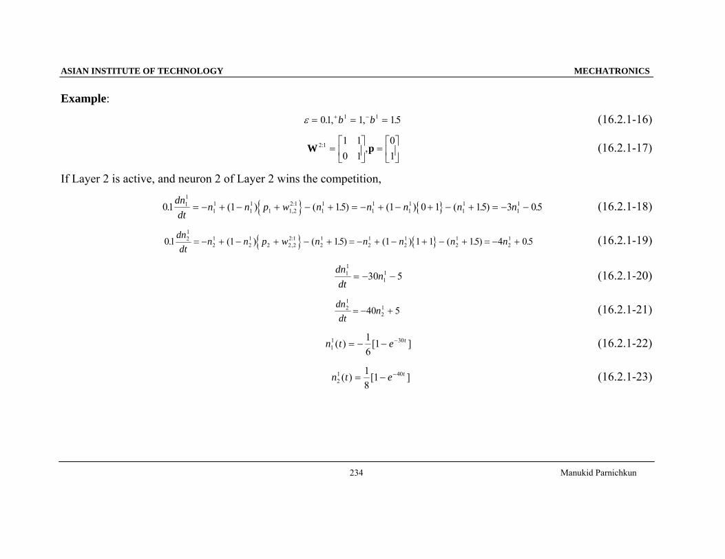
Example:

ε = = =+ −01 1 151 1. , , .b b (16.2.1-16)

W p2 1 1 10 1

01

: ,=⎡

⎣⎢

⎤

⎦⎥ =

⎡

⎣⎢⎤

⎦⎥ (16.2.1-17)

If Layer 2 is active, and neuron 2 of Layer 2 wins the competition,

{ } { }01 1 15 1 0 1 15 3 0511

11

11

1 1 22 1

11

11

11

11

11. ( ) ( . ) ( ) ( . ) .,

:dndt

n n p w n n n n n= − + − + − + = − + − + − + = − − (16.2.1-18)

{ } { }01 1 15 1 1 1 15 4 0521

21

21

2 2 22 1

21

21

21

21

21. ( ) ( . ) ( ) ( . ) .,

:dndt

n n p w n n n n n= − + − + − + = − + − + − + = − + (16.2.1-19)

dndt

n11

1130 5= − − (16.2.1-20)

dndt

n21

2140 5= − + (16.2.1-21)

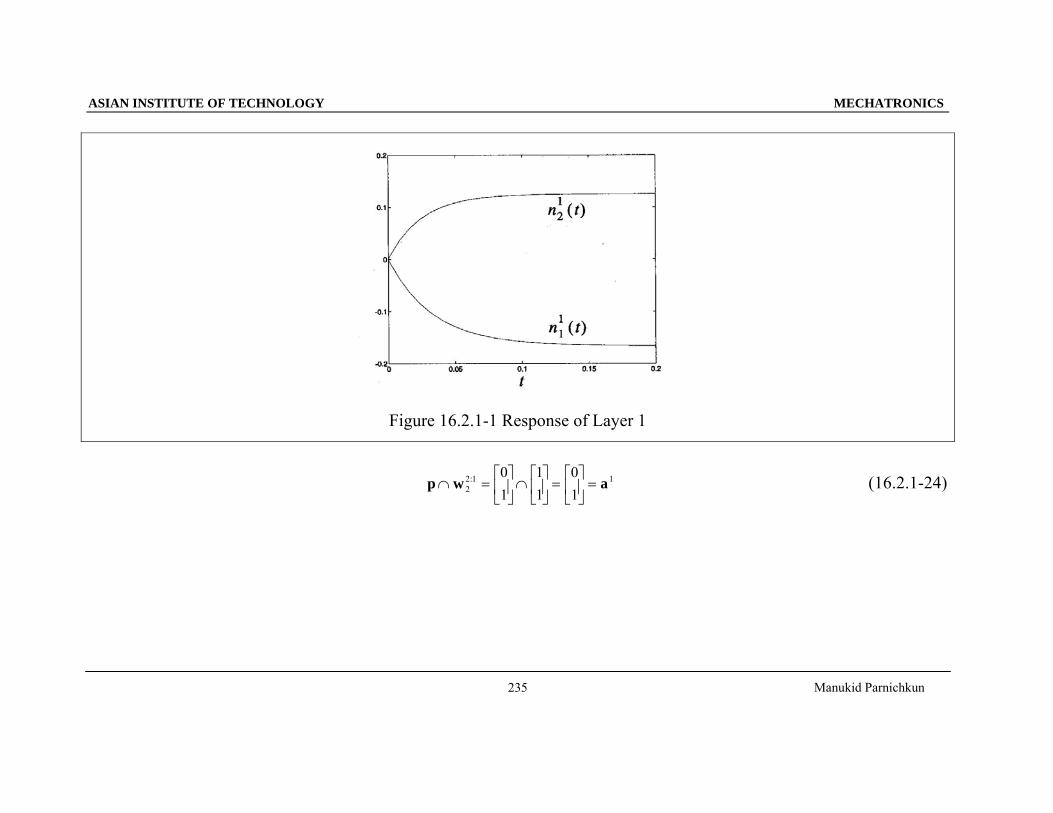
n t e t11 301

61( ) [ ]= − − − (16.2.1-22)

n t e t21 401

81( ) [ ]= − − (16.2.1-23)


Manukid Parnichkun

235

Figure 16.2.1-1 Response of Layer 1

p w a∩ =⎡

⎣⎢⎤

⎦⎥ ∩

⎡

⎣⎢⎤

⎦⎥ =

⎡

⎣⎢⎤

⎦⎥ =2

2 1 101

11

01

: (16.2.1-24)


Manukid Parnichkun

236

16.3 Layer 2

• Layer 2 of the ART1 network is almost identical to Layer 2 of the Grossberg network.

• Its main purpose is to contrast enhance its output pattern, winner-take-all competition.

• The integrator of ART can be reset.

• In this type of integrator any positive outputs are reset to zero whenever the a 0 signal becomes positive.

• The outputs that are reset remain inhibited for a long period of time until an adequate match has occurred and the

weights have been updated.

• The reset signal, a 0 , is the output of the orienting subsystem. It generates a reset whenever there is a mismatch at

Layer 1 between the input signal and the L2-L1 expectation.

• Two transfer functions are used in ART1.

• The transfer function f2(n2) is used for the on-center/off-surround feedback connections.

• The output of Layer 2 is computed as a2 = hardlim+(n2) .


Manukid Parnichkun

237

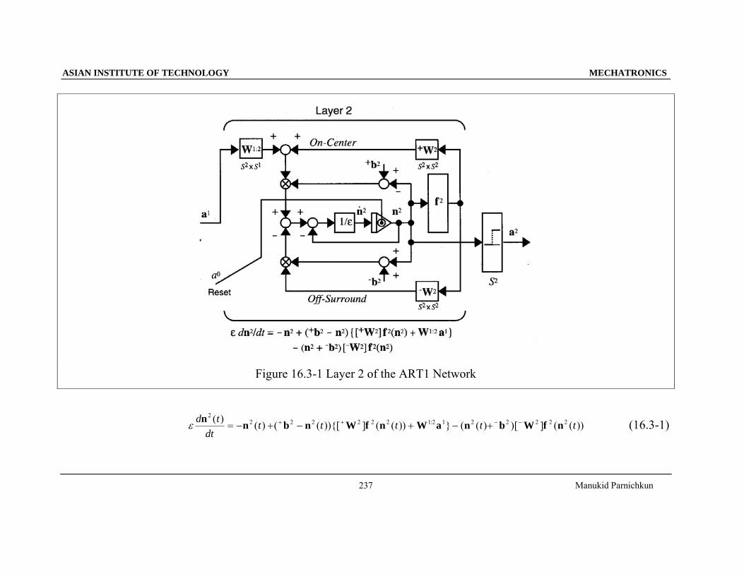
Figure 16.3-1 Layer 2 of the ART1 Network

ε d tdt

t t t t tn n b n W f n W a n b W f n2

2 2 2 2 2 2 1 2 1 2 2 2 2 2( ) ( ) ( ( )){[ ] ( ( )) } ( ( ) )[ ] ( ( )):= − + − + − ++ + − − (16.3-1)


Manukid Parnichkun

238

The excitatory input: {[ ] ( ( )) }:+ +W f n W a2 2 2 1 2 1t + W 2 : on-center feedback connections

W1 2: : adaptive weights, trained according to an instar rule

The inhibitory input: [ ] ( ( ))− W f n2 2 2 t − W 2 : off-surround feedback connections

Example: A two-neuron layer,

ε = =⎡

⎣⎢⎤

⎦⎥ =

⎡

⎣⎢⎤

⎦⎥ =

⎡

⎣⎢

⎤

⎦⎥ =

⎡

⎣⎢

⎤

⎦⎥

+ −0111

11

0 5 0 51 0

2 2 1 2 11 2

21 2. , , ,

( )( )

. .::

:b b Www

T

T (16.3-2)

f nn2

2100

( )( ) ,

,=⎧⎨⎩

nn≥<

00

(16.3-3)

( . )( )

( ) ( ( )){ ( ( )) ( ) } ( ( ) ) ( ( )):01 1 112

12

12 2

12

11 2 1

12 2

22dn t

dtn t n t f n t n t f n tT= − + − + − +w a (16.3-4)

( . ) ( ) ( ) ( ( )){ ( ( )) ( ) } ( ( ) ) ( ( )):01 1 122

22

22 2

22

21 2 1

22 2

12dn t

dtn t n t f n t n t f n tT= − + − + − +w a (16.3-5)

• The inputs to Layer 2 are the inner products of the prototype patterns with the output of Layer 1.

• Layer 2 then performs a competition between the neurons.

• The transfer function f2(n) is chosen to be a faster-than-linear transfer function.

• After the competition, one neuron output will be 1, and the other neuron output will be zero.


Manukid Parnichkun

239

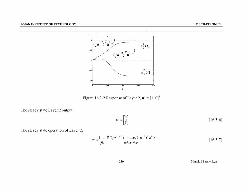
Figure 16.3-2 Response of Layer 2, a1 = [1 0]T

The steady state Layer 2 output,

a 2 01

=⎡

⎣⎢⎤

⎦⎥ (16.3-6)

The steady state operation of Layer 2,

ai2 1

0=⎧⎨⎩

,, if

otherwisei

Tj

T(( ) max[( ) ]): :w a w a1 2 1 1 2 1= (16.3-7)


Manukid Parnichkun

240

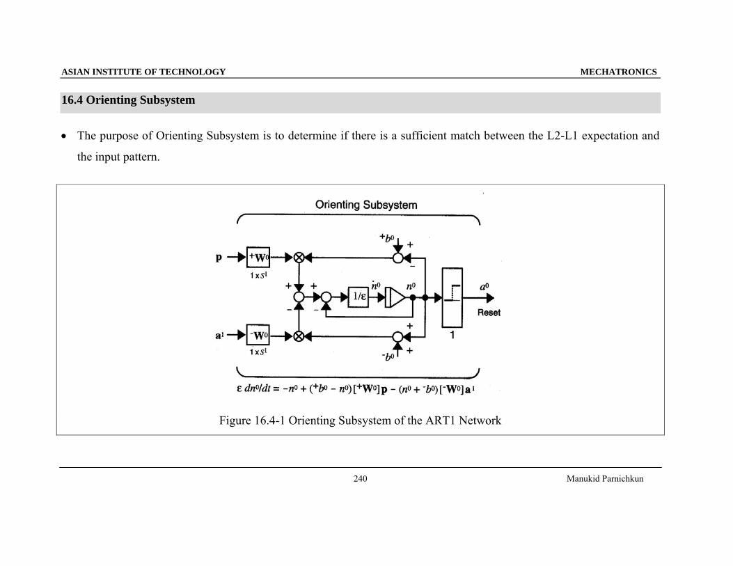
16.4 Orienting Subsystem

• The purpose of Orienting Subsystem is to determine if there is a sufficient match between the L2-L1 expectation and

the input pattern.

Figure 16.4-1 Orienting Subsystem of the ART1 Network


Manukid Parnichkun

241

ε dn tdt

n t b n t n t b0

0 0 0 0 0 0 0 1( ) ( ) ( ( )){ } ( ( ) ){ }= − + − − ++ + − −W p W a (16.4-1)

The excitatory input: + W p0 , where

[ ]+ =W 0 α α αL (16.4-2)

[ ]+

=

= = =∑W p p p0 2

1

1

α α α α αL p jj

S

(16.4-3)

The inhibitory input: − W a0 1 , where

[ ]− =W 0 β β βL (16.4-4)

[ ]−

=

= = =∑W a a a0 1 1 1 1 2

1

1

β β β β βL a tjj

S

( ) (16.4-5)

0 10 0 0 2 0 0 1 2 2 1 2 0 0 2 0 1 2= − + − − + = − + + + −+ − + −n b n n b n b b( ){ } ( ){ } ( ) ( ) ( )α β α β α βp a p a p a (16.4-6)

nb b

n0

0 2 0 1 2

2 1 2 01=

−

+ +

+ −( ) ( )

( )

α β

α β

p a

p a (16.4-7)

+ −= =b b0 0 1 , then n0 > 0 if α βp a2 1 20− > ,

n if01 2

20> < =,a

pαβ

ρ (16.4-8)


Manukid Parnichkun

242

ρ: vigilance parameter, 0 < ρ < 1

If the vigilance is close to 1, a reset will occur unless a1 is close to p.

If the vigilance is close to 0, a1 need not be close to p to prevent a reset.

Eample:

ε α β ρ= = = =01 3 4 0 75. , , , ( . )or (16.4-9)

p a=⎡

⎣⎢⎤

⎦⎥ =

⎡

⎣⎢⎤

⎦⎥

11

10

1, (16.4-10)

( . ) ( ) ( ) ( ( )){ ( )} ( ( ) ){ ( )}01 1 3 1 40

0 01 2

011

21dn t

dtn t n t p p n t a a= − + − + − + + (16.4-11)

dn tdt

n t0

0110 20( ) ( )= − + (16.4-12)


Manukid Parnichkun

243

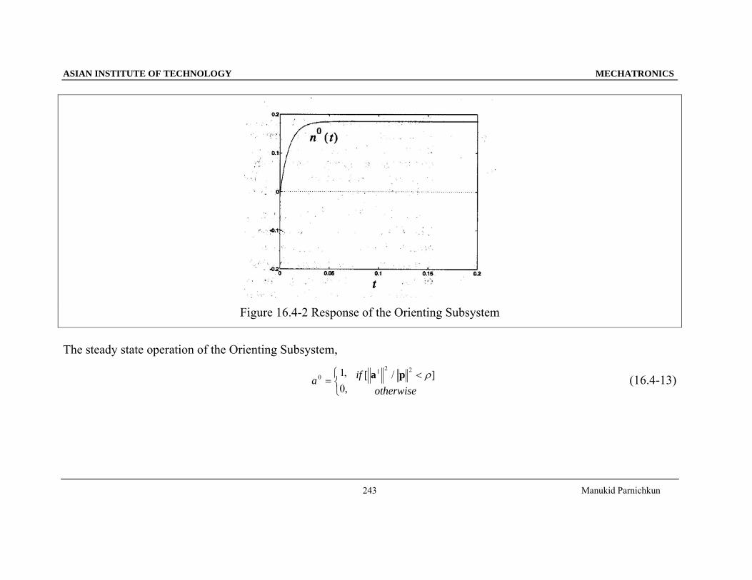
Figure 16.4-2 Response of the Orienting Subsystem

The steady state operation of the Orienting Subsystem,

a 0 10

=⎧⎨⎩

,, if

otherwise[ / ]a p1 2 2 < ρ (16.4-13)


Manukid Parnichkun

244

16.5 Learning Law: Ll-L2

16.5.2 Learning Law: L1-L2

Learning law for W1:2,

[ ])(]}[)({)(][)}({)()]([ 12:112:122:1

tttttadt

tdiii

i aWbwaWwbw −−++ +−−= ζ (16.5.2-1)

⎥⎥⎥⎥

⎦

⎤

⎢⎢⎢⎢

⎣

⎡

=

⎥⎥⎥⎥

⎦

⎤

⎢⎢⎢⎢

⎣

⎡

=

⎥⎥⎥⎥

⎦

⎤

⎢⎢⎢⎢

⎣

⎡

=

⎥⎥⎥⎥

⎦

⎤

⎢⎢⎢⎢

⎣

⎡

= −+−+

011

101110

,

100

010001

,

0

00

,

1

11

L

MOMM

L

L

L

MOMM

L

L

MMWWbb (16.5.2-2)

• When neuron i of Layer 2 is active, the ith row of W1:2, iw1:2, is moved in the direction of a1.

• iw1:2 is normalized.

• The excitatory bias is +b = 1 (a vector of l's), and the inhibitory bias is -b = 0 to ensure iw1:2 remain between 0 and 1.

⎥⎦

⎤⎢⎣

⎡−−= ∑

≠

)()()())(1()()]([ 12:112:12

2:1

,,

, tatwtatwtadt

twd

jkkji jiji

ji ζ (16.5.2-3)

Neuron i is active in Layer 2 ( 1)(2 =tai ),

⎥⎦

⎤⎢⎣

⎡−−= ∑

≠ jkkj awaw jiji12:112:1

,, )1(0 ζ (16.5.2-4)


Manukid Parnichkun

245

When 11 =ja ,

ζζζ +−+−=−−−= 2:121212:12:1,,, )1()1()1(0 jijiji www aa (16.5.2-5)

121

2:1,

−+=

aζ

ζjiw (16.5.2-6)

When 01 =ja ,

212:1,0 ajiw−= (16.5.2-7)

02:1, =jiw (16.5.2-8)

121

12:1

−+=

a

awζ

ζi (16.5.2-9)

where ζ > 1,

• The prototype patterns is normalized.


Manukid Parnichkun

246

16.5.3 Learning Law: L2-L1

Learning law for W2:1,

)]()()[()]([ 11:22

1:2

tttadt

tdjj

j aww

+−= (16.5.3-1)

• When neuron j in Layer 2 is active, column j of W2:1 is moved toward the a1. 11:211:2 , awaw0 =+−= jj (16.5.3-2)

• W1:2 and W2:1 are updated at the same time.

• When neuron j of Layer 2 is active and there is a sufficient match between the expectation and the input pattern (which

indicates a resonance condition), then row j of W1:2 and column j of W2:1 are adapted.

• In fast learning, column j of W2:1 is set to a1, while row j of W1:2 is set to a normalized version of a1.


Manukid Parnichkun

247

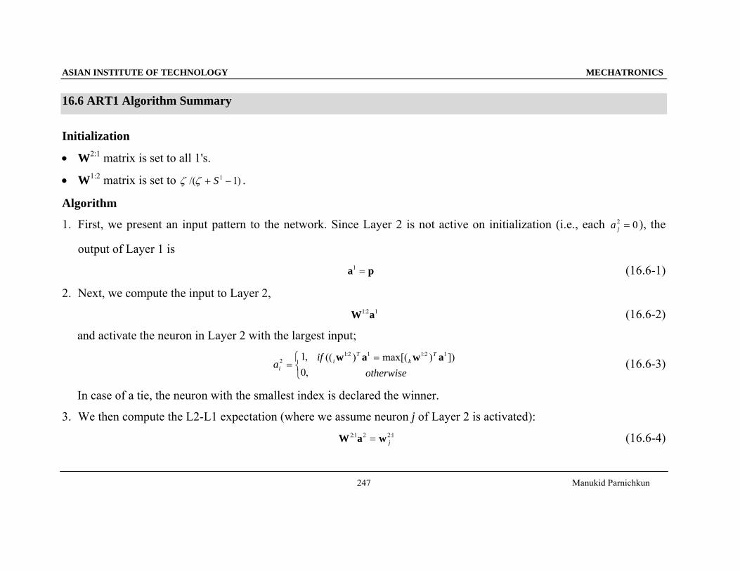
16.6 ART1 Algorithm Summary

Initialization

• W2:1 matrix is set to all 1's.

• W1:2 matrix is set to )1/( 1 −+ Sζζ .

Algorithm

1. First, we present an input pattern to the network. Since Layer 2 is not active on initialization (i.e., each 02 =ja ), the

output of Layer 1 is

pa =1 (16.6-1)

2. Next, we compute the input to Layer 2, 12:1 aW (16.6-2)

and activate the neuron in Layer 2 with the largest input;

⎩⎨⎧

=,0,12

ia otherwise

if Tk

Ti ]))max[()(( 12:112:1 awaw = (16.6-3)

In case of a tie, the neuron with the smallest index is declared the winner.

3. We then compute the L2-L1 expectation (where we assume neuron j of Layer 2 is activated): 1:221:2

jwaW = (16.6-4)


Manukid Parnichkun

248

4. Now that Layer 2 is active, we adjust the Layer 1 output to include the L2-Ll expectation:

pwpa =∩= 1:21j (16.6-5)

5. Next, the Orienting Subsystem determines the degree of match between the expectation and the input pattern:

⎩⎨⎧

=,0,10a

otherwiseif ]/[ 221 ρ<pa (16.6-6)

6. If a0= 1, then we set 02 =ja , inhibit it until an adequate match occurs (resonance), and return to step 1. If a0= 0, we

continue with step 7.

7. Resonance has occurred. Therefore we update row j of W1:2:

121

121

−+=

a

awζ

ζ:j (16.6-7)

8. We now update column j of W2:1: 11:2 aw =j (16.6-8)

9. We remove the input pattern, restore all inhibited neurons in Layer 2, and return to step 1 with a new input pattern.

• The input patterns continue to be applied to the network until the weights stabilize (do not change).

• ART1 algorithm always forms stable clusters for any set of input patterns.


Manukid Parnichkun

249

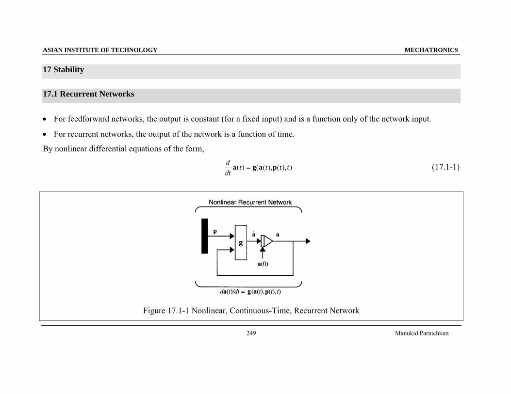
17 Stability

17.1 Recurrent Networks

• For feedforward networks, the output is constant (for a fixed input) and is a function only of the network input.

• For recurrent networks, the output of the network is a function of time.

By nonlinear differential equations of the form, ddt

t t t ta g a p( ) ( ( ), ( ), )= (17.1-1)

Figure 17.1-1 Nonlinear, Continuous-Time, Recurrent Network


Manukid Parnichkun

250

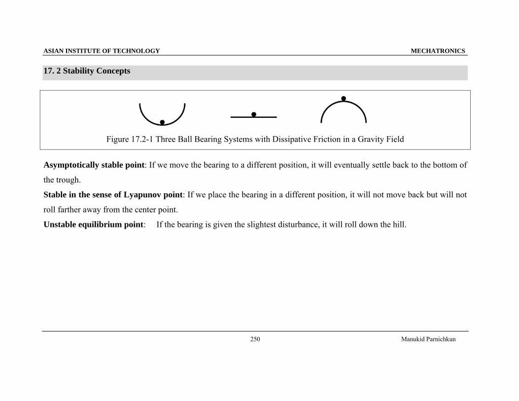
17. 2 Stability Concepts

Figure 17.2-1 Three Ball Bearing Systems with Dissipative Friction in a Gravity Field

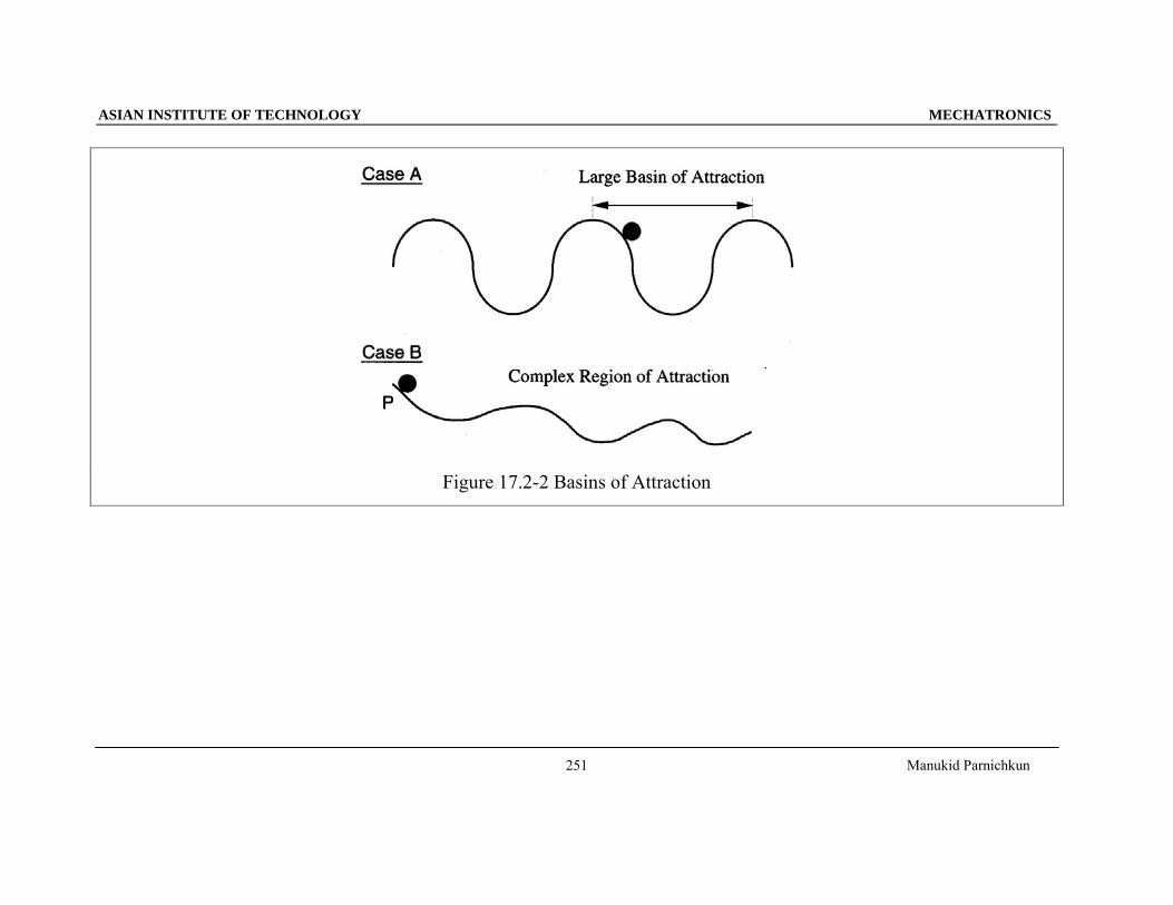
Asymptotically stable point: If we move the bearing to a different position, it will eventually settle back to the bottom of

the trough.

Stable in the sense of Lyapunov point: If we place the bearing in a different position, it will not move back but will not

roll farther away from the center point.

Unstable equilibrium point: If the bearing is given the slightest disturbance, it will roll down the hill.


Manukid Parnichkun

251

Figure 17.2-2 Basins of Attraction


Manukid Parnichkun

252

17.2.1 Definitions

An equilibrium point; a point a* where the derivative is zero.

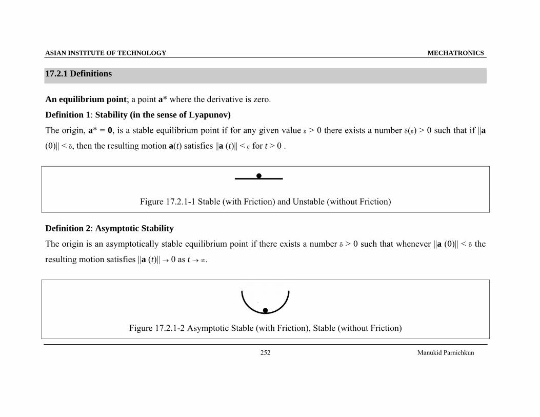
Definition 1: Stability (in the sense of Lyapunov)

The origin, a* = 0, is a stable equilibrium point if for any given value ε > 0 there exists a number δ(ε) > 0 such that if ||a

(0)|| < δ, then the resulting motion a(t) satisfies ||a (t)|| < ε for t > 0 .

Figure 17.2.1-1 Stable (with Friction) and Unstable (without Friction)

Definition 2: Asymptotic Stability

The origin is an asymptotically stable equilibrium point if there exists a number δ > 0 such that whenever ||a (0)|| < δ the

resulting motion satisfies ||a (t)|| → 0 as t → ∞.

Figure 17.2.1-2 Asymptotic Stable (with Friction), Stable (without Friction)


Manukid Parnichkun

253

Definition 3: Positive Definite

A scalar function V(a) is positive definite if V(0) = 0 and V(a) > 0 for a ≠ 0.

Definition 4: Positive Semidefinite

A scalar function V(a) is positive semidefinite if V(a) ≥ 0 for all a.

17.3 Lyapunov Stability Theorem

Consider the autonomous (unforced, no explicit time dependence) system,

ddta g a= ( ) (17.3-1)

Theorem 1: Lyapunov Stability Theorem

If a positive definite function V(a) can be found such that dV(a)/dt is negative semidefinite, then the origin (a = 0) is

stable for the system of (17.3-1). If a positive definite function V(a) can be found such that dV(a)/dt is negative definite,

then the origin (a = 0) is asymptotically stable. In each case, V is called a Lyapunov function of the system.


Manukid Parnichkun

254

17.4 Pendulum Example

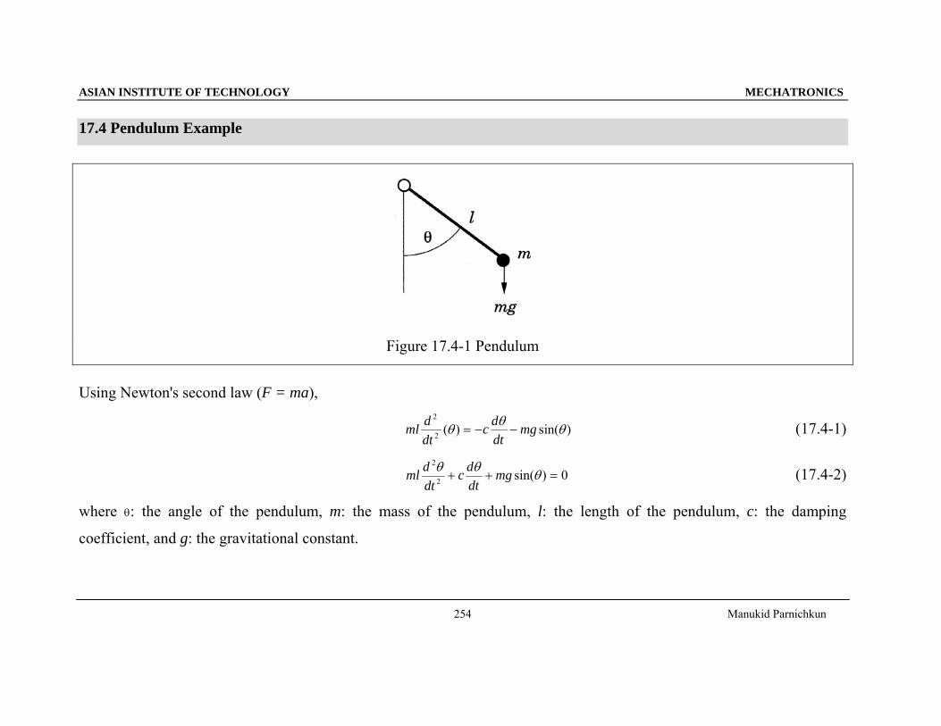
Figure 17.4-1 Pendulum

Using Newton's second law (F = ma),

ml ddt

c ddt

mg2

2 ( ) sin( )θ θ θ= − − (17.4-1)

ml ddt

c ddt

mg2

2 0θ θ θ+ + =sin( ) (17.4-2)

where θ: the angle of the pendulum, m: the mass of the pendulum, l: the length of the pendulum, c: the damping

coefficient, and g: the gravitational constant.


Manukid Parnichkun

255

State variables,

a1 = θ and a ddt2 =θ (17.4-3)

dadt

a12= (17.4-4)

dadt

gl

a cml

a21 2= − −sin( ) (17.4-5)

Consider the stability of the origin (a = 0), dadt

a12 0= = (17.4-6)

dadt

gl

a cml

a gl

cml

21 2 0 0 0= − − = − − =sin( ) sin( ) ( ) (17.4-7)

• The origin is an equilibrium point.

Total (kinetic and potential) energy of the pendulum

V ml a mgl a( ) ( ) ( cos( ))a = + −12

122

21 (17.4-8)

ddt

V V g Va

dadt

Va

dadt

T( ) [ ( )] ( )a a a= ∇ = ⎛⎝⎜

⎞⎠⎟+ ⎛

⎝⎜⎞⎠⎟

∂∂

∂∂1

1

2

2 (17.4-9)

ddt

V mgl a a ml a gl

a cml

a cl a( ) ( sin( )) ( ) sin( ) ( )a = + − −⎛⎝⎜

⎞⎠⎟= − ≤1 2

22 1 2 2

2 0 (17.4-10)


Manukid Parnichkun

256

• dV(a)/dt is negative semidefinite.

• From Lyapunov's theorem, then, we know that the origin is a stable point.

• However, we cannot say, from the theorem and this Lyapunov function, that the origin is asymptotically stable.

• As long as the pendulum has friction, it will eventually settle in a vertical position, the origin is asymptotically stable.

When g = 9.8, m = 1, 1 = 9.8, c = 1.96, dadt

a12= (17.4-11)

dadt

a a21 20 2= − −sin( ) . (17.4-12)

V a a= + −⎡⎣⎢

⎤⎦⎥

( . ) ( ) ( cos( ))9 8 12

122

21 (17.4-13)

dVdt

a= −( . )( )19 208 22 (17.4-14)


Manukid Parnichkun

257

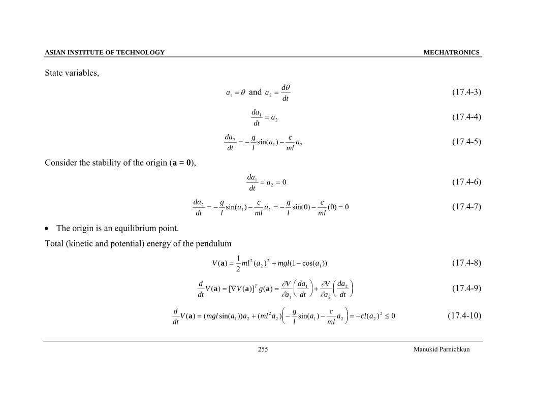
Figure 17.4-2 Pendulum Energy Surface, Three Possible Minimum Points of the Energy Surface at 0 and ±2π

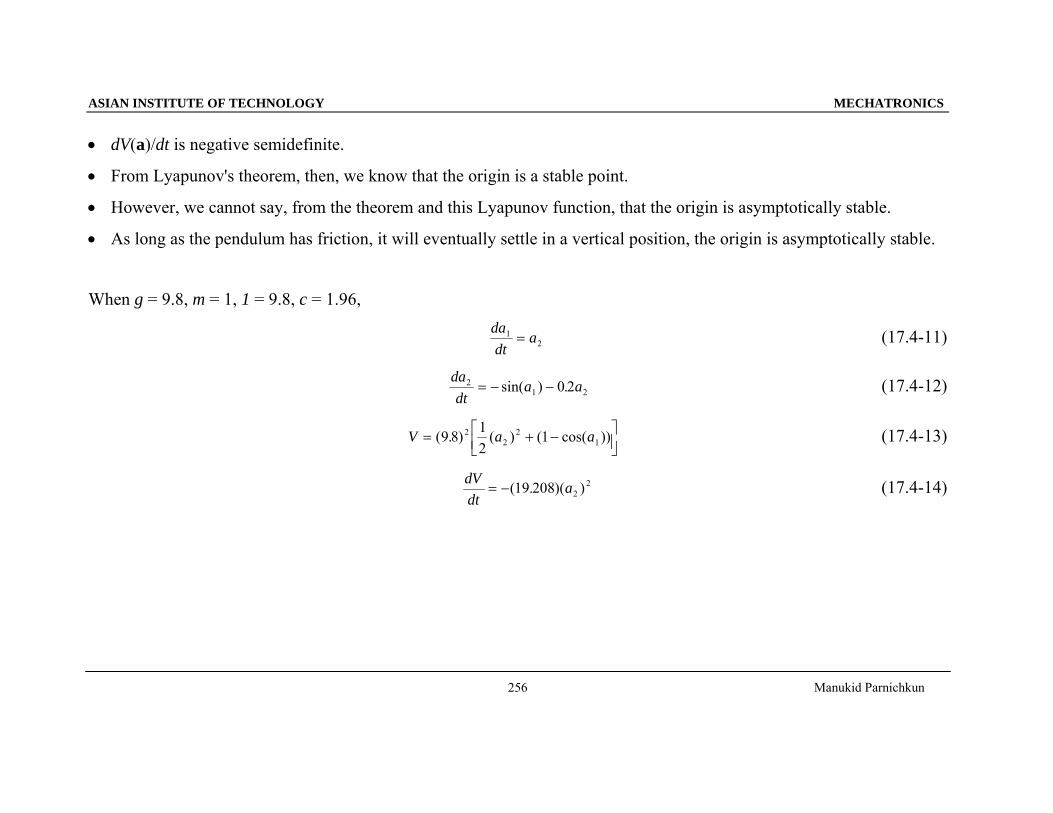
Figure 17.4-3 Pendulum Response on State Variable Plane, a1(0) = 1.3 radians (74°), a2(0) = 1.3 radians per second


Manukid Parnichkun

258

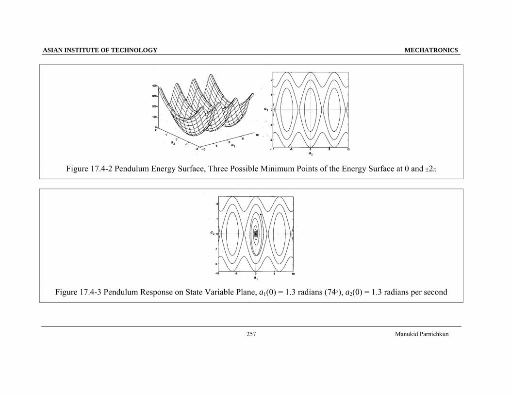
Figure 17.4-4 State Variables vs. Time

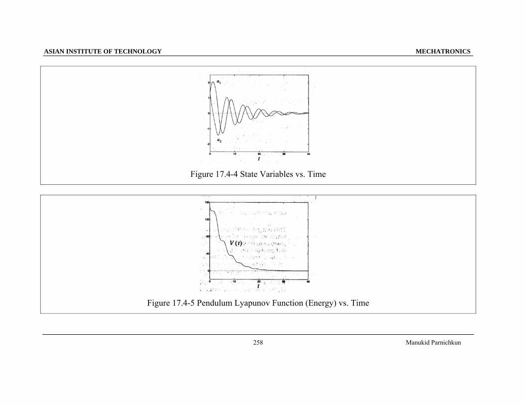
Figure 17.4-5 Pendulum Lyapunov Function (Energy) vs. Time


Manukid Parnichkun

259

17.5 Lasalle's Invariance Theorem

Definition 5: Lyapunov Function

Let V be a continuously differentiable function from Rn to R. If G is any subset of Rn, we say that V is a Lyapunov

function on G for the system da/dt = g(a) if

)())(()( agaa TVdt

dV∇= (17.5-1)

does not change sign on G.

Definition 6: Set Z

}_____,0/)(:{ GofclosuretheindtdVZ aaa == (17.5-2)

Definition 7: Invariant Set

A set of points in Rn is invariant with respect to da/dt = g(a) if every solution of da/dt = g(a) starting in that set remains in

the set for all time.

Definition 8: Set L

L is defined as the largest invariant set in Z.

• If L has only one stable point, then that point is asymptotically stable.


Manukid Parnichkun

260

Theorem 2: Lasalle's Invariance Theorem

If V is a Lyapunov function on G for da/dt = g(a), then each solution a(t) that remains in G for all t > 0 approaches

L° = L ∩G as t → ∞. (G is a basin of attraction for L, which has all of the stable points.) If all trajectories are bounded,

then a(t) → L as t → ∞.

• If a trajectory stays in G, then it will either converge to L, or it will go to infinity. If all trajectories are bounded, then

all trajectories will converge to L.

Corollary 1: Lasalle's Corollary

Let G be a component (one connected subset) of

})(:{ ηη <=Ω aa V (17.5-3)

• Assume that G is bounded, dV(a)/dt ≤ 0 on the set G, and let the set L° = closure(L ∩ G) be a subset of G. Then L° is

an attractor, and G is in its region of attraction.


Manukid Parnichkun

261

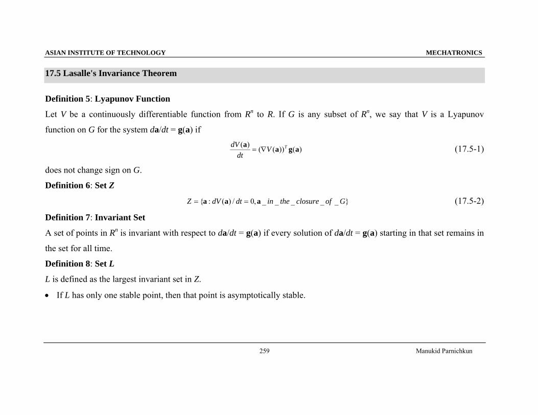
17.5.1 Example

η = 100,

}100)(:{100 ≤=Ω aa V (17.5.1-1)

Figure 17.5.1-1 Illustration of the Set Ω100


Manukid Parnichkun

262

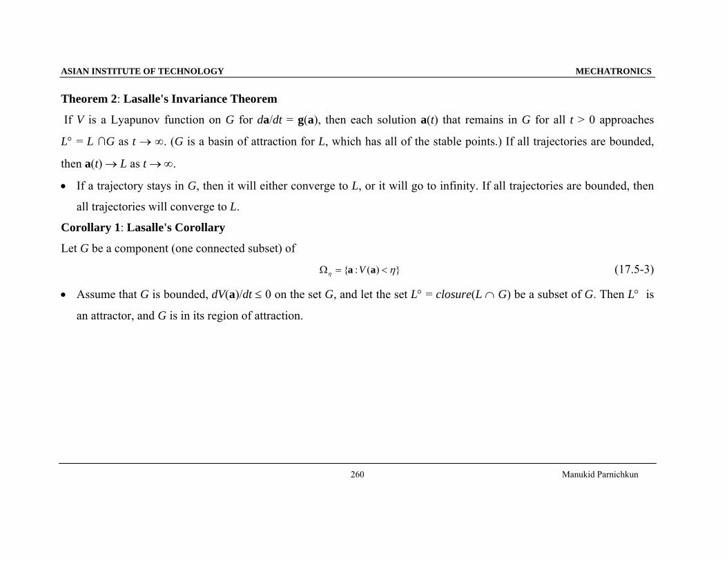
By choosing the component of Ω100 that contains a = 0.

Figure 17.5.1-2 Illustration of the Set G

}_____,0:{}_____,0/)(:{ 2 GofclosuretheinaGofclosuretheindtdVZ aaaaa ==== (17.5.1-2)

}6.16.1,0:{ 12 ≤≤−== aaZ a (17.5.1-3)


Manukid Parnichkun

263

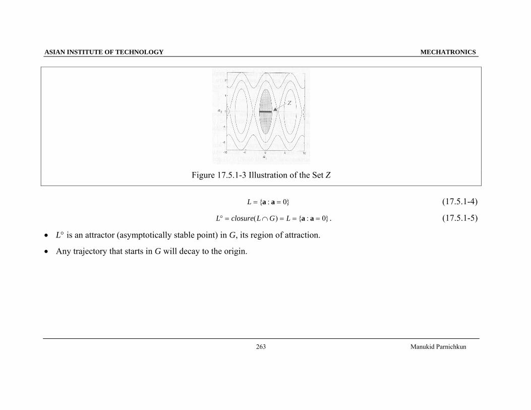
Figure 17.5.1-3 Illustration of the Set Z

}0:{ == aaL (17.5.1-4)

}0:{)( ===∩=° aaLGLclosureL . (17.5.1-5)

• L° is an attractor (asymptotically stable point) in G, its region of attraction.

• Any trajectory that starts in G will decay to the origin.


Manukid Parnichkun

264

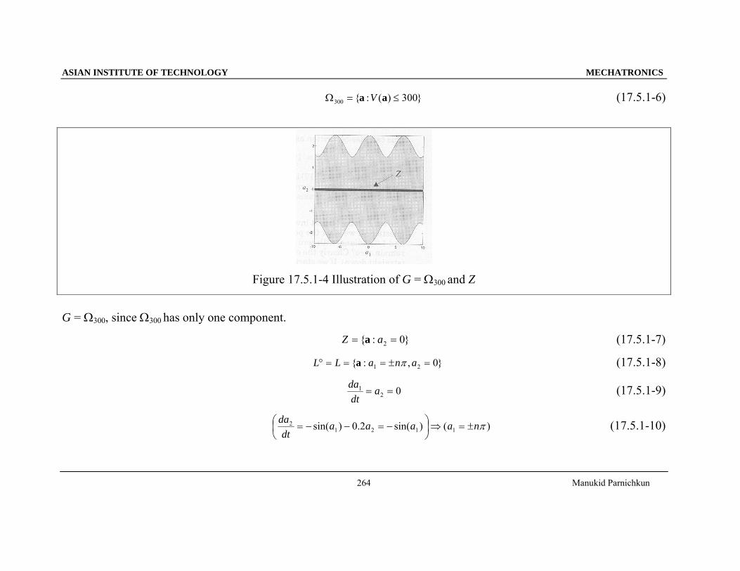
}300)(:{300 ≤=Ω aa V (17.5.1-6)

Figure 17.5.1-4 Illustration of G = Ω300 and Z

G = Ω300, since Ω300 has only one component.

}0:{ 2 == aZ a (17.5.1-7)

}0,:{ 21 =±===° anaLL πa (17.5.1-8)

021 == a

dtda (17.5.1-9)

)()sin(2.0)sin( 11212 πnaaaa

dtda

±=⇒⎟⎠⎞

⎜⎝⎛ −=−−= (17.5.1-10)


Manukid Parnichkun

265

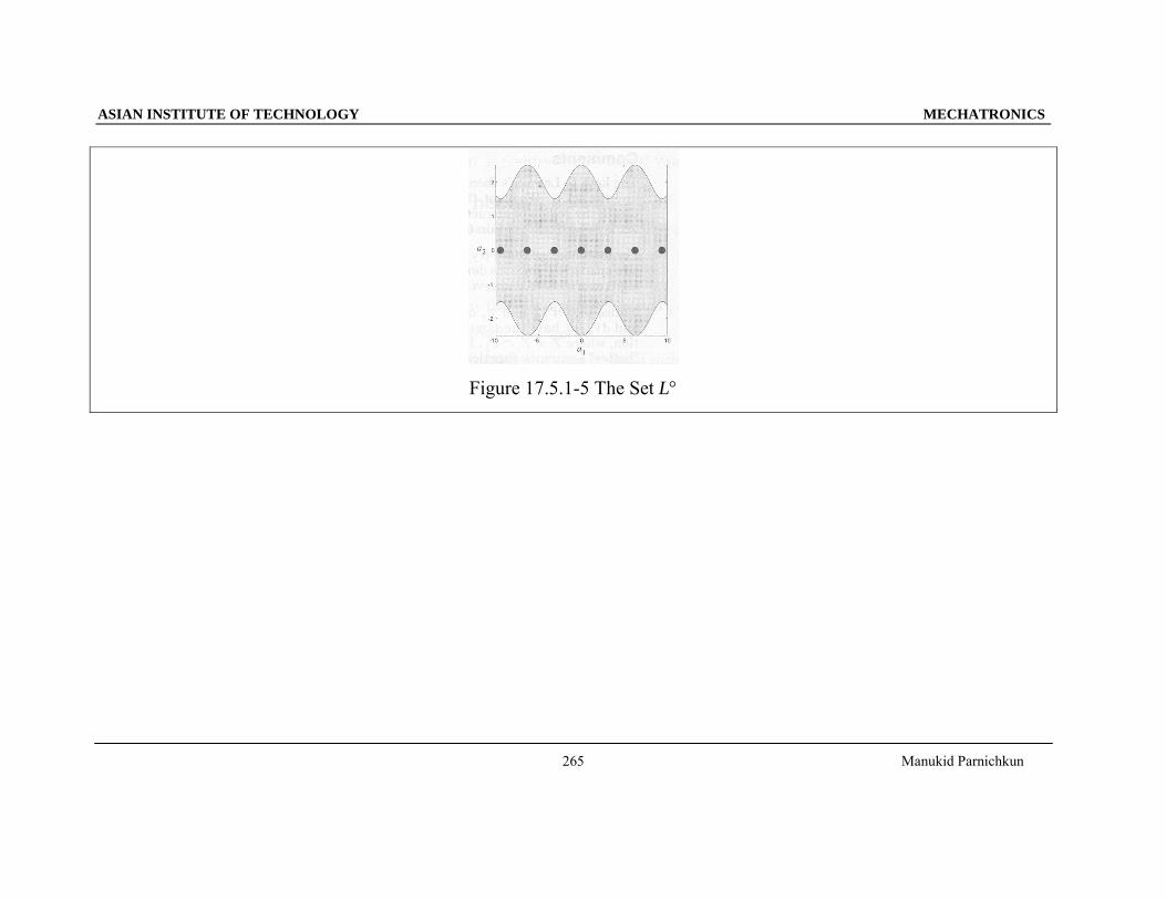
Figure 17.5.1-5 The Set L°


Manukid Parnichkun

266

18 Hopfield Network

18.1 Hopfield Model

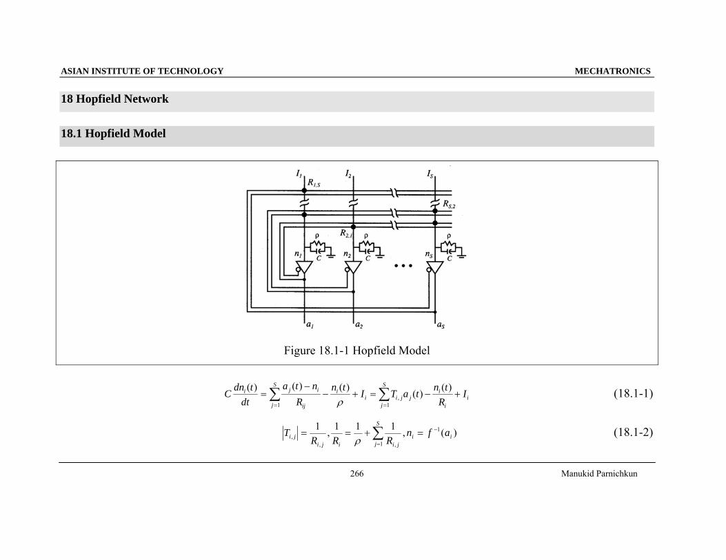
Figure 18.1-1 Hopfield Model

ii

iS

jjjii

iS

j ij

iji IR

tntaTItnR

ntadt

tdnC +−=+−−

= ∑∑==

)()()()()(1

,1 ρ

(18.1-1)

∑=

−=+==S

jii

jiijiji afn

RRRT

1

1

,,, )(,111,1

ρ (18.1-2)


Manukid Parnichkun

267

By multiplying with Ri, iii

S

jjjii

ii IRtntaTR

dttdnCR +−= ∑

=

)()()(1

, (18.1-3)

Defining, iiijiijii IRbTRwCR === ,, ,,ε (18.1-4)

i

S

jjjii

i btawtndt

tdn++−= ∑

=1, )()()(ε (18.1-5)

bWann++−= )()()( tt

dttdε (18.1-6)

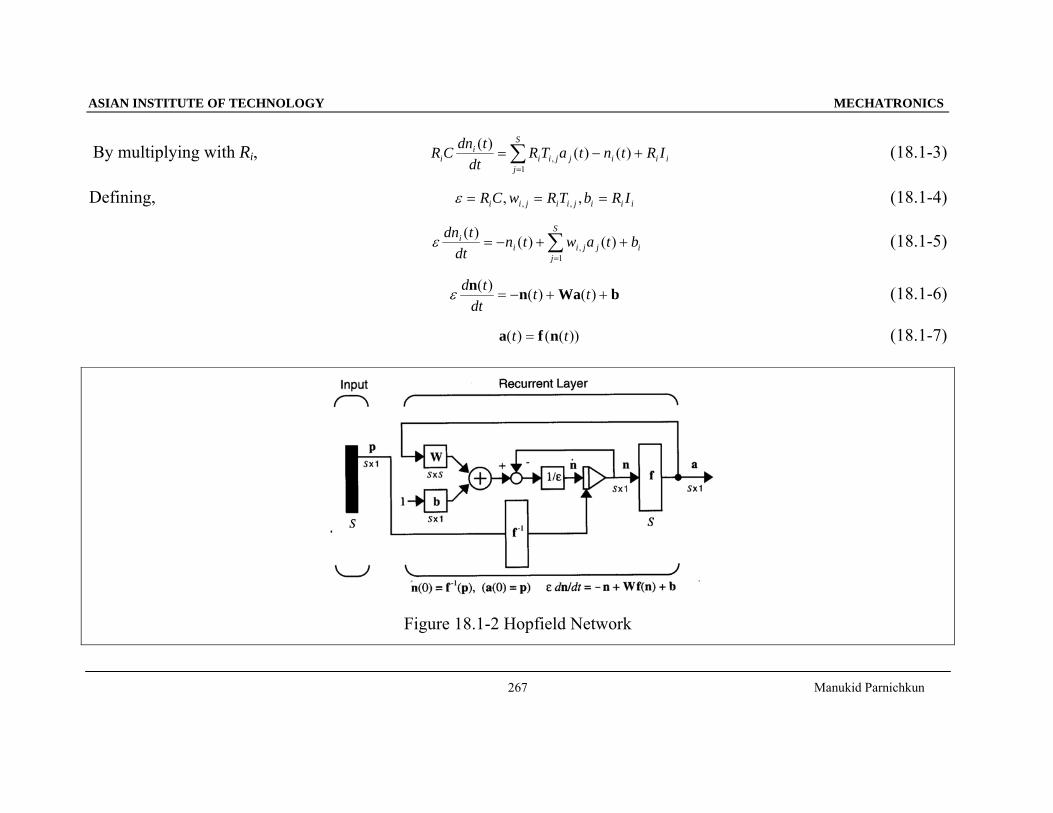
))(()( tt nfa = (18.1-7)

Figure 18.1-2 Hopfield Network


Manukid Parnichkun

268

18.2 Lyapunov Function

Lyapunov function in Lasalle’s theorem of Hopfield network,

∑ ∫=

− −⎪⎭

⎪⎬⎫

⎪⎩

⎪⎨⎧

+−=S

i

Ta

Ti

duufV1 0

1 )(21)( abWaaa (18.2-1)

dtd

dtd

dtd

dtd TTTTT aWaaWaaWaaWaa −=−=∇−=− ][][

21}

21{ (18.2-2)

dtdan

dtdaaf

dtdaduuf

dadduuf

dtd i

ii

ii

a

i

a ii

==⎪⎭

⎪⎬⎫

⎪⎩

⎪⎨⎧

=⎪⎭

⎪⎬⎫

⎪⎩

⎪⎨⎧

−−− ∫∫ )()()( 1

0

1

0

1 (18.2-3)

dtdduuf

dtd T

S

i

ai an=⎥⎥⎦

⎤

⎢⎢⎣

⎡

⎪⎭

⎪⎬⎫

⎪⎩

⎪⎨⎧

∑ ∫=

−

1 0

1 )( (18.2-4)

dtd

dtd

dtd TTTT abaabab −=−∇=− ][}{ (18.2-5)

dtd

dtd

dtd

dtdV

dtd TTTTTT abnWaabanaWaa ][)( −+−=−+−= (18.2-6)

TTTT

dttd⎥⎦⎤

⎢⎣⎡−=−+−

)(][ nbnWa ε (18.2-7)

∑=

⎟⎠⎞

⎜⎝⎛⎟⎠⎞

⎜⎝⎛−=⎥⎦

⎤⎢⎣⎡−=

S

i

iiT

dtda

dtdn

dtd

dttdV

dtd

1

)()( εε ana (18.2-8)


Manukid Parnichkun

269

dtdaaf

dadaf

dtd

dtdn i

ii

ii )]([)]([ 11 −− == (18.2-9)

∑∑=

−

=⎟⎠⎞

⎜⎝⎛⎟⎟⎠

⎞⎜⎜⎝

⎛−=⎟

⎠⎞

⎜⎝⎛⎟⎠⎞

⎜⎝⎛−=

S

i

ii

i

S

i

ii

dtdaaf

dad

dtda

dtdnV

dtd

1

21

1

)]([)( εεa (18.2-10)

If f-1(ai) is an increasing function,

0)]([ 1 >−i

i

afdad (18.2-11)

0)( ≤aVdtd (18.2-12)

• If f-1(ai) is an increasing function, dV(a)/dt is a negative semidefinite function. V(a) is a valid Lyapunov function.

18.2.1 Invariant Sets

SRG ⊂ (18.2.1-1)

}_____,0/)(:{ GofclosuretheindtdVZ aaa == (18.2.1-2)

}:{ 0aa ==dtdZ , which is set of equilibrium points (18.2.1-2)

ZL = (18.2.1-3)

• All points in Z are potential attractors.


Manukid Parnichkun

270

18.2.2 Example

⎟⎠⎞

⎜⎝⎛== −

2tan2)( 1 nnfa γπ

π (18.2.2-1)

1,1,0 211,22,1212,21,1 ======== CCRRRR ρρ (18.2.2-2)

⎥⎦

⎤⎢⎣

⎡=

0110

W (18.2.2-3)

1== CRiε (18.2.2-4)

With γ = 1.4 and I1 = I2 = 0,

⎥⎦

⎤⎢⎣

⎡=

00

b (18.2.2-5)

The Lyapunov function,

∑ ∫=

− −⎪⎭

⎪⎬⎫

⎪⎩

⎪⎨⎧

+−=S

i

Ta

Ti

duufV1 0

1 )(21)( abWaaa (18.2.2-6)

[ ] 212

121 01

1021

21 aa

aa

aaT −=⎥⎦

⎤⎢⎣

⎡⎥⎦

⎤⎢⎣

⎡−=− Waa (18.2.2-7)

iiiaaa

uduuduuf000

1 22

coslog22

tan2)( ⎥⎦

⎤⎢⎣

⎡⎥⎦

⎤⎢⎣

⎡⎟⎠⎞

⎜⎝⎛−=⎟

⎠⎞

⎜⎝⎛= ∫∫ −

ππ

γππ

γπ (18.2.2-8)


Manukid Parnichkun

271

⎥⎦

⎤⎢⎣

⎡⎟⎠⎞

⎜⎝⎛−=∫ −

i

a

aduufi

2coslog4)( 2

0

1 πγπ

(18.2.2-9)

⎥⎦⎤

⎢⎣⎡ +−−= }

2log{cos}

2log{cos

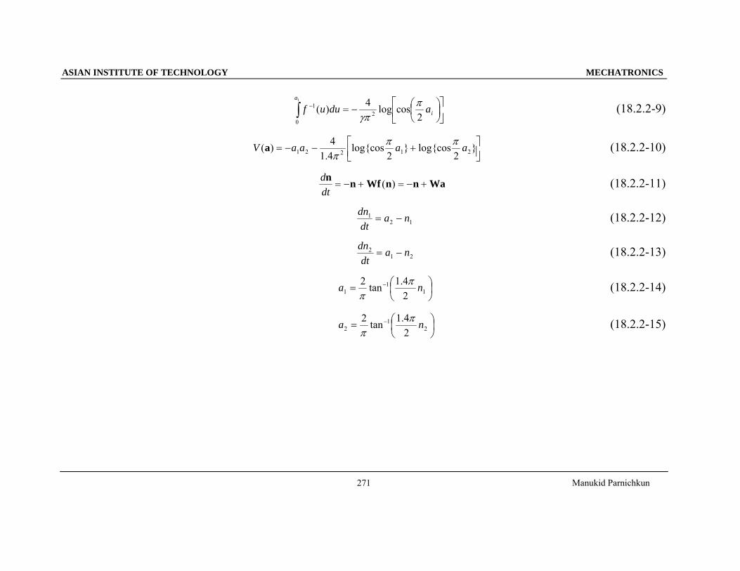
4.14)( 21221 aaaaV πππ

a (18.2.2-10)

WannWfnn+−=+−= )(

dtd (18.2.2-11)

121 na

dtdn

−= (18.2.2-12)

212 na

dtdn

−= (18.2.2-13)

⎟⎠⎞

⎜⎝⎛= −

11

1 24.1tan2 na π

π (18.2.2-14)

⎟⎠⎞

⎜⎝⎛= −

21

2 24.1tan2 na π

π (18.2.2-15)


Manukid Parnichkun

272

Figure 18.2.2-1 Hopfield Example Lyapunov Function and Trajectory

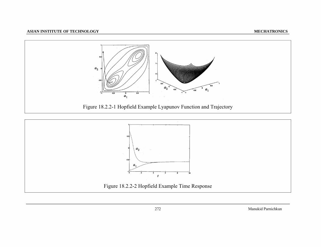
Figure 18.2.2-2 Hopfield Example Time Response


Manukid Parnichkun

273

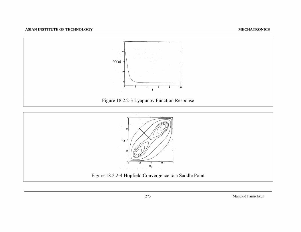
Figure 18.2.2-3 Lyapunov Function Response

Figure 18.2.2-4 Hopfield Convergence to a Saddle Point


Manukid Parnichkun

274

18.2.3 Hopfield Attractors

The potential attractors of the Hopfield network are equilibrium points.

0a=

dtd (18.2.3-1)

The minima of a function must be stationary points. The stationary points of V(a),

0=⎥⎦

⎤⎢⎣

⎡∂∂

∂∂

∂∂

=∇Sa

VaV

aVV L

21

(18.2.3-2)

∑ ∫=

− −⎪⎭

⎪⎬⎫

⎪⎩

⎪⎨⎧

+−=S

i

Ta

Ti

duufV1 0

1 )(21)( abWaaa (18.2.3-3)

⎥⎦⎤

⎢⎣⎡−=−+−=∇

dttdV )(][)( nbnWaa ε (18.2.3-4)

dtdaaf

dadaf

dtd

dtdnV

ai

ii

ii

i

)]([)])(([)( 11 −− −=−=−=∂∂ εεεa (18.2.3-5)

If f--1(a) is linear,

)(aa Vdtd

∇−= α (18.2.3-6)

• The response of the Hopfield network is steepest descent.

• If you are in a region where f--1(a) is approximately linear, the network solution approximates steepest descent.


Manukid Parnichkun

275

For an increasing function,

0)]([ 1 >−iaf

dtd (18.2.3-7)

The points for which

0a=

dttd )( (18.2.3-8)

are also the points where

0a =∇ )(V (18.2.3-9)

• The attractors, which are members of the set L, will also be stationary points of the Lyapunov function V(a) .


Manukid Parnichkun

276

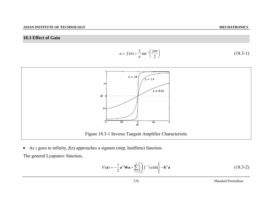
18.3 Effect of Gain

a f n n= = ⎛

⎝⎜⎞⎠⎟

−( ) tan22

1

πγπ (18.3-1)

Figure 18.3-1 Inverse Tangent Amplifier Characteristic

• As γ goes to infinity, f(n) approaches a signum (step, hardlims) function.

The general Lyapunov function,

V f u duTa

i

ST

i

( ) ( )a a Wa b a= − +⎧⎨⎪

⎩⎪

⎫⎬⎪

⎭⎪−−

=∫∑1

21

01

(18.3-2)


Manukid Parnichkun

277

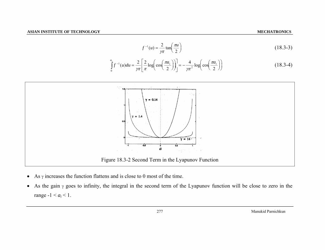
f u u− = ⎛⎝⎜

⎞⎠⎟

1 22

( ) tanγπ

π (18.3-3)

f u du a aai i

i−∫ = ⎛

⎝⎜⎞⎠⎟

⎛⎝⎜

⎞⎠⎟

⎡

⎣⎢

⎤

⎦⎥ = − ⎛

⎝⎜⎞⎠⎟

⎛⎝⎜

⎞⎠⎟1

02

2 22

42

( ) log cos log cosγπ π

πγπ

π (18.3-4)

Figure 18.3-2 Second Term in the Lyapunov Function

• As γ increases the function flattens and is close to 0 most of the time.

• As the gain γ goes to infinity, the integral in the second term of the Lyapunov function will be close to zero in the

range -1 < ai < 1.


Manukid Parnichkun

278

The high-gain Lyapunov function,

V T T( )a a Wa b a= − −12

(18.3-5)

V cT T T T( )a a Wa b a a Aa d a= − − = + +12

12

(18.3-6)

∇ = = − = − =2 0V c( ) , ,a A W d b (18.3-7)

∇ = − =−

−⎡

⎣⎢

⎤

⎦⎥

2 0 11 0

V ( )a W (18.3-8)

∇ − =− −− −

= − = + −2 211

1 1 1V I( ) ( )( )a λλ

λλ λ λ (18.3-9)

The eigenvalues are λ1 = -l and λ2 = l. The eigenvectors are

z z1 2

11

11

=⎡

⎣⎢⎤

⎦⎥ =

−⎡

⎣⎢

⎤

⎦⎥, (18.3-10)

There will be constrained minima at the two corners of the hypercube

a =⎡

⎣⎢⎤

⎦⎥

11

and a =−−⎡

⎣⎢

⎤

⎦⎥

11

(18.3-11)


Manukid Parnichkun

279

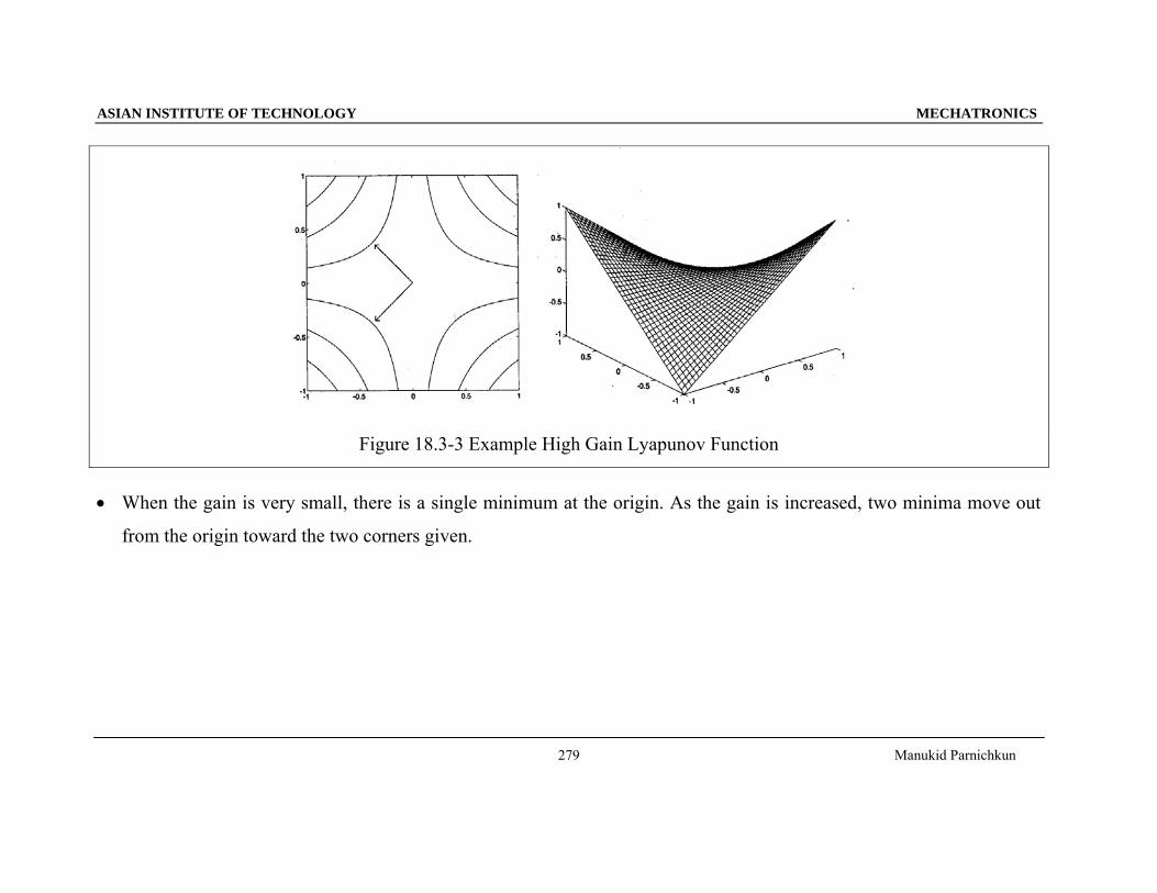
Figure 18.3-3 Example High Gain Lyapunov Function

• When the gain is very small, there is a single minimum at the origin. As the gain is increased, two minima move out

from the origin toward the two corners given.


Manukid Parnichkun

280

18.4 Hopfield Design

• The Hopfield network does not have a learning law associated with it. It is not trained, nor does it learn on its own.

• A design procedure based on the Lyapunov function is used to determine the weight matrix.


V T T( )a a Wa b a= − −12

(18.4-1)

• The Hopfield design technique is to choose the weight matrix W and the bias vector b so that V takes on the form of a

function to be minimized.

18.4.1 Content-Addressable Memory

• When an input pattern is presented to the network, the network should produce the stored pattern that most closely

resembles the input pattern.

• The initial network output is assigned to the input pattern. The network output should then converge to the prototype

pattern closest to the input pattern.

The prototype patterns,

{ , , }p p p1 2 K Q (18.4.1-1)


Manukid Parnichkun

281

• Each of these vectors consists of S elements, having the values 1 or -1.

• Q << S.

Quadratic performance index,

J qT

q

Q

( ) ([ ] )a p a= −=∑1

22

1

(18.4.1-2)

• If the elements of the vectors a are restricted to be ±1, this function is minimized at the prototype patterns.

When the prototype patterns are orthogonal, the performance index at one of the prototype patterns,

J p p p p p( ) ([ ] ) ([ ] )j qT

jq

Q

jT

jS

= − = − = −=∑1

212 2

2

1

22

(18.4.1-3)

• J(a) will be largest (least negative) when a is not close to any prototype pattern, and will be smallest (most negative)

when a is equal to any one of the prototype patterns.

When the weight matrix applies the supervised Hebb rule (with target patterns being the same as input patterns) as

W p p==∑ q q

T

q

Q

( )1

(18.4.1-4)

b 0= (18.4.1-5)

The Lyapunov function,

V T Tq q

T

q

QT

q qT

q

Q

( ) ( ) ( )a a Wa a p p a a p p a= − = −⎡

⎣⎢

⎤

⎦⎥ = −

= =∑ ∑1

212

121 1

(18.4.1-6)


Manukid Parnichkun

282

V JqT

q

Q

( ) ([ ] ) ( )a p a a= − ==∑1

22

1

(18.4.1-7)

• The Lyapunov function is indeed equal to the quadratic performance index for the content-addressable memory

problem.

• The Hopfield network output will tend to converge to the stored prototype patterns.

• If there is significant correlation between the prototype patterns, the supervised Hebb rule does not work well. In that

case the pseudoinverse technique has been suggested.

• In the best situation, where the prototype patterns are orthogonal, every prototype pattern will be an equilibrium point

of the network. However, there will be many other equilibrium points as well. The network may well converge to a

pattern that is not one of the prototype patterns.

• A general rule is that, when using the Hebb rule, the number of stored patterns can be no more than 15% of the number

of neurons.


Manukid Parnichkun

283

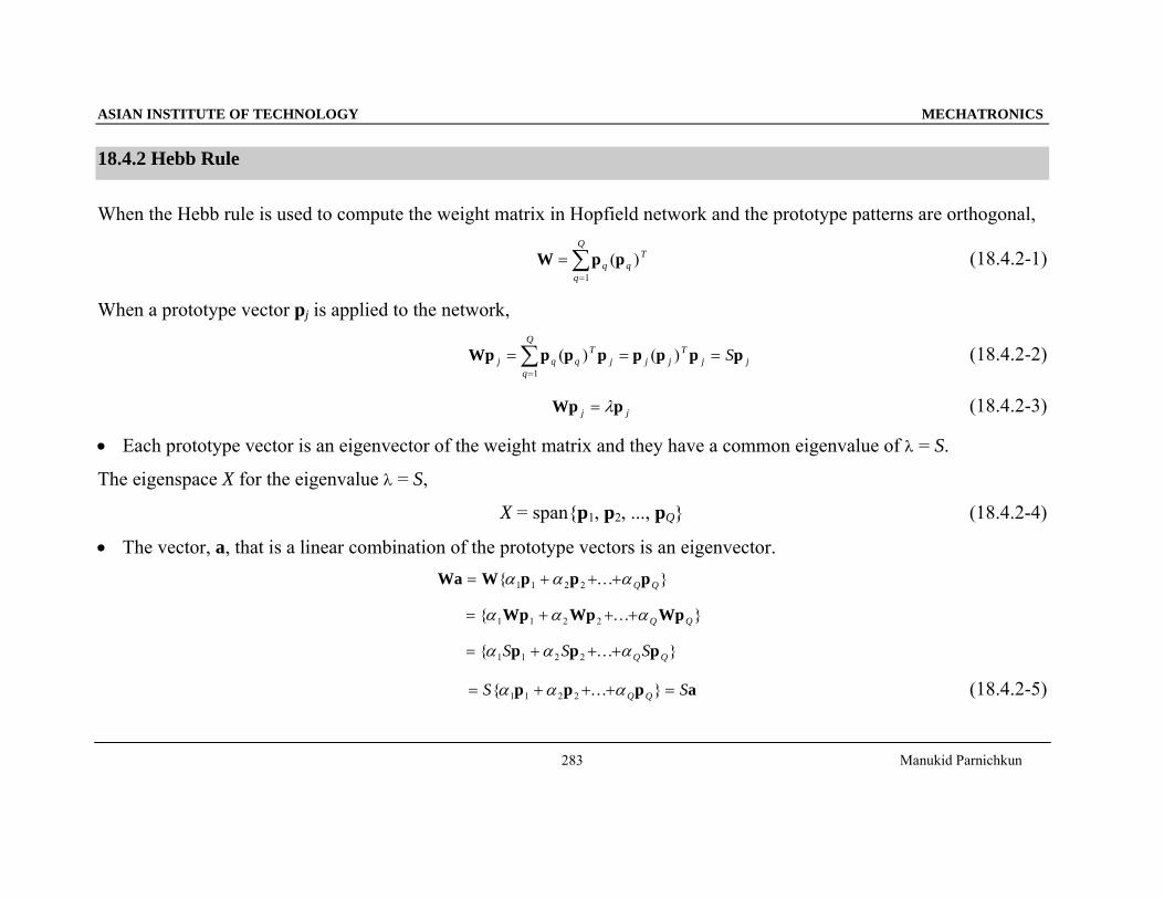
18.4.2 Hebb Rule

When the Hebb rule is used to compute the weight matrix in Hopfield network and the prototype patterns are orthogonal,

W p p==∑ q q

T

q

Q

( )1

(18.4.2-1)

When a prototype vector pj is applied to the network,

Wp p p p p p p pj q qT

jq

Q

j jT

j jS= = ==∑ ( ) ( )

1

(18.4.2-2)

Wp pj j= λ (18.4.2-3)

• Each prototype vector is an eigenvector of the weight matrix and they have a common eigenvalue of λ = S.

The eigenspace X for the eigenvalue λ = S,

X = span{p1, p2, ..., pQ} (18.4.2-4)

• The vector, a, that is a linear combination of the prototype vectors is an eigenvector.

Wa W p p p= + + +{ }α α α1 1 2 2 K Q Q

= + + +{ }α α α1 1 2 2Wp Wp WpK Q Q

= + + +{ }α α α1 1 2 2S S SQ Qp p pK

= + + + =S SQ Q{ }α α α1 1 2 2p p p aK (18.4.2-5)


Manukid Parnichkun

284

The entire space RS can be divided into two disjoint sets,

R X XS = ∪ ⊥ (18.4.2-6)

where X ⊥ : the orthogonal complement of X.

• Every vector in X ⊥ is orthogonal to every vector in X.

a ∈ X ⊥ ,

( ) , , , ,p aqT q Q= =0 1 2 K (18.4.2-7)

Wa p p a p 0 a= = ⋅ = = ⋅==∑∑ q q

Tq

q

Q

q

Q

( ) ( )0 011

(18.4.2-8)

• X ⊥ defines an eigenspace for the repeated eigenvalue λ = 0.

Summary

• The weight matrix has two eigenvalues, S and 0.

• The eigenspace for the eigenvalue S is the space spanned by the prototype vectors.

• The eigenspace for the eigenvalue 0 is the orthogonal complement of the space spanned by the prototype vectors.

Hessian matrix for the high-gain Lyapunov function V,

∇ = −2V W (18.4.2-9)

• The eigenvalues for ∇2V will be -S and 0.


Manukid Parnichkun

285

• The high-gain Lyapunov function is a quadratic function.

• The first eigenvalue is negative, V will have negative curvature in X.

• The second eigenvalue is zero, V will have zero curvature in X ⊥ .

• Because V has negative curvature in X, the trajectories of the Hopfield network will tend to fall into the corners of the

hypercube {a:-1<ai< 1} that are contained in X.

• By using the Hebb rule, there will be at least two minima of the Lyapunov function for each prototype vector.

• If pq is a prototype vector, then -pq will also be in the space spanned by the prototype vectors, X.

• The negative of each prototype vector will be one of the comers of the hypercube {a:-1<ai< 1} that are contained in X.

There will also be a number of other minima of the Lyapunov function that do not correspond to prototype patterns.

• The minima of V are in the corners of the hypercube {a:-1<ai< 1} that are contained in X.

• These corners will include the prototype patterns, and also some linear combinations of the prototype patterns.

• The minima that are not prototype patterns are often referred to as spurious patterns.


Manukid Parnichkun

286

Example:

When 1,1,0 211,22,1212,21,1 ======== CCRRRR ρρ ,

⎥⎦

⎤⎢⎣

⎡=′

0110

W (18.4.2-10)

An attractor by using high gain Lyapunov function,

p1

11

=⎡

⎣⎢⎤

⎦⎥ (18.4.2-11)

By using the Hebb rule with one prototype pattern at the attractor,

[ ]W p p= =⎡

⎣⎢⎤

⎦⎥ =

⎡

⎣⎢

⎤

⎦⎥1 1

11

1 11 11 1

( )T (18.4.2-12)

⎥⎦

⎤⎢⎣

⎡=−=′

0110

IWW (18.4.2-13)


V T T( )a a Wa a a= − = −⎡

⎣⎢

⎤

⎦⎥

12

12

1 11 1

(18.4.2-14)

∇ = − =− −− −⎡

⎣⎢

⎤

⎦⎥

2 1 11 1

V ( )a W (18.4.2-15)


Manukid Parnichkun

287

Its eigenvalues,

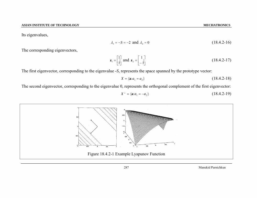
λ1 2= − = −S and 02 =λ (18.4.2-16)

The corresponding eigenvectors,

z1

11

=⎡

⎣⎢⎤

⎦⎥ and z2

11

=−⎡

⎣⎢

⎤

⎦⎥ (18.4.2-17)

The first eigenvector, corresponding to the eigenvalue -S, represents the space spanned by the prototype vector:

X a a= ={ : }a 1 2 (18.4.2-18)

The second eigenvector, corresponding to the eigenvalue 0, represents the orthogonal complement of the first eigenvector:

X a a⊥ = = −{ : }a 1 2 (18.4.2-19)

Figure 18.4.2-1 Example Lyapunov Function


Manukid Parnichkun

288

18.4.3 Lyapunov Surface

• For the content-addressable memory network, all of the diagonal elements of the weight matrix will be equal to Q (the

number of prototype patterns).

The diagonal is zero by subtracting Q times the identity matrix,

′ = −W W IQ (18.4.3-1)

′ = − = − = −W p W I p p p pq q q q qQ S Q S Q[ ] ( ) (18.4.3-2)

• (S-Q) is an eigenvalue of W', and the corresponding eigenspace is X, the space spanned by the prototype vectors.

a ∈ X ⊥ ,

′ = − = − = −W a W I a 0 a a[ ]Q Q Q (18.4.3-3)

• -Q is an eigenvalue of W', and the corresponding eigenspace is X ⊥ .

Summary

• The eigenvectors of W' are the same as the eigenvectors of W, but the eigenvalues are (S-Q) and -Q, instead of S and

0.

• The eigenvalues of the Hessian matrix of the modified Lyapunov function,∇ ′ = − ′2V ( )a W , are -(S-Q) and Q.

• The Lyapunov function surface will have negative curvature in X and positive curvature in X ⊥ , in contrast with the

original Lyapunov function, which had negative curvature in X and zero curvature in X ⊥ .

Documents

14 Competitive Networks 14.1 Hamming Networktmr.meil.pw.edu.pl/web/content/download/5315/26431/file/neural4.pdf · Manukid Parnichkun 195 14 Competitive Networks 14.1 Hamming Network