Embed Size (px)
Citation preview

14-1
Material Requirements Planning Material Requirements Planning (MRP)(MRP)
Class Agenda: Lecture - 60 MinutesBreak - 15 MinutesProblem Solutions - 60 MinutesBreak - 15 MinutesCase Review - 45 Minutes

14-2
Requirements for Effective Use of Dependent Requirements for Effective Use of Dependent Demand Inventory ModelsDemand Inventory Models
Effective use of dependent demand inventory models requires that the operations manager know the: master production schedule specifications or bills-of-material inventory availability purchase orders outstanding lead times

14-3
The Planning ProcessThe Planning ProcessProduction Plan
Execute MaterialPlans
Master ProductionSchedule
MaterialRequirements
Plan
CapacityRequirements
Plan
Execute CapacityPlans
Realistic??No
Yes

14-4
List of components & quantities needed to make product
Provides product structure (tree) Parents: Items above given level Children: Items below given level
Shows low-level coding Lowest level in structure item occurs Top level is 0; next level is 1 etc.
Bill-of-MaterialBill-of-Material

14-5
Bicycle(1)P/N 1000
Handle Bars (1)P/N 1001
Frame Assembly (1)P/N 1002
Wheels (2)P/N 1003
Frame (1)P/N 1004
Bill-of-MaterialBill-of-Material Product Structure Tree Product Structure Tree

14-6
Manufacturing computer information system Determines quantity & timing of dependent
demand items
Material Requirements Planning Material Requirements Planning (MRP)(MRP)

14-7
Structure of the MRP SystemStructure of the MRP System
MRP by period report
MRP by date report
Planned orders report
Purchase requirements
Exception reports
MRPPrograms
Master ProductionSchedule
BOM
Lead Times
(Item Master File)
(Bill-of-Material)
Inventory Data
Purchasing data

14-8
Forecast &Firm Orders
MaterialRequirements
Planning
AggregateProductionPlanning
ResourceAvailability
MasterProductionScheduling
ShopFloor
Schedules
CapacityRequirements
PlanningRealistic?
No, modify CRP, MRP, or MPSNo, modify CRP, MRP, or MPS
YesYes
MRP and The Production Planning MRP and The Production Planning ProcessProcess

14-9
Shows items to be produced End item, customer order, module
Derived from aggregate plan
Master Production ScheduleMaster Production Schedule

14-10
Derivation of Master ScheduleDerivation of Master Schedule
Therefore, these are the gross
requirements for B10 40+10 = 50 40 50 20 15+30
= 45
1 2 3 4 5 6 7 8Periods
Gross requirements: B
Periods
10 101 2 3
Master schedule for S sold directly
40 50 15
A
CB
5 6 7 8 9 10 11
Lead time = 4 for AMaster schedule for A
40 20 30
S
B C
8 9 10 1211 13
Lead time = 6 for SMaster schedule for S

14-11
MRP DynamicsMRP Dynamics Supports “replanning”
Problem with system “nervousness”
“Time fence” - allows a segment of the master schedule to be designated as “not to be rescheduled”
“Pegging” - tracing upward in the bill-of-materials from the component to the parent item
That a manager can react to changes, doesn’t mean he/she should

14-12
MRP and JITMRP and JIT
MRP - a planning and scheduling technique with fixed lead times
JIT - a way to move material expeditiously Integrating the two:
Small bucket approach and back flushing Balanced flow approach

14-13
Lot-Sizing TechniquesLot-Sizing Techniques
Lot-for-lot - Order exactly what is needed.
Economic Order Quantity - One order quantity.
Part Period Balancing - Allow the order quantity to vary.

14-14
Order QuantityOrder Quantity
Annual CostAnnual Cost
Holding Cost Curve
Holding Cost CurveTotal Cost Curve
Total Cost Curve
Order (Setup) Cost CurveOrder (Setup) Cost Curve
Optimal Optimal Order Quantity (Q*)Order Quantity (Q*)
EOQ ModelEOQ ModelHow Much to Order?How Much to Order?

14-15
Optimal Order Quantity
Expected Number of Orders
Expected Time Between Orders Working Days / Year
Working Days / Year
= =× ×
= =
= =
=
= ×
Q*D SH
NDQ*
TN
dD
ROP d L
2
DD = Demand per year = Demand per year
SS = Setup (order) cost per order = Setup (order) cost per order
HH = Holding (carrying) cost = Holding (carrying) cost
dd = Demand per day = Demand per day
LL = Lead time in days = Lead time in days
EOQ Model EquationsEOQ Model Equations

14-16
EOQ ModelEOQ ModelWhen To OrderWhen To Order
Reorder Reorder Point Point (ROP)(ROP)
TimeTime
Inventory LevelInventory Level
AverageAverageInventory Inventory
(Q*/2)(Q*/2)
Lead TimeLead Time
Optimal Optimal Order Order QuantityQuantity(Q*)(Q*)

14-17
Part Period BalancingPart Period Balancing
• Allows the order quantity to vary to cover future requirements while balancing setup and holding costs.
• Calculates the Economic Part Period (EPP) - The period of time when the ratio of setup cost to holding cost is equal.

14-18
Extensions of MRPExtensions of MRP Closed loop MRP
- Feedback to Capacity plan, MPS
Capacity planning - load reports- Reported resource requirement in a work center.
MRP II - Material Resource Planning- Considers other resources like labor or capital
Enterprise Resource Planning- Connects all functional areas of the business

14-19
MRP in ServicesMRP in Services
Can be used when demand for service or service items is directly related to or derived from demand for other services restaurant - rolls required for each meal hospitals - implements for surgery

14-20
Distribution Resource PlanningDistribution Resource Planning
DRP requires: Gross requirements, which are the same as expected
demand or sales forecasts Minimum levels of inventory to meet customer service
levels Accurate lead times Definition of the distribution structure

14-21
Chapter 14 Problems
14.1a - Product Structure
Alpha
F(2)D(3)
14-22
51 2 3 4
Alpha
F
D
14.1b - Time Phased Product Structure
= Order or start date
6

14-23
14.1c - Gross Requirements Plan
1 2 3 4 5 6A Required 10Work Order Release 10
D Required 30D Order Release 30
F Required 20F Order Release 20

14-24
14.2 - Net Materials Plan
Lead Time Onhand Item ID 1 2 3 4 5 61 2 Alpha Gross Req 10
Sched RecProj On-hand 2 2 2 2 2 2Net Req 8Planned Rec. 8Planned Orders 8
1 4 D Gross Req 24Sched RecProj On-hand 4 4 4 4 4Net Req 20Planned Rec.Planned Orders 20
2 0 F Gross Req 16Sched RecProj On-handNet Req 16Planned Rec.Planned Orders 16

14-25
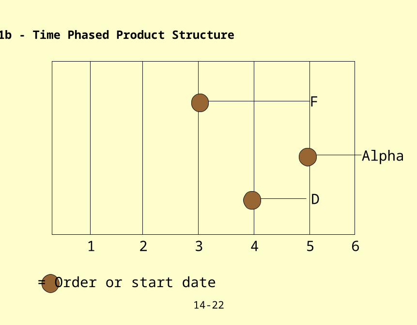
14.3a - Product Structure
S
T (1) U (2)
W (2)V (1)X (1) Z (3)Y (2)
Parent
Parent & ComponentParent & Component
All Components
14-26
61 2 3 5
S
T
U
14.3b - Time Phased Product Structure
= Order or start date
7
W
V
4
Y
Z

14-27
14.4 - Time Phased Product Structure
1 2 3 4 5 6 7S Required 100Work Order Release 100
T Required 100T Order Release 100
U Required 200U Order Release 200
V Required 100V Order Release 100
W Required 200W Order Release 200
X Required 100X Order Release 100
Y Required 400Y Order Release 400
Z Required 600Z Order Release 600

14-28
14.5 - Net Material Requirements
Lead Time Onhand Item ID 1 2 3 4 5 6 7
2 20 S Gross Req 100Sched RecProj On-hand 20 20 20 20 20 20 20Net Req 80Planned Rec.Planned Orders 80
1 20 T Gross Req 80Sched RecProj On-hand 20 20 20 20 20Net Req 60Planned Rec.Planned Orders 60
2 40 U Gross Req 160Sched RecProj On-hand 40 40 40 40 40Net Req 120Planned Rec.Planned Orders 120

14-29
14.5 - Continued
Lead Time Onhand Item ID 1 2 3 4 5 6
1 20 T Gross Req 80Sched RecProj On-hand 20 20 20 20 20Net Req 60Planned Rec.Planned Orders 60
2 30 V Gross Req 60Sched RecProj On-hand 30 30 30 30Net Req 30Planned Rec.Planned Orders 30
3 30 W Gross Req 120Sched RecProj On-hand 30 30 30 30Net Req 90Planned Rec.Planned Orders 90
1 25 X Gross Req 60Sched RecProj On-hand 25 25 25 25Net Req 35Planned Rec.Planned Orders 35

14-30
Lead Time Onhand Item ID 1 2 3 4 5 6
2 40 U Gross Req 160Sched RecProj On-hand 40 40 40 40 40Net Req 120Planned Rec.Planned Orders 120
2 240 Y Gross Req 240Sched RecProj On-hand 240 240 240Net Req 0Planned Rec.Planned Orders
1 40 Z Gross Req 360Sched RecProj On-hand 40 40 40Net Req 320Planned Rec.Planned Orders 320
14.5 - Continued

14-31
14.20 - EOQ
EOQ = sqr root of 2(demand)(setup cost) / carrying cost
= sqr root of (2)*275*(50) / .25 * 10
= 105
Set up cost = 3 * 50 = $150Inventory cost = (630) * .25 = $157.5
Total = $307.5
This Week 1 2 3 4 5 6 7 8 9 10
Gross Requirments 35 30 45 0 10 40 30 0 30 55Ending Inventory 0 70 40 -5 100 90 50 20 125 95 40Net RequirmentsPlanned Order Rec. 105 105 105Planned Orders 105 105 105
Reorder Point = 275/10 = 27.5 Units

14-32
14.20 - Lot for Lot
Set up cost = 8 * 50 = $400Inventory cost = 0
Total = $400
This Week 1 2 3 4 5 6 7 8 9 10
Gross Requirments 35 30 45 0 10 40 30 0 30 55Projected on Hand 0 0 0 0 0 0 0 0 0 0Net Requirments 35 30 45 0 10 40 30 0 30 55Planned Order Rec. 35 30 45 0 10 40 30 0 30 55Planned Orders 35 30 45 0 10 40 30 0 30 55

14-33
14.20 - Part Period Balancing
Set up cost = 3 * 50 = $150Inventory cost = 280 * .25 = 70
Total = $220
1 2 3 4 5 6 7 8 9 10 11Gross Requirments 35 30 45 0 10 40 30 0 30 55Projected on Hand 85 55 10 10 0 60 30 30 0 0Net RequirmentsPlanned Order Rec. 120 100 55Planned Orders 120 100 55
Holding Units (HU) 30 90 0 40 0 30 0 90 0Cummulative HU 0 30 120 120 160 0 30 30 120 0
Assumption - No carrying cost occurs during the week the order is received.
Economic Part Period = a period of time when the ratio of setup cost to holding cost is equal. EPP = 50/.25 = 200.