1336 IEEE TRANSACTIONS ON KNOWLEDGE AND … Linear Discriminant Analysis Technique for Dimensionality Reduction Alok Sharma, Member, IEEE, and Kuldip K. Paliwal,Member, IEEE Abstract—The

Rotational Linear Discriminant AnalysisTechnique for Dimensionality Reduction

Alok Sharma, Member, IEEE, and Kuldip K. Paliwal, Member, IEEE

Abstract—The linear discriminant analysis (LDA) technique is very popular in pattern recognition for dimensionality reduction. It is a

supervised learning technique that finds a linear transformation such that the overlap between the classes is minimum for the projected

feature vectors in the reduced feature space. This overlap, if present, adversely affects the classification performance. In this paper,

we introduce prior to dimensionality-reduction transformation an additional rotational transform that rotates the feature vectors in the

original feature space around their respective class centroids in such a way that the overlap between the classes in the reduced feature

space is further minimized. As a result, the classification performance significantly improves, which is demonstrated using several data

corpuses.

Index Terms—Rotational linear discriminant analysis, dimensionality reduction, classification error, fixed-point algorithm, probability of

error.

Ç

1 INTRODUCTION

IN a typical pattern recognition application, some char-

acteristic properties (or features) of an object aremeasured, and the resulting feature vector is classified into

one of the finite number of classes. When the number of

features is relatively large, it becomes difficult to train a

classifier using a finite amount of training data. In addition,

the complexity of a classifier increases with the number of

features used. In such situations, it becomes important to

reduce the dimensionality of the feature space. There are a

number of techniques proposed in the literature fordimensionality reduction [3], [7], [9]; the linear discriminant

analysis (LDA) technique [7] is perhaps the most popular

among them. LDA is a supervised learning technique that

uses a linear transformation to project the feature vectors

from the original feature space to a subspace in such a way

that the overlap between the classes is minimized in the

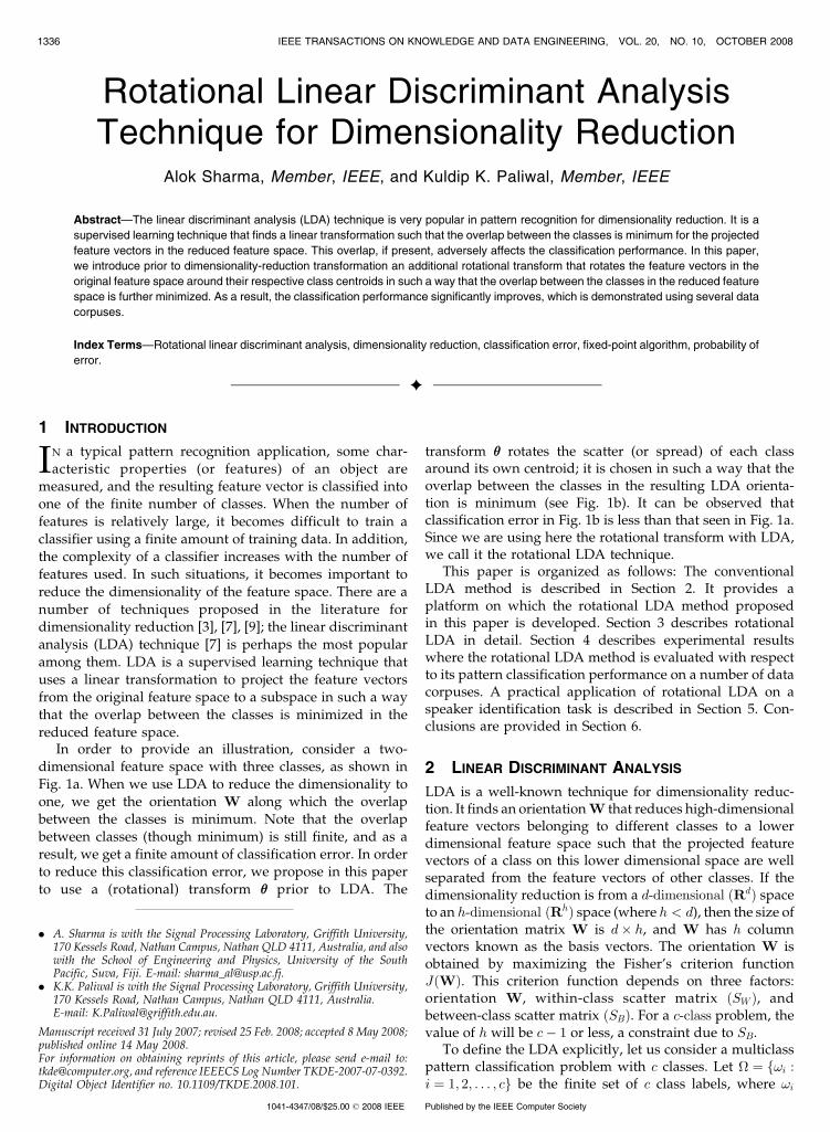
reduced feature space.In order to provide an illustration, consider a two-

dimensional feature space with three classes, as shown in

Fig. 1a. When we use LDA to reduce the dimensionality toone, we get the orientation W along which the overlapbetween the classes is minimum. Note that the overlap

between classes (though minimum) is still finite, and as aresult, we get a finite amount of classification error. In orderto reduce this classification error, we propose in this paper

to use a (rotational) transform �� prior to LDA. The

transform �� rotates the scatter (or spread) of each classaround its own centroid; it is chosen in such a way that theoverlap between the classes in the resulting LDA orienta-tion is minimum (see Fig. 1b). It can be observed thatclassification error in Fig. 1b is less than that seen in Fig. 1a.Since we are using here the rotational transform with LDA,we call it the rotational LDA technique.

This paper is organized as follows: The conventionalLDA method is described in Section 2. It provides aplatform on which the rotational LDA method proposedin this paper is developed. Section 3 describes rotationalLDA in detail. Section 4 describes experimental resultswhere the rotational LDA method is evaluated with respectto its pattern classification performance on a number of datacorpuses. A practical application of rotational LDA on aspeaker identification task is described in Section 5. Con-clusions are provided in Section 6.

2 LINEAR DISCRIMINANT ANALYSIS

LDA is a well-known technique for dimensionality reduc-tion. It finds an orientation W that reduces high-dimensionalfeature vectors belonging to different classes to a lowerdimensional feature space such that the projected featurevectors of a class on this lower dimensional space are wellseparated from the feature vectors of other classes. If thedimensionality reduction is from a d-dimensional ðRdÞ spaceto an h-dimensional ðRhÞ space (where h < d), then the size ofthe orientation matrix W is d� h, and W has h columnvectors known as the basis vectors. The orientation W isobtained by maximizing the Fisher’s criterion functionJðWÞ. This criterion function depends on three factors:orientation W, within-class scatter matrix ðSW Þ, andbetween-class scatter matrix ðSBÞ. For a c-class problem, thevalue of h will be c� 1 or less, a constraint due to SB.

To define the LDA explicitly, let us consider a multiclasspattern classification problem with c classes. Let � ¼ f!i :i ¼ 1; 2; . . . ; cg be the finite set of c class labels, where !i

1336 IEEE TRANSACTIONS ON KNOWLEDGE AND DATA ENGINEERING, VOL. 20, NO. 10, OCTOBER 2008

. A. Sharma is with the Signal Processing Laboratory, Griffith University,170 Kessels Road, Nathan Campus, Nathan QLD 4111, Australia, and alsowith the School of Engineering and Physics, University of the SouthPacific, Suva, Fiji. E-mail: [email protected].

. K.K. Paliwal is with the Signal Processing Laboratory, Griffith University,170 Kessels Road, Nathan Campus, Nathan QLD 4111, Australia.E-mail: [email protected].

Manuscript received 31 July 2007; revised 25 Feb. 2008; accepted 8 May 2008;published online 14 May 2008.For information on obtaining reprints of this article, please send e-mail to:[email protected], and reference IEEECS Log Number TKDE-2007-07-0392.Digital Object Identifier no. 10.1109/TKDE.2008.101.

1041-4347/08/$25.00 � 2008 IEEE Published by the IEEE Computer Society

denotes the ith class label. Let �� ¼ fxj 2 Rd; j ¼ 1; . . . ; ngdenote the set of n training samples (or feature vectors) in

a d-dimensional space. The set �� can be subdivided into

c subsets ��1; ��2; . . . ; ��c, where each subset ��i belongs to !iand consists of ni feature vectors such that n ¼

Pci¼1 ni and

��1 [ ��2[; . . . ;[��c ¼ ��.Let ��j be the centroid of ��j and �� be the centroid of ��,

then the between-class scatter matrix ðSBÞ is given as

SB ¼Xcj¼1

njð��j � ��Þð��j � ��ÞT:

The within-class scatter matrix ðSW Þ, which is the sum of c

scatter matrices, is defined as

SW ¼Xci¼1

Mi;

where Mi ¼P

x2�iðx� ��iÞðx� ��iÞT.

Fisher’s criterion as a function of W can be given as [7]

JðWÞ ¼ jWTSBWj

jWTSWWj;

where j � j is the determinant. The orientation W is taken sothat the Fisher’s criterion function JðWÞ is maximum. In ac-class problem, the LDA projects from a d-dimensionalspace to an h-dimensional space; i.e., W : x! y, ory ¼WTx, where x 2 Rd and y 2 Rh such that 1 � h �c� 1. The orientation W is a rectangular matrix of sized� h, which is the solution of the eigenvalue problem:

S�1W SBwi ¼ �iwi;

where wi are the column vectors of W that correspond tothe largest eigenvalues ð�iÞ.

In the conventional LDA technique, the Gaussianassumption is not required. However, the within-classscatter matrix ðSW Þ needs to be nonsingular. When thenumber of training samples is not adequate, this scattermatrix becomes singular. This occurs especially when theoriginal feature space is very high. This drawback isconsidered to be the main problem of LDA and is knownas the small sample size (SSS) problem [9]. The SSS problemhas generated widespread interest among researchers, anda number of computational methods have been proposed inthe literature to overcome this problem.

A simple and direct way to avoid the singularity problemis to replace the inverse of the within-class matrix by itspseudoinverse [19], [25]. However, this does not guaranteethe optimality of Fisher’s criterion. Another way to overcomethe singularity problem is through the regularized LDAmethod [8], [11], [16], which adds a small positive constant tothe diagonal elements of SW to make it nonsingular. Thismethod is also suboptimal as Fisher’s criterion is not exactlymaximized. Swets and Weng [24] and Belhumeur et al. [2]have proposed a two-stage method (known as the Fisherfacemethod) to avoid the singularity problem. In the first stage,the principal component analysis (PCA) is used fordimensionality reduction in such a way that the within-classmatrix in the reduced dimensional subspace becomesnonsingular. In the second stage, the classical LDA is usedto reduce the dimensionality further. The two-stage Fisher-face method (also known as the PCA+LDA method) issuboptimal as the PCA used in the first-stage loses somediscriminative information. In order to avoid this loss indiscriminative information, two other recently proposedtwo-stage methods to overcome the SSS problem are the nullspace method [6] and the direct LDA method [28]. In the nullspace method, the first stage transforms the training datavectors to the null space of the within-class scatter matrix SW(i.e., it discards the range space of SW ). In the second stage,the dimensionality is reduced by choosing h eigenvectors ofthe transformed between-class scatter matrix correspondingto the highest eigenvalues. In the direct LDA method, thefirst stage discards the null space of the between-class scattermatrix SB (i.e., the training data vectors are transformed intothe range space of SB), and the second stage reduces thedimensionality to h by choosing h eigenvectors of thetransformed within-class scatter matrix corresponding tothe lowest eigenvalues. Though these two-stage methods(the null space method and the direct LDA method) providebetter classification performance than the PCAþLDAmethod, these are still suboptimum as they optimize Fisher’scriterion sequentially in two stages.

SHARMA AND PALIWAL: ROTATIONAL LINEAR DISCRIMINANT ANALYSIS TECHNIQUE FOR DIMENSIONALITY REDUCTION 1337

Fig. 1. A comparison between basic LDA and rotational LDA techniques.

Here, we have provided a brief overview of some of theLDA methods to overcome the SSS problem; for othermethods, see [5], [17], [18], [23], and [27]. It is important tonote that though these methods overcome the SSS problem,they do not ensure the optimality of Fisher’s criterion as donein the conventional LDA method and hence are suboptimal.

3 ROTATIONAL LINEAR DISCRIMINANT ANALYSIS

3.1 Theory

This section provides the mathematical details of therotational LDA method. Let us consider a multiclass patternclassification problem with c classes. Let � ¼ f!i : i ¼1; 2; . . . ; cg be the finite set of c class labels. Let �� ¼ fxj 2Rd; j ¼ 1; . . . ; ng denote the set of n training samples (orfeature vectors) in d-dimensional space.

Let �Yj 2 Rh (where h < d) be the reduced h-dimensionalfeature vector obtained from ��j 2 !j using LDA transfor-mation and denote the set of reduced dimensionalfeature vectors by �Y ¼ fy1;y2; . . . ;yng. Thus, �Yj � �Y ,and �Y1 [ �Y2 [ � � � [ �Yc ¼ �Y .

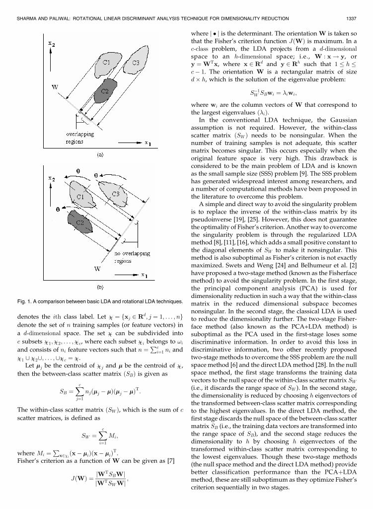
For illustration, consider a two-class problem ðc ¼ 2Þ asshown in Fig. 2, where ��1 and ��2 are the two subsets offeature vectors in the original two-dimensional spaceðx 2 R2Þ. The class labels of these subsets are representedas !1 and !2, respectively. This original space is transformedto a lower one-dimensional subspace ðy 2 R1Þ, producingtransformed sample sets�Y1 and�Y2, which belong to the classlabels !1 and !2, respectively. The transformation is con-ducted using an LDA transformation W of size d� h (in thisillustration, h ¼ 1); i.e., W : x! y, or yj ¼WTxj forj ¼ 1; . . . ; n. The respective probability distributions of �Y1

and �Y2 are also shown in Fig. 2. The classifier divides theone-dimensional subspace into two regionsR��1 andR��2. Thereare two possibilities in which a classification error couldoccur; either observation yðW : x! yÞ falls in the region R��1

and the true class is !2 or y falls in the regionR��2 and the trueclass is !1. Since these events are mutually exclusive andexhaustive [7], we can define probability of error as

Perror ¼ P ðy 2 !2; R��1Þ þ P ðy 2 !1; R��2Þ¼ P ðy 2 R��1j!2ÞP ð!2Þ þ P ðy 2 R��2j!1ÞP ð!1Þ

¼Z

y2R�1

pðyj!2ÞP ð!2ÞdyþZ

y2R�2

pðyj!1ÞP ð!1Þdy;

where P ð!jÞ is the a priori probability of �Yj. In a multiclasscase, it would be easier to find the probability of beingcorrect [7]. Therefore

Pcorrect ¼Xcj¼1

Zy2R�j

pðyj!jÞP ð!jÞdy:

We can also compute the total probability of �Y byevaluating the probability densities separately for each of�Yj and finally adding the computed densities; i.e.

Ptotal ¼Xcj¼1

Zy2�Yj

pðyj!jÞpð!jÞdy:

The Ptotal function is independent of regions R��j; therefore,it will remain unchanged with respect to the values of R��j. Itcan be observed that Pcorrect and Perror add up together togive Ptotal; i.e.

Ptotal ¼ Pcorrectþ Perror:

Therefore, the probability error function can be written as

Perror ¼ b� Pcorrect

¼ b�Xcj¼1

Zy2R�j

pðyj!jÞP ð!jÞdy; ð1Þ

where b is a constant and is equal to Ptotal. In practice, wehave to compute the integral in (1) using the data in thetraining set. Therefore, we approximate the integrationoperation by a summation operation as follows [1]:

A ¼ZfðxÞdx ¼ lim

n!1

Xnk¼1

fðxkÞ�x �Xnk¼1

fðxkÞ�x: ð2Þ

Using this approximation (2), (1) can be rewritten as

Perror ¼ b�Xcj¼1

Xy2R�j

pðyj!jÞP ð!jÞ�V ; ð3Þ

where �V is a volume of a tiny hypercube. This �V is ascalar quantity and depends upon the transformedsample set �Y . Equation (3) is a probability error functionfor a scalar y, which can be extended to vector y simplyby replacing a vector in place of scalar y.

Constant �V is independent of any class and therefore istaken outside from the summations of (3). The value of apriori probability P ð!jÞ ¼ nj=n is substituted in (3); thisyields Perror as

Perror ¼ b� kXcj¼1

njXy2R�j

pðyj!jÞ; ð4Þ

where k ¼ �V =n is a constant.The basic LDA transformation ðy ¼WTxÞ has to be

changed to account for the rotation of the original space. Weintroduce a rotational transform �� prior to LDA and trans-form the feature vector x belonging to class !j as follows:

y ¼WT ��Tðx� ��xjÞ þ ��xj

h i; ð5Þ

where ��xjis the mean of ��j.


Fig. 2. Probability error for the two-class problem.

At the beginning when no rotation has taken place, thetransformation �� would be a d� d identity matrix, and (5)would reduce to the basic LDA transformation. To findthe optimum rotation ��, it is required to differentiate thescalar function (4) with respect to the transformationmatrix ��. The value of �� that corresponds to theminimum of Perror would be the optimum rotation ��.From (4), we get

@

@��Perror ¼ �k

Xcj¼1

njXy2R�j

@

@��pðyj!jÞ; ð6Þ

where y is from (5). The next thing is to find theprobability distribution pðyj!jÞ before differentiating itwith respect to ��. One way to estimate pðyj!jÞ is to use aparametric technique where we assume a functional formof the distribution characterized by a few parameters.Here, we assume y to be distributed as multidimensionalGaussian.1 Differentiating the resulting pðyj!jÞ, we get

@

@��pðyj!jÞ ¼

@

@��

(1

ð2�Þh=2 �yj

�� 1=2

exp � 1

2y� ��yj

� �T��1

yjy� ��yj

� �� );

ð7Þ

where ��yjand ��yj are the mean and the covariance of �Yj.

Substituting (5) in (7), we get

@

@�pðyj!jÞ

¼ @

@�pðx; ��;Wj!jÞ

¼ @

@��

(1

ð2�Þh=2 �yj

�� 1=2

exp � 1

2x��xj

� �T��W��1

yjWT��T x��xj

� �� );

ð8Þ

where x is the corresponding vector of y 2 R��j; i.e., vectorsx 2 ��j are used to compute y 2 R��j (using (5)) in (8). Let usrepresent this correspondence relation by xðy 2 R��jÞ. Thefollowing lemma would help in solving (8).

Lemma 1. Let the scalar function expð� 12uÞ be a differentiable

function of a d� d square matrix ��. Suppose

u ¼ ��T��WBWT��T��;

where �� is any vector of size d� 1, B is a square matrixof size h� h, and W is a rectangular matrix of size d� hsuch that h < d. It can be assumed that both the matrices(B and W) and the vector ð��Þ are independent of ��.Then, the gradient of expð� 1

2uÞ is defined asr��expð� 1

2uÞ ¼ � 12 expð� 1

2 uÞ��T��WðBþBTÞWT.

Proof 1. The derivative of scalar expð� 12 uÞ with respect to

matrix �� can be given as

@ exp � 1

2u

� �

¼ � 1

2exp � 1

2u

� �trace @ð��T��WBWT��T��Þ

� �¼ � 1

2exp � 1

2u

� �ntrace½��T@ ��WBWT��T��Þ

þ trace½��T��WBWT@ ��T��o

¼ � 1

2exp � 1

2u

� �ntrace½��T�� WBTWT@ ��T��Þ

þ trace½��T��WBWT@ ��T��o

� �� trðAT Þ ¼ trðAÞ

� �¼ � 1

2exp � 1

2u

� �trace ��T��WðBþBTÞWT@ ��T��Þ

� � ¼ � 1

2exp � 1

2u

� �trace ��T��WðBþBTÞWT@ ��TÞ

� � � �� trðADÞ ¼ trðDAÞ

� �� r��exp � 1

2u

� �¼ � 1

2exp � 1

2u

� ��T��WðBþBTÞWT:

tu

Using Lemma 1, we can rewrite (8) as

@

@��pðyj!jÞ ¼ � 1

2ð2�Þh=2j�yj j1=2

exp � 1

2u

� �" #

� x� ��xj

� �x� ��xj

� �T��W ��1

yjþ��1

yj

T� �

WT

� �;

ð9Þ

where u ¼ ðx� ��xjÞT��W��1

yjWT��Tðx� ��xj

Þ. Substituting

(9) in (6), we get

@

@��Perror ¼ k0

Xcj¼1

nj

j�yj j1=2

Xxðy2R�jÞ

exp � 1

2u

� �

� x��xj

� �x��xj

� �T��W ��1

yjþ��1

yj

T� �

WT

� �;

ð10Þ

where k0 ¼ k=ð2ð2�Þh=2Þ. Equation (10) can also be written in

the expectation form as

@

@��Perror ¼ k0

Xcj¼1

n2j

�yj

�� 1=2 Exðy2R�jÞ

F x; ��;W; ��xj;�yj

� �h i;

where

F x; ��;W; ��xj;�yj

� �¼ exp � 1

2u

� ��

��

x� �xj

� �x� ��xj

� �T��W

� ��1yjþ��1

yj

T� �

WT

�;

and E½F ð�Þ is the expectation of Fð�Þ with respect to x.


1. It should be noted that the class-conditional probability densityfunction pðyj!jÞ is assumed here to be a multidimensional Gaussianfunction for analytical simplicity purposes. But this choice is justifiable fromthe central limit theorem as y is computed from x through a lineartransformation (see (5)).

Since the topography of the original data should remainunchanged during rotation ��, the column vectors of ��

should be orthonormal. This means that the square matrix ��is orthonormal; i.e., ��T�� ¼ Id�d. This allows us to use a fixed-point algorithm [14], which is known to be faster and morereliable than the gradient algorithms. The fixed-pointalgorithm for rotation �� is written as follows:

�� /Xcj¼1

n2j

�yj

�� 1=2E

xðy2R�jÞF x; ��;W; ��xj

;�yj

� �h i; ð11Þ

�� ð��T��Þ�1=2: ð12Þ

The values of W and �yj will be changing depending uponthe rotation of the original feature space, whereas the classcentroid ��xj

will remain invariant for any such rotationsince the rotation of the training vectors of a class is alwayswith respect to its centroid ��xj

. The matrices W and ��yj

should be updated for every iteration of �� for (11). Theinverse of ��T�� in (12) is computed using eigenvalue

decomposition. There are iterative methods for orthonor-malization that avoid the matrix inverse and eigendecom-position. In that case, the rotation matrix �� can beorthonormalized by using a symmetric orthonormalizationprocedure starting from a nonorthogonal matrix andcontinuing the iterative process until ��T�� Id�d [13].

The value of Perror can be estimated more economicallyalso for each of the iteration of (11) and (12) by applying thefollowing equation instead of applying (1):

Perror ¼ 1�

Pcj¼1

number of samples belongs to R��j given !j

total number of samples in ��

¼ 1�

Pcj¼1

ðnjjR��j; !jÞ

n;

ð13Þ

where ðnjjR��j; !jÞ denotes the number of samples thatbelong to the jth region ðR��jÞ given class label !j. Region R��jof the training samples can be obtained by several methods.We have used the nearest neighbor classifier (with squaredeuclidean distance measure) for finding the regions.

3.2 Training Phase of Rotational LDA

The previous section has provided a mathematical descrip-tion of the rotational LDA method. In this section, weprovide its algorithmic description. As mentioned earlier,the rotational LDA algorithm is iterative in nature. It isgiven in Table 1. This algorithm computes parameters ��, W,and ��yj

ðj ¼ 1; . . . ; cÞ (listed in Table 2) from the trainingdata as follows:

Prior to the iterative process, compute ��xj2 Rd ðj ¼

1; . . . ; cÞ from the training data and initialize the rotation ��by a d� d identity matrix. In the first iteration, the firststep is to find the orientation W (using �� to be the identitymatrix from the initialization step) by applying the basicLDA procedure. The obtained orientation W will be suchthat the overlap between classes is minimum in thereduced dimensional space (i.e., W maximizes Fisher’scriterion). This transformation may produce overlappingof samples in the reduced dimensional space betweenadjacent classes that cannot be reduced any further bymoving the direction (orientation) W around the origin inthe reduced dimensional feature space. Let P1 be the errorwith computed W and �� from the previous iteration. Inthe second step, compute the rotation �� in the originalfeature space using the fixed-point algorithm. By applyingthis rotation �� in the original feature space, we get areduced dimensional feature space with much less over-lapping between the adjacent classes. With this ��, we go


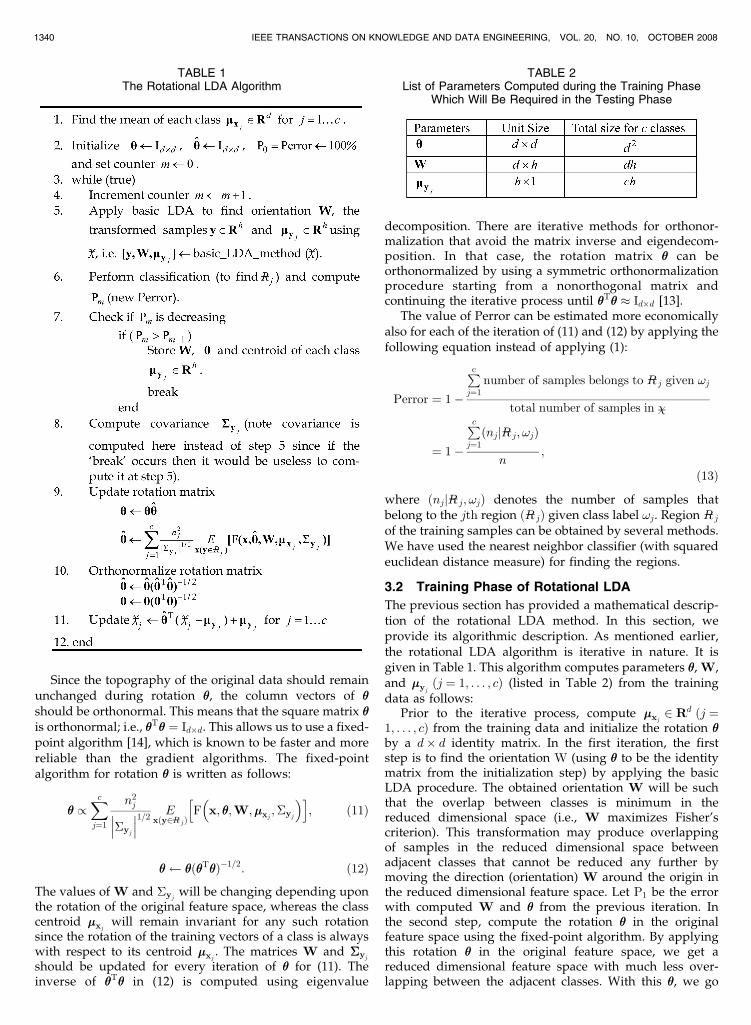
TABLE 1The Rotational LDA Algorithm

TABLE 2List of Parameters Computed during the Training Phase

Which Will Be Required in the Testing Phase

to the second iteration and compute W in the first step(which gives error P2 < P1) and �� in the second step. Thisiterative process is continued as long as the reduction inerror between successive iterations is significant. For thedata sets used in this paper, we have observed that thisalgorithm needs only a few iterations (typically two tofour) to converge.

We know that the rotational LDA algorithm is an

iterative algorithm, and it rotates the original featurevectors with respect to the centroid of their own class

separately, until the minimum overlapping error is ob-

tained. It would be interesting to see what happens to theoriginal feature vectors x 2 ��j 2 Rd after the mth iteration

of the algorithm. Let us denote the rotated feature vectors

after the first iteration as x1. It can then be expressed interms of the original feature vectors x as

Iteration 1 : x1 ¼ ��T1 x� ��xj

� �þ ��xj

: ð14Þ

After the second iteration, the feature vectors would be

Iteration 2 : x2 ¼ ��T2 x1 � ��xj

� �þ ��xj

: ð15Þ

Similarly, after the mth iteration, feature vectors can be

given as

Iteration m : xm ¼ ��Tm xm�1 � ��xj

� �þ ��xj

: ð16Þ

It should be noted that the location of the centroid of a classis not changing since the rotation of feature vectors is

always with respect to the centroid of their own class.Substituting (14) in (15), we get

x2 ¼ ��T2 ��

T1 x� ��xj

� �þ ��xj

:

Similarly, we can say that

xm ¼ ��Tm . . . ��T

2 ��T1 x� ��xj

� �þ ��xj

;

or

xm ¼ ��Tðx� ��xjÞ þ ��xj

;

where �� ¼ ��1; ��2; . . . ; ��m. Some issues related to the compu-tational complexity of the training phase are discussed inthe Appendix.

3.3 An Example of the Training Phase ofRotational LDA

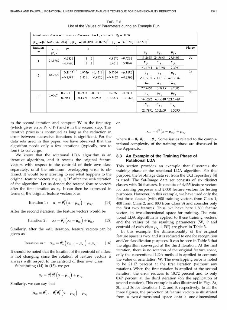
This section provides an example that illustrates thetraining phase of the rotational LDA algorithm. For thispurpose, the Sat-Image data set from the UCI repository [4]is used. The Sat-Image data set consists of six distinctclasses with 36 features. It consists of 4,435 feature vectorsfor training purposes and 2,000 feature vectors for testingpurposes. However, in this example, we have used only thefirst three classes (with 600 training vectors from Class 1,400 from Class 2, and 800 from Class 3) and consider onlythe first two features. Thus, we have here 1,800 featurevectors in two-dimensional space for training. The rota-tional LDA algorithm is applied to these training vectors,and the values of the resulting parameters (W, �� andcentroid of each class ��yj

2 Rh) are given in Table 3.In this example, the dimensionality of the original

feature space is two, and it is reduced to one for recognitionand/or classification purposes. It can be seen in Table 3 thatthe algorithm converged at the third iteration. At the firstiteration, there is no rotation of the original feature space,only the conventional LDA method is applied to computethe value of orientation W. The overlapping error is notedto be 21.17 percent at the first iteration (without anyrotation). When the first rotation is applied at the seconditeration, the error reduces to 18.72 percent and to only0.67 percent at the third iteration (on the application ofsecond rotation). This example is also illustrated in Figs. 3a,3b, and 3c for iterations 1, 2, and 3, respectively. In all thethree figures, the projection of feature vectors is illustratedfrom a two-dimensional space onto a one-dimensional


TABLE 3List of the Values of Parameters during an Example Run

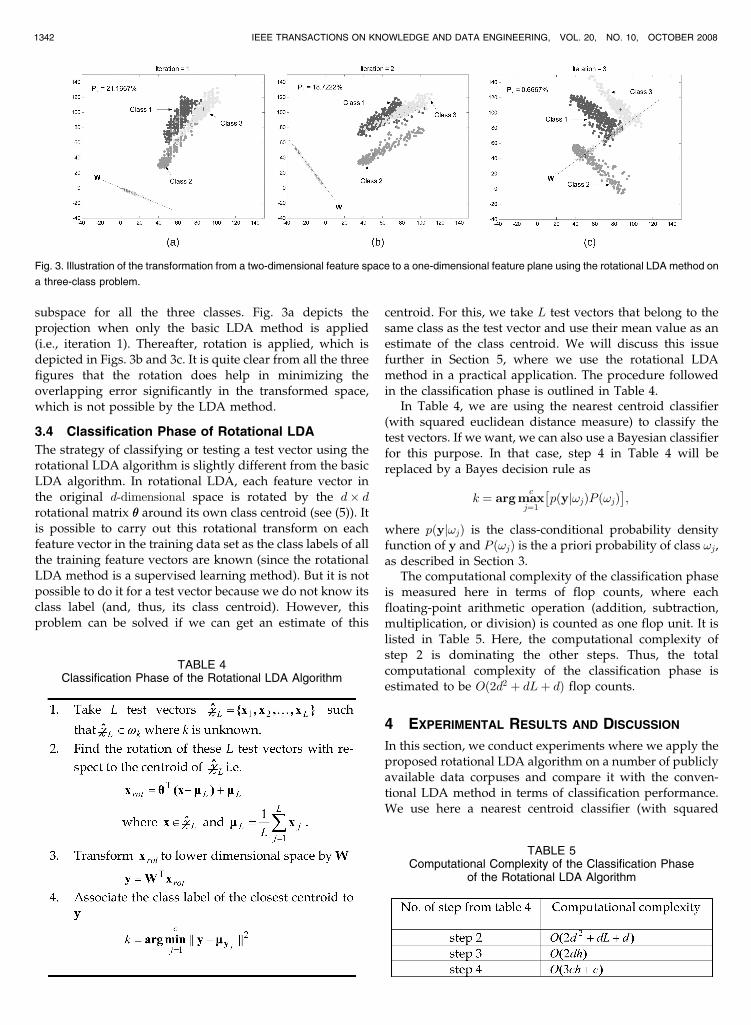
subspace for all the three classes. Fig. 3a depicts theprojection when only the basic LDA method is applied(i.e., iteration 1). Thereafter, rotation is applied, which isdepicted in Figs. 3b and 3c. It is quite clear from all the threefigures that the rotation does help in minimizing theoverlapping error significantly in the transformed space,which is not possible by the LDA method.

3.4 Classification Phase of Rotational LDA

The strategy of classifying or testing a test vector using therotational LDA algorithm is slightly different from the basicLDA algorithm. In rotational LDA, each feature vector inthe original d-dimensional space is rotated by the d� drotational matrix �� around its own class centroid (see (5)). Itis possible to carry out this rotational transform on eachfeature vector in the training data set as the class labels of allthe training feature vectors are known (since the rotationalLDA method is a supervised learning method). But it is notpossible to do it for a test vector because we do not know itsclass label (and, thus, its class centroid). However, thisproblem can be solved if we can get an estimate of this

centroid. For this, we take L test vectors that belong to thesame class as the test vector and use their mean value as anestimate of the class centroid. We will discuss this issuefurther in Section 5, where we use the rotational LDAmethod in a practical application. The procedure followedin the classification phase is outlined in Table 4.

In Table 4, we are using the nearest centroid classifier(with squared euclidean distance measure) to classify thetest vectors. If we want, we can also use a Bayesian classifierfor this purpose. In that case, step 4 in Table 4 will bereplaced by a Bayes decision rule as

k ¼ arg maxc

j¼1pðyj!jÞP ð!jÞ� �

;

where pðyj!jÞ is the class-conditional probability densityfunction of y and P ð!jÞ is the a priori probability of class !j,as described in Section 3.

The computational complexity of the classification phaseis measured here in terms of flop counts, where eachfloating-point arithmetic operation (addition, subtraction,multiplication, or division) is counted as one flop unit. It islisted in Table 5. Here, the computational complexity ofstep 2 is dominating the other steps. Thus, the totalcomputational complexity of the classification phase isestimated to be Oð2d2 þ dLþ dÞ flop counts.

4 EXPERIMENTAL RESULTS AND DISCUSSION

In this section, we conduct experiments where we apply theproposed rotational LDA algorithm on a number of publiclyavailable data corpuses and compare it with the conven-tional LDA method in terms of classification performance.We use here a nearest centroid classifier (with squared


Fig. 3. Illustration of the transformation from a two-dimensional feature space to a one-dimensional feature plane using the rotational LDA method on

a three-class problem.

TABLE 4Classification Phase of the Rotational LDA Algorithm

TABLE 5Computational Complexity of the Classification Phase

of the Rotational LDA Algorithm

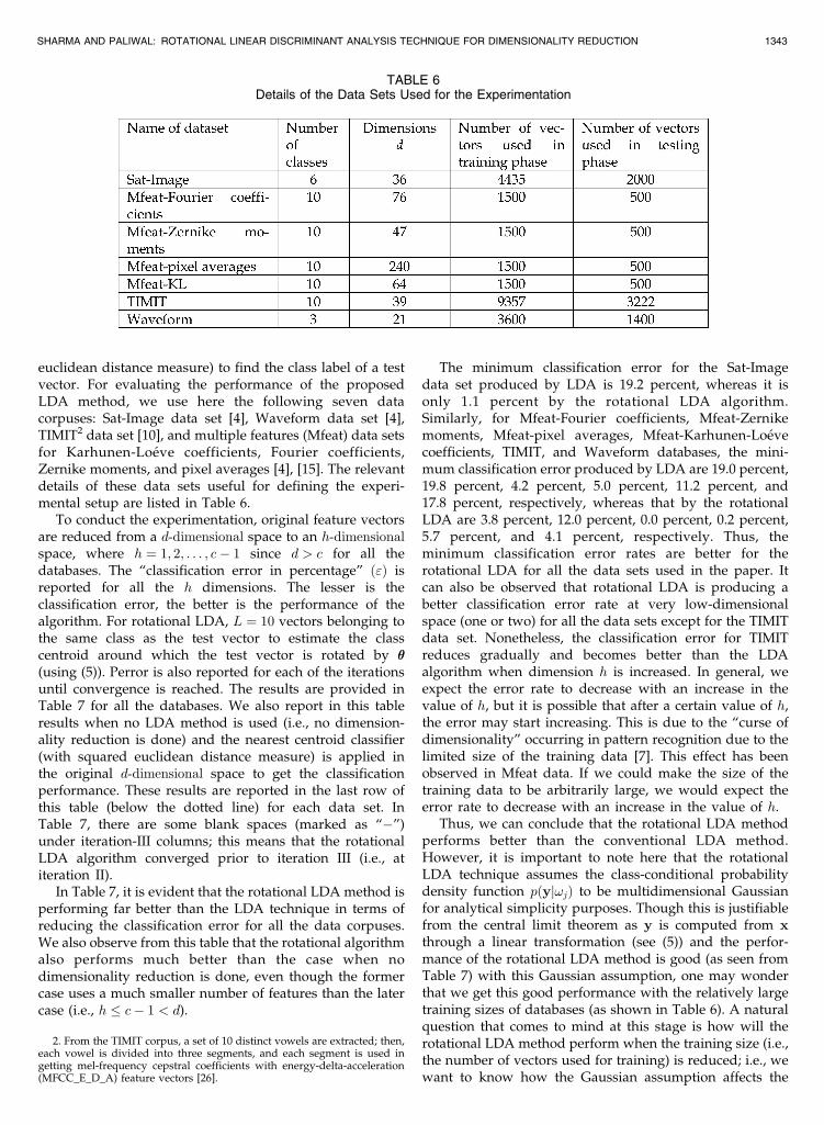
euclidean distance measure) to find the class label of a testvector. For evaluating the performance of the proposedLDA method, we use here the following seven datacorpuses: Sat-Image data set [4], Waveform data set [4],TIMIT2 data set [10], and multiple features (Mfeat) data setsfor Karhunen-Loeve coefficients, Fourier coefficients,Zernike moments, and pixel averages [4], [15]. The relevantdetails of these data sets useful for defining the experi-mental setup are listed in Table 6.

To conduct the experimentation, original feature vectorsare reduced from a d-dimensional space to an h-dimensionalspace, where h ¼ 1; 2; . . . ; c� 1 since d > c for all thedatabases. The “classification error in percentage” ð"Þ isreported for all the h dimensions. The lesser is theclassification error, the better is the performance of thealgorithm. For rotational LDA, L ¼ 10 vectors belonging tothe same class as the test vector to estimate the classcentroid around which the test vector is rotated by ��(using (5)). Perror is also reported for each of the iterationsuntil convergence is reached. The results are provided inTable 7 for all the databases. We also report in this tableresults when no LDA method is used (i.e., no dimension-ality reduction is done) and the nearest centroid classifier(with squared euclidean distance measure) is applied inthe original d-dimensional space to get the classificationperformance. These results are reported in the last row ofthis table (below the dotted line) for each data set. InTable 7, there are some blank spaces (marked as “�”)under iteration-III columns; this means that the rotationalLDA algorithm converged prior to iteration III (i.e., atiteration II).

In Table 7, it is evident that the rotational LDA method isperforming far better than the LDA technique in terms ofreducing the classification error for all the data corpuses.We also observe from this table that the rotational algorithmalso performs much better than the case when nodimensionality reduction is done, even though the formercase uses a much smaller number of features than the latercase (i.e., h � c� 1 < d).

The minimum classification error for the Sat-Imagedata set produced by LDA is 19.2 percent, whereas it isonly 1.1 percent by the rotational LDA algorithm.Similarly, for Mfeat-Fourier coefficients, Mfeat-Zernikemoments, Mfeat-pixel averages, Mfeat-Karhunen-Loevecoefficients, TIMIT, and Waveform databases, the mini-mum classification error produced by LDA are 19.0 percent,19.8 percent, 4.2 percent, 5.0 percent, 11.2 percent, and17.8 percent, respectively, whereas that by the rotationalLDA are 3.8 percent, 12.0 percent, 0.0 percent, 0.2 percent,5.7 percent, and 4.1 percent, respectively. Thus, theminimum classification error rates are better for therotational LDA for all the data sets used in the paper. Itcan also be observed that rotational LDA is producing abetter classification error rate at very low-dimensionalspace (one or two) for all the data sets except for the TIMITdata set. Nonetheless, the classification error for TIMITreduces gradually and becomes better than the LDAalgorithm when dimension h is increased. In general, weexpect the error rate to decrease with an increase in thevalue of h, but it is possible that after a certain value of h,the error may start increasing. This is due to the “curse ofdimensionality” occurring in pattern recognition due to thelimited size of the training data [7]. This effect has beenobserved in Mfeat data. If we could make the size of thetraining data to be arbitrarily large, we would expect theerror rate to decrease with an increase in the value of h.

Thus, we can conclude that the rotational LDA methodperforms better than the conventional LDA method.However, it is important to note here that the rotationalLDA technique assumes the class-conditional probabilitydensity function pðyj!jÞ to be multidimensional Gaussianfor analytical simplicity purposes. Though this is justifiablefrom the central limit theorem as y is computed from xthrough a linear transformation (see (5)) and the perfor-mance of the rotational LDA method is good (as seen fromTable 7) with this Gaussian assumption, one may wonderthat we get this good performance with the relatively largetraining sizes of databases (as shown in Table 6). A naturalquestion that comes to mind at this stage is how will therotational LDA method perform when the training size (i.e.,the number of vectors used for training) is reduced; i.e., wewant to know how the Gaussian assumption affects the


2. From the TIMIT corpus, a set of 10 distinct vowels are extracted; then,each vowel is divided into three segments, and each segment is used ingetting mel-frequency cepstral coefficients with energy-delta-acceleration(MFCC_E_D_A) feature vectors [26].

TABLE 6Details of the Data Sets Used for the Experimentation

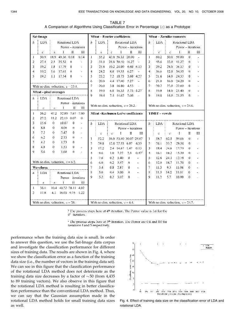
performance when the training data size is small. In orderto answer this question, we use the Sat-Image data corpusand investigate the classification performance for differentsizes of training data. The results are shown in Fig. 4, wherewe show the classification error as a function of the trainingdata size (i.e., the number of vectors in the training data set).We can see in this figure that the classification performanceof the rotational LDA method does not deteriorate as thetraining data size decreases by a factor of 50 (from 4,435to 89 training vectors). We also observe in this figure thatthe rotational LDA method is resulting in better classifica-tion performance than the conventional LDA method. Thus,we can say that the Gaussian assumption made in therotational LDA method holds for small training data sizesas well.


TABLE 7A Comparison of Algorithms Using Classification Error in Percentage ð"Þ as a Prototype

Fig. 4. Effect of training data size on the classification error of LDA and

rotational LDA.

5 A PRACTICAL APPLICATION OF ROTATIONAL

LDA: SPEAKER IDENTIFICATION

In this section, we illustrate the practical application of therotational LDA method in text-dependent speaker identifi-cation. A speaker identification system [12] uses the speechutterance of a person (who speaks a prespecified keywordor sentence) to find his/her identity from a group ofprerecorded persons. The speech utterance is analyzedframewise, and an acoustic front end is used to measure afew characteristic properties (or features) from the signal ofeach frame. In the current state-of-the-art speaker identifi-cation systems, the mel frequency cepstral coefficients(MFCCs) are commonly used as features [12], [20]. Thus, aframe is represented by a d-dimensional feature vector withd MFCCs as its components. In the experiment reported inthis section, the speaker identification system makes adecision about the speaker’s identity for each frame.

In the rotational LDA method, a test vector that we wantto classify is rotated around the centroid of its own class.Since the information about the class centroid is not known(as we do not know to which class the test vector belongs),we try to estimate the class centroid. The speaker identifica-tion application studied in this section allows us to get areasonable estimate of the class centroid. Here, we assumethat a test frame (that we are trying to classify) and itsneighboring frames from a given utterance belong to thesame class. We use the mean of the L neighboring frames asan estimate of the class centroid. Note that a similarsituation occurs in face recognition applications [21], whereone can find the class-centroid information by dividing agiven image of a face into blocks, representing each blockby its local features and using the neighboring blocks toestimate the class centroid.

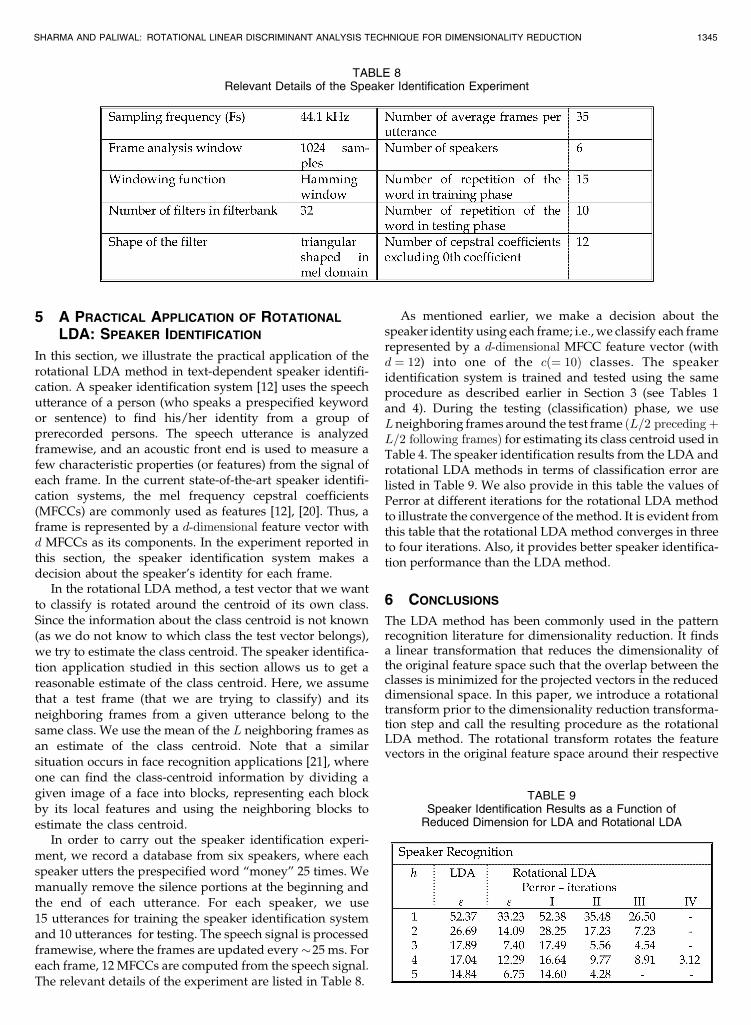
In order to carry out the speaker identification experi-ment, we record a database from six speakers, where eachspeaker utters the prespecified word “money” 25 times. Wemanually remove the silence portions at the beginning andthe end of each utterance. For each speaker, we use15 utterances for training the speaker identification systemand 10 utterances for testing. The speech signal is processedframewise, where the frames are updated every25 ms. Foreach frame, 12 MFCCs are computed from the speech signal.The relevant details of the experiment are listed in Table 8.

As mentioned earlier, we make a decision about thespeaker identity using each frame; i.e., we classify each framerepresented by a d-dimensional MFCC feature vector (withd ¼ 12) into one of the cð¼ 10Þ classes. The speakeridentification system is trained and tested using the sameprocedure as described earlier in Section 3 (see Tables 1and 4). During the testing (classification) phase, we useLneighboring frames around the test frame ðL=2 precedingþL=2 following framesÞ for estimating its class centroid used inTable 4. The speaker identification results from the LDA androtational LDA methods in terms of classification error arelisted in Table 9. We also provide in this table the values ofPerror at different iterations for the rotational LDA methodto illustrate the convergence of the method. It is evident fromthis table that the rotational LDA method converges in threeto four iterations. Also, it provides better speaker identifica-tion performance than the LDA method.

6 CONCLUSIONS

The LDA method has been commonly used in the patternrecognition literature for dimensionality reduction. It findsa linear transformation that reduces the dimensionality ofthe original feature space such that the overlap between theclasses is minimized for the projected vectors in the reduceddimensional space. In this paper, we introduce a rotationaltransform prior to the dimensionality reduction transforma-tion step and call the resulting procedure as the rotationalLDA method. The rotational transform rotates the featurevectors in the original feature space around their respective


TABLE 8Relevant Details of the Speaker Identification Experiment

TABLE 9Speaker Identification Results as a Function of

Reduced Dimension for LDA and Rotational LDA

class centroids. We have mathematically derived a proce-dure that finds the rotational transform, as well as thedimensionality-reduction transform, such that the overlapbetween the classes is minimized in the reduced featurespace. We have provided illustrative examples that demon-strate that the rotational LDA method is more effective inreducing this overlap between the classes than the LDAmethod. By introducing rotational transform in the originalfeature space, the rotational LDA method can be envisionedas a more generalized version of the LDA method.

We have conducted experiments on a number of publiclyavailable data corpuses to evaluate the pattern classificationperformance of the rotational LDA method. We have reportedresults that demonstrate that the rotational LDA methodoutperforms the LDA method on all the data corpuses.

APPENDIX

SOME COMPUTATIONAL ISSUES RELATED TO THE

TRAINING PHASE OF ROTATIONAL LDA

We have seen that the rotational LDA method is moreeffective in reducing the overlap between classes in thereduced-dimensional space than the conventional LDAmethod and hence results in better classification perfor-mance. However, this improvement in performance comeswith some additional computational cost during thetraining phase of the rotational LDA method. Some ofthese computational issues are listed as follows:

1. The rotational LDA algorithm (Table 1) computesthe basic (conventional) LDA at each stage ofiteration. This means that the algorithm is comput-ing the within-class scatter matrix ðSW Þ and thebetween class-scatter matrix ðSbÞ for each iteration.

2. It can also be observed in Table 1 that the trainingfeature vectors are updated at each iteration.

3. The use of an expectation operator in (11) (or step 9in Table 1) increases the computational cost.

We provide here some suggestions to address thesecomputational issues. For the first computational issue, theprocedure can be modified such that it will not compute SWand Sb for each step of the iteration process. We can modifythese matrices by investigating how SW and Sb alter duringthe iteration process. It is known that SW is the sum ofscatter matrices Mj [7], i.e.

SW ¼Xcj¼1

Mj;

where Mj ¼P

x2��jðx� ��xj

Þðx� ��xjÞT.

After rotation ��, feature vector x will change according to(16); this would change the scatter matrix as

Mj ¼ ��TXx 2 ��j

x� ��xj

� �x� ��xj

� �T

24

35�� ¼ ��TMj��:

Therefore, the modified within-class scatter matrix willbecome

SW ¼ ��TSW��:

On the other hand, Sb depends on the class centroids andthe total mean vector [7], which would not change duringthe rotation. Therefore, Sb will remain unchanged withrespect to rotation. Thus, the new value of orientation W

can be computed directly from rotation �� and the previousvalue of SW using eigenvalue decomposition; i.e.

SW ��TSW��;

Sbwi ¼ �iSSWwi;

where wi are the column vectors of W corresponding to �i.This would save processing time in computing thesematrices for each of the iterations. It should be noted herethat though we have used orientation W from the LDAtechnique, one could apply some other techniques insteadof LDA [22] together with the rotational method for theimprovement of recognition and/or classification. In thatcase, the optimization criteria will be different, dependingupon the technique then used.

The second computational issue can be addressed byintroducing some kind of weighting coefficients that wouldupdate the parameters depending upon the rotation andtheir previous values.

For the third computational issue, the expectationoperation can be omitted by introducing an online oradaptive version of the algorithm, where parameters maybe updated for every feature vector x instead of taking theclass average of feature vectors.

REFERENCES

[1] H. Anton, Calculus. John Wiley & Sons, 1995.[2] P.N. Belhumeur, J.P. Hespanha, and D.J. Kriegman, “Eigenfaces

versus Fisherfaces: Recognition Using Class Specific LinearProjection,” IEEE Trans. Pattern Analysis and Machine Intelligence,vol. 19, no. 7, pp. 711-720, July 1997.

[3] C.M. Bishop, Pattern Recognition and Machine Learning. Springer,2006.

[4] C.L. Blake and C.J. Merz, UCI Repository of Machine LearningDatabases, Dept. of Information and Computer Science, Univ. ofCalifornia, Irvine, http://www.ics.uci.edu/~mlearn, 1998.

[5] H. Cevikalp, M. Neamtu, M. Wlkes, and A. Barkana, “Dis-criminative Common Vectors for Face Recognition,” IEEE Trans.Pattern Analysis and Machine Intelligence, vol. 27, no. 1, pp. 4-13,Jan. 2005.

[6] L.-F. Chen, H.-Y.M. Liao, M.-T. Ko, J.-C. Lin, and G.-J. Yu, “A NewLDA-Based Face Recognition System Which Can Solve the SmallSample Size Problem,” Pattern Recognition, vol. 33, pp. 1713-1726,2000.

[7] R.O. Duda and P.E. Hart, Pattern Classification and Scene Analysis.John Wiley & Sons, 1973.

[8] J.H. Friedman, “Regularized Discriminant Analysis,” J. Am.Statistical Assoc., vol. 84, pp. 165-175, 1989.

[9] K. Fukunaga, Introduction to Statistical Pattern Recognition. Aca-demic Press, 1990.

[10] S.G. Garofalo, L.F. Lori, F.M. William, F.G. Jonathan, P.S. David,and D.L. Nancy, “The DARPA TIMIT Acoustic-Phonetic Con-tinuous Speech Corpus CDROM,” NIST, 1986.

[11] Y. Guo, T. Hastie, and R. Tinshirani, “Regularized DiscriminantAnalysis and Its Application in Microarrays,” Biostatistics, vol. 8,no. 1, pp. 86-100, 2007.

[12] X. Huang, A. Acero, and H.-W. Hon, Spoken Language Processing.Prentice Hall, 2001.

[13] A. Hyvarinen, “Fast and Robust Fixed-Point Algorithms forIndependent Component Analysis,” IEEE Trans. Neural Networks,vol. 10, no. 3, pp. 626-634, 1999.

[14] A. Hyvarinen and E. Oja, “A Fast Fixed-Point Algorithm forIndependent Component Analysis,” Neural Computation, vol. 9,no. 7, pp. 1483-1492, 1997.


[15] A.K. Jain, R.P.W. Duin, and J. Mao, “Statistical Pattern Recogni-tion: A Review,” IEEE Trans. Pattern Analysis and MachineIntelligence, vol. 22, no. 1, pp. 4-37, Jan. 2000.

[16] W.J. Krzanowski, P. Jonathan, W.V. McCarthy, and M.R. Thomas,“Discriminant Analysis with Singular Covariance Matrices:Methods and Applications to Spectroscopic Data,” AppliedStatistics, vol. 44, pp. 101-115, 1995.

[17] R. Lotlikar and R. Kothari, “Fractional-Step DimensionalityReduction,” IEEE Trans. Pattern Analysis and Machine Intelligence,vol. 22, no. 6, pp. 623-627, June 2000.

[18] J. Lu, K.N. Plataniotis, and A.N. Venetsanopoulos, “FaceRecognition Using LDA-Based Algorithms,” IEEE Trans. NeuralNetworks, vol. 14, no. 1, pp. 195-200, 2003.

[19] S. Raudys and R.P.W. Duin, “On Expected Classification Error ofthe Fisher Linear Classifier with Pseudo-Inverse CovarianceMatrix,” Pattern Recognition Letters, vol. 19, nos. 5-6, pp. 385-392,1998.

[20] D.A. Reynolds, T.F. Quatieri, and R.B. Dunn, “Speaker Verifica-tion Using Adapted Gaussian Mixture Models,” Digital SignalProcessing, vol. 10, no. 1-3, pp. 19-41, 2000.

[21] C. Sanderson and K.K. Paliwal, “Identity Verification UsingSpeech and Face Information,” Digital Signal Processing, vol. 14,no. 5, pp. 449-480, 2004.

[22] A. Sharma, K.K. Paliwal, and G.C. Onwubolu, “Class-DependentPCA, LDA and MDC: A Combined Classifier for PatternClassification,” Pattern Recognition, vol. 39, no. 7, pp. 1215-1229,2006.

[23] A. Sharma and K.K. Paliwal, “A Gradient Linear DiscriminantAnalysis for Small Sample Sized Problem,” Neural ProcessingLetters, vol. 27, no. 1, pp. 17-24, 2008.

[24] D.L. Swets and J. Weng, “Using Discriminative Eigenfeatures forImage Retrieval,” IEEE Trans. Pattern Analysis and MachineIntelligence, vol. 18, no. 8, pp. 831-836, Aug. 1996.

[25] Q. Tian, M. Barbero, Z.H. Gu, and S.H. Lee, “Image Classificationby the Foley-Sammon Transform,” Optical Eng., vol. 25, no. 7,pp. 834-840, 1986.

[26] S. Young, G. Evermann, T. Hain, D. Kershaw, G. Moore, J. Odell,D. Ollason, D. Povey, V. Valtchev, and P. Woodland, The HTKBook Version 3.2. Cambridge Univ., 2002.

[27] J. Ye, “Characterization of a Family of Algorithms for GeneralizedDiscriminant Analysis on Undersampled Problems,” J. MachineLearning Research, vol. 6, pp. 483-502, 2005.

[28] H. Yu and J. Yang, “A Direct LDA Algorithm for High-Dimensional Data—With Application to Face Recognition,”Pattern Recognition, vol. 34, pp. 2067-2070, 2001.

Alok Sharma received the BTech degree fromthe University of the South Pacific (USP), Suva,Fiji, in 2000 and the MEng degree, with anacademic excellence award, and the PhDdegree in the area of pattern recognition fromGriffith University, Brisbane, Australia, in 2001and 2006, respectively. He is currently servingas an academic and the head of the Division ofElectrical/Electronics, School of Engineeringand Physics, USP. He is also with the Signal

Processing Laboratory, Griffith University. He participated in variousprojects carried out in conjunction with Motorola (Sydney), Auslog Pty.Ltd. (Brisbane), CRC Micro Technology (Brisbane), and the FrenchEmbassy (Suva). He also received several grant packages. Some ofthem are from the French Embassy, the University Research Commit-tee, Fiji, and the SPAS Research Committee, Fiji. His research interestsinclude pattern recognition, computer security, and human cancerclassification. He reviewed several articles from journals like IEEETransactions on Neural Networks, IEEE Transaction on Systems, Man,and Cybernetics, Part A: Systems and Humans, IEEE Journal onSelected Topics in Signal Processing, IEEE Transactions on Knowledgeand Data Engineering, Computers & Security, and Pattern Recognition.He is a member of the IEEE.

Kuldip K. Paliwal received the BS degree fromAgra University, Agra, India, in 1969, theMS degree from Aligarh Muslim University,Aligarh, India, in 1971, and the PhD degreefrom Bombay University, Bombay, India, in1978. He has been carrying out research in thearea of speech processing since 1972. He hasworked at a number of organizations includingthe Tata Institute of Fundamental Research,Bombay, India, the Norwegian Institute of

Technology, Trondheim, Norway, the University of Keele, UnitedKingdom, AT&T Bell Laboratories, Murray Hill, New Jersey, AT&TShannon Laboratories, Florham Park, New Jersey, and AdvancedTelecommunication Research Laboratories, Kyoto. Since July 1993, hehas been a professor in the School of Microelectronic Engineering,Griffith University, Brisbane, Australia. His current research interestsinclude speech recognition, speech coding, speaker recognition, speechenhancement, face recognition, image coding, pattern recognition, andartificial neural networks. He has published more than 250 papers inthese research areas. He has coedited two books: Speech Coding andSynthesis (published by Elsevier) and Speech and Speaker Recogni-tion: Advanced Topics (published by Kluwer Academic Publishers). Hewas an associate editor of the IEEE Transactions on Speech and AudioProcessing during the periods 1994-1997 and 2003-2004. He alsoserved as an associate editor of the IEEE Signal Processing Lettersfrom 1997 to 2000. He is currently serving the journal SpeechCommunication (published by Elsevier) as its editor in chief. He hasserved in the IEEE Signal Processing Society’s Neural NetworksTechnical Committee as a founding member from 1991 to 1995 andthe Speech Processing Technical Committee from 1999 to 2003. Hewas the general cochair of the 10th IEEE Workshop on Neural Networksfor Signal Processing (NNSP ’00). He received the IEEE SignalProcessing Society’s Best (Senior) Paper Award in 1995 for his paperon LPC quantization. He is a Fellow of the Acoustical Society of Indiaand a member of the IEEE.

. For more information on this or any other computing topic,please visit our Digital Library at www.computer.org/publications/dlib.


Documents

1336 IEEE TRANSACTIONS ON KNOWLEDGE AND … Linear Discriminant Analysis Technique for Dimensionality Reduction Alok Sharma, Member, IEEE, and Kuldip K. Paliwal,Member, IEEE Abstract—The