Embed Size (px)
DESCRIPTION
Modeling of Induction Motors using DQ analysis
Citation preview
Topic 4: Modeling of Induction Motor using qd0 Transformations
Spring 2004
ECE 8830 - Electric Drives
Introduction
Steady state model developed in previous topic neglects electrical transients due to load changes and stator frequency variations. Such variations arise in applications involving variable-speed drives.
Variable-speed drives are converter-fed from finite sources, which unlike the utility supply, are limited by switch ratings and filter sizes, i.e. they cannot supply large transient power.
Introduction (cont’d)
Thus, we need to evaluate dynamics of converter-fed variable-speed drives to assess the adequacy of the converter switches and the converters for a given motor and their interaction to determine the excursions of currents and torque in the converter and motor. Thus, the dynamic model considers the instantaneous effects of varying voltages/currents, stator frequency and torque disturbance.
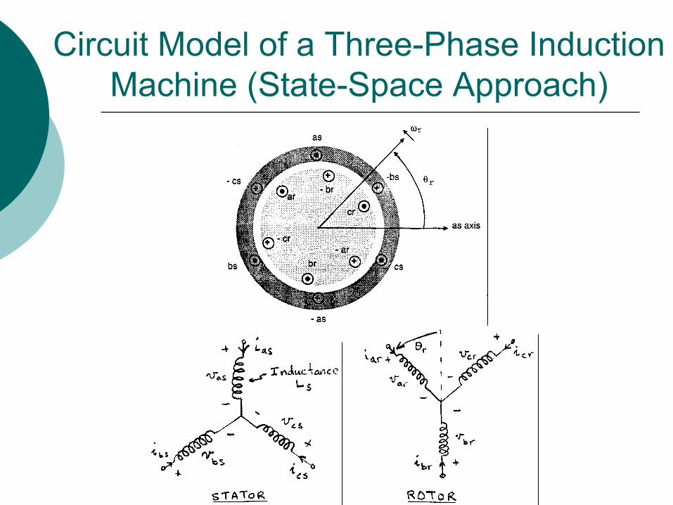
Circuit Model of a Three-Phase Induction Machine (State-Space Approach)
Voltage Equations
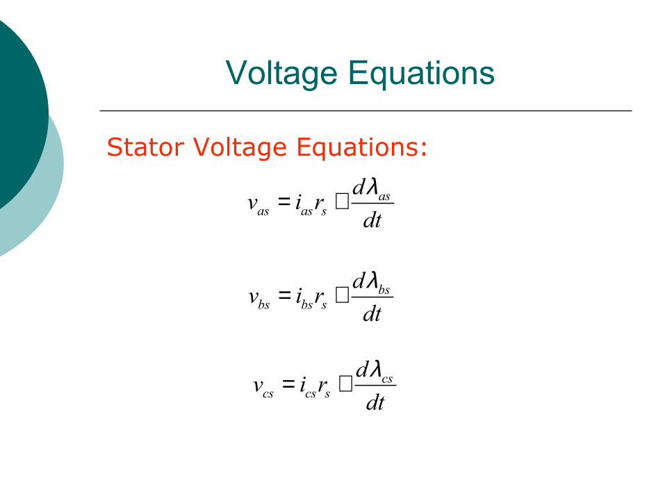
Stator Voltage Equations:
asas as s
dv i r
dt
λ= +
bsbs bs s
dv i r
dt
λ= +
cscs cs s
dv i r
dt
λ= +
Voltage Equations (cont’d)
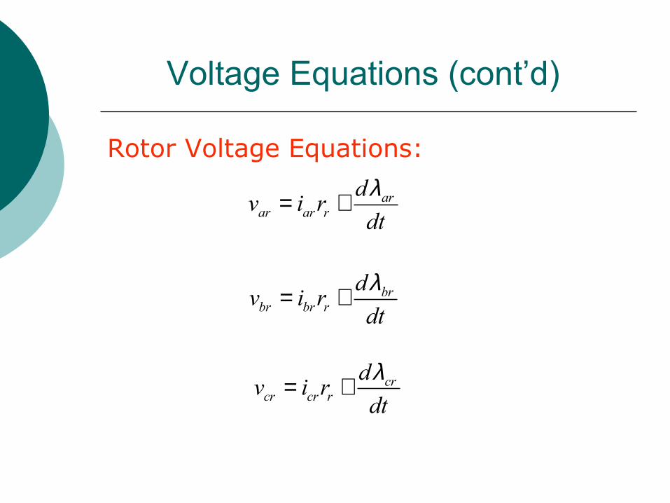
Rotor Voltage Equations:
arar ar r
dv i r
dt
λ= +
brbr br r
dv i r
dt
λ= +
crcr cr r
dv i r
dt
λ= +
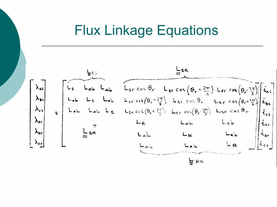
Flux Linkage Equations
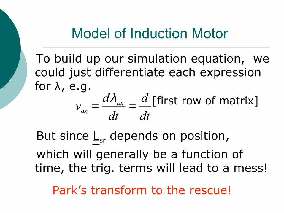
Model of Induction Motor
To build up our simulation equation, we could just differentiate each expression for λ, e.g.
But since Lsr depends on position,
which will generally be a function of time, the trig. terms will lead to a mess!
Park’s transform to the rescue!
asas
d dv
dt dt
λ= = [first row of matrix]
Park’s Transformation
The Park’s transformation is a three-phase to two-phase transformation for synchronous machine analysis. It is used to transform the stator variables of a synchronous machine onto a dq reference frame that is fixed to the rotor.
The +ve q-axis is aligned with the magnetic axis of the field winding and the +ve d-axis is defined as leading the +ve q-axis by π/2. (see Fig. 5.16c Ong on next slide).
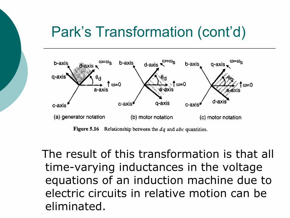
Park’s Transformation (cont’d)
The result of this transformation is that all
time-varying inductances in the voltage equations of an induction machine due to electric circuits in relative motion can be eliminated.
Park’s Transformation (cont’d)
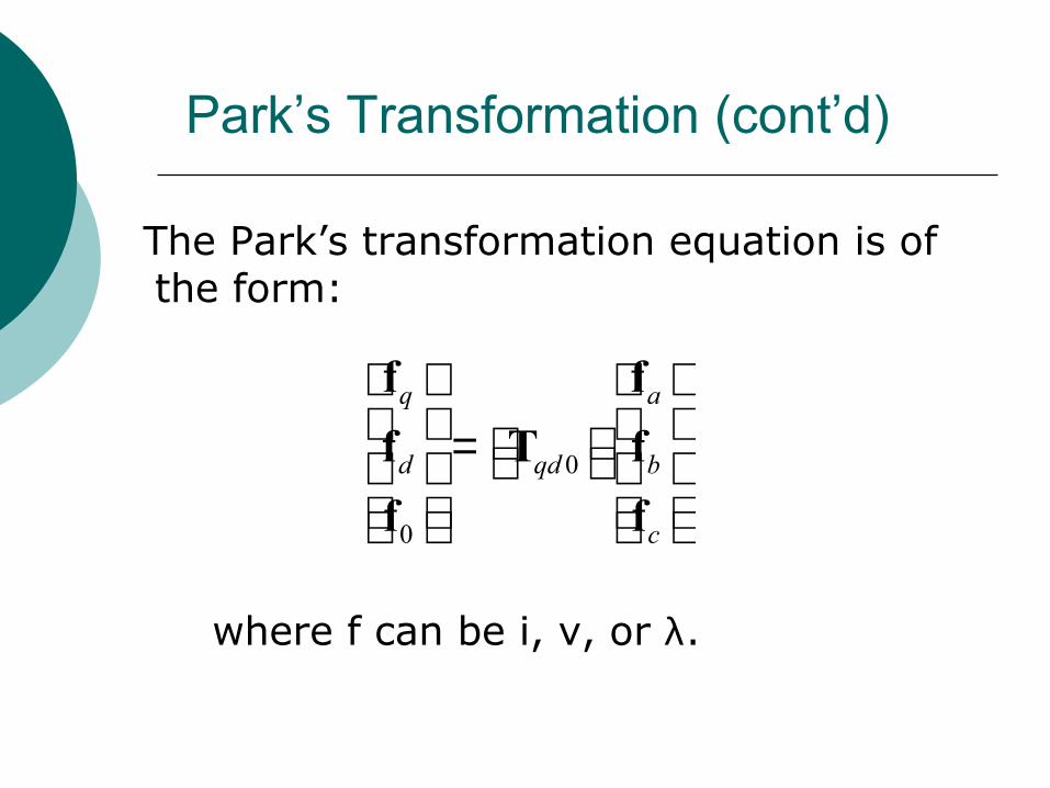
The Park’s transformation equation is of the form:
where f can be i, v, or λ.
0
0
q a
d qd b
c
=
f f
f T f
f f
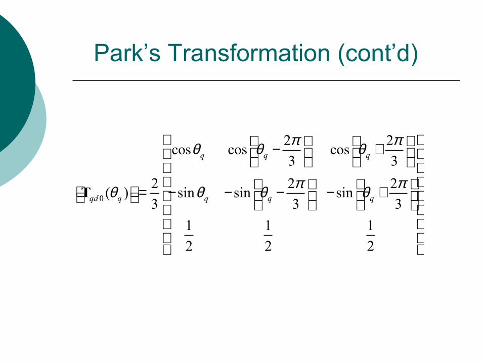
Park’s Transformation (cont’d)
0
2 2cos cos cos
3 3
2 2 2( ) sin sin sin
3 3 3
1 1 1
2 2 2
q q q
qd q q q q
π πθ θ θ
π πθ θ θ θ
− + = − − − − +
T
Park’s Transformation (cont’d)
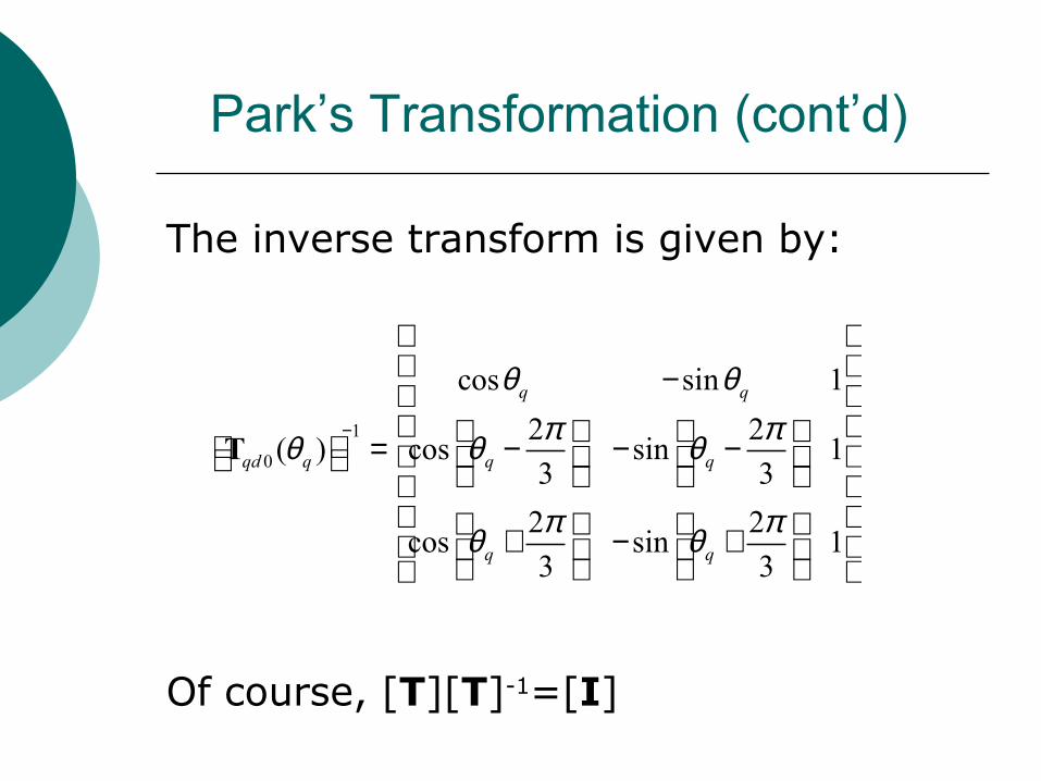
The inverse transform is given by:
Of course, [T][T]-1=[I]
1
0
cos sin 1
2 2( ) cos sin 1
3 3
2 2cos sin 1
3 3
q q
qd q q q
q q
θ θπ πθ θ θ
π πθ θ
−
− = − − − + − +
T
Park’s Transformation (cont’d)
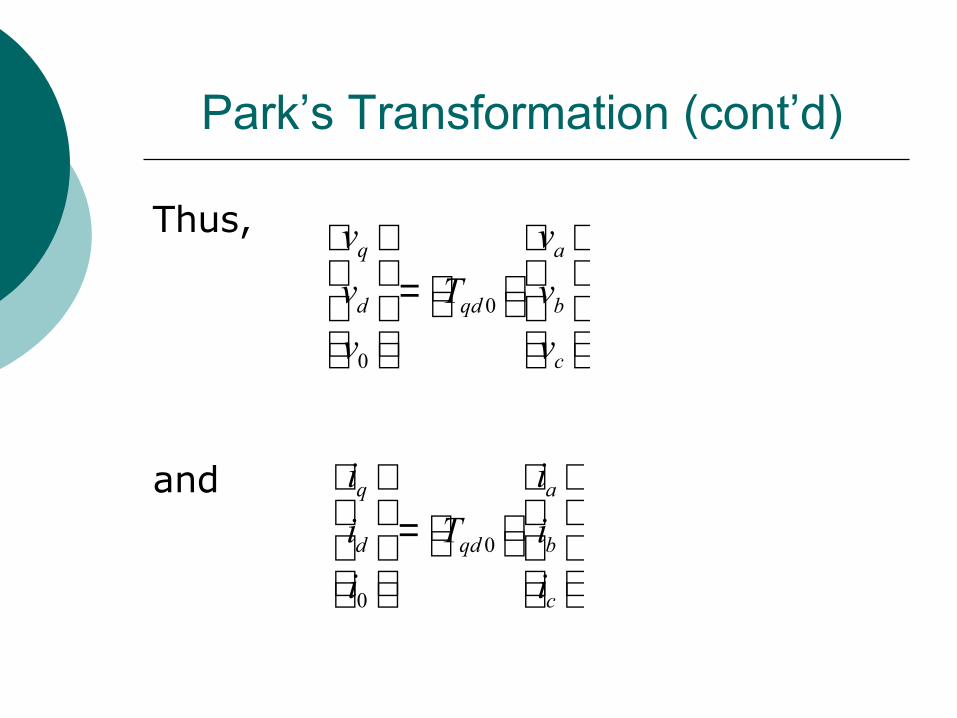
Thus,
and
0
0
q a
d qd b
c
v v
v T v
v v
=
0
0
q a
d qd b
c
i i
i T i
i i
=
Induction Motor Model in qd0
Acknowledgement:
The following notes covering the induction motor modeling in qd0 space are mostly courtesy of Dr. Steven Leeb of MIT.
Induction Motor Model in qd0 (cont’d)
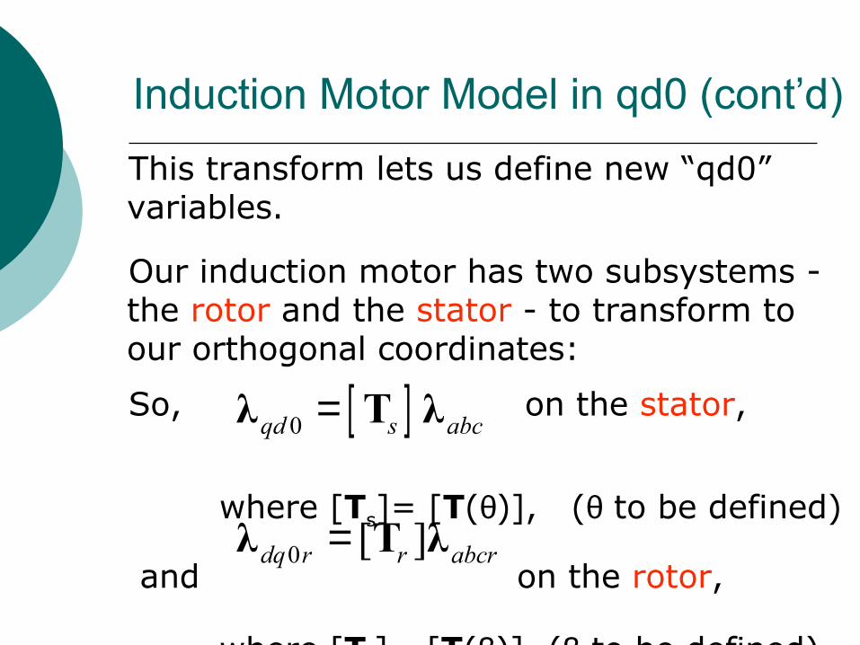
This transform lets us define new “qd0” variables.
Our induction motor has two subsystems - the rotor and the stator - to transform to our orthogonal coordinates:
So, on the stator,
where [Ts]= [T(θ)], (θ to be defined)
and on the rotor,
where [Tr]= [T(β)], (β to be defined)
[ ]0qd s abc=λ T λ
0 [ ]dq r r abcr=λ T λ
Induction Motor Model in qd0 (cont’d)
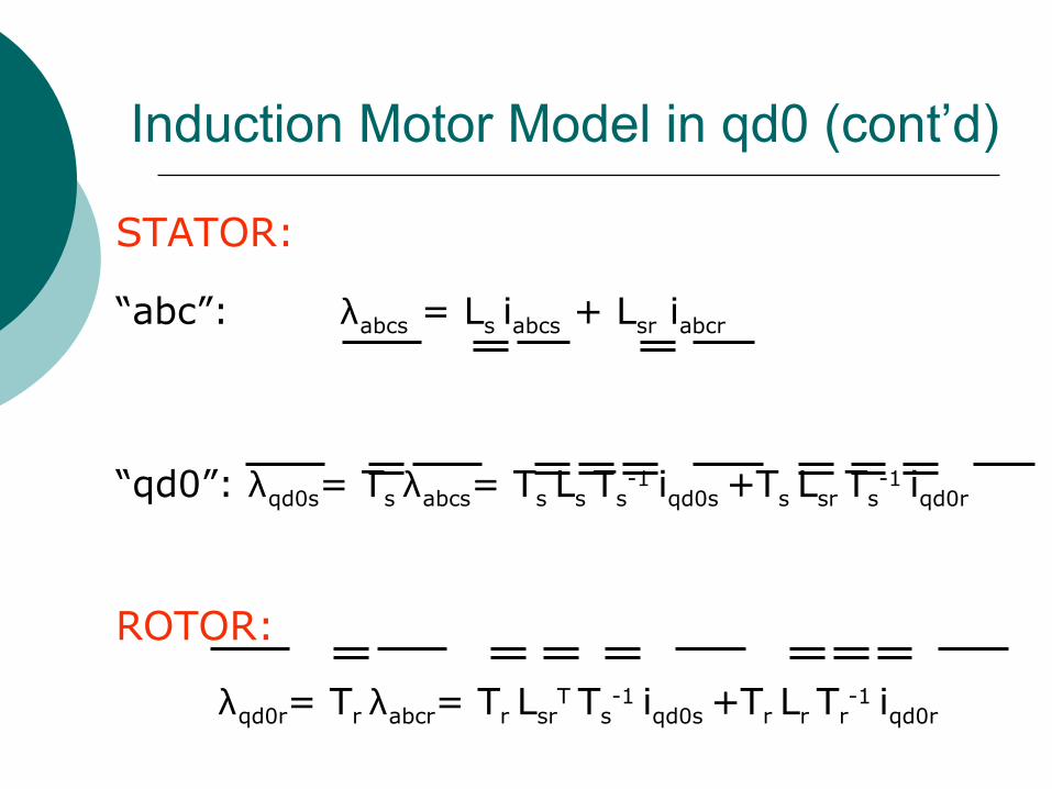
STATOR:
“abc”: λabcs = Ls iabcs + Lsr iabcr
“qd0”: λqd0s= Ts λabcs= Ts Ls Ts-1 iqd0s +Ts Lsr Ts
-1 iqd0r
ROTOR:
λqd0r= Tr λabcr= Tr LsrT Ts
-1 iqd0s +Tr Lr Tr-1 iqd0r
Induction Motor Model in qd0 (cont’d)
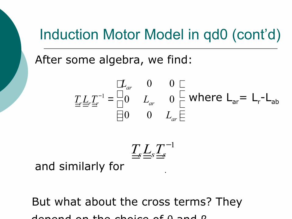
After some algebra, we find:
where Lar= Lr-Lab
and similarly for .
But what about the cross terms? They
depend on the choice of θ and β. Let β = θ - θr , where θr is the rotor position.
1
0 0
0 0
0 0
ar
r r r ar
ar
L
T L T L
L
−
=
1s s sT L T −
Induction Motor Model in qd0 (cont’d)
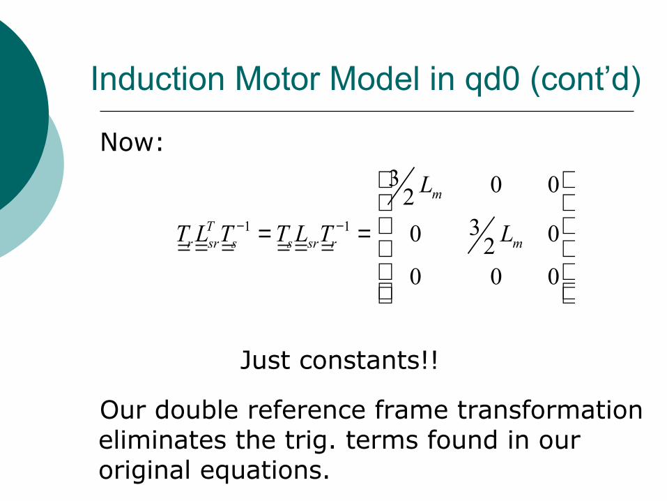
Now:
Just constants!!
Our double reference frame transformation eliminates the trig. terms found in our original equations.
1 1
3 0 0230 02
0 0 0
m
Tr sr s s sr r m
L
T L T T L T L− −
= =
Induction Motor Model in qd0 (cont’d)
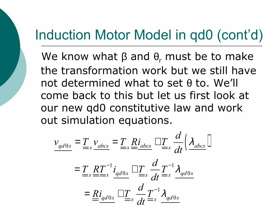
We know what β and θr must be to make the transformation work but we still have not determined what to set θ to. We’ll come back to this but let us first look at our new qd0 constitutive law and work out simulation equations.
( )0qd s abcs abcs abcss s s
dv T v T Ri T
dtλ= = +
1 10 0qd s qd ss s s s
dT RT i T T
dtλ− −= +
10 0qd s qd ss s
dRi T T
dtλ−= +
Induction Motor Model in qd0 (cont’d)
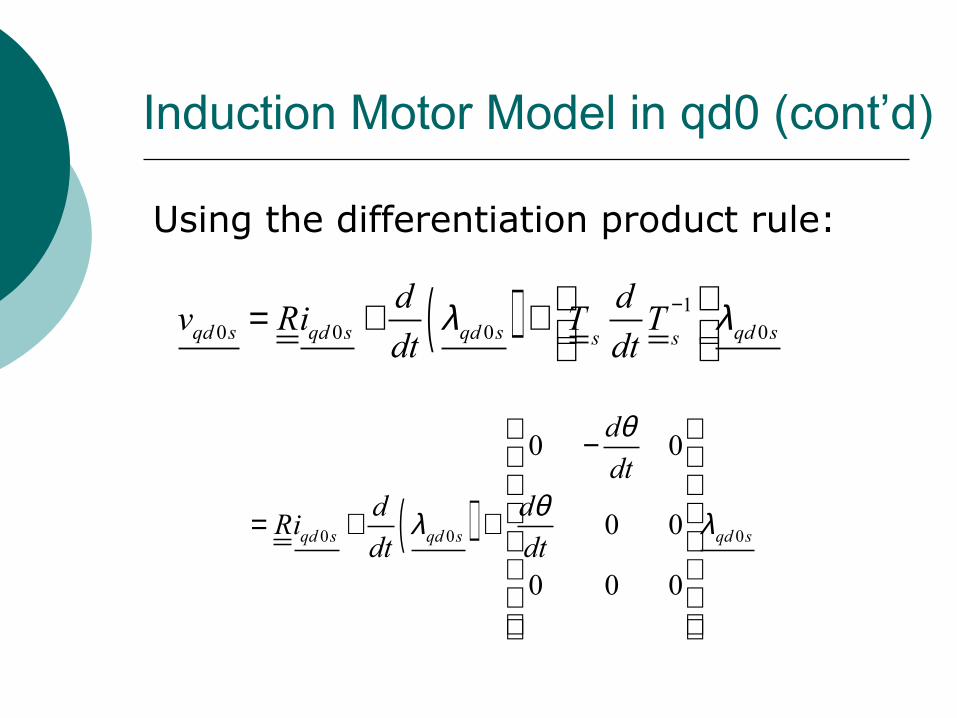
Using the differentiation product rule:
( ) 10 0 0 0qd s qd s qd s qd ss s
d dv Ri T T
dt dtλ λ− = + +
( )0 0 0
0 0
0 0
0 0 0
qd s qd s qd s
d
dtd d
Ridt dt
θ
θλ λ
− = + +
Induction Motor Model in qd0 (cont’d)
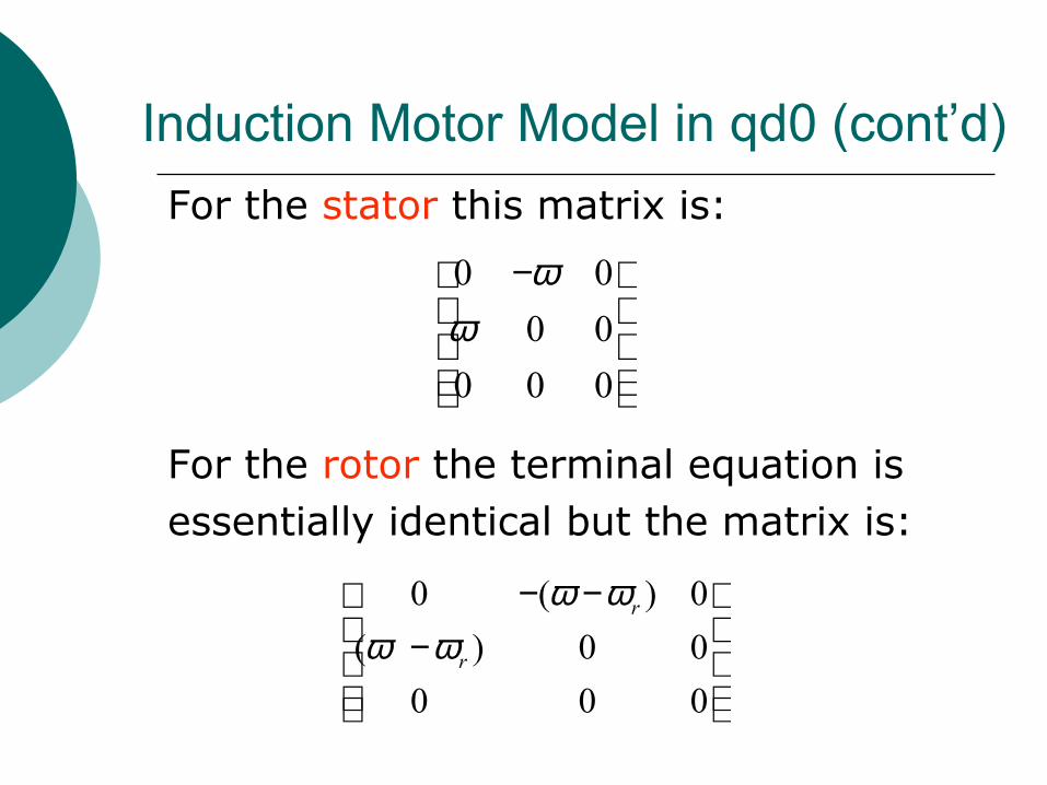
For the stator this matrix is:
For the rotor the terminal equation is essentially identical but the matrix is:
0 0
0 0
0 0 0
ωω
−
0 ( ) 0
( ) 0 0
0 0 0
r
r
ω ωω ω
− − −
Induction Motor Model in qd0 (cont’d)
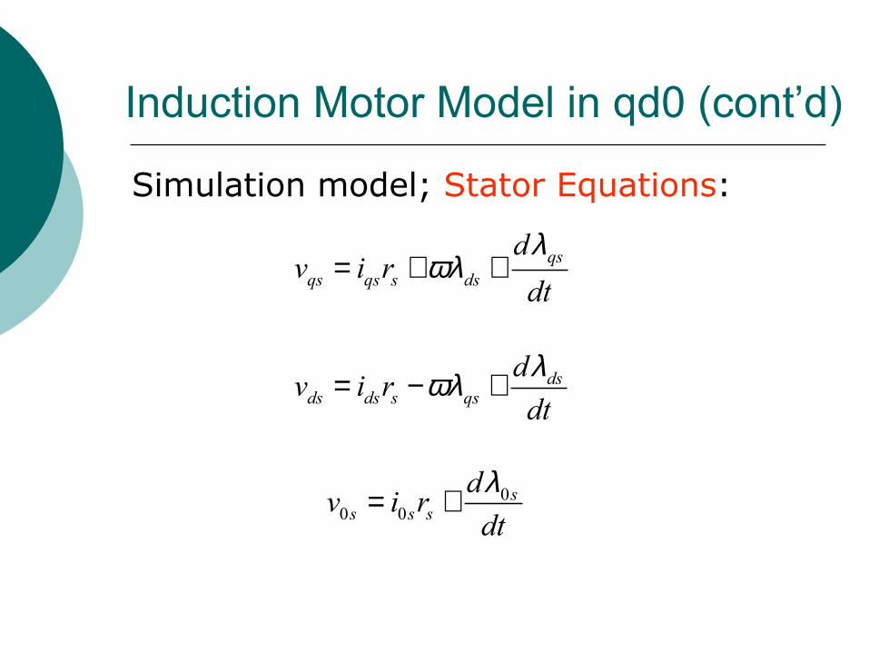
Simulation model; Stator Equations:
dsds ds s qs
dv i r
dt
λωλ= − +
qsqs qs s ds
dv i r
dt
λωλ= + +
00 0
ss s s
dv i r
dt
λ= +
Induction Motor Model in qd0 (cont’d)
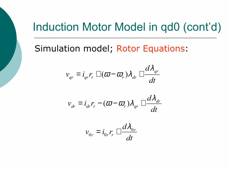
Simulation model; Rotor Equations:
( ) drdr dr r r qr
dv i r
dt
λω ω λ= − − +
( ) qrqr qr r r dr
dv i r
dt
λω ω λ= + − +
00 0
rr r r
dv i r
dt
λ= +
Induction Motor Model in qd0 (cont’d)
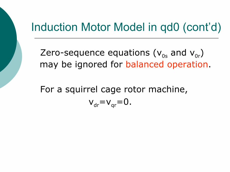
Zero-sequence equations (v0s and v0r) may be ignored for balanced operation.
For a squirrel cage rotor machine, vdr=vqr=0.
Induction Motor Model in qd0 (cont’d)
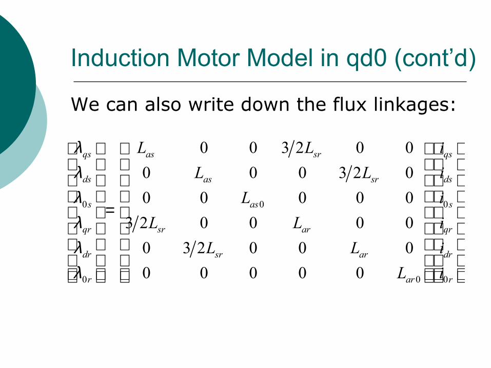
We can also write down the flux linkages:
0 0 0
0 0 0
0 0 3 2 0 0
0 0 0 3 2 0
0 0 0 0 0
3 2 0 0 0 0
0 3 2 0 0 0
0 0 0 0 0
qs as sr qs
ds as sr ds
s as s
qr sr ar qr
dr sr ar dr
r ar r
L L i
L L i
L i
L L i
L L i
L i
λλλλλλ
=
Induction Motor Model in qd0 (cont’d)
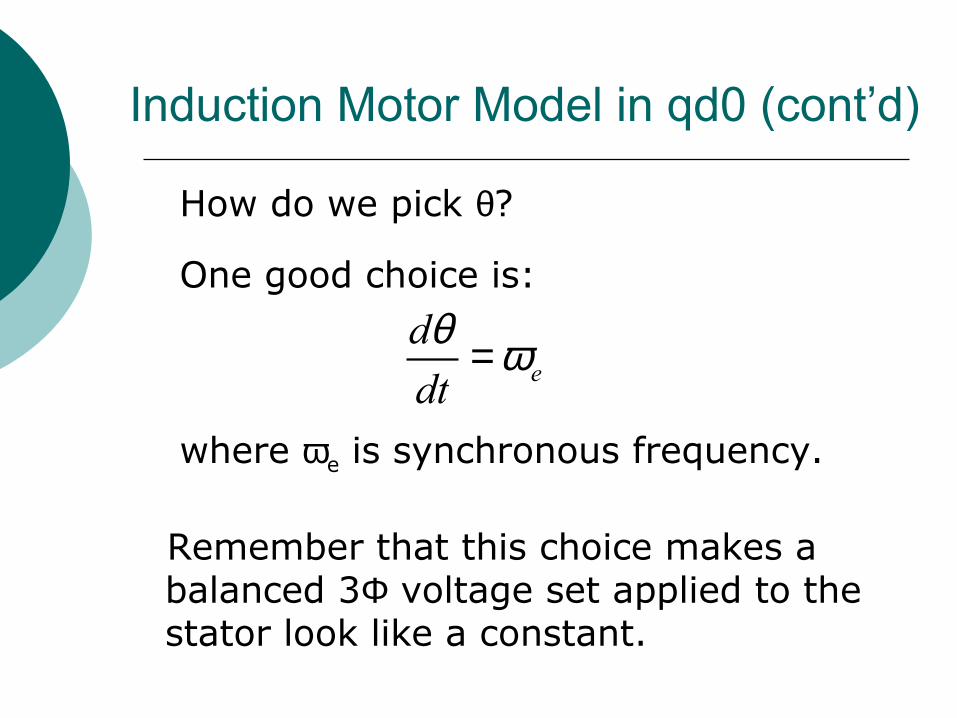
How do we pick θ?
One good choice is:
where ωe is synchronous frequency.
Remember that this choice makes a balanced 3Φ voltage set applied to the stator look like a constant.
e
d
dt
θ ω=
Induction Motor Model in qd0 (cont’d)
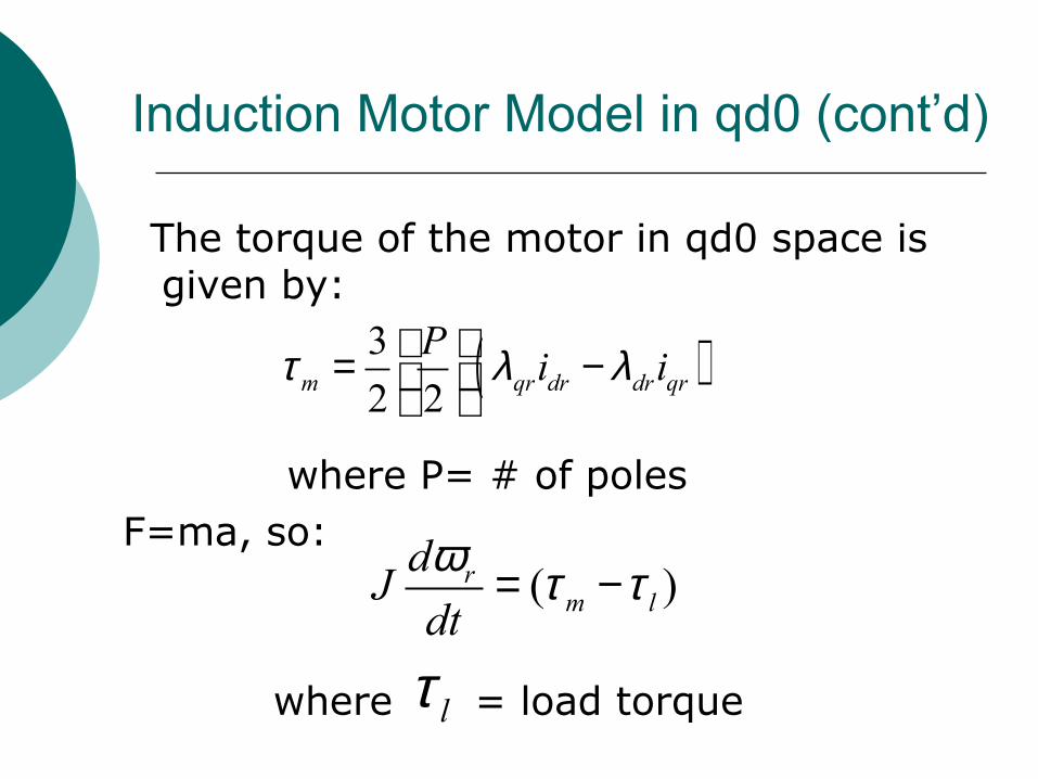
The torque of the motor in qd0 space is given by:
where P= # of polesF=ma, so:
where = load torque
( )3
2 2m qr dr dr qr
Pi iτ λ λ = −
( )rm l
dJdt
ω τ τ= −
lτ
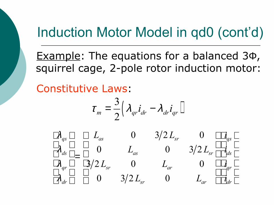
Example: The equations for a balanced 3Φ, squirrel cage, 2-pole rotor induction motor:
Constitutive Laws:
Induction Motor Model in qd0 (cont’d)
( )3
2m qr dr dr qri iτ λ λ= −
0 3 2 0
0 0 3 2
3 2 0 0
0 3 2 0
qs as sr qs
ds as sr ds
qr sr ar qr
dr sr ar dr
L L i
L L i
L L i
L L i
λλλλ
=
Induction Motor Model in qd0 (cont’d)
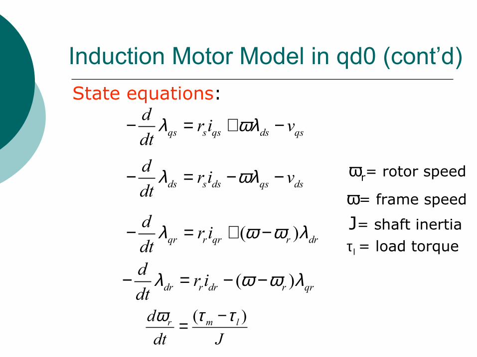
State equations:
ωr= rotor speed
ω= frame speed
J= shaft inertia τl = load torque
ds s ds qs ds
dr i v
dtλ ωλ− = − −
qs s qs ds qs
dr i v
dtλ ωλ− = + −
( )dr r dr r qr
dr i
dtλ ω ω λ− = − −
( )qr r qr r dr
dr i
dtλ ω ω λ− = + −
( )m lrd
dt J
τ τω −=
qd0 Induction Motor Model in Stationary Reference Frame
The qd0 induction motor model in the stationary reference frame can be obtained by setting ω=0. This model is known as the Stanley model and the equivalent circuits are given on the next slide.
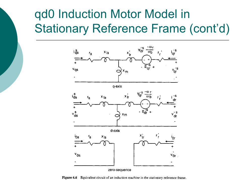
qd0 Induction Motor Model in Stationary Reference Frame (cont’d)
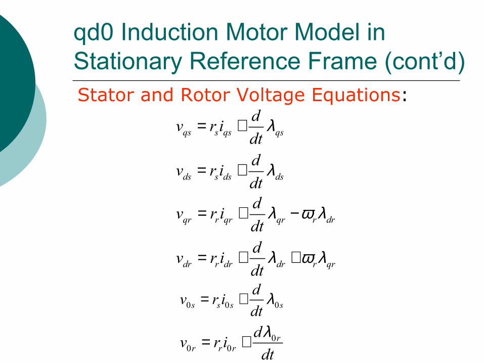
qd0 Induction Motor Model in Stationary Reference Frame (cont’d)Stator and Rotor Voltage Equations:
qs s qs qs
dv r i
dtλ= +
ds s ds ds
dv r i
dtλ= +
qr r qr qr r dr
dv r i
dtλ ω λ= + −
dr r dr dr r qr
dv r i
dtλ ω λ= + +
0 0 0s s s s
dv r i
dtλ= +
00 0
rr r r
dv r i
dt
λ= +
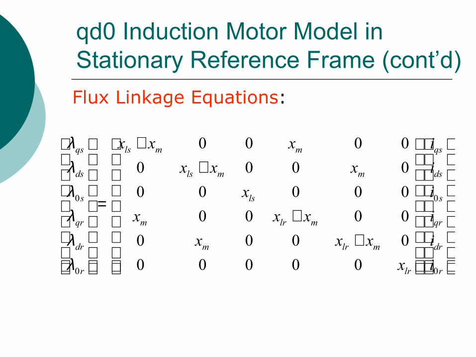
qd0 Induction Motor Model in Stationary Reference Frame (cont’d)
Flux Linkage Equations:
0 0
0 0
0 0 0 0
0 0 0 0
0 0 0 0 0
0 0 0 0
0 0 0 0
0 0 0 0 0
qs ls m m qs
ds ls m m ds
s ls s
qr m lr m qr
dr m lr m dr
r lr r
x x x i
x x x i
x i
x x x i
x x x i
x i
λλλλλλ
+ +
= + +
qd0 Induction Motor Model in Stationary Reference Frame (cont’d)
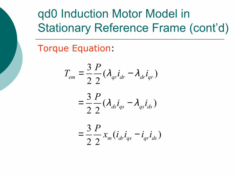
Torque Equation:
3( )
2 2em qr dr dr qr
PT i iλ λ= −
3( )
2 2 ds qs qs ds
Pi iλ λ= −
3( )
2 2 m dr qs qr ds
Px i i i i= −
Example 5.3 Krishnan
Induction Motor Model in qd0 Example
qd0 Induction Motor Model in Synchronous Reference Frame
The qd0 induction motor model in the synchronous reference frame can be obtained by setting ω= ωe . This model is known as the Kron model and the equivalent circuits are given on the next slide.
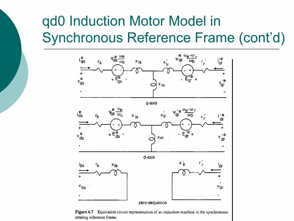
qd0 Induction Motor Model in Synchronous Reference Frame (cont’d)
qd0 Induction Motor Model in Synchronous Reference Frame (cont’d)
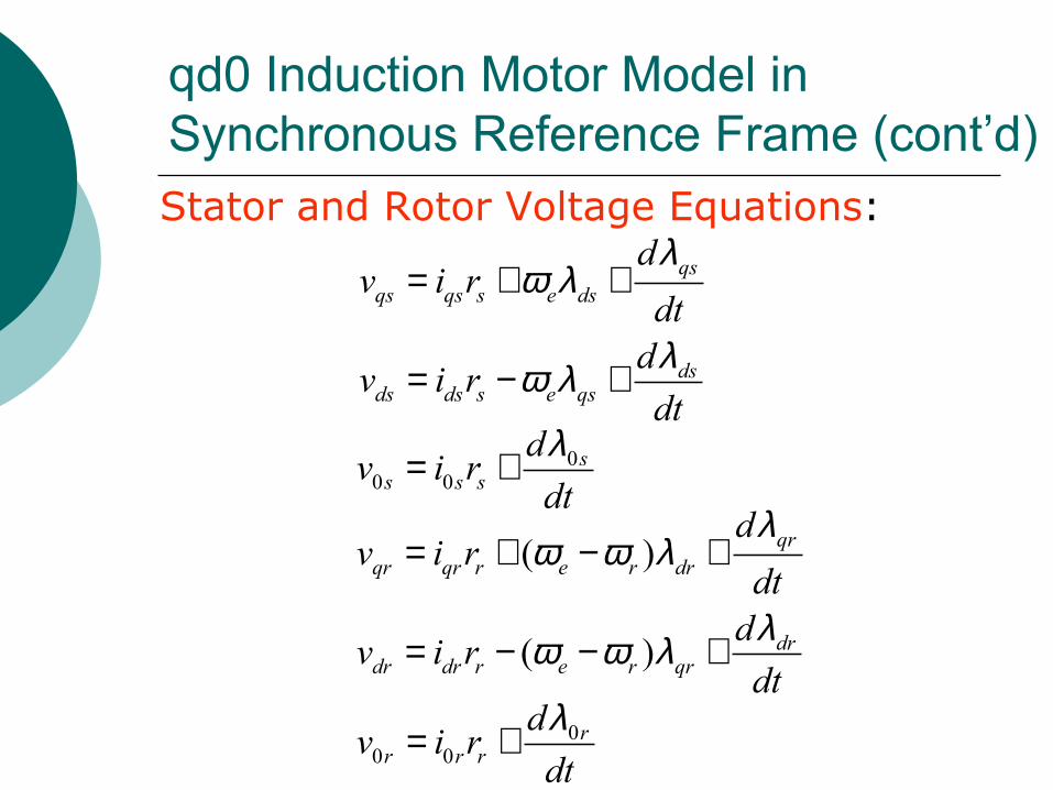
Stator and Rotor Voltage Equations:qs
qs qs s e ds
dv i r
dt
λω λ= + +
dsds ds s e qs
dv i r
dt
λω λ= − +
00 0
ss s s
dv i r
dt
λ= +
( ) drdr dr r e r qr
dv i r
dt
λω ω λ= − − +
( ) qrqr qr r e r dr
dv i r
dt
λω ω λ= + − +
00 0
rr r r
dv i r
dt
λ= +
qd0 Induction Motor Model in Synchronous Reference Frame (cont’d)
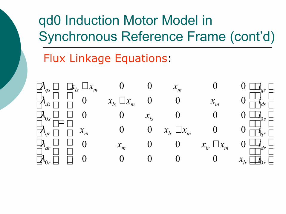
Flux Linkage Equations:
0 0
0 0
0 0 0 0
0 0 0 0
0 0 0 0 0
0 0 0 0
0 0 0 0
0 0 0 0 0
qs ls m m qs
ds ls m m ds
s ls s
qr m lr m qr
dr m lr m dr
r lr r
x x x i
x x x i
x i
x x x i
x x x i
x i
λλλλλλ
+ +
= + +
qd0 Induction Motor Model in Synchronous Reference Frame (cont’d)
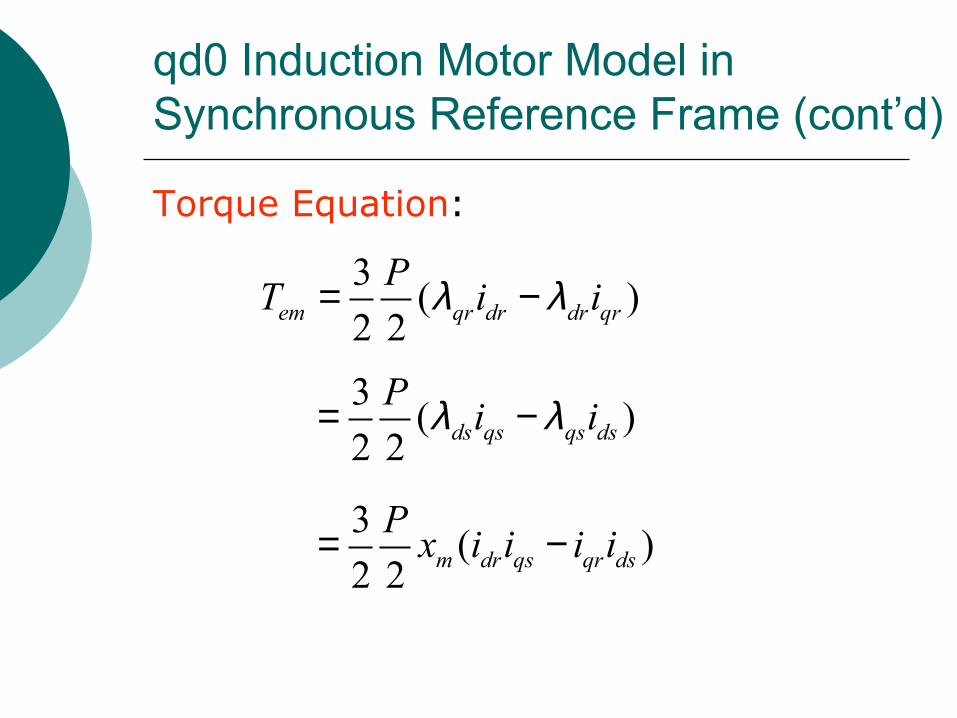
Torque Equation:
3( )
2 2em qr dr dr qr
PT i iλ λ= −
3( )
2 2 ds qs qs ds
Pi iλ λ= −
3( )
2 2 m dr qs qr ds
Px i i i i= −
Induction Motor Model in Synchronous Reference Frame Example
Example 5.5 Krishnan
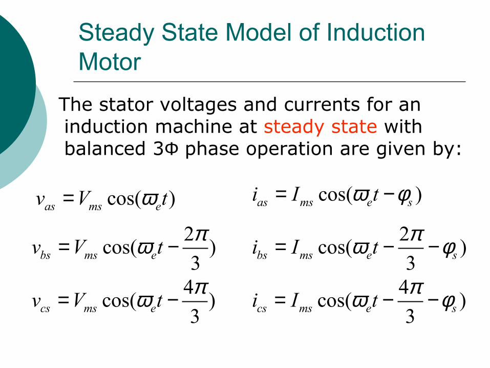
Steady State Model of Induction Motor
The stator voltages and currents for an induction machine at steady state with balanced 3Φ phase operation are given by:
cos( )as ms ev V tω=
2cos( )
3bs ms ev V tπω= −
4cos( )
3cs ms ev V tπω= −
cos( )as ms e si I tω φ= −
2cos( )
3bs ms e si I tπω φ= − −
4cos( )
3cs ms e si I tπω φ= − −
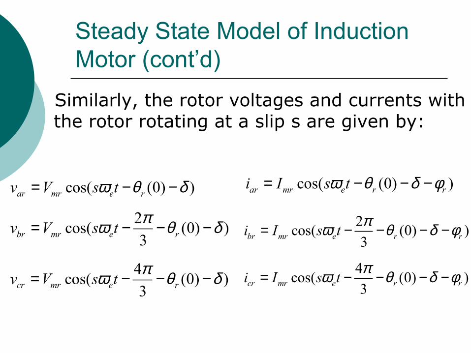
Steady State Model of Induction Motor (cont’d)
Similarly, the rotor voltages and currents with the rotor rotating at a slip s are given by:
cos( (0) )ar mr e rv V s tω θ δ= − − cos( (0) )ar mr e r ri I s tω θ δ φ= − − −
2cos( (0) )
3br mr e rv V s tπω θ δ= − − −
4cos( (0) )
3cr mr e rv V s tπω θ δ= − − −
2cos( (0) )
3br mr e r ri I s tπω θ δ φ= − − − −
4cos( (0) )
3cr mr e r ri I s tπω θ δ φ= − − − −
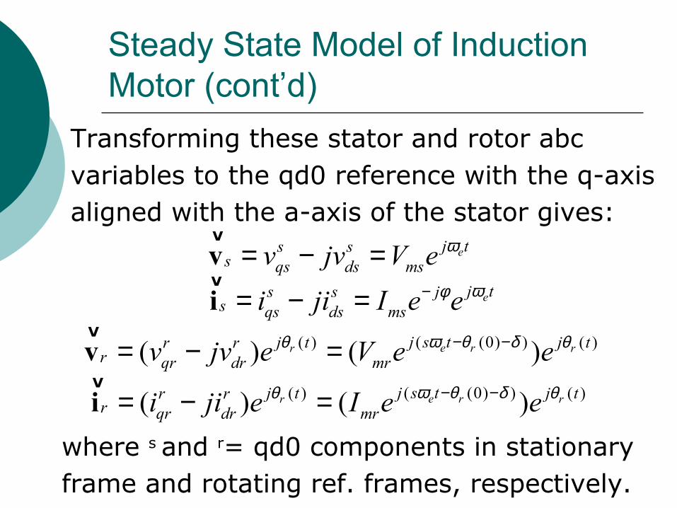
Steady State Model of Induction Motor (cont’d)
Transforming these stator and rotor abc variables to the qd0 reference with the q-axis aligned with the a-axis of the stator gives:
where s and r= qd0 components in stationary frame and rotating ref. frames, respectively.
ej ts ss qs ds msv jv V e ω= − =vv
ej ts s js qs ds msi ji I e e ωφ−= − =iv
( (0) )( ) ( )( ) ( )e rr rj s tj t j tr rr qr dr mrv jv e V e eω θ δθ θ− −= − =vv
( (0) )( ) ( )( ) ( )e rr rj s tj t j tr rr qr dr mri ji e I e eω θ δθ θ− −= − =iv
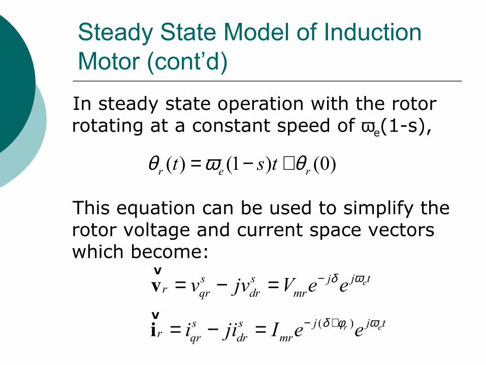
Steady State Model of Induction Motor (cont’d)
In steady state operation with the rotor rotating at a constant speed of ωe(1-s),
This equation can be used to simplify the rotor voltage and current space vectors which become:
( ) (1 ) (0)r e rt s tθ ω θ= − +
ej ts s jr qr dr mrv jv V e e ωδ−= − =vv
( ) er j tjs sr qr dr mri ji I e e ωδ φ− += − =iv
Steady State Model of Induction Motor (cont’d)
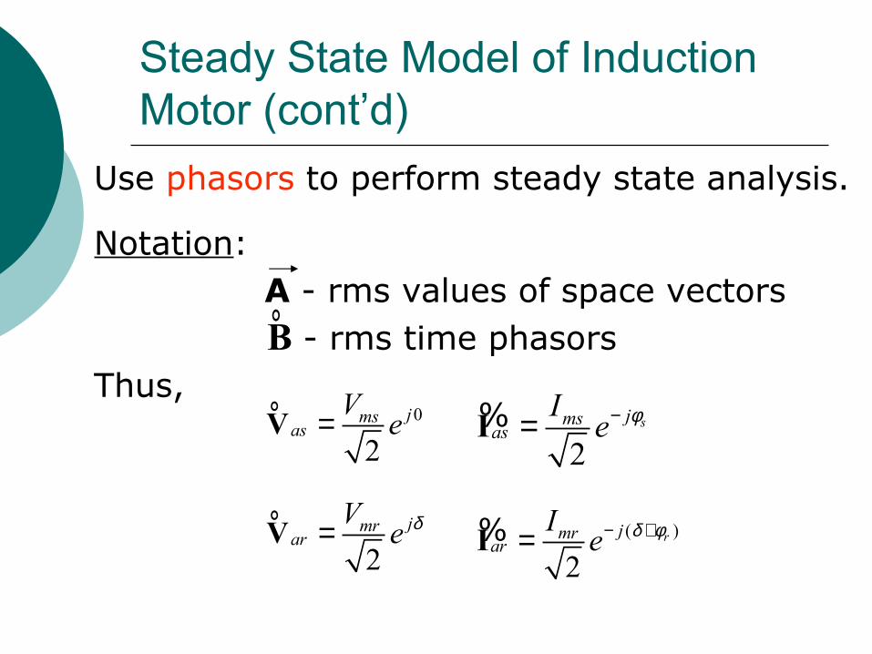
Use phasors to perform steady state analysis.
Notation: A - rms values of space vectors
- rms time phasors Thus,
°B
° 0
2jms
asVe=V
2sjms
asIe φ−=I%
°2
jmrar
Ve δ=V ( )
2rjmr
arIe δ φ− +=I%
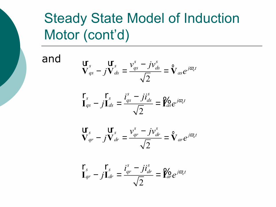
Steady State Model of Induction Motor (cont’d)
and°
2e
s ss s qs ds j tqs ds as
v jvj e ω−
− = =V V Vur ur
°2
e
s ss s qr dr j tqr dr ar
v jvj e ω−
− = =V V Vur ur
2e
s ss s qs ds j tqs ds as
i jij e ω−
− = =I I Ir r %
2e
s ss s qr dr j tqr dr ar
i jij e ω−
− = =I I Ir r %
Steady State Model of Induction Motor (cont’d)
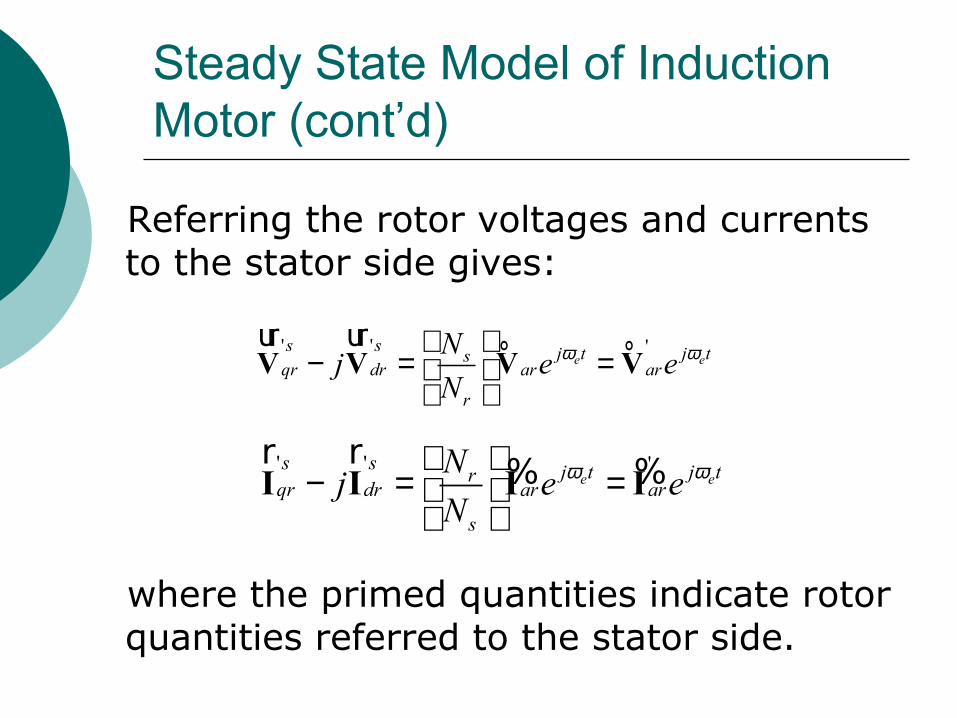
Referring the rotor voltages and currents to the stator side gives:
where the primed quantities indicate rotor quantities referred to the stator side.
° °' ' 'e e
s s j t j tsqr dr ar ar
r
Nj e e
Nω ω
− = =
V V V Vur ur
' ' 'e e
s s j t j trqr dr ar ar
s
Nj e e
Nω ω
− = =
I I I Ir r % %
Steady State Model of Induction Motor (cont’d)
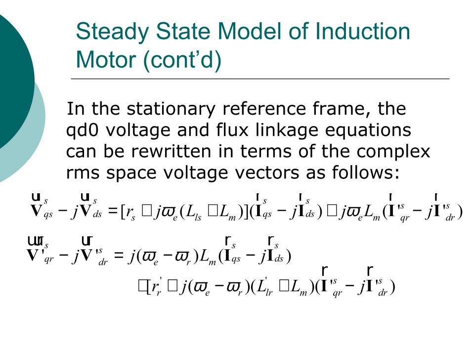
In the stationary reference frame, the qd0 voltage and flux linkage equations can be rewritten in terms of the complex rms space voltage vectors as follows:
[ ( )]( ) ( ' ' )s s s s s s
qs dsqs ds s e ls m e m qr drj r j L L j j L jω ω− = + + − + −V V I I I Iur ur r r r r
' ' ( ) ( )s s ss
qs dsqr dr e r mj j L jω ω− = − −V V I Iuur ur r r
' '[ ( )( )( ' ' )s sr e r lr m qr drr j L L jω ω+ + − + −I I
r r
Steady State Model of Induction Motor (cont’d)
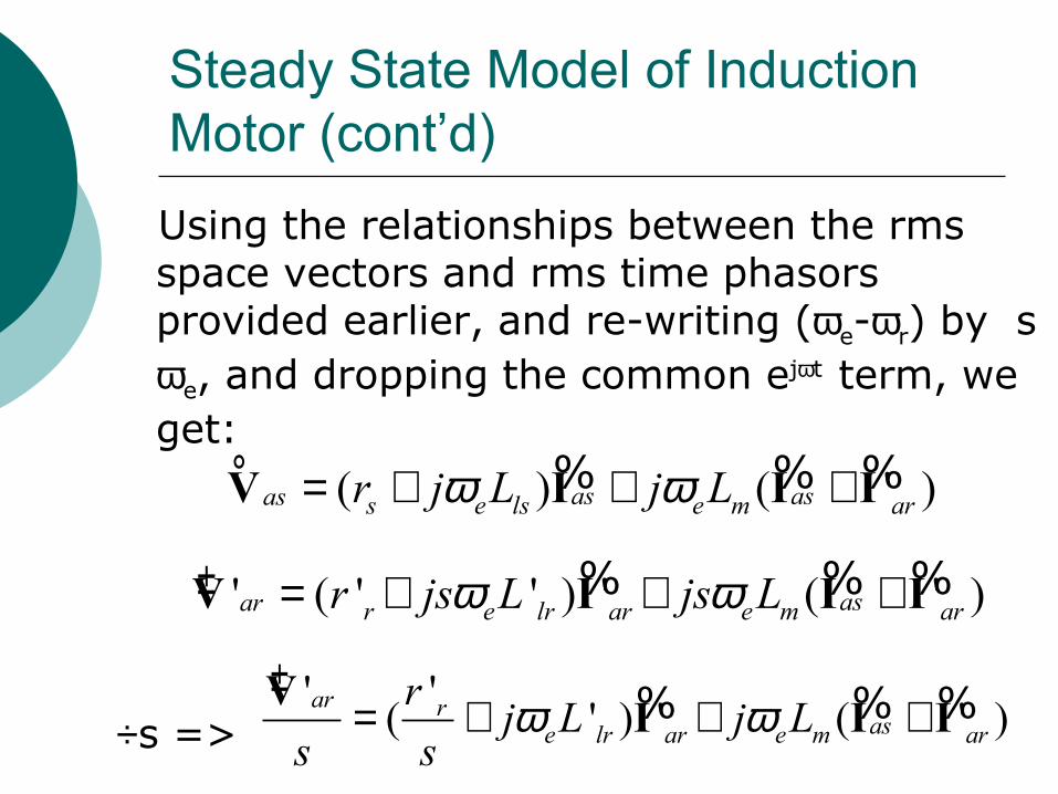
Using the relationships between the rms space vectors and rms time phasors provided earlier, and re-writing (ωe-ωr) by sωe, and dropping the common ejωt term, we get:
÷s =>
° ( ) ( ' )as asas s e ls e m arr j L j Lω ω= + + +V I I I% % %
± ' ( ' ' ) ' ( ' )asar r e lr ar e m arr js L js Lω ω= + + +V I I I% % %
± ''( ' ) ' ( ' )
ar rase lr ar e m ar
rj L j L
s sω ω= + + +V
I I I% % %
Steady State Model of Induction Motor (cont’d)
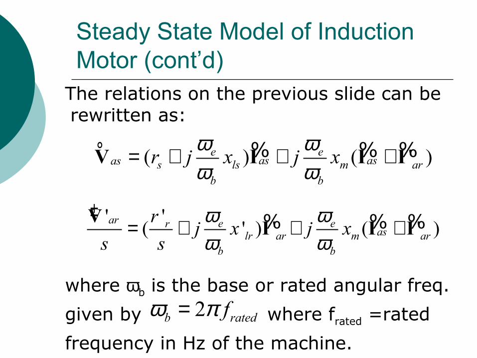
The relations on the previous slide can be rewritten as:
where ωb is the base or rated angular freq.
given by where frated =rated
frequency in Hz of the machine.
° ( ) ( ' )e eas asas s ls m ar
b b
r j x j xω ωω ω
= + + +V I I I% % %
± ''( ' ) ' ( ' )
ar e eraslr ar m ar
b b
rj x j x
s s
ω ωω ω
= + + +VI I I% % %
2b ratedfω π=
Steady State Model of Induction Motor (cont’d)
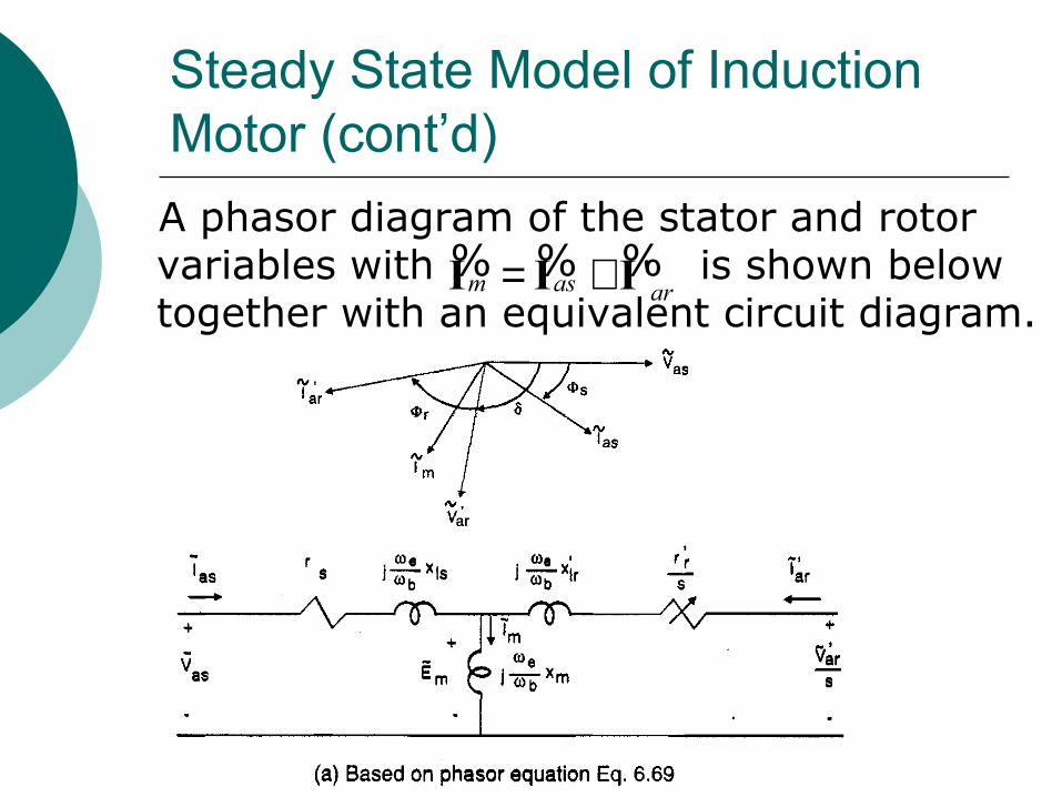
A phasor diagram of the stator and rotor variables with is shown below together with an equivalent circuit diagram.
'm as ar= +I I I% % %
Steady State Model of Induction Motor (cont’d)
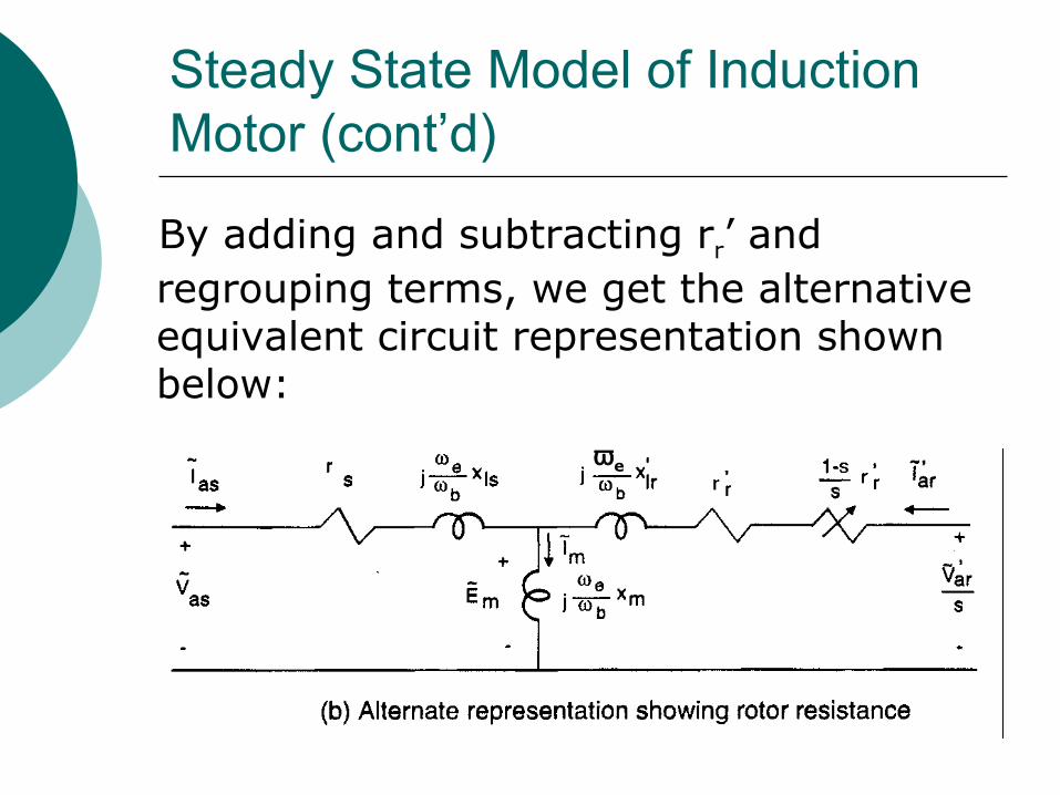
By adding and subtracting rr’ and regrouping terms, we get the alternative equivalent circuit representation shown below:
ωe
Steady State Model of Induction Motor (cont’d)
The rr’ (1-s)/s resistance term is associated with the mechanical power developed.
The rr’/s resistance term is associated with the power through the air gap.
Steady State Model of Induction Motor (cont’d)
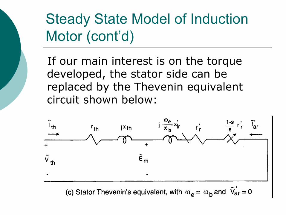
If our main interest is on the torque developed, the stator side can be replaced by the Thevenin equivalent circuit shown below:
Steady State Model of Induction Motor (cont’d)
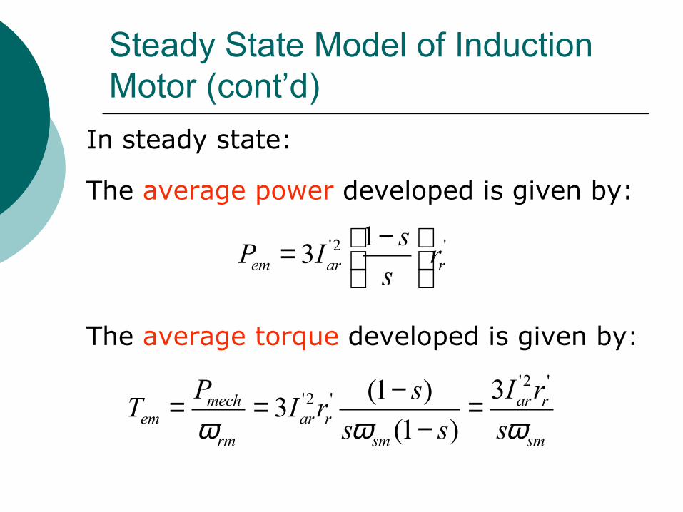
In steady state:
The average power developed is given by:
The average torque developed is given by:
'2 '13em ar r
sP I r
s
− =
'2 ''2 ' 3(1 )
3(1 )
mech ar rem ar r
rm sm sm
P I rsT I r
s s sω ω ω−= = =
−
Steady State Model of Induction Motor (cont’d)
The operating characteristics are quite different if the induction motor is operated at constant voltage or constant current.
Constant voltage -> stator series impedance drop is small => airgap voltage close to supply voltage over wide range of loading.
Constant current -> terminal and airgap voltage could vary significantly.
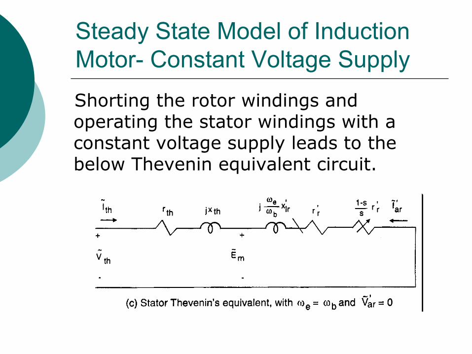
Steady State Model of Induction Motor- Constant Voltage Supply
Shorting the rotor windings and operating the stator windings with a constant voltage supply leads to the below Thevenin equivalent circuit.
Steady State Model of Induction Motor- Constant Voltage Supply
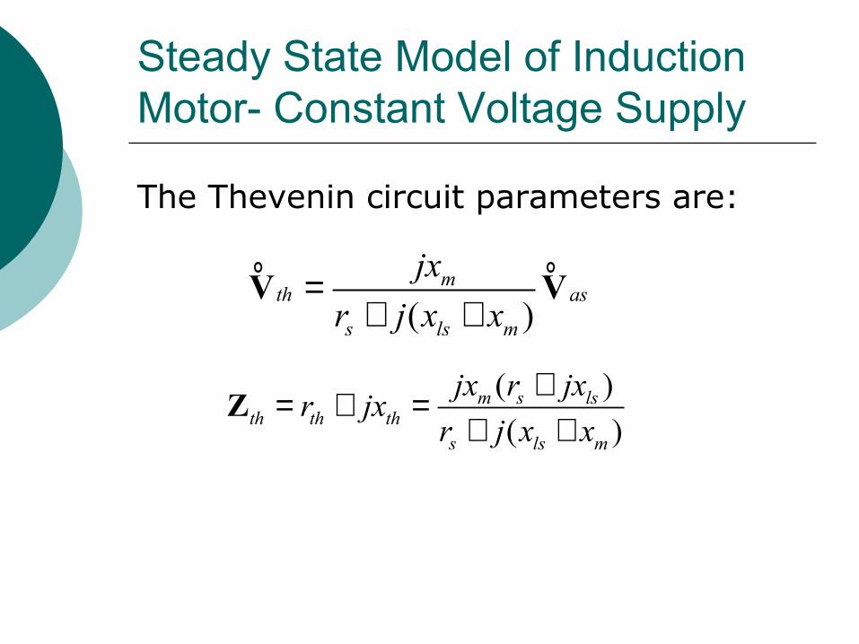
The Thevenin circuit parameters are:
° °( )
mth as
s ls m
jx
r j x x=
+ +V V
( )
( )m s ls
th th ths ls m
jx r jxr jx
r j x x
+= + =+ +
Z
Steady State Model of Induction Motor- Constant Voltage Supply
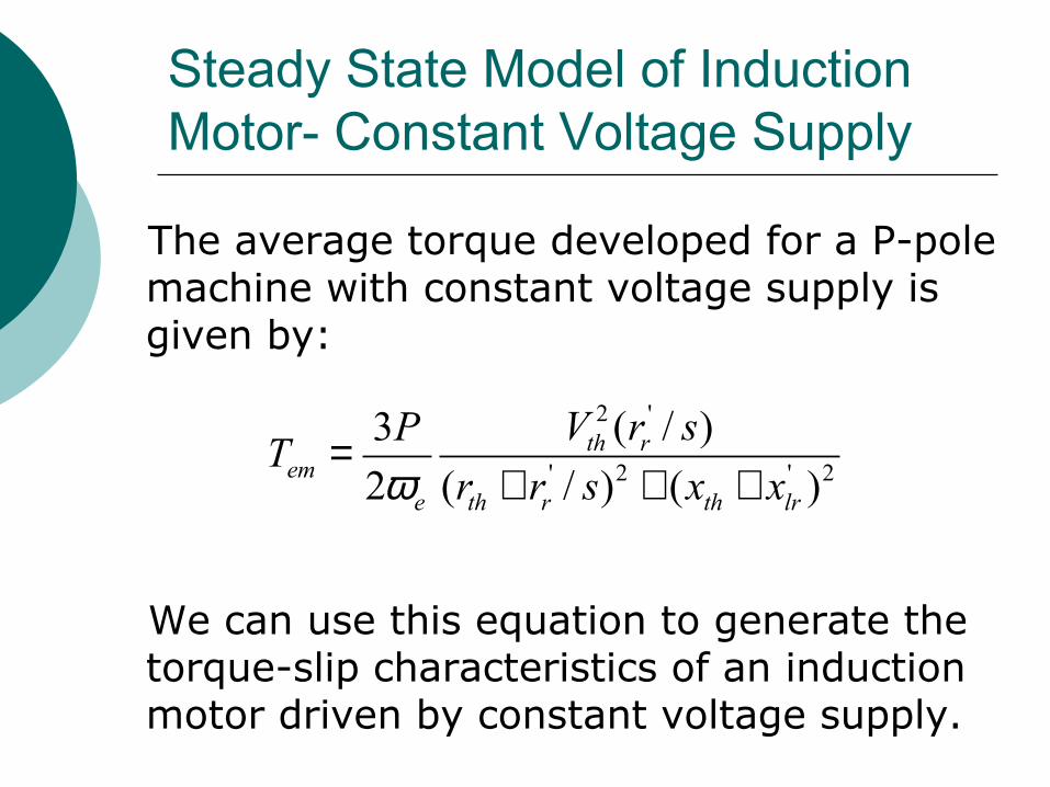
The average torque developed for a P-pole machine with constant voltage supply is given by:
We can use this equation to generate the torque-slip characteristics of an induction motor driven by constant voltage supply.
2 '
' 2 ' 2
( / )3
2 ( / ) ( )th r
eme th r th lr
V r sPT
r r s x xω=
+ + +
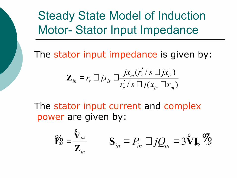
Steady State Model of Induction Motor- Stator Input Impedance
The stator input impedance is given by:
The stator input current and complex power are given by:
' '
' '
( / )
/ ( )m r lr
in s lsr lr m
jx r s jxr jx
r s j x x
+= + ++ +
Z
°as
as
in
= VIZ
% ° *3 asasin in inP jQ= + =S VΙ %
Steady State Model of Induction Motor- Constant Current Supply
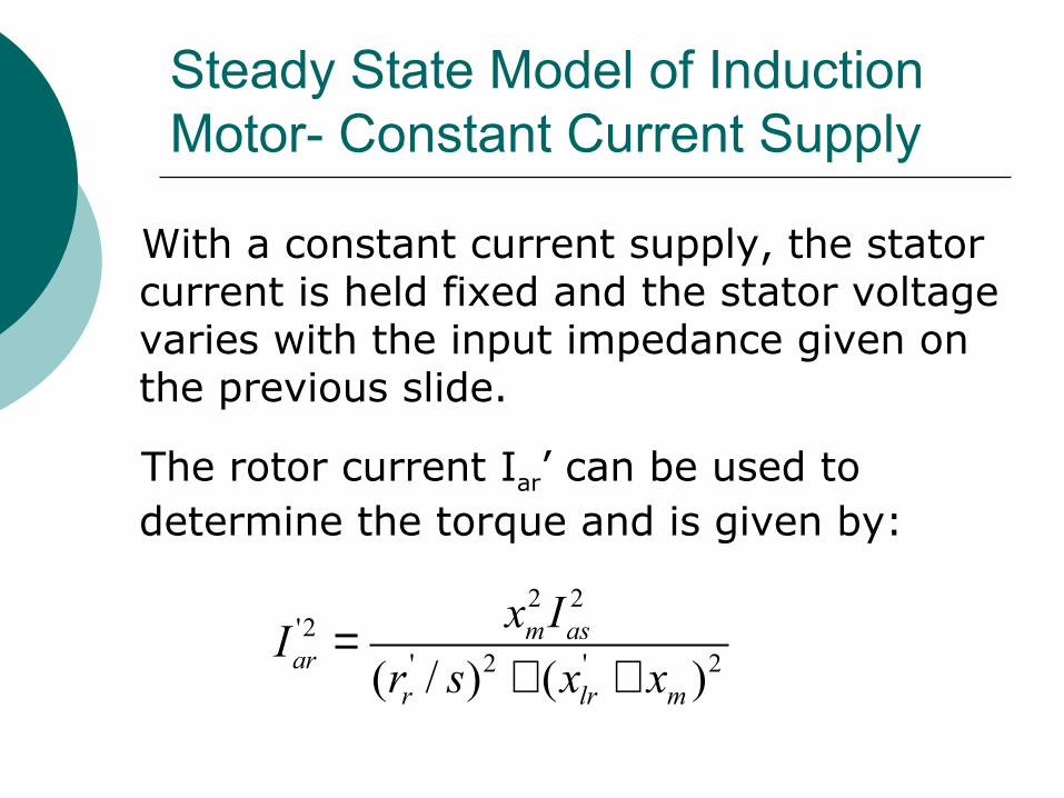
With a constant current supply, the stator current is held fixed and the stator voltage varies with the input impedance given on the previous slide.
The rotor current Iar’ can be used to determine the torque and is given by:
2 2'2
' 2 ' 2( / ) ( )m as
arr lr m
x II
r s x x=
+ +
Comparison of Constant Voltage vs. Constant Current Operation
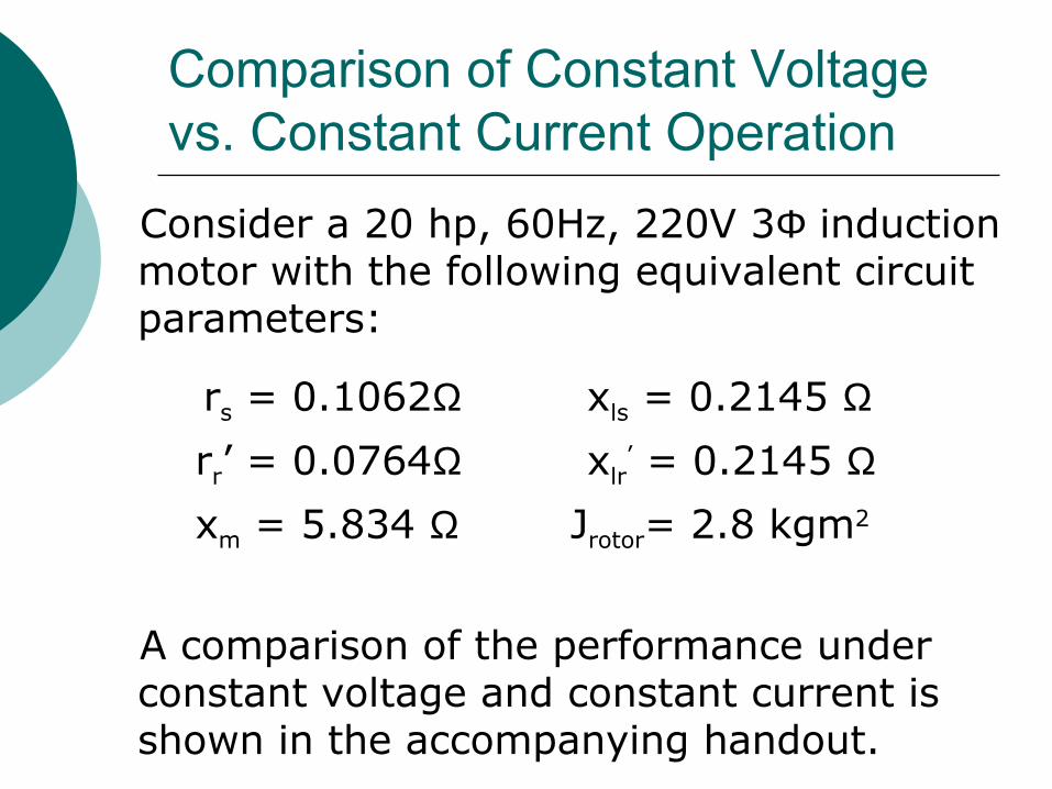
Consider a 20 hp, 60Hz, 220V 3Φ induction motor with the following equivalent circuit parameters:
rs = 0.1062Ω xls = 0.2145 Ω rr’ = 0.0764Ω xlr
’ = 0.2145 Ω xm = 5.834 Ω Jrotor= 2.8 kgm2
A comparison of the performance under constant voltage and constant current is shown in the accompanying handout.