Embed Size (px)
Citation preview
Nearshore Evaluation
October 15, 2013
Version 10.e
Page 88
13.1 History of Metric Monitoring
While Chl-a concentrations of the plankton in the open-water or pelagic zone of Lake
Tahoe has been sampled with some regularity (especially since 1984; TERC 2011), chlorophyll
data from the nearshore or littoral plankton is much less common and only exists as part of
limited, isolated studies.
Early Chl-a data from the nearshore is available in McGaughey et al. (1963) for pelagic
and nearshore sites around the lake. Between 1969 and 1975 the California-Nevada-Federal Joint
Water Quality Investigations program collected Chl-a at a combined total of 15 nearshore
stations (directly along the shoreline) and two deep-water limnetic sites (DWR 1971, 1972, 1973,
1974, 1975). Nearshore AGP was also measured in this program. Holm-Hansen (1976) made
measurements of Chl-a in the water column at a central pelagic station in Lake Tahoe in the mid-
1970s as part of a research study of lake characteristics. Leigh-Abbott et al. (1978) studied
chlorophyll a and temperature patterns along transects in the nearshore and offshore regions of
the lake in 1977. Paerl et al. (1976) looked at adenosine triphosphate (ATP) and Chl-a levels in
phytoplankton in Lake Tahoe from different depths, while Richerson et al. (1978) and Coon et
al. (1980) investigated the processes involved with formation of the deep chlorophyll maximum
in Lake Tahoe.
Recent monitoring using in situ fluorescence to estimate Chl-a also has been done by the
Desert Research Institute (DRI), both along the south shore and complete lake perimeters. The
later were achieved through numerous cruises that circumnavigated the lake within the littoral
zone, and which employed continuous measurements. Remote sensing data was used by
Steissberg et al. (2010) in a detailed analysis of spatial and seasonal patterns of distribution of
chlorophyll a in the upper euphotic zone of the nearshore. Recently (August 2011), researchers
with the U.S. EPA, TERC and DRI, circumnavigated the lake as part of the PARASOL study
(PARticulates And SOLutes in lakes) and took measurements of Chl-a (Kelly pers. comm.).
In summary, much more effort has been put into measuring Chl-a in the open-water,
pelagic portion of the Lake. Indeed, until the recent DRI continuous lake nearshore surveys,
direct measurement of chlorophyll a in the nearshore or littoral has been very limited with the
most comprehensive, historical monitoring coming from the early 1970s (DWR 1971-1975).
13.2 Monitoring Data Summary
13.2.1 Littoral Historic
An example of historical information from the California-Nevada-Federal Joint Water
Quality Investigations is chlorophyll a data at 12 nearshore sites reported for August 1971, May
1972, and August 1972 (DWR 1973), shown in Figure 13-1. Two pelagic stations (mid-lake
north and mid-lake south) also were simultaneously sampled. The full study occurred from
1969–1974.
Nearshore Evaluation
October 15, 2013
Version 10.e
Page 89
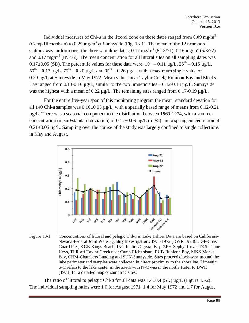
Individual measures of Chl-a in the littoral zone on these dates ranged from 0.09 mg/m3
(Camp Richardson) to 0.29 mg/m3 at Sunnyside (Fig. 13-1). The mean of the 12 nearshore
stations was uniform over the three sampling dates; 0.17 mg/m3 (8/18/71), 0.16 mg/m
3 (5/3/72)
and 0.17 mg/m3 (8/3/72). The mean concentration for all littoral sites on all sampling dates was
0.17±0.05 (SD). The percentile values for these data were: 10th
– 0.11 µg/L, 25th
– 0.15 µg/L,
50th
– 0.17 µg/L, 75th
– 0.20 µg/L and 95th
– 0.26 µg/L, with a maximum single value of
0.29 µg/L at Sunnyside in May 1972. Mean values near Taylor Creek, Rubicon Bay and Meeks
Bay ranged from 0.13-0.16 µg/L, similar to the two limnetic sites – 0.12-0.13 µg/L. Sunnyside
was the highest with a mean of 0.22 µg/L. The remaining sites ranged from 0.17-0.19 µg/L.
For the entire five-year span of this monitoring program the mean±standard devation for
all 140 Chl-a samples was 0.16±0.05 µg/L, with a spatially based range of means from 0.12-0.21
µg/L. There was a seasonal component to the distribution between 1969-1974, with a summer
concentration (mean±standard deviation) of 0.12±0.06 µg/L (n=52) and a spring concentration of
0.21±0.06 µg/L. Sampling over the course of the study was largely confined to single collections
in May and August.
Figure 13-1. Concentrations of littoral and pelagic Chl-a in Lake Tahoe. Data are based on California-
Nevada-Federal Joint Water Quality Investigations 1971-1972 (DWR 1973). CGP-Coast
Guard Pier, KGB-Kings Beach, INC-Incline/Crystal Bay, ZPH-Zephyr Cove, TKS-Tahoe
Keys, TLR-off Taylor Creek near Camp Richardson, RUB-Rubicon Bay, MKS-Meeks
Bay, CHM-Chambers Landing and SUN-Sunnyside. Sites proceed clock-wise around the
lake perimeter and samples were collected in direct proximity to the shoreline. Limnetic
S-C refers to the lake center in the south with N-C was in the north. Refer to DWR
(1973) for a detailed map of sampling sites.
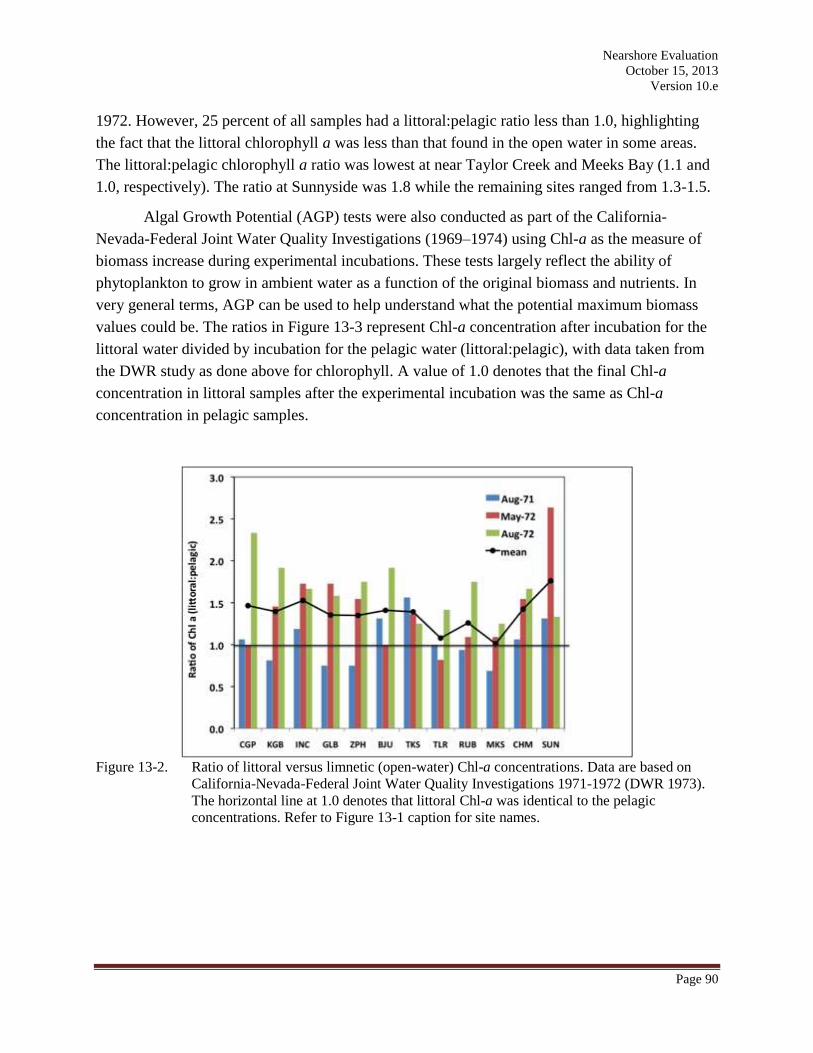
The ratio of littoral to pelagic Chl-a for all data was 1.4±0.4 (SD) µg/L (Figure 13-2).
The individual sampling ratios were 1.0 for August 1971, 1.4 for May 1972 and 1.7 for August
Nearshore Evaluation
October 15, 2013
Version 10.e
Page 90
1972. However, 25 percent of all samples had a littoral:pelagic ratio less than 1.0, highlighting
the fact that the littoral chlorophyll a was less than that found in the open water in some areas.
The littoral:pelagic chlorophyll a ratio was lowest at near Taylor Creek and Meeks Bay (1.1 and
1.0, respectively). The ratio at Sunnyside was 1.8 while the remaining sites ranged from 1.3-1.5.
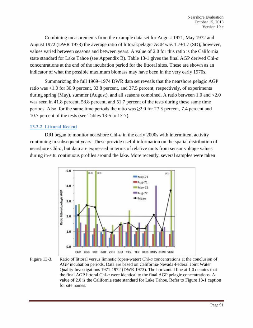
Algal Growth Potential (AGP) tests were also conducted as part of the California-
Nevada-Federal Joint Water Quality Investigations (1969–1974) using Chl-a as the measure of
biomass increase during experimental incubations. These tests largely reflect the ability of
phytoplankton to grow in ambient water as a function of the original biomass and nutrients. In
very general terms, AGP can be used to help understand what the potential maximum biomass
values could be. The ratios in Figure 13-3 represent Chl-a concentration after incubation for the
littoral water divided by incubation for the pelagic water (littoral:pelagic), with data taken from
the DWR study as done above for chlorophyll. A value of 1.0 denotes that the final Chl-a
concentration in littoral samples after the experimental incubation was the same as Chl-a
concentration in pelagic samples.
Figure 13-2. Ratio of littoral versus limnetic (open-water) Chl-a concentrations. Data are based on
California-Nevada-Federal Joint Water Quality Investigations 1971-1972 (DWR 1973).
The horizontal line at 1.0 denotes that littoral Chl-a was identical to the pelagic
concentrations. Refer to Figure 13-1 caption for site names.
Nearshore Evaluation
October 15, 2013
Version 10.e
Page 91
Combining measurements from the example data set for August 1971, May 1972 and
August 1972 (DWR 1973) the average ratio of littoral:pelagic AGP was 1.7±1.7 (SD); however,
values varied between seasons and between years. A value of 2.0 for this ratio is the California
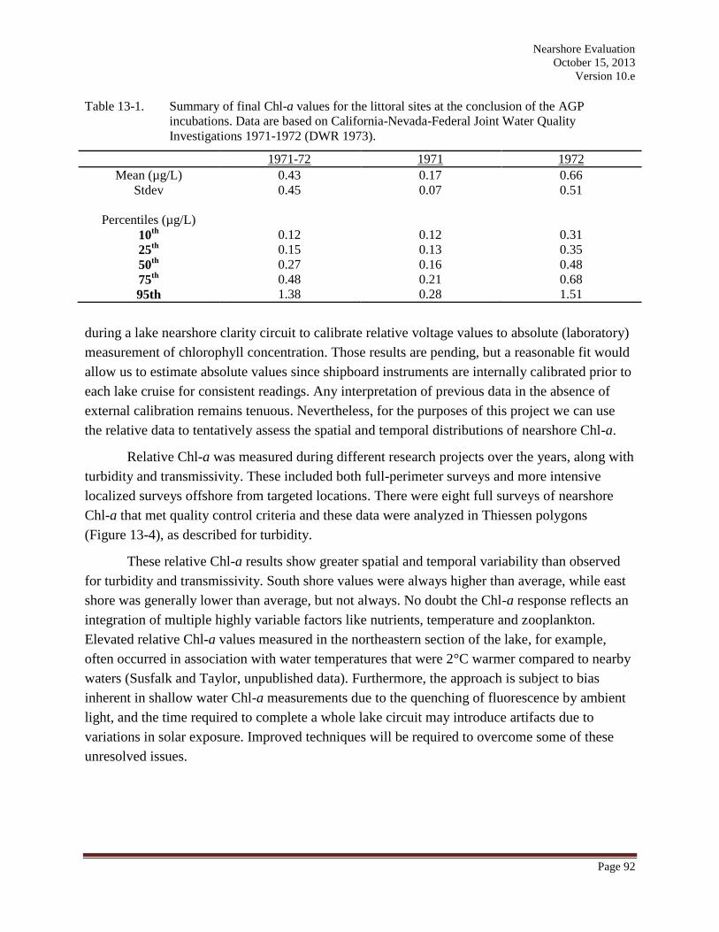
state standard for Lake Tahoe (see Appendix B). Table 13-1 gives the final AGP derived Chl-a
concentrations at the end of the incubation period for the littoral sites. These are shown as an
indicator of what the possible maximum biomass may have been in the very early 1970s.
Summarizing the full 1969–1974 DWR data set reveals that the nearshore:pelagic AGP
ratio was <1.0 for 30.9 percent, 33.8 percent, and 37.5 percent, respectively, of experiments
during spring (May), summer (August), and all seasons combined. A ratio between 1.0 and <2.0
was seen in 41.8 percent, 58.8 percent, and 51.7 percent of the tests during these same time
periods. Also, for the same time periods the ratio was ≥2.0 for 27.3 percent, 7.4 percent and
10.7 percent of the tests (see Tables 13-5 to 13-7).
13.2.2 Littoral Recent
DRI began to monitor nearshore Chl-a in the early 2000s with intermittent activity
continuing in subsequent years. These provide useful information on the spatial distribution of
nearshore Chl-a, but data are expressed in terms of relative units from sensor voltage values
during in-situ continuous profiles around the lake. More recently, several samples were taken
Figure 13-3. Ratio of littoral versus limnetic (open-water) Chl-a concentrations at the conclusion of
AGP incubation periods. Data are based on California-Nevada-Federal Joint Water
Quality Investigations 1971-1972 (DWR 1973). The horizontal line at 1.0 denotes that
the final AGP littoral Chl-a were identical to the final AGP pelagic concentrations. A
value of 2.0 is the California state standard for Lake Tahoe. Refer to Figure 13-1 caption
for site names.
Nearshore Evaluation
October 15, 2013
Version 10.e
Page 92
Table 13-1. Summary of final Chl-a values for the littoral sites at the conclusion of the AGP
incubations. Data are based on California-Nevada-Federal Joint Water Quality
Investigations 1971-1972 (DWR 1973).
1971-72 1971 1972
Mean (µg/L) 0.43 0.17 0.66
Stdev 0.45 0.07 0.51
Percentiles (µg/L)
10th
0.12 0.12 0.31
25th
0.15 0.13 0.35
50th
0.27 0.16 0.48
75th
0.48 0.21 0.68
95th 1.38 0.28 1.51
during a lake nearshore clarity circuit to calibrate relative voltage values to absolute (laboratory)
measurement of chlorophyll concentration. Those results are pending, but a reasonable fit would
allow us to estimate absolute values since shipboard instruments are internally calibrated prior to
each lake cruise for consistent readings. Any interpretation of previous data in the absence of
external calibration remains tenuous. Nevertheless, for the purposes of this project we can use
the relative data to tentatively assess the spatial and temporal distributions of nearshore Chl-a.
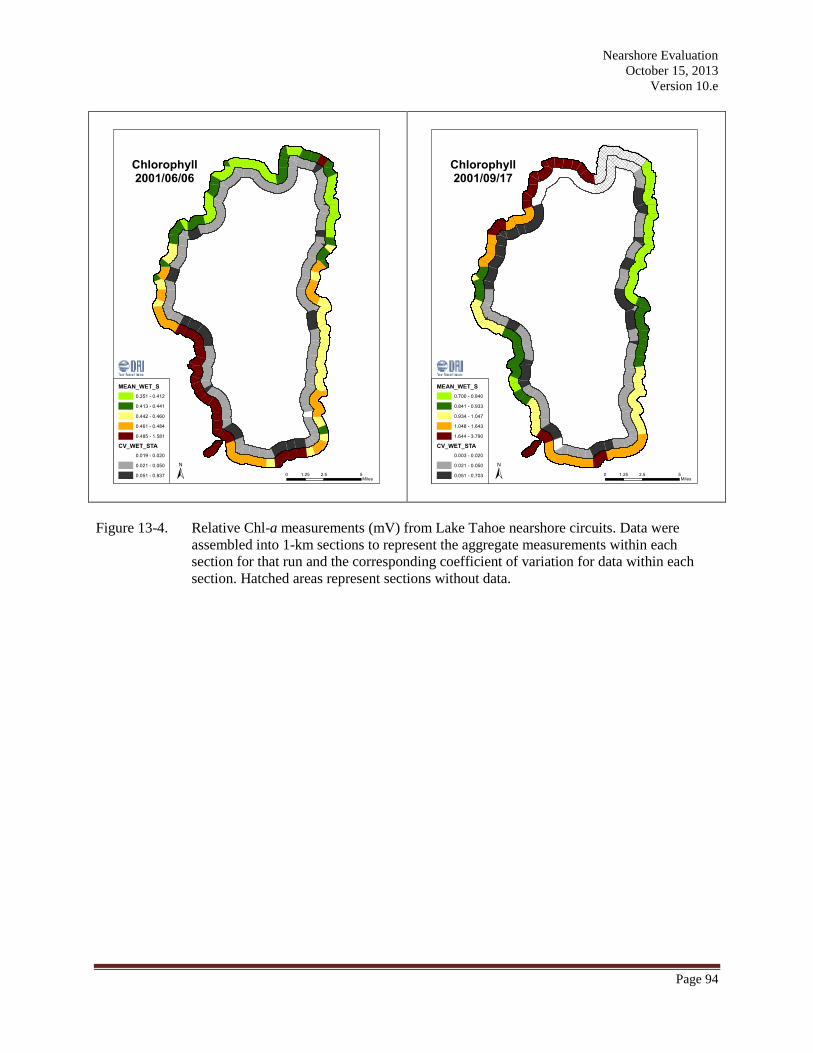
Relative Chl-a was measured during different research projects over the years, along with
turbidity and transmissivity. These included both full-perimeter surveys and more intensive
localized surveys offshore from targeted locations. There were eight full surveys of nearshore
Chl-a that met quality control criteria and these data were analyzed in Thiessen polygons
(Figure 13-4), as described for turbidity.
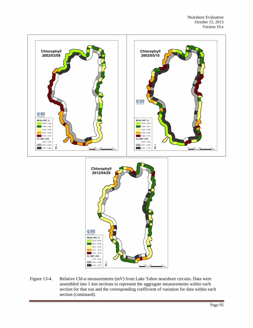
These relative Chl-a results show greater spatial and temporal variability than observed
for turbidity and transmissivity. South shore values were always higher than average, while east
shore was generally lower than average, but not always. No doubt the Chl-a response reflects an
integration of multiple highly variable factors like nutrients, temperature and zooplankton.
Elevated relative Chl-a values measured in the northeastern section of the lake, for example,
often occurred in association with water temperatures that were 2°C warmer compared to nearby
waters (Susfalk and Taylor, unpublished data). Furthermore, the approach is subject to bias
inherent in shallow water Chl-a measurements due to the quenching of fluorescence by ambient
light, and the time required to complete a whole lake circuit may introduce artifacts due to
variations in solar exposure. Improved techniques will be required to overcome some of these
unresolved issues.
Nearshore Evaluation
October 15, 2013
Version 10.e
Page 93
13.2.3 Whole Lake Satellite
In general, but depending on location, MODIS-derived Chl-a 1 during 2002-2010 was
higher in the nearshore relative to pelagic regions (Figure 13-5 provides an example from
Steissberg et al. 2010). Leigh-Abbott et al. (1978) found greater variability in Chl-a levels in the
nearshore and reported that large-scale patterns were dominated by stream inflow of nutrients
and by possible upwelling events created by the particular exposure and wind patterns of the
area. Physical processes such as gyres, eddies and upwelling affect the movement of Chl-a in the
lake and impact seasonal patterns of distribution. Elevated concentrations of Chl-a appear to
spread around the lake via large-scale circulation (gyres), with flow reversals and shore-to-shore
(south-to-south or south-to-west) transport via smaller-scale (“spiral”) eddies 3-5 km in diameter
(Steissberg et al., 2010). Chl-a was observed to spread offshore in plumes or jets following
upwelling events. The plumes and eddies may contribute to offshore diffusion. Strong upwelling
can transport high clarity water to the surface, which contains low levels of particles but high
levels of nutrients.
1 MODIS (Moderate Resolution Imaging Spectroradiometer) is a remote sensing technology supported by NASA.
Using algorithms specifically created for Lake Tahoe, Steissberg et al. (2010) was able to re-create chlorophyll a
levels synoptically throughout the lake including both nearshore and open-water.
Nearshore Evaluation
October 15, 2013
Version 10.e
Page 94
Figure 13-4. Relative Chl-a measurements (mV) from Lake Tahoe nearshore circuits. Data were
assembled into 1-km sections to represent the aggregate measurements within each
section for that run and the corresponding coefficient of variation for data within each
section. Hatched areas represent sections without data.
Nearshore Evaluation
October 15, 2013
Version 10.e
Page 95
Figure 13-4. Relative Chl-a measurements (mV) from Lake Tahoe nearshore circuits. Data were
assembled into 1-km sections to represent the aggregate measurements within each
section for that run and the corresponding coefficient of variation for data within each
section (continued).
Nearshore Evaluation
October 15, 2013
Version 10.e
Page 96
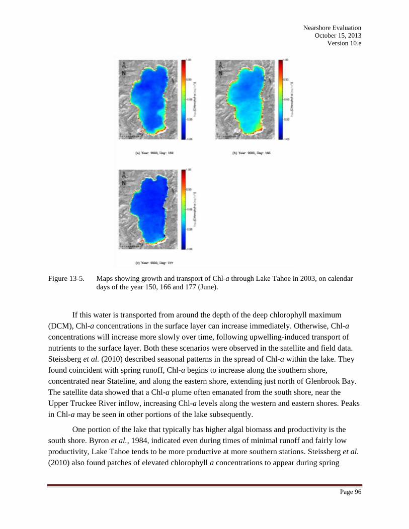
Figure 13-5. Maps showing growth and transport of Chl-a through Lake Tahoe in 2003, on calendar
days of the year 150, 166 and 177 (June).
If this water is transported from around the depth of the deep chlorophyll maximum
(DCM), Chl-a concentrations in the surface layer can increase immediately. Otherwise, Chl-a
concentrations will increase more slowly over time, following upwelling-induced transport of
nutrients to the surface layer. Both these scenarios were observed in the satellite and field data.
Steissberg et al. (2010) described seasonal patterns in the spread of Chl-a within the lake. They
found coincident with spring runoff, Chl-a begins to increase along the southern shore,
concentrated near Stateline, and along the eastern shore, extending just north of Glenbrook Bay.
The satellite data showed that a Chl-a plume often emanated from the south shore, near the
Upper Truckee River inflow, increasing Chl-a levels along the western and eastern shores. Peaks
in Chl-a may be seen in other portions of the lake subsequently.
One portion of the lake that typically has higher algal biomass and productivity is the
south shore. Byron et al., 1984, indicated even during times of minimal runoff and fairly low
productivity, Lake Tahoe tends to be more productive at more southern stations. Steissberg et al.
(2010) also found patches of elevated chlorophyll a concentrations to appear during spring
Nearshore Evaluation
October 15, 2013
Version 10.e
Page 97
runoff which appeared to be concentrated along the southern shore adjacent to the Upper
Truckee River, Trout Creek and Edgewood Creek inflows.
Monitoring during PARASOL studies in August of 2011 also showed increased Chl-a
along a portion of south shore near the Upper Truckee plume (Figures 13-6 and 13-7). The lower
water quality observed along the southeast portion of south shore may be due to currents
transporting the Upper Truckee River and Trout Creek inputs eastward. In addition, there may be
significant sediment resuspension from the shoals, which are only approximately 2 m deep
between the Trout Creek and Edgewood Creek inflows, which may be transported eastward.
Surface current analysis from satellite images and drogue data indicate that a spiral eddy is often
found in the southeast corner of the lake. This eddy may concentrate and retain nutrients in this
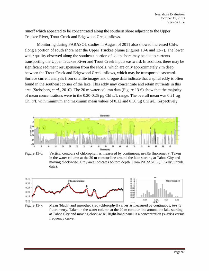
area (Steissberg et al., 2010). The 20 m water column data (Figure 13-6) show that the majority
of mean concentrations were in the 0.20-0.25 µg Chl a/L range. The overall mean was 0.21 µg
Chl a/L with minimum and maximum mean values of 0.12 and 0.30 µg Chl a/L, respectively.
Figure 13-6. Vertical contours of chlorophyll as measured by continuous, in-situ fluorometry. Taken
in the water column at the 20 m contour line around the lake starting at Tahoe City and
moving clock-wise. Grey area indicates bottom depth. From PARASOL (J. Kelly, unpub.
data).
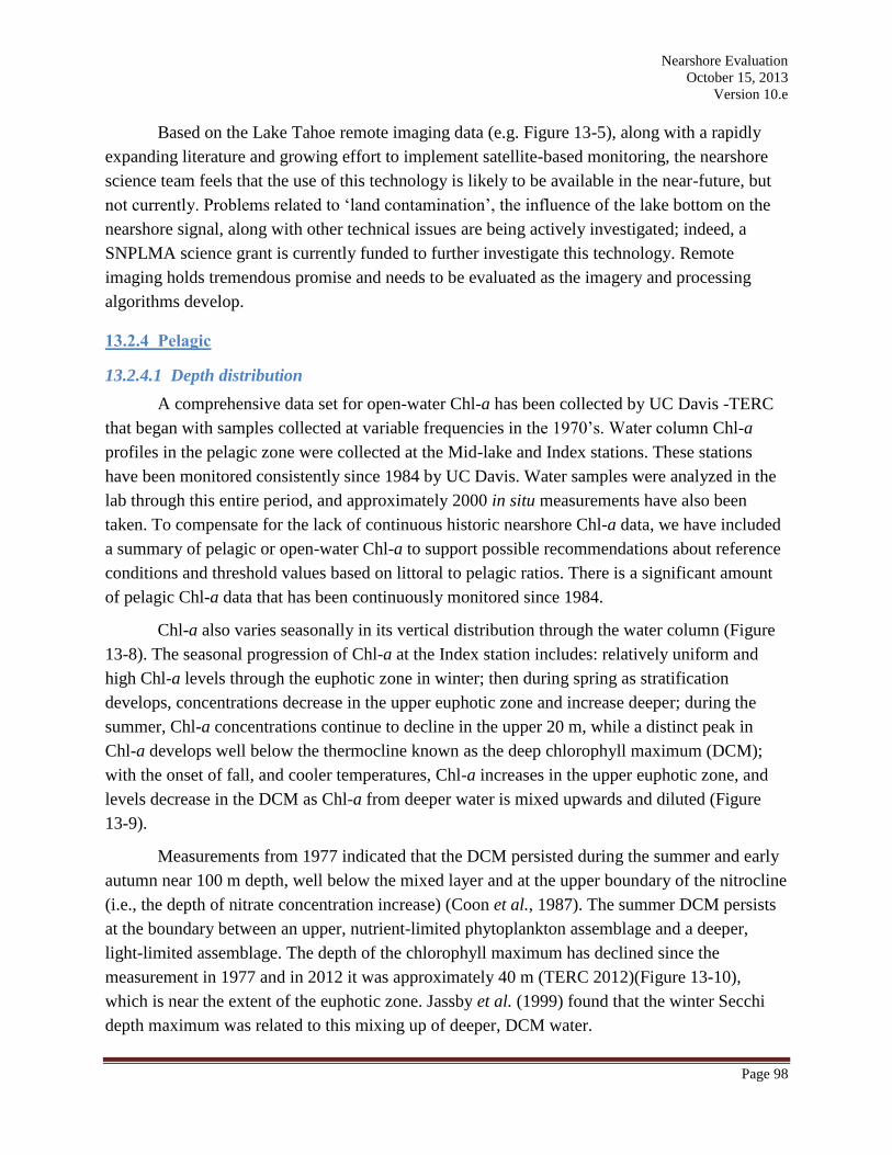
Figure 13-7. Mean (black) and smoothed (red) chlorophyll values as measured by continuous, in-site
fluorometry. Taken in the water column at the 20 m contour line around the lake starting
at Tahoe City and moving clock-wise. Right-hand panel is a concentration (x-axis) versus
frequency curve.
Nearshore Evaluation
October 15, 2013
Version 10.e
Page 98
Based on the Lake Tahoe remote imaging data (e.g. Figure 13-5), along with a rapidly
expanding literature and growing effort to implement satellite-based monitoring, the nearshore
science team feels that the use of this technology is likely to be available in the near-future, but
not currently. Problems related to ‘land contamination’, the influence of the lake bottom on the
nearshore signal, along with other technical issues are being actively investigated; indeed, a
SNPLMA science grant is currently funded to further investigate this technology. Remote
imaging holds tremendous promise and needs to be evaluated as the imagery and processing
algorithms develop.
13.2.4 Pelagic
13.2.4.1 Depth distribution
A comprehensive data set for open-water Chl-a has been collected by UC Davis -TERC
that began with samples collected at variable frequencies in the 1970’s. Water column Chl-a
profiles in the pelagic zone were collected at the Mid-lake and Index stations. These stations
have been monitored consistently since 1984 by UC Davis. Water samples were analyzed in the
lab through this entire period, and approximately 2000 in situ measurements have also been
taken. To compensate for the lack of continuous historic nearshore Chl-a data, we have included
a summary of pelagic or open-water Chl-a to support possible recommendations about reference
conditions and threshold values based on littoral to pelagic ratios. There is a significant amount
of pelagic Chl-a data that has been continuously monitored since 1984.
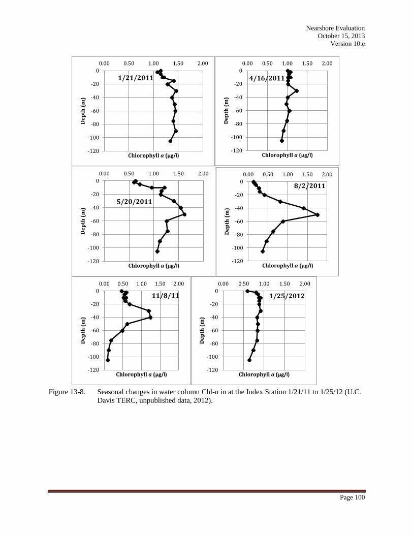
Chl-a also varies seasonally in its vertical distribution through the water column (Figure
13-8). The seasonal progression of Chl-a at the Index station includes: relatively uniform and
high Chl-a levels through the euphotic zone in winter; then during spring as stratification
develops, concentrations decrease in the upper euphotic zone and increase deeper; during the
summer, Chl-a concentrations continue to decline in the upper 20 m, while a distinct peak in
Chl-a develops well below the thermocline known as the deep chlorophyll maximum (DCM);
with the onset of fall, and cooler temperatures, Chl-a increases in the upper euphotic zone, and
levels decrease in the DCM as Chl-a from deeper water is mixed upwards and diluted (Figure
13-9).
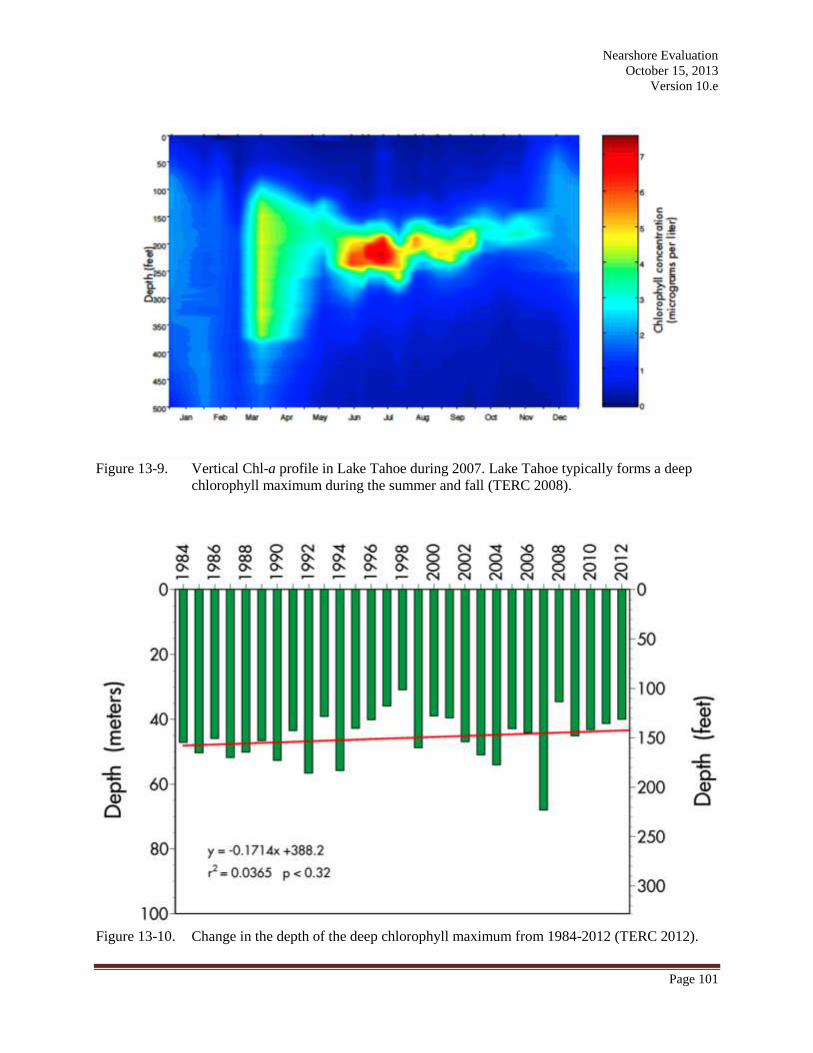
Measurements from 1977 indicated that the DCM persisted during the summer and early
autumn near 100 m depth, well below the mixed layer and at the upper boundary of the nitrocline
(i.e., the depth of nitrate concentration increase) (Coon et al., 1987). The summer DCM persists
at the boundary between an upper, nutrient-limited phytoplankton assemblage and a deeper,
light-limited assemblage. The depth of the chlorophyll maximum has declined since the
measurement in 1977 and in 2012 it was approximately 40 m (TERC 2012)(Figure 13-10),
which is near the extent of the euphotic zone. Jassby et al. (1999) found that the winter Secchi
depth maximum was related to this mixing up of deeper, DCM water.
Nearshore Evaluation
October 15, 2013
Version 10.e
Page 99
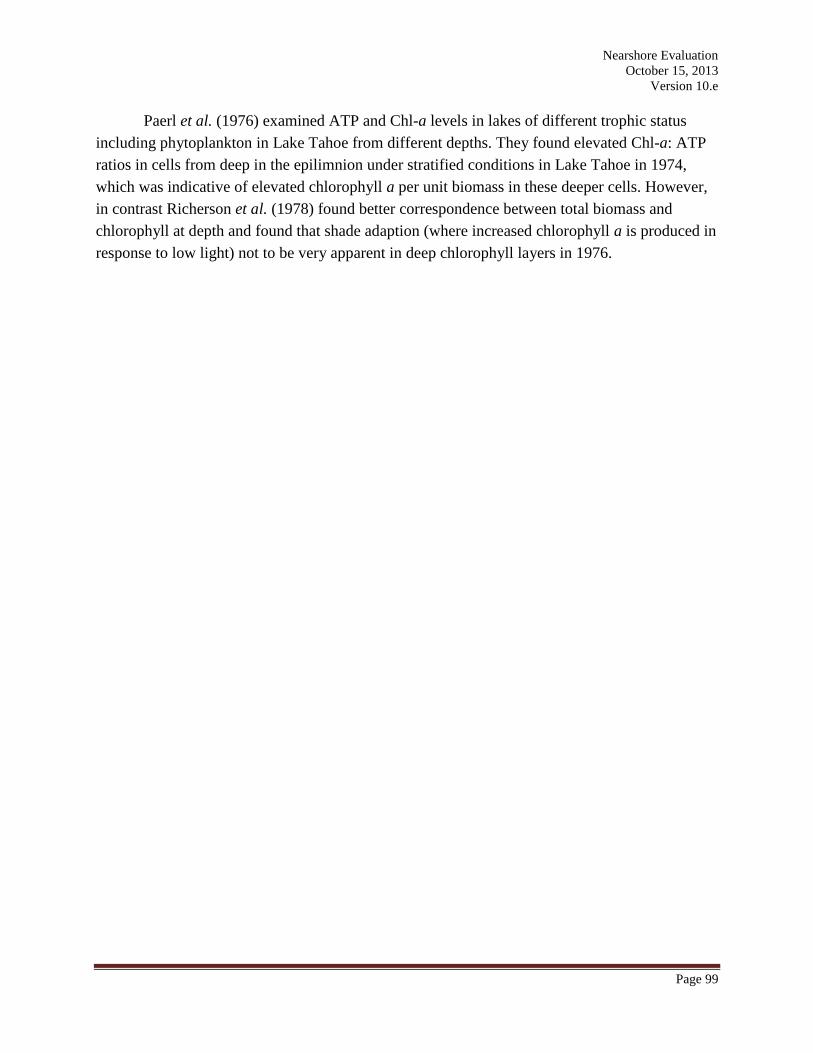
Paerl et al. (1976) examined ATP and Chl-a levels in lakes of different trophic status
including phytoplankton in Lake Tahoe from different depths. They found elevated Chl-a: ATP
ratios in cells from deep in the epilimnion under stratified conditions in Lake Tahoe in 1974,
which was indicative of elevated chlorophyll a per unit biomass in these deeper cells. However,
in contrast Richerson et al. (1978) found better correspondence between total biomass and
chlorophyll at depth and found that shade adaption (where increased chlorophyll a is produced in
response to low light) not to be very apparent in deep chlorophyll layers in 1976.
Nearshore Evaluation
October 15, 2013
Version 10.e
Page 100
Figure 13-8. Seasonal changes in water column Chl-a in at the Index Station 1/21/11 to 1/25/12 (U.C.
Davis TERC, unpublished data, 2012).
-120
-100
-80
-60
-40
-20
0
0.00 0.50 1.00 1.50 2.00
De
pth
(m
)
Chlorophyll a (µg/l)
1/21/2011
-120
-100
-80
-60
-40
-20
0
0.00 0.50 1.00 1.50 2.00
De
pth
(m
)
Chlorophyll a (µg/l)
4/16/2011
-120
-100
-80
-60
-40
-20
0
0.00 0.50 1.00 1.50 2.00
De
pth
(m
)
Chlorophyll a (µg/l)
5/20/2011
-120
-100
-80
-60
-40
-20
0
0.00 0.50 1.00 1.50 2.00
De
pth
(m
)
Chlorophyll a (µg/l)
8/2/2011
-120
-100
-80
-60
-40
-20
0
0.00 0.50 1.00 1.50 2.00
De
pth
(m
)
Chlorophyll a (µg/l)
11/8/11
-120
-100
-80
-60
-40
-20
0
0.00 0.50 1.00 1.50 2.00
De
pth
(m
)
Chlorophyll a (µg/l)
1/25/2012
Nearshore Evaluation
October 15, 2013
Version 10.e
Page 101
Figure 13-9. Vertical Chl-a profile in Lake Tahoe during 2007. Lake Tahoe typically forms a deep
chlorophyll maximum during the summer and fall (TERC 2008).
Figure 13-10. Change in the depth of the deep chlorophyll maximum from 1984-2012 (TERC 2012).
Nearshore Evaluation
October 15, 2013
Version 10.e
Page 102
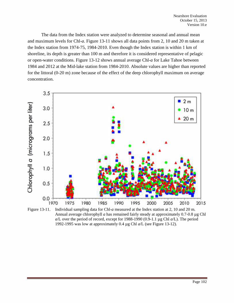
The data from the Index station were analyzed to determine seasonal and annual mean
and maximum levels for Chl-a. Figure 13-11 shows all data points from 2, 10 and 20 m taken at
the Index station from 1974-75, 1984-2010. Even though the Index station is within 1 km of
shoreline, its depth is greater than 100 m and therefore it is considered representative of pelagic
or open-water conditions. Figure 13-12 shows annual average Chl-a for Lake Tahoe between
1984 and 2012 at the Mid-lake station from 1984-2010. Absolute values are higher than reported
for the littoral (0-20 m) zone because of the effect of the deep chlorophyll maximum on average
concentration.
Figure 13-11. Individual sampling data for Chl-a measured at the Index station at 2, 10 and 20 m.
Annual average chlorophyll a has remained fairly steady at approximately 0.7-0.8 µg Chl
a/L over the period of record, except for 1988-1990 (0.9-1.1 µg Chl a/L). The period
1992-1995 was low at approximately 0.4 µg Chl a/L (see Figure 13-12).
Nearshore Evaluation
October 15, 2013
Version 10.e
Page 103
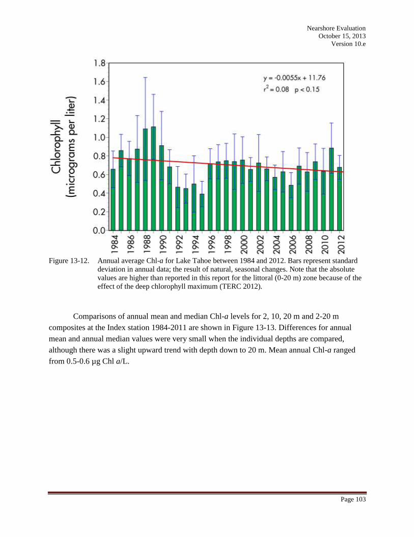
Figure 13-12. Annual average Chl-a for Lake Tahoe between 1984 and 2012. Bars represent standard
deviation in annual data; the result of natural, seasonal changes. Note that the absolute
values are higher than reported in this report for the littoral (0-20 m) zone because of the
effect of the deep chlorophyll maximum (TERC 2012).
Comparisons of annual mean and median Chl-a levels for 2, 10, 20 m and 2-20 m
composites at the Index station 1984-2011 are shown in Figure 13-13. Differences for annual
mean and annual median values were very small when the individual depths are compared,
although there was a slight upward trend with depth down to 20 m. Mean annual Chl-a ranged
from 0.5-0.6 µg Chl a/L.
Nearshore Evaluation
October 15, 2013
Version 10.e
Page 104
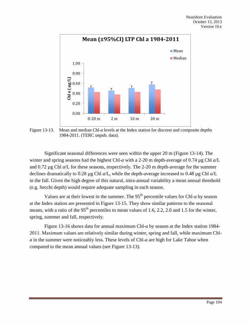
Figure 13-13. Mean and median Chl-a levels at the Index station for discreet and composite depths
1984-2011. (TERC unpub. data).
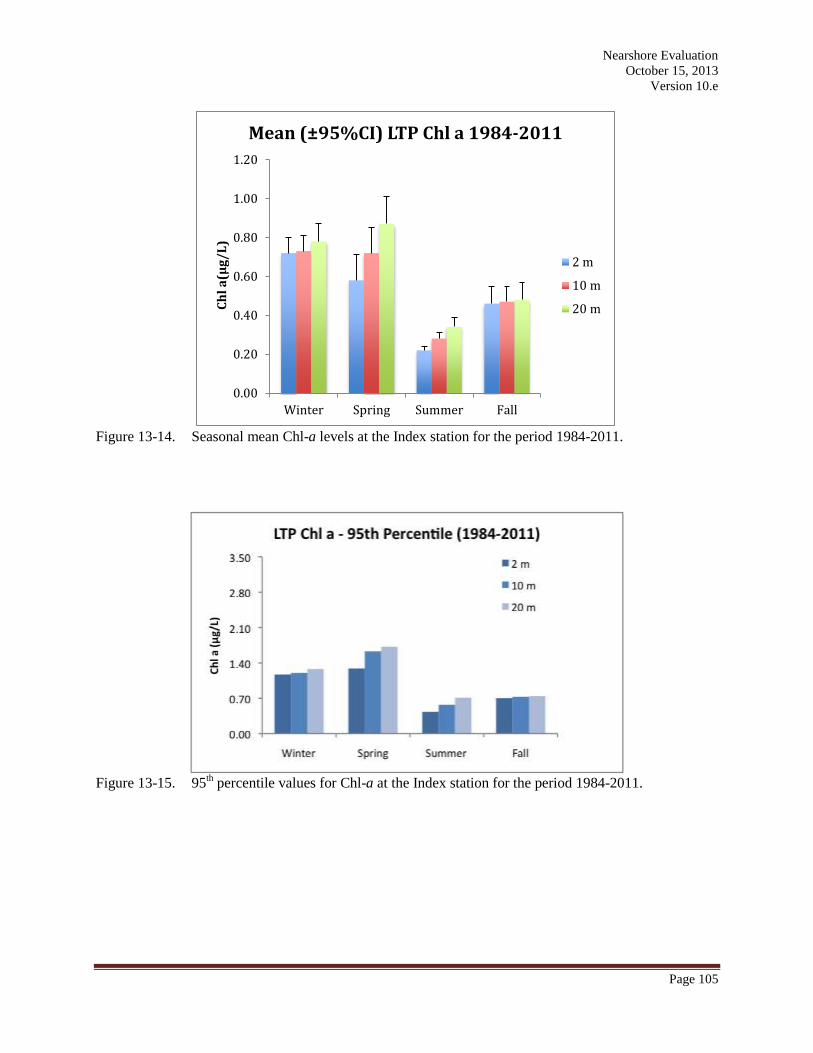
Significant seasonal differences were seen within the upper 20 m (Figure 13-14). The
winter and spring seasons had the highest Chl-a with a 2-20 m depth-average of 0.74 µg Chl a/L
and 0.72 µg Chl a/L for these seasons, respectively. The 2-20 m depth-average for the summer
declines dramatically to 0.28 µg Chl a/L, while the depth-average increased to 0.48 µg Chl a/L
in the fall. Given the high degree of this natural, intra-annual variability a mean annual threshold
(e.g. Secchi depth) would require adequate sampling in each season.
Values are at their lowest in the summer. The 95th
percentile values for Chl-a by season
at the Index station are presented in Figure 13-15. They show similar patterns to the seasonal
means, with a ratio of the 95th
percentiles to mean values of 1.6, 2.2, 2.0 and 1.5 for the winter,
spring, summer and fall, respectively.
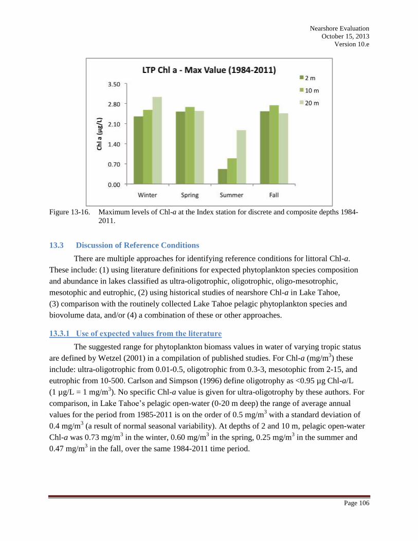
Figure 13-16 shows data for annual maximum Chl-a by season at the Index station 1984-
2011. Maximum values are relatively similar during winter, spring and fall, while maximum Chl-
a in the summer were noticeably less. These levels of Chl-a are high for Lake Tahoe when
compared to the mean annual values (see Figure 13-13).
0.00
0.20
0.40
0.60
0.80
1.00
0-20 m 2 m 10 m 20 m
Ch
l a
( µ
g/
L)
Mean (±95%CI) LTP Chl a 1984-2011
Mean
Median
Nearshore Evaluation
October 15, 2013
Version 10.e
Page 105
Figure 13-14. Seasonal mean Chl-a levels at the Index station for the period 1984-2011.
Figure 13-15. 95
th percentile values for Chl-a at the Index station for the period 1984-2011.
0.00
0.20
0.40
0.60
0.80
1.00
1.20
Winter Spring Summer Fall
Ch
l a
(µg
/L
)
Mean (±95%CI) LTP Chl a 1984-2011
2 m
10 m
20 m
Nearshore Evaluation
October 15, 2013
Version 10.e
Page 106
Figure 13-16. Maximum levels of Chl-a at the Index station for discrete and composite depths 1984-
2011.
13.3 Discussion of Reference Conditions
There are multiple approaches for identifying reference conditions for littoral Chl-a.
These include: (1) using literature definitions for expected phytoplankton species composition
and abundance in lakes classified as ultra-oligotrophic, oligotrophic, oligo-mesotrophic,
mesotophic and eutrophic, (2) using historical studies of nearshore Chl-a in Lake Tahoe,
(3) comparison with the routinely collected Lake Tahoe pelagic phytoplankton species and
biovolume data, and/or (4) a combination of these or other approaches.
13.3.1 Use of expected values from the literature
The suggested range for phytoplankton biomass values in water of varying tropic status
are defined by Wetzel (2001) in a compilation of published studies. For Chl-a (mg/m3) these
include: ultra-oligotrophic from 0.01-0.5, oligotrophic from 0.3-3, mesotophic from 2-15, and
eutrophic from 10-500. Carlson and Simpson (1996) define oligotrophy as <0.95 µg Chl-a/L
(1 µg/L = 1 mg/m3). No specific Chl-a value is given for ultra-oligotrophy by these authors. For
comparison, in Lake Tahoe’s pelagic open-water (0-20 m deep) the range of average annual
values for the period from 1985-2011 is on the order of 0.5 mg/m3 with a standard deviation of
0.4 mg/m3 (a result of normal seasonal variability). At depths of 2 and 10 m, pelagic open-water
Chl-a was 0.73 mg/m3 in the winter, 0.60 mg/m
3 in the spring, 0.25 mg/m
3 in the summer and
0.47 mg/m3 in the fall, over the same 1984-2011 time period.
Nearshore Evaluation
October 15, 2013
Version 10.e
Page 107
13.3.2 Use of historic littoral zone data from a time when lake conditions were more
desirable
The period from the late 1960s to early 1970s, for which littoral Chl-a data are available,
was characterized by better water quality condition than we see today. For example, annual
average Secchi depth was on the order of 28-30 m and significantly better than the ~20 m value
of recent years (TERC 2011). Indeed, the California state standard for transparency was based on
the 1968-1971 period. The pelagic Chl-a in the early 1970s was typically in the range of
0.10-0.20 µg/L, whereas today the values have increased to 0.50-0.60 µg/L.
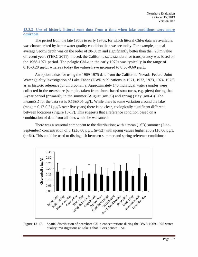
An option exists for using the 1969-1975 data from the California-Nevada-Federal Joint
Water Quality Investigation of Lake Tahoe (DWR publications in 1971, 1972, 1973, 1974, 1975)
as an historic reference for chlorophyll a. Approximately 140 individual water samples were
collected in the nearshore (samples taken from shore-based structures, e.g. piers) during that
5-year period (primarily in the summer (August (n=52)) and spring (May (n=64)). The
mean±SD for the data set is 0.16±0.05 µg/L. While there is some variation around the lake
(range = 0.12-0.21 µg/L over five years) there is no clear, ecologically significant different
between locations (Figure 13-17). This suggests that a reference condition based on a
combination of data from all sites would be warranted.
There was a seasonal component to the distribution; with a mean (±SD) summer (June-
September) concentration of 0.12±0.06 µg/L (n=52) with spring values higher at 0.21±0.06 µg/L
(n=64). This could be used to distinguish between summer and spring reference conditions.
Figure 13-17. Spatial distribution of nearshore Chl-a concentrations during the DWR 1969-1975 water
quality investigations at Lake Tahoe. Bars denote 1 SD.
Nearshore Evaluation
October 15, 2013
Version 10.e
Page 108
While means are very useful as measures of central tendency, they may or may not be
fully representative for use in establishing reference conditions. For example, samples collected
from the Tahoe Keys site during mid-summer (8/26/70 and 8/18/71) had chlorophyll levels of
0.05 and 0.25 µg/L, respectively. If the 5-year mean of 0.16 µg/L were used as the reference
condition, then 0.25 µg/L would exceed the reference condition.
The use of a single maximum value would also be non-representative as it may be much
higher than the majority of observed values, e.g. the observed value of 0.39 µg/L at Stateline
South on 5/8/74. However, if we take each of the maximum values from each sampling trip, as
well as the summer and spring dates independently, the mean of maximum values are: for All
Data = 0.23±0.10 µg/L, for Summer = 0.18±0.07 µg/L, and for Spring = 0.28±0.11 µg/L.
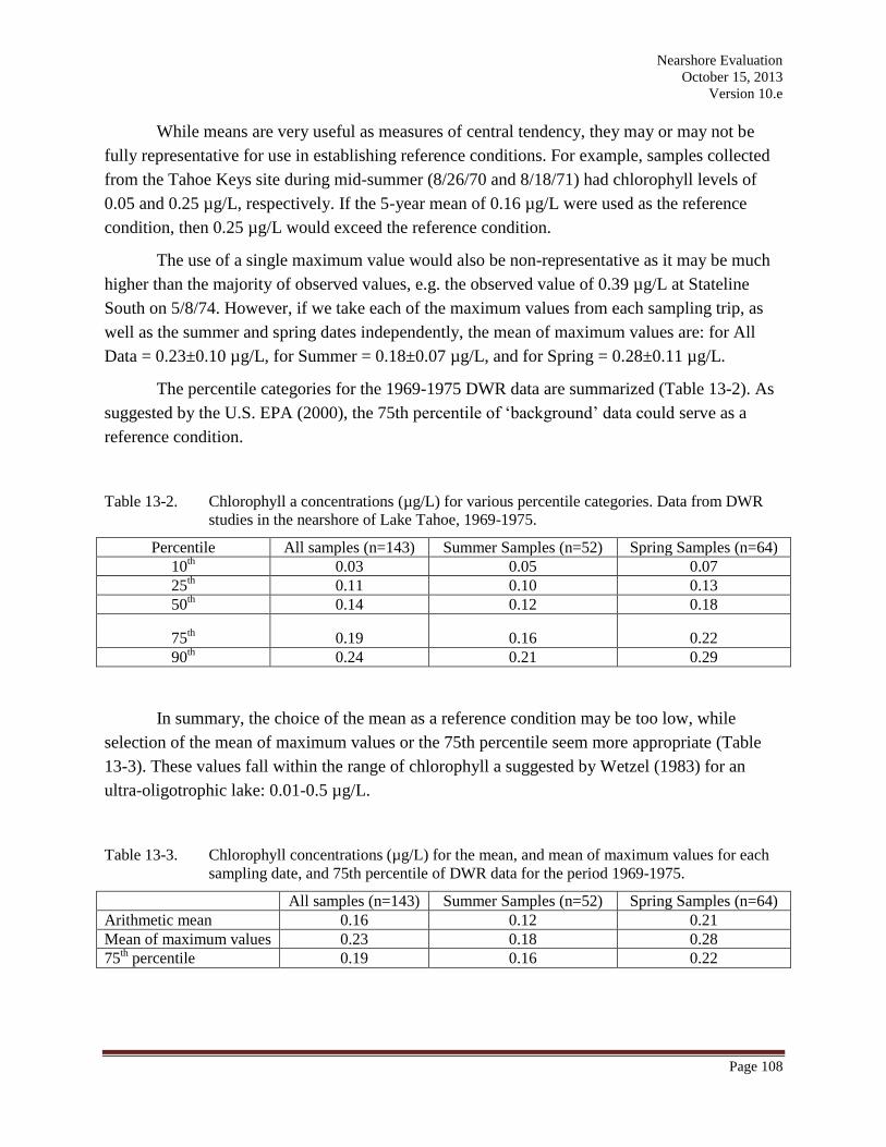
The percentile categories for the 1969-1975 DWR data are summarized (Table 13-2). As
suggested by the U.S. EPA (2000), the 75th percentile of ‘background’ data could serve as a
reference condition.
Table 13-2. Chlorophyll a concentrations (µg/L) for various percentile categories. Data from DWR
studies in the nearshore of Lake Tahoe, 1969-1975.
Percentile All samples (n=143) Summer Samples (n=52) Spring Samples (n=64)
10th 0.03 0.05 0.07
25th 0.11 0.10 0.13
50th 0.14 0.12 0.18
75th 0.19 0.16 0.22
90th 0.24 0.21 0.29
In summary, the choice of the mean as a reference condition may be too low, while
selection of the mean of maximum values or the 75th percentile seem more appropriate (Table
13-3). These values fall within the range of chlorophyll a suggested by Wetzel (1983) for an
ultra-oligotrophic lake: 0.01-0.5 µg/L.
Table 13-3. Chlorophyll concentrations (µg/L) for the mean, and mean of maximum values for each
sampling date, and 75th percentile of DWR data for the period 1969-1975.
All samples (n=143) Summer Samples (n=52) Spring Samples (n=64)
Arithmetic mean 0.16 0.12 0.21
Mean of maximum values 0.23 0.18 0.28
75th percentile 0.19 0.16 0.22
Nearshore Evaluation
October 15, 2013
Version 10.e
Page 109
We recommend that both a summer and spring reference condition be considered with
values of:
0.16-0.18 µg/L during the summer;
0.22-0.28 µg/L during the spring;
or an annual reference condition (if deemed applicable) of 0.19-0.23 µg/L.
13.3.3 Use of more recent pelagic zone data
As previously discussed, data sets for measured littoral Chl-a are largely lacking. The
exception to this are the DRI synoptic survey data, which are discussed as an independent option
below. Consequently, we tried to evaluate pelagic Chl-a and establish a relationship between
pelagic and littoral.
From 1984-2010, large and consistent changes in pelagic Chl-a have not been evident
(see Figure 13-12). The 1971-1972 study showed that the ratio of littoral to pelagic Chl-a was
1.4±0.4 (SD). If the option was selected that this relationship or ratio was itself the reference
condition, the threshold for littoral Chl-a would be 0.70-0.84 µg/L for a ratio of 1.4:1 (the
0.70-0.84 µg/L values are based on the ratio of 1.4 multiplied by the 0.50-0.60 µg/L range for
current concentrations between 2-20 m in depth). The mean of the 95th
percentile values was
somewhat higher at 1.01 µg/L.
This approach links littoral to pelagic conditions. A disadvantage is that it allows for less
protection of the littoral zone if the pelagic Chl-a rapidly increases. However, this has not been
seen since 1984. The advantage of this approach is that pelagic Chl-a straddles the boundary
between ultraoligotrophic (0.01-0.5 µg/L) and oligotrophic (0.3-3.0 µg/L)(Wetzel 2001). That is,
the pelagic concentrations are currently indicative of desired conditions for Lake Tahoe. The
ranges for ultraoligotrophic and oligotrophic represent a range for lakes worldwide. With the
implementation of the TMDL and nutrient reduction, the assumption is that pelagic Chl-a will
not greatly increase.
13.3.4 Relative chlorophyll survey approach
During full-perimeter surveys, chlorophyll a was measured in relative chlorophyll units
rather than as absolute concentrations (Fig. 13-4). Additional sample collection will be needed to
calibrate absolute chlorophyll a with relative chlorophyll values to make a reference condition
more meaningful. In the meantime, however, a spatial data analysis was conducted with existing
relative chlorophyll data to define areas that typically exhibit pristine, intermediate, or reduced
characteristics (as similarly demonstrated for turbidity and transmissivity).
Data from 1-km section polygons of applicable surveys were averaged to provide a mean
of means and the mean for coefficients of variation (CVs) within each section. This approach
Nearshore Evaluation
October 15, 2013
Version 10.e
Page 110
equally weighted the data from each survey and was not biased by the different number of
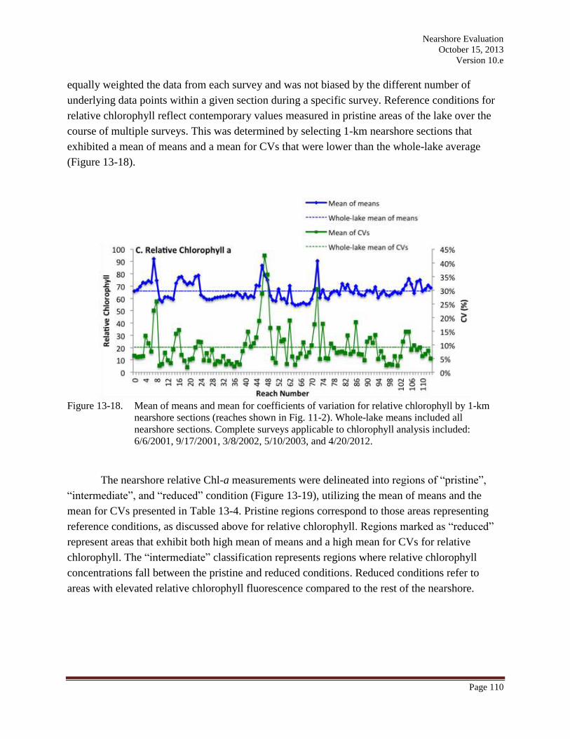
underlying data points within a given section during a specific survey. Reference conditions for
relative chlorophyll reflect contemporary values measured in pristine areas of the lake over the
course of multiple surveys. This was determined by selecting 1-km nearshore sections that
exhibited a mean of means and a mean for CVs that were lower than the whole-lake average
(Figure 13-18).
Figure 13-18. Mean of means and mean for coefficients of variation for relative chlorophyll by 1-km
nearshore sections (reaches shown in Fig. 11-2). Whole-lake means included all
nearshore sections. Complete surveys applicable to chlorophyll analysis included:
6/6/2001, 9/17/2001, 3/8/2002, 5/10/2003, and 4/20/2012.
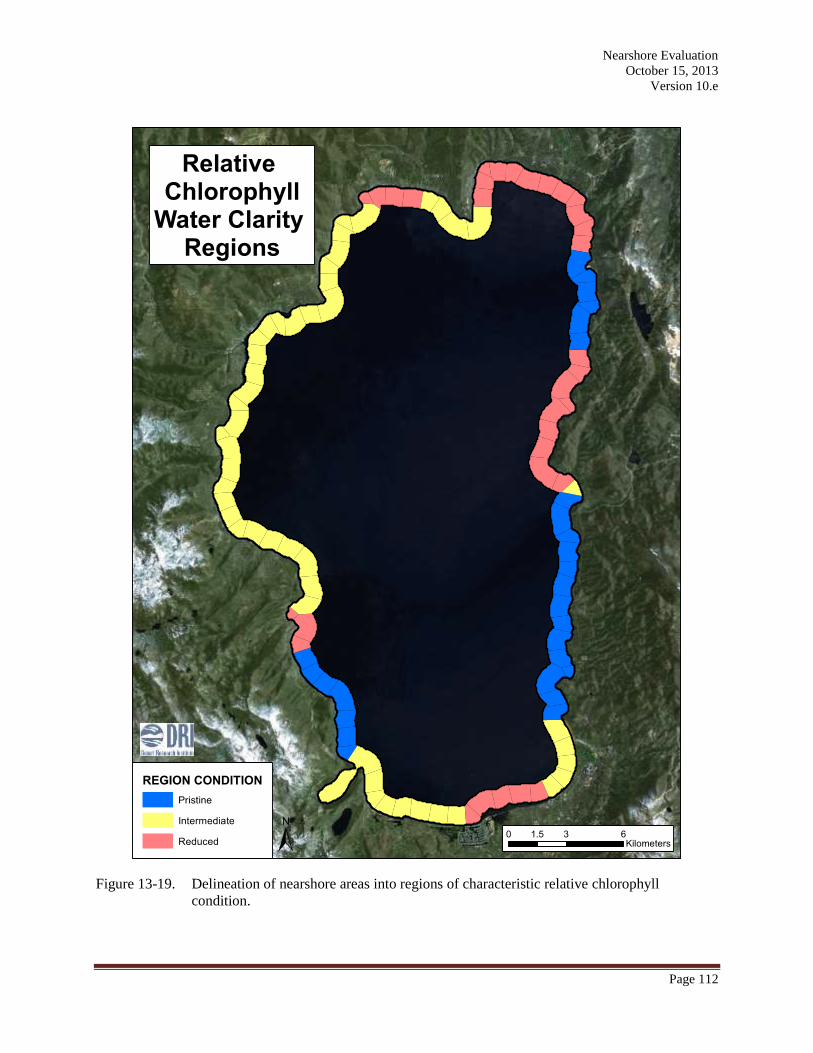
The nearshore relative Chl-a measurements were delineated into regions of “pristine”,
“intermediate”, and “reduced” condition (Figure 13-19), utilizing the mean of means and the
mean for CVs presented in Table 13-4. Pristine regions correspond to those areas representing
reference conditions, as discussed above for relative chlorophyll. Regions marked as “reduced”
represent areas that exhibit both high mean of means and a high mean for CVs for relative
chlorophyll. The “intermediate” classification represents regions where relative chlorophyll
concentrations fall between the pristine and reduced conditions. Reduced conditions refer to
areas with elevated relative chlorophyll fluorescence compared to the rest of the nearshore.
Nearshore Evaluation
October 15, 2013
Version 10.e
Page 111
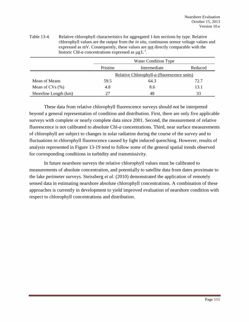
Table 13-4. Relative chlorophyll characteristics for aggregated 1-km sections by type. Relative
chlorophyll values are the output from the in situ, continuous sensor voltage values and
expressed as mV. Consequently, these values are not directly comparable with the
historic Chl-a concentrations expressed as µg.L
-1.
Water Condition Type
Pristine Intermediate Reduced
Relative Chlorophyll-a (fluorescence units)
Mean of Means 59.5 64.3 72.7
Mean of CVs (%) 4.8 8.6 13.1
Shoreline Length (km) 27 48 33
These data from relative chlorophyll fluorescence surveys should not be interpreted
beyond a general representation of condition and distribution. First, there are only five applicable
surveys with complete or nearly complete data since 2001. Second, the measurement of relative
fluorescence is not calibrated to absolute Chl-a concentrations. Third, near surface measurements
of chlorophyll are subject to changes in solar radiation during the course of the survey and to
fluctuations in chlorophyll fluorescence caused by light induced quenching. However, results of
analysis represented in Figure 13-19 tend to follow some of the general spatial trends observed
for corresponding conditions in turbidity and transmissivity.
In future nearshore surveys the relative chlorophyll values must be calibrated to
measurements of absolute concentration, and potentially to satellite data from dates proximate to
the lake perimeter surveys. Steissberg et al. (2010) demonstrated the application of remotely
sensed data in estimating nearshore absolute chlorophyll concentrations. A combination of these
approaches is currently in development to yield improved evaluation of nearshore condition with
respect to chlorophyll concentrations and distribution.
Nearshore Evaluation
October 15, 2013
Version 10.e
Page 112
Figure 13-19. Delineation of nearshore areas into regions of characteristic relative chlorophyll
condition.
Nearshore Evaluation
October 15, 2013
Version 10.e
Page 113
13.3.5 Reference Conditions for Algal Growth Potential
AGP experiments were conducted between 1969-1974 as a routine part of the California-
Nevada-Federal Joint Water Quality Investigations of Lake Tahoe (DWR 1969-1975). Eight
nearshore stations were sampled over the entire period of record with an additional six stations
cycled in and out of the monitoring program. During the first year of the testing (1969) AGP was
conducted on six individual dates. For the remainder of the years, tests were conducted in the
spring (May) and summer (August) only. Consequently we have direct data to evaluate reference
conditions for nearshore AGP. Scenarios considered include year-round conditions, spring and
summer As with our evaluation of chlorophyll a concentrations, the AGP results could be
different during other times of the year; however, that data is simply not available.
Summaries of the historic AGP ratio results are presented in Tables 13-5 through 13-7.
Each table includes information from all five years and all stations. The upper portion of these
tables shows the number and frequency of the AGP responses as the ratio of nearshore station to
the mean of both limnetic (open-water) stations). For example, if the ratio is <1.00 this means
that the AGP result was lower in the nearshore than in the open-water; a value of 1.50 denotes
that the reposnse from the nearshore station was 50 higher than the open-water, and a value of
≥2.00 shows that the nearshore response was twice that observed in the open-water. For
reference, the California water quality standard for the ratio of nearshore vs. open-water AGP in
Lake Tahoe is not to exceed a value of two. In the lower portion of the tables, a summary of the
number of times the nearshore:open-water AGP ratio exceeded a value of two is provided based
on the individual nearshore station.
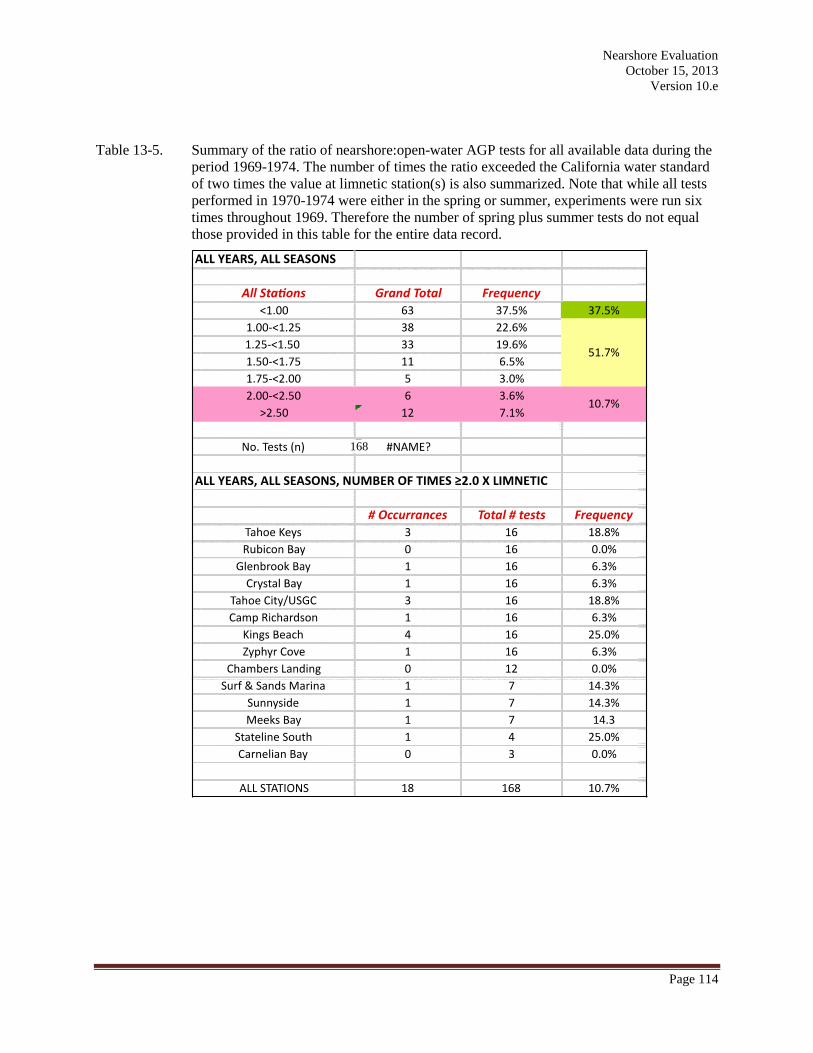
For all seasons combined during 1969-1974 the AGP response in the nearshore was less
than that in the open-water about 38 percent of the time. Approximately 50 percent of the time
the ratio was >1.00 but less than the water quality standard of 2 times the limnetic AGP. The
standard was exceeded about 11 percent of the time. Note that with the exception of Rubicon
Bay and Chambers Landing all stations had between 1-4 exceedences with a mean ±standard
deviation of 1.30±1.20. Tahoe City/USGS, Tahoe Keys and Kings Beach had the greatest
frequency of violations, among the routinely monitored stations. This may represent an early
indication of non-point source nutrient loading, but the historic data serve as the best basis for
establishing AGP reference conditions. It would be reasonable to expect an AGP ratio for
nearshore vs. pelagic of <1.5, which occurs about 80 percent of the time overall (and almost
60 percent of the time during spring season).
Nearshore Evaluation
October 15, 2013
Version 10.e
Page 114
Table 13-5. Summary of the ratio of nearshore:open-water AGP tests for all available data during the
period 1969-1974. The number of times the ratio exceeded the California water standard
of two times the value at limnetic station(s) is also summarized. Note that while all tests
performed in 1970-1974 were either in the spring or summer, experiments were run six
times throughout 1969. Therefore the number of spring plus summer tests do not equal
those provided in this table for the entire data record.
168

Nearshore Evaluation
October 15, 2013
Version 10.e
Page 115
Table 13-6. Summary of the ratio of nearshore: open-water AGP tests for test performed in the spring
(May) during the period 1969-1974. The number of times the ratio exceeded the
California water standard of two times the value at limnetic station(s) is also summarized
by nearshore station.
Nearshore Evaluation
October 15, 2013
Version 10.e
Page 116
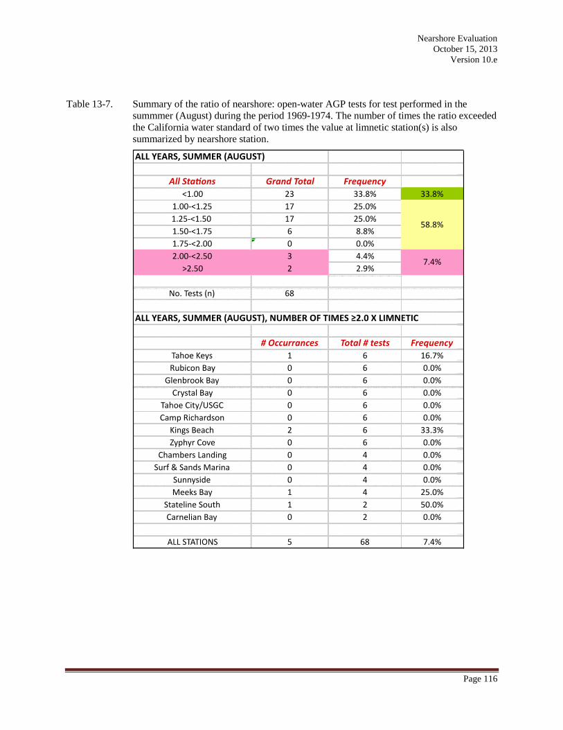
Table 13-7. Summary of the ratio of nearshore: open-water AGP tests for test performed in the
summmer (August) during the period 1969-1974. The number of times the ratio exceeded
the California water standard of two times the value at limnetic station(s) is also
summarized by nearshore station.
Nearshore Evaluation
October 15, 2013
Version 10.e
Page 117
13.4 Discussion of Threshold Values
There are currently no standards established specifically for Chl-a in the waters of Lake
Tahoe. However, both the California Lahontan Regional Water Quality Control Board and the
Nevada Division of Environmental Protection have objectives for Algal Growth Potential (AGP)
for Lake Tahoe requiring that the mean algal growth potential at any point in the lake shall not be
greater than twice the mean annual algal growth potential at the limnetic reference station. Early
water quality monitoring in Lake Tahoe, as part of the California-Nevada-Federal Joint Water
Quality Investigations program (e.g., DWR 1973), assessed nearshore algal growth potential
using Chl-a as a metric for the growth of phytoplankton biomass. These results were discussed
above. The difference between ambient Chl-a concentration and AGP lies in the term ‘potential’.
AGP measures the relative difference between pelagic and nearshore phytoplankton growth
potential, based on controlled light and temperature conditions. Chl-a on the other hand is simply
an estimate of ambient algal biomass. Many environmental factors besides nutrient level affect in
situ phytoplankton levels, including but not limited to zooplankton, protozoan and fish predation,
changes in the light environment due to lake mixing, water temperature, and high UV light levels
result in natural changes in Chl-a. These mechanisms are not accounted for in AGP experiments
and may lead to misinterpretations regarding ambient conditions (Hecky and Kilham, 1988).
Suspended Chl-a provides a convenient and accepted metric for measuring phytoplankton
biomass, while AGP provides a useful assessment of the aggregate phytoplankton response to
variable conditions associated with nutrient and species interactions.
Recommendations at this time for nearshore chlorophyll thresholds would be premature,
as the interpretation would be based on diverse and relatively sparse datasets. There must be a
concerted effort to establish a reliable base set of high quality data with calibrations between
relative chlorophyll measurements by fluorometer and absolute Chl-a measured by analytic
chemistry methods. Other technical issues also must be resolved. In the meantime these results
should be viewed as interim evaluations that would be reviewed after additional data collection
as part of a coordinated monitoring program.
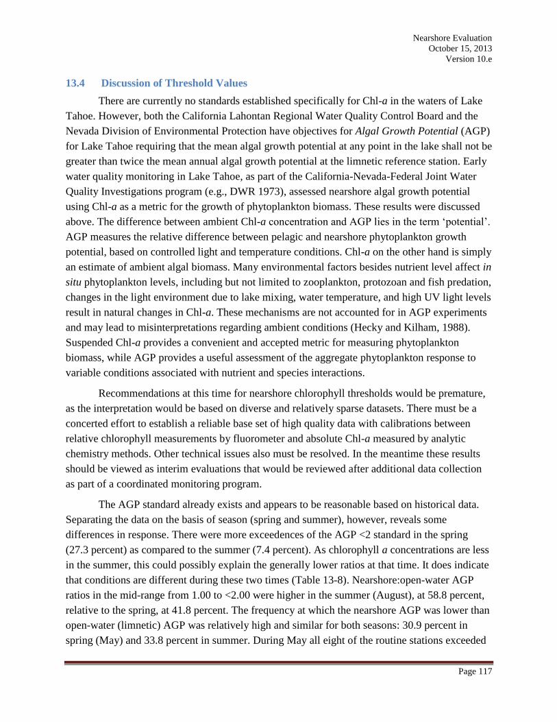
The AGP standard already exists and appears to be reasonable based on historical data.
Separating the data on the basis of season (spring and summer), however, reveals some
differences in response. There were more exceedences of the AGP <2 standard in the spring
(27.3 percent) as compared to the summer (7.4 percent). As chlorophyll a concentrations are less
in the summer, this could possibly explain the generally lower ratios at that time. It does indicate
that conditions are different during these two times (Table 13-8). Nearshore:open-water AGP
ratios in the mid-range from 1.00 to <2.00 were higher in the summer (August), at 58.8 percent,
relative to the spring, at 41.8 percent. The frequency at which the nearshore AGP was lower than
open-water (limnetic) AGP was relatively high and similar for both seasons: 30.9 percent in
spring (May) and 33.8 percent in summer. During May all eight of the routine stations exceeded
Nearshore Evaluation
October 15, 2013
Version 10.e
Page 118
the water quality standard on 1-3 occasions of the five sampling dates. During August only
Tahoe Keys, Kings Beach, Stateline South, and Meeks Bay exceeded the standard. This suggests
that existing standards or new thresholds might wish to consider both seasonal and locational
differences if updated to reflect contemporary data (currently in development) relative to
historical conditions. Exceedance criteria may also need to be specified.
Table 13-8. Summary of conditions on a whole-lake basis for the ratio of nearshore:open-water AGP,
based on actual field conditions during the period 1969-1974. Data were aggregated from
Tables 13-5 through 13-7 as derived from DWR (1969-1974) reports.
13.5 Metric Monitoring Plan
No standard currently exists for nearshore chlorophyll in Lake Tahoe. Therefore, it is
imperative to establish a monitoring program that would collect the data needed to more fully
evaluate existing conditions, its variability, and the relationships to other metrics and indicators.
Winder and Reuter (2009) developed an extensive monitoring protocol for Chl-a. This should be
combined with a routine of full-perimeter nearshore surveys for turbidity, transmissivity, and
chlorophyll. However, these methods are still in development and improved techniques will be
required to overcome inherent bias and artifacts due to issues like differential solar quenching of
Chl-a in the near-surface waters.
In the meantime, we recommend a set of depth profiles distributed around the nearshore
during perimeter cruises, associated with phytoplankton collections. These depth profiles should
include discrete samples taken for absolute Chl-a measurements and AGP, as well as continuous
down-cast measurements for relative Chl-a, transmissivity and turbidity. Measurements would
be collected by an array of sensors that include a chlorophyll fluorometer (WetLabs WetStar),
Nearshore Evaluation
October 15, 2013
Version 10.e
Page 119
with data passed to CR1000 dataloggers for computer processing, storage, and real-time display
in conjunction with data from the GPS receiver.
Following manufacturer instructions the fluorometer is calibrated prior to each run by
filling the chamber cuvette with flat (non-carbonated) coca-cola to establish the “zero” range and
then using an empty chamber to establish the “full” range. External calibrations will also be
conducted on each run by collecting water samples from the flow line after passing through the
sensor chamber and submitting to analytic chlorophyll analysis using Standard Methods (2005).
As with turbidity and transmissivity, these surveys are expected to typically require 2 to 3
days for completion and should follow the same path each time. We recommend at least four
sampling periods per year, on a seasonal basis, with 3 to 9 depth profiles distributed around the
lake perimeter. More frequent sampling may be required initially to establish a robust dataset for
calibration. This is an important metric, and is currently an area of active research, but the
approach, methods and technology may change substantially as existing issues associated with
obtaining reliable high-quality are resolved.
14.0 NEARSHORE PHYTOPLANKTON
The free-floating algae in lakes are referred to as phytoplankton. These organisms
typically form the base of the aquatic food web as they use sunlight, carbon dioxide and nutrients
to create organic biomass. In a simple food chain, these organisms are consumed by
zooplankton, and in turn by higher order invertebrates and fish. Phytoplankton can also be part of
the microbial food loop which includes dissolved organic carbon, bacteria and the entire
microbial food web, protozoans and other microzooplankton. When present in too high a level
phytoplankton degrade water quality and drive cultural eutrophication.
Phytoplankton consists of diverse assemblage of many different major taxonomic groups,
including, but not limited to diatoms, green algae, cryptophytes, chyrsophytes, dinoflagellates,
euglenoids and blue-green algae (cyanobacteria). These groups, and the individual species with
each group, have different pigments, morphological characteristics, resource requirements,
growth rates and sinking velocities (e.g. Reynolds 2006). Their size can range over several
several orders of magnitude (~0.2-200 µm).
Hutchinson (1961) raised the issue of what he called the “paradox of the plankton”. This
refers to the fact that many tens of phytoplankton species can coexist in lake water. A foundation
of ecological competition theory holds that if two organisms compete for resource one will win
out over the other. If so, Hutchinson postulated that phytoplankton were able to achieve niche
separation based on naturally occurring gradients of light, nutrient and water movement;
differential predation; combinations of all or some of these factors; and an otherwise constantly
changing environment. This is important as it explains why so many species are present, and
why species change as trophic status or other conditions change. This has allowed scientists to
Nearshore Evaluation
October 15, 2013
Version 10.e
Page 120
classify phytoplankton species composition on the basis of trophic state and other lake
characteristics.
As lake conditions change over the course of a year, the phytoplankton community will
experience seasonal succession (EPA 1988). This phenomenon will generally repeat itself
between years provided there are no major environmental changes. These seasonal differences
are a natural occurrence and are not particularly useful as indicators of water quality or changing
trophic status. However, based on numerous, world-wide observational studies of lake
phytoplankton some general conclusions can be made with regard to species composition and
trophic status (e.g., Eloranta 1986, Wetzel 1983, Reynolds 2006, Hunter TERC unpub. data).
In general, ultra-oligotrophic and oligotrophic lakes contain diatoms, chrysophytes and
dinoflagellates, with diatom dominance. However, it is important to emphasize that all the
individual species that make up these larger taxonomic groups are found in only oligotrophic
conditions. Select species in all these groups are found in water across the entire trophic status
spectrum. As trophic status moves away from oligtrophy and reaches eutrophy other groups
become more prevalent, e.g. cyanobacteria, euglenoids, green algae and different species of
diatoms. Species composition is very important in the food web and for the productivity of the
grazers and consumers. Diatoms contain relatively large amounts of highly unsaturated fatty
acids, a material with very high food quality. Certain species of cyanobacteria, in eutrophic
bloom conditions can create nuisance conditions, release toxins and are create taste and odor
problems, and are therefore quite undesirable.
14.1 History of Metric Monitoring
The DWR monitoring from 1969–1974 did make a cursory analysis of nearshore
phytoplankton species. However, the methodology used in those studies employed the
Sedgewick-Rafter counting strip at 200x magnification. This is less effective than current
methods at capturing very small cells that are important to the phytoplankton community.
Therefore, the early DWR data are not entirely representative or comparable to more recent data.
By far, the most comprehensive and detailed study of phytoplankton taxonomy and
enumeration conducted in the nearshore of Lake Tahoe was done by Eloranta and Loeb (1984),
and Loeb (1983). While there were some isolated studies of samples taken for nearshore
phytoplankton in the past, as mentioned above, none have the breath of subsequent work by
Loeb et al. Unfortunately, these data from 1981-1982 are over 30 years old with no comparable
data collected since.
The overall goal of that study was to document seasonal and spatial trends in water
quality and phytoplankton productivity in the littoral zone of Lake Tahoe. It was intended that
this data would be supportive of the sewer-line exfiltration investigations that were active at that
Nearshore Evaluation
October 15, 2013
Version 10.e
Page 121
time, early urban runoff studies, and the then new Lake Tahoe Interagency Monitoring Program
measuring stream flow and nutrient loading (Loeb 1983).
Sampling sites included Sunnyside-Pineland, Rubicon Point, Zeyphr Point and the six
stations along the south shore (Baldwin Beach - SS-1; Kiva Beach – SS-2; Tahoe Keys western
channel – SS-3; Reagan Beach – SS-4; Wildwood Avenue – SS-5; and Stateline east – SS-6).
Each station was in the shallows waters of the littoral zone at a maximum depth of 2-3 m. Water
was collected at an intermediate depth. Phytoplankton was collected monthly between July 1981
and July 1982, except for the period October-February when sampling was every other month.
14.2 Monitoring Data Summary
A total of ca. 380 algal taxa were recorded in 128 littoral phytoplankton samples during
the UC Davis study. Diatoms accounted for 36 percent of the total number of species with
approximately three-quarters of these being benthic forms. Besides diatoms, the green algae and
chrysophytes were also rich in number contributing 86 and 50 species, respectively (Eloranta and
Loeb 1984).
Generally, the major taxonomic groups that dominated littoral zone phytoplankton were
found to be similar to those found in the pelagic waters (Loeb, 1983). In particular, this was the
case for the major biomass dominants. For example, Monoraphidium contortum and
Rhodomonas lacustris were co-dominant in both regions from February to April along with
several species of Cyclotella. However, Chromulina sp. and Synura radians, while dominants in
the summer nearshore community were not found in large abundance in the open waters.
Of all the study sites, the south shore stations had the highest species diversity (Loeb
1983). In addition, that study found that three groups which are most indicative of lake water
fertility (green algae, cyanophytes and euglenoids) were more abundant at the south shore versus
the other stations. SS-3, located 50 m off the western channel of the Tahoe Keys Marina
consistently had the highest diversity of phytoplankton.
The occurrence of cyanophytes and euglenoids are extremely rare in the pelagic waters of
Lake Tahoe, however, they were not uncommon in the littoral phytoplankton. The genus
Anabaena, a species found in waters of higher fertility (nutrient concentrations), was found at all
of the south shore stations on several sampling dates. The genera Oscillatoria, Lyngbya,
Chrococcus and Aphanocapsa were also present. Cyanophytes were not found at the other three
stations with the exception of once at Rubicon and only accounted for 0.05 - 0.30 percent of the
total biomass at each of the nine stations.
Euglenoids were seen on only one date each at Pineland-Sunnyside and Rubicon, and on
two dates at Zephyr Point. All six south shore sites had from two (SS-5) to eight (SS-3)
occurrences.
Nearshore Evaluation
October 15, 2013
Version 10.e
Page 122
Green algae or chlorophytes, were consistently more diverse along the south shore.
Mean monthly phytoplankton biomass at all stations combined ranged from
approximately 20 to 100 mg/m3 (Eloranta and Loeb 1984) with the highest mean biomass (90-
100 mg/m3) in May-June and an annual mean of 43.6±5.7 mg/m
3 (±SD). The mean±SD for the
three stations not along the south shore was 38.1±5.2 mg/m3. The mean±SD for the six south
shore stations was 44.4±6.2 mg/m3. There was no real difference between these two sets of
stations. The minimum biomass on any single date from any station was 9 mg/m3 (Rubicon
Point) while the maximum single value was 174 mg/m3 (Sunnyside-Pineland). The contribution
of the major taxonomic groups to total community biomass were on the order of: diatoms - 40
percent, chrysophytes - 20 percent, dinoflagellates - 20 percent, chlorophyes - 15-20 percent
and cryptophytes - 10 percent. Elevated diatom biomass was found in February-June (spring-
early summer), while periods of peak biomass for the other groups were, dinoflagellates –
July-October (summer), crytophyes – December-April (winter), chrysophytes – July-December
(summer and fall), and chlorophytes – October-April (late fall and winter (Eloranta and Loeb
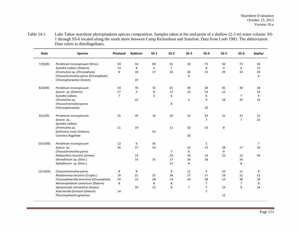
1984). The important individual contributors to nearshore biomass are summarized in
Table 14-1.
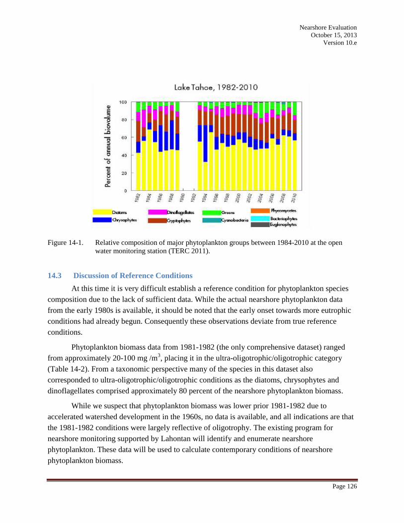
In comparison, the percent composition of the major taxonomic groups in the pelagic
waters from 1982-2010 is shown in Figure 14-1 (TERC 2011). The contribution of chyrsophytes
and dinoflagellates was 5-10 and 10 percent higher, respectively, during 1982 in the nearshore
versus open water. Cryptophytes were 10-15 percent lower in the nearshore. Despite this
differences, the distribution of the major taxonomic groups were very similar between the
nearshore and the open water in 1982. While there have been some changes in the percent
composition in the open water phytoplankton over the years, the major taxonomic groups and the
relative composition remain similar Figure 14-1.
In 2010 (TERC 2011), open water phytoplankton biomass ranged from approximately
45-210 mg/m3 with an annual mean on the order of 90-100 mg/m
3.
Nearshore Evaluation
October 15, 2013
Version 10.e
Page 123
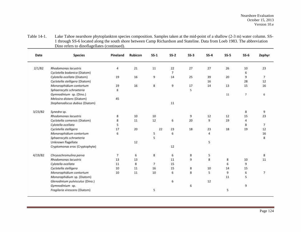
Table 14-1. Lake Tahoe nearshore phytoplankton species composition. Samples taken at the mid-point of a shallow (2-3 m) water column. SS-
1 through SS-6 located along the south shore between Camp Richardson and Stateline. Data from Loeb 1983. The abbreviation
Dino refers to dinoflagellates.
Nearshore Evaluation
October 15, 2013
Version 10.e
Page 124
Table 14-1. Lake Tahoe nearshore phytoplankton species composition. Samples taken at the mid-point of a shallow (2-3 m) water column. SS-
1 through SS-6 located along the south shore between Camp Richardson and Stateline. Data from Loeb 1983. The abbreviation
Dino refers to dinoflagellates (continued).
Nearshore Evaluation
October 15, 2013
Version 10.e
Page 125
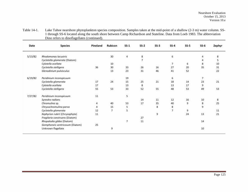
Table 14-1. Lake Tahoe nearshore phytoplankton species composition. Samples taken at the mid-point of a shallow (2-3 m) water column. SS-
1 through SS-6 located along the south shore between Camp Richardson and Stateline. Data from Loeb 1983. The abbreviation
Dino refers to dinoflagellates (continued).
Nearshore Evaluation
October 15, 2013
Version 10.e
Page 126
Figure 14-1. Relative composition of major phytoplankton groups between 1984-2010 at the open
water monitoring station (TERC 2011).
14.3 Discussion of Reference Conditions
At this time it is very difficult establish a reference condition for phytoplankton species
composition due to the lack of sufficient data. While the actual nearshore phytoplankton data
from the early 1980s is available, it should be noted that the early onset towards more eutrophic
conditions had already begun. Consequently these observations deviate from true reference
conditions.
Phytoplankton biomass data from 1981-1982 (the only comprehensive dataset) ranged
from approximately 20-100 mg /m3, placing it in the ultra-oligotrophic/oligotrophic category
(Table 14-2). From a taxonomic perspective many of the species in this dataset also
corresponded to ultra-oligotrophic/oligotrophic conditions as the diatoms, chrysophytes and
dinoflagellates comprised approximately 80 percent of the nearshore phytoplankton biomass.
While we suspect that phytoplankton biomass was lower prior 1981-1982 due to
accelerated watershed development in the 1960s, no data is available, and all indications are that
the 1981-1982 conditions were largely reflective of oligotrophy. The existing program for
nearshore monitoring supported by Lahontan will identify and enumerate nearshore
phytoplankton. These data will be used to calculate contemporary conditions of nearshore
phytoplankton biomass.
Nearshore Evaluation
October 15, 2013
Version 10.e
Page 127
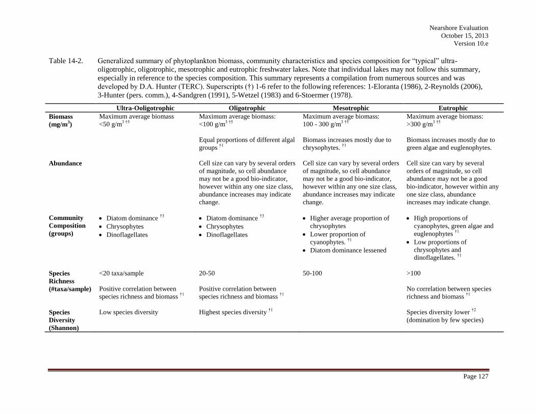
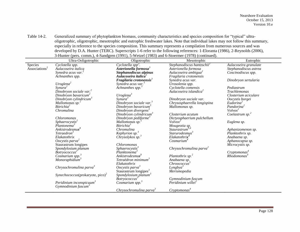
Table 14-2. Generalized summary of phytoplankton biomass, community characteristics and species composition for “typical” ultra-
oligotrophic, oligotrophic, mesotrophic and eutrophic freshwater lakes. Note that individual lakes may not follow this summary,
especially in reference to the species composition. This summary represents a compilation from numerous sources and was
developed by D.A. Hunter (TERC). Superscripts (†) 1-6 refer to the following references: 1-Eloranta (1986), 2-Reynolds (2006),
3-Hunter (pers. comm.), 4-Sandgren (1991), 5-Wetzel (1983) and 6-Stoermer (1978).
Ultra-Ooligotrophic Oligotrophic Mesotrophic Eutrophic
Biomass
(mg/m3)
Maximum average biomass
<50 g/m3 †5
Maximum average biomass:
<100 g/m3 †5
Equal proportions of different algal
groups †1
Maximum average biomass:
100 - 300 g/m3 †5
Biomass increases mostly due to
chrysophytes. †1
Maximum average biomass:
>300 g/m3 †5
Biomass increases mostly due to
green algae and euglenophytes.
Abundance Cell size can vary by several orders
of magnitude, so cell abundance
may not be a good bio-indicator,
however within any one size class,
abundance increases may indicate
change.
Cell size can vary by several orders
of magnitude, so cell abundance
may not be a good bio-indicator,
however within any one size class,
abundance increases may indicate
change.
Cell size can vary by several
orders of magnitude, so cell
abundance may not be a good
bio-indicator, however within any
one size class, abundance
increases may indicate change.
Community
Composition
(groups)
Diatom dominance †3
Chrysophytes
Dinoflagellates
Diatom dominance †3
Chrysophytes
Dinoflagellates
Higher average proportion of
chrysophytes
Lower proportion of
cyanophytes. †1
Diatom dominance lessened
High proportions of
cyanophytes, green algae and
euglenophytes †1
Low proportions of
chrysophytes and
dinoflagellates. †1
Species
Richness
(#taxa/sample)
<20 taxa/sample
Positive correlation between
species richness and biomass †1
20-50
Positive correlation between
species richness and biomass †1
50-100 >100
No correlation between species
richness and biomass †1
Species
Diversity
(Shannon)
Low species diversity
Highest species diversity †1
Species diversity lower †2
(domination by few species)
Nearshore Evaluation
October 15, 2013
Version 10.e
Page 128
Table 14-2. Generalized summary of phytoplankton biomass, community characteristics and species composition for “typical” ultra-
oligotrophic, oligotrophic, mesotrophic and eutrophic freshwater lakes. Note that individual lakes may not follow this summary,
especially in reference to the species composition. This summary represents a compilation from numerous sources and was
developed by D.A. Hunter (TERC). Superscripts 1-6 refer to the following references: 1-Eloranta (1986), 2-Reynolds (2006),
3-Hunter (pers. comm.), 4-Sandgren (1991), 5-Wetzel (1983) and 6-Stoermer (1978) (continued).
Ultra-Ooligotrophic Oligotrophic Mesotrophic Eutrophic
Species Associations
2
Cyclotella spp. Aulacoseira italica Synedra acus var.
2
Achnanthes spp.
Uroglena2
Synura2
Dinobryon sociale var.2
Dinobryon bavaricum2
Dinobryon cylindricum3
Mallomonas sp.2
Bitrichia2
Chromulina
Chloromonas Sphaerocystis
2
Plantonema3
Ankistrodesmus3
Tetraedron3
Elakatothrix Oocystis parva
2
Staurastrum longipes Spondylosium planum Botryococcus
2
Cosmarium spp.3
Monoraphidium3
Chrysochromulina parva3
Synechococcus(prokaryote, pico)2
Peridinium inconspicuum3
Gymnodinium fuscum3
Cyclotella spp3.
Asterionella formosa3
Stephanodiscus alpinus Aulacoseira italica
3
Fragilaria crotonensis3
Synedra acus var.3
Achnanthes spp.3
Uroglena3
Synura3
Dinobryon sociale var.3
Dinobryon bavaricum3
Dinobryon divergens3
Dinobryon cylindricum3
Dinobryon pediforme3
Mallomonas sp.2
Bitrichia3
Chromulina Kephyrion sp.
3
Chrysolykos sp.3
Chloromonas Sphaerocystis
3
Planktonema3
Ankistrodesmus3
Tetraëdron minimum3
Elakatothrix Oocystis parva
3
Staurastrum longipes3
Spondylosium planum3
Botryococcus3
Cosmarium spp.3
Chrysochromulina parva3
Stephanodiscus hantzschii2
Asterionella formosa Aulacoseira ambigua
2
Fragilaria crotonensis Synedra acus var. Urosolenia spp. Cyclotella comensis Aulacoseira islandica
2
Dinobryon sociale var. Chrysosphaerella longispina Mallomonas sp.
Closterium acutum Dictyosphaerium pulchellum Volvox
2
Mougeotia sp. Staurastrum
3,4
Starurodesmus3
Elakatothrix3
Cosmarium4
Chrysochromulina parva2
Plantothrix sp.2
Anabaena sp. Chroococcus
3
Lyngbya3
Merismopedia
Gymnodinium fuscum Peridinium willei
2
Cryptomonas4
Aulacoseira granulate Stephanodiscus astrea Coscinodiscus spp.
Dinobryon sertularia
Pediastrum Trachlemonas Closterium aciculare Oocystis borgei Eudorina
2
Pandorina2
Volvox2
Coelastrum sp.2
Euglena sp.
Aphanizomenon sp. Planktothrix sp. Anabaena sp. Aphanocapsa sp. Microcystis sp.
Cryptomonas4
Rhodomonas4
Nearshore Evaluation
October 15, 2013
Version 10.e
Page 129
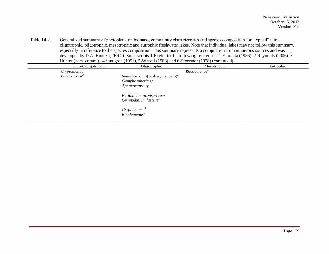
Table 14-2. Generalized summary of phytoplankton biomass, community characteristics and species composition for “typical” ultra-
oligotrophic, oligotrophic, mesotrophic and eutrophic freshwater lakes. Note that individual lakes may not follow this summary,
especially in reference to the species composition. This summary represents a compilation from numerous sources and was
developed by D.A. Hunter (TERC). Superscripts 1-6 refer to the following references: 1-Eloranta (1986), 2-Reynolds (2006), 3-
Hunter (pers. comm.), 4-Sandgren (1991), 5-Wetzel (1983) and 6-Stoermer (1978) (continued).
Ultra-Ooligotrophic Oligotrophic Mesotrophic Eutrophic
Cryptomonas3
Rhodomonas3
Synechococcus(prokaryote, pico)2
Gomphospheria sp.
Aphanocapsa sp.
Peridinium inconspicuum3
Gymnodinium fuscum3
Cryptomonas3
Rhodomonas3
Rhodomonas4
Nearshore Evaluation
October 15, 2013
Version 10.e
Page 130
14.4 Recommendations of Thresholds Values
We do not recommend that phytoplankton biovolume/biomass be used as a threshold.
This is a very time consuming analysis and chlorophyll is very commonly used as a surrogate
measurement. Neither do we believe that species richness or species diversity make good
thresholds. Both these measures of phytoplankton biodiversity can be quite variable, and not
reliable enough to use as numeric thresholds.
The goal of setting a threshold for phytoplankton species composition should be to
identify when individual species, not characteristic of oligotrophy and more characteristic of
meso- and eutrophy are observed. We recommend that this metric not be used in the strict sense
of a numeric threshold, i.e. exceedance of a specified value. Rather, phytoplankton species
composition should focus on changes both at the community and individual species scales. For
example, a trend away from a dominance by diatoms with a higher average proportion of
chrysophytes or increase in the proportion of cyanophytes can be taken as a possible “red-flag”,
requiring further inquiry. Refer to Table 8-2 for more information on species composition that
could indicate a change in trophic status based on phytoplankton.
14.5 Metric Monitoring Plan
For analysis of changes in community composition and individual taxa, samples should
be taken a series of 9 sites around the lake corresponding to various levels of watershed
development. While more discussion will be needed to finalize these sites, a possible set of
stations includes, Rubicon Point, Meeks Bay, Tahoe City, Kings Beach, Glenbrook, Zeyphr
Cove, Stateline south, off Tahoe Keys and Kiva Beach. Since the objective is to identify a high
abundance of unwanted species, two sampling dates should be selected; both during the summer
when public use of the nearshore is maximum.
To determine the species associated with high levels of phytoplankton (to determine if
potential bloom-forming organisms are in abundance) samples would be collected and analyzed
only when real-time chlorophyll concentrations exceeded a value of ~5 mg/m3 during these
perimeter surveys. Based on early sampling results, the chlorophyll value that triggers
phytoplankton sampling will be re-evaluated. Sampling would be taken from the same depth as
the real-time chlorophyll measurements and collected using the same water pumping system.
Phytoplankton samples would be preserved and enumerated according to the methods used by
LTIMP for Lake Tahoe water (Winder and Hunter 2008).
Nearshore Evaluation
October 15, 2013
Version 10.e
Page 131
15.0 PERIPHYTON
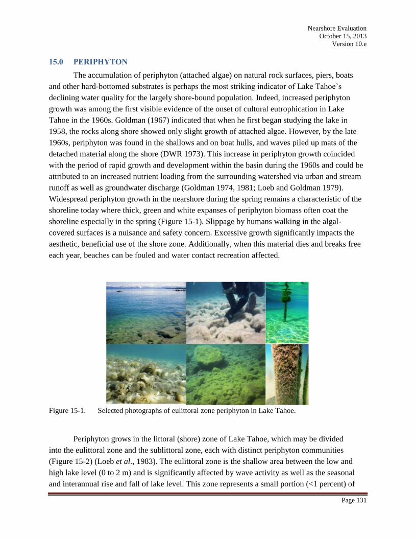
The accumulation of periphyton (attached algae) on natural rock surfaces, piers, boats
and other hard-bottomed substrates is perhaps the most striking indicator of Lake Tahoe’s
declining water quality for the largely shore-bound population. Indeed, increased periphyton
growth was among the first visible evidence of the onset of cultural eutrophication in Lake
Tahoe in the 1960s. Goldman (1967) indicated that when he first began studying the lake in
1958, the rocks along shore showed only slight growth of attached algae. However, by the late
1960s, periphyton was found in the shallows and on boat hulls, and waves piled up mats of the
detached material along the shore (DWR 1973). This increase in periphyton growth coincided
with the period of rapid growth and development within the basin during the 1960s and could be
attributed to an increased nutrient loading from the surrounding watershed via urban and stream
runoff as well as groundwater discharge (Goldman 1974, 1981; Loeb and Goldman 1979).
Widespread periphyton growth in the nearshore during the spring remains a characteristic of the
shoreline today where thick, green and white expanses of periphyton biomass often coat the
shoreline especially in the spring (Figure 15-1). Slippage by humans walking in the algal-
covered surfaces is a nuisance and safety concern. Excessive growth significantly impacts the
aesthetic, beneficial use of the shore zone. Additionally, when this material dies and breaks free
each year, beaches can be fouled and water contact recreation affected.
Figure 15-1. Selected photographs of eulittoral zone periphyton in Lake Tahoe.
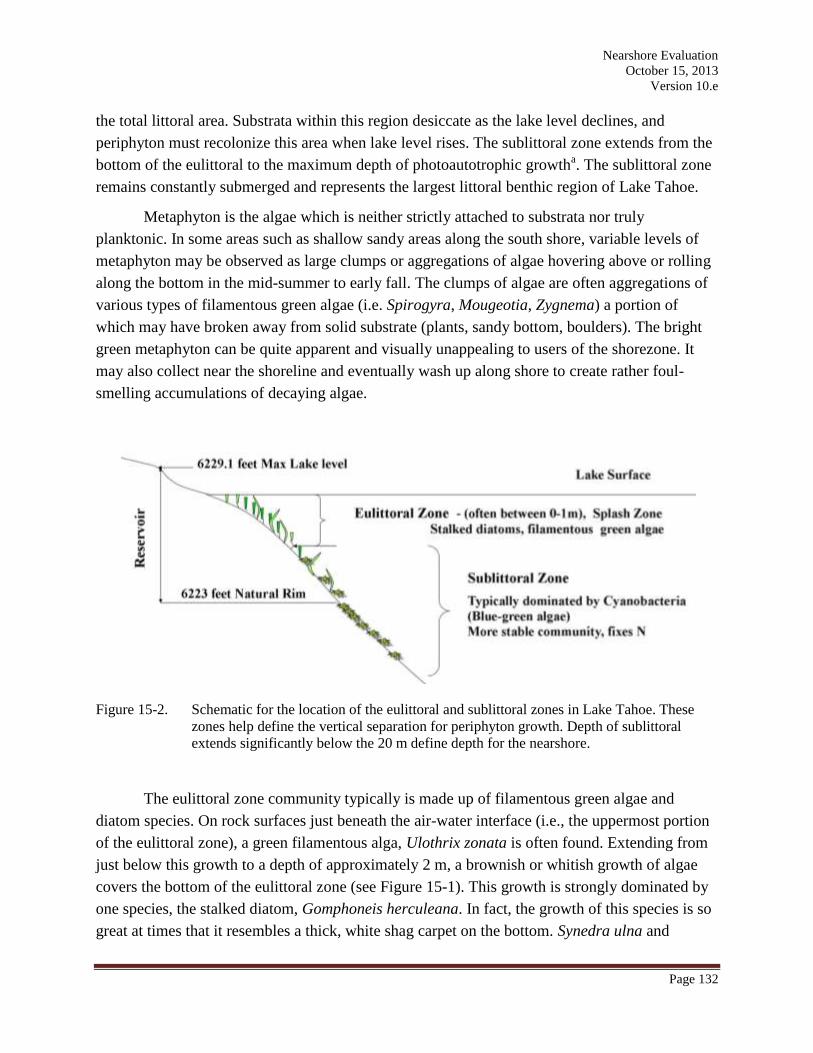
Periphyton grows in the littoral (shore) zone of Lake Tahoe, which may be divided
into the eulittoral zone and the sublittoral zone, each with distinct periphyton communities
(Figure 15-2) (Loeb et al., 1983). The eulittoral zone is the shallow area between the low and
high lake level (0 to 2 m) and is significantly affected by wave activity as well as the seasonal
and interannual rise and fall of lake level. This zone represents a small portion (<1 percent) of
Nearshore Evaluation
October 15, 2013
Version 10.e
Page 132
the total littoral area. Substrata within this region desiccate as the lake level declines, and
periphyton must recolonize this area when lake level rises. The sublittoral zone extends from the
bottom of the eulittoral to the maximum depth of photoautotrophic growtha. The sublittoral zone
remains constantly submerged and represents the largest littoral benthic region of Lake Tahoe.
Metaphyton is the algae which is neither strictly attached to substrata nor truly
planktonic. In some areas such as shallow sandy areas along the south shore, variable levels of
metaphyton may be observed as large clumps or aggregations of algae hovering above or rolling
along the bottom in the mid-summer to early fall. The clumps of algae are often aggregations of
various types of filamentous green algae (i.e. Spirogyra, Mougeotia, Zygnema) a portion of
which may have broken away from solid substrate (plants, sandy bottom, boulders). The bright
green metaphyton can be quite apparent and visually unappealing to users of the shorezone. It
may also collect near the shoreline and eventually wash up along shore to create rather foul-
smelling accumulations of decaying algae.
Figure 15-2. Schematic for the location of the eulittoral and sublittoral zones in Lake Tahoe. These
zones help define the vertical separation for periphyton growth. Depth of sublittoral
extends significantly below the 20 m define depth for the nearshore.
The eulittoral zone community typically is made up of filamentous green algae and
diatom species. On rock surfaces just beneath the air-water interface (i.e., the uppermost portion
of the eulittoral zone), a green filamentous alga, Ulothrix zonata is often found. Extending from
just below this growth to a depth of approximately 2 m, a brownish or whitish growth of algae
covers the bottom of the eulittoral zone (see Figure 15-1). This growth is strongly dominated by
one species, the stalked diatom, Gomphoneis herculeana. In fact, the growth of this species is so
great at times that it resembles a thick, white shag carpet on the bottom. Synedra ulna and
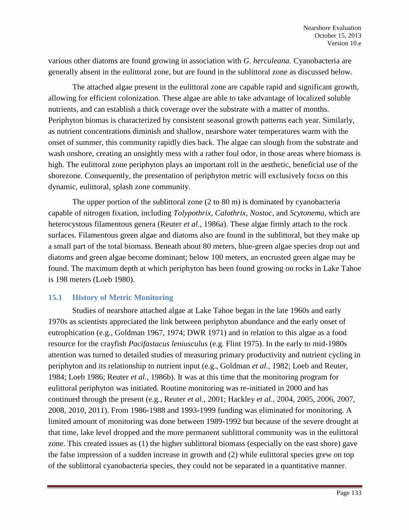
Nearshore Evaluation
October 15, 2013
Version 10.e
Page 133
various other diatoms are found growing in association with G. herculeana. Cyanobacteria are
generally absent in the eulittoral zone, but are found in the sublittoral zone as discussed below.
The attached algae present in the eulittoral zone are capable rapid and significant growth,
allowing for efficient colonization. These algae are able to take advantage of localized soluble
nutrients, and can establish a thick coverage over the substrate with a matter of months.
Periphyton biomas is characterized by consistent seasonal growth patterns each year. Similarly,
as nutrient concentrations diminish and shallow, nearshore water temperatures warm with the
onset of summer, this community rapidly dies back. The algae can slough from the substrate and
wash onshore, creating an unsightly mess with a rather foul odor, in those areas where biomass is
high. The eulittoral zone periphyton plays an important roll in the aesthetic, beneficial use of the
shorezone. Consequently, the presentation of periphyton metric will exclusively focus on this
dynamic, eulittoral, splash zone community.
The upper portion of the sublittoral zone (2 to 80 m) is dominated by cyanobacteria
capable of nitrogen fixation, including Tolypothrix, Calothrix, Nostoc, and Scytonema, which are
heterocystous filamentous genera (Reuter et al., 1986a). These algae firmly attach to the rock
surfaces. Filamentous green algae and diatoms also are found in the sublittoral, but they make up
a small part of the total biomass. Beneath about 80 meters, blue-green algae species drop out and
diatoms and green algae become dominant; below 100 meters, an encrusted green algae may be
found. The maximum depth at which periphyton has been found growing on rocks in Lake Tahoe
is 198 meters (Loeb 1980).
15.1 History of Metric Monitoring
Studies of nearshore attached algae at Lake Tahoe began in the late 1960s and early
1970s as scientists appreciated the link between periphyton abundance and the early onset of
eutrophication (e.g., Goldman 1967, 1974; DWR 1971) and in relation to this algae as a food
resource for the crayfish Pacifastacus leniusculus (e.g. Flint 1975). In the early to mid-1980s
attention was turned to detailed studies of measuring primary productivity and nutrient cycling in
periphyton and its relationship to nutrient input (e.g., Goldman et al., 1982; Loeb and Reuter,
1984; Loeb 1986; Reuter et al., 1986b). It was at this time that the monitoring program for
eulittoral periphyton was initiated. Routine monitoring was re-initiated in 2000 and has
continued through the present (e.g., Reuter et al., 2001; Hackley et al., 2004, 2005, 2006, 2007,
2008, 2010, 2011). From 1986-1988 and 1993-1999 funding was eliminated for monitoring. A
limited amount of monitoring was done between 1989-1992 but because of the severe drought at
that time, lake level dropped and the more permanent sublittoral community was in the eulittoral
zone. This created issues as (1) the higher sublittoral biomass (especially on the east shore) gave
the false impression of a sudden increase in growth and (2) while eulittoral species grew on top
of the sublittoral cyanobacteria species, they could not be separated in a quantitative manner.
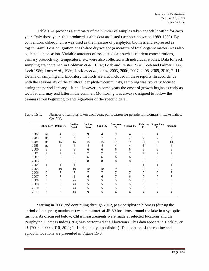
Nearshore Evaluation
October 15, 2013
Version 10.e
Page 134
Table 15-1 provides a summary of the number of samples taken at each location for each
year. Only those years that produced usable data are listed (see note above on 1989-1992). By
convention, chlorophyll a was used as the measure of periphyton biomass and expressed as
mg chl a/m2. Loss on ignition or ash-free dry weight (a measure of total organic matter) was also
collected on occasion. Variable amounts of associated data such as nutrient concentrations,
primary productivity, temperature, etc. were also collected with individual studies. Data for each
sampling are contained in Goldman et al., 1982; Loeb and Reuter 1984; Loeb and Palmer 1985;
Loeb 1986; Loeb et al., 1986; Hackley et al., 2004, 2005, 2006, 2007, 2008, 2009, 2010, 2011.
Details of sampling and laboratory methods are also included in these reports. In accordance
with the seasonality of the eulittoral periphyton community, sampling was typically focused
during the period January – June. However, in some years the onset of growth begins as early as
October and may end latter in the summer. Monitoring was always designed to follow the
biomass from beginning to end regardless of the specific date.
Table 15-1. Number of samples taken each year, per location for periphyton biomass in Lake Tahoe,
CA-NV.
Starting in 2008 and continuing through 2012, peak periphyton biomass (during the
period of the spring maximum) was monitored at 45-50 locations around the lake in a synoptic
fashion. As discussed below, Chl a measurements were made at selected locations and the
Periphyton Biomass Index (PBI) was performed at all locations. This data appears in Hackley et
al. (2008, 2009, 2010, 2011; 2012 data not yet published). The location of the routine and
synoptic locations are presented in Figure 15-3.
Tahoe City Dollar Pt.Incline
Condo
Incline
WestSand Pt.
Deadman
Pt.Zephyr Pt.
Rubicon
Pt.
Sugar Pine
Pt. Pineland
1982 ns 4 9 9 4 9 4 9 4 9
1983 ns 7 7 7 7 7 7 7 7 8
1984 ns 15 15 15 15 15 14 14 14 14
1985 ns 4 4 4 4 4 4 3 4 4
2000 6 6 6 6 6 6 6 6 6 6
2001 7 7 7 7 7 7 7 7 7 7
2002 6 8 6 6 6 6 6 6 5 6
2003 8 7 8 8 8 8 8 8 8 8
2004 1 1 1 1 1 1 1 1 1 1
2005 10 10 10 10 10 9 10 10 10 9
2006 7 7 7 7 7 7 7 7 7 7
2007 7 7 3 6 6 7 6 7 7 7
2008 5 5 ns 5 5 5 5 5 5 5
2009 5 5 ns 5 5 5 5 5 5 5
2010 5 5 ns 5 5 5 5 5 5 5
2011 6 5 ns 9 5 4 4 4 4 4
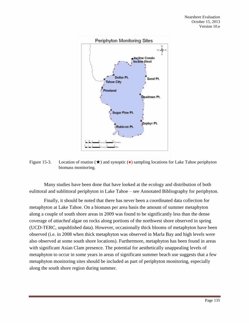
Nearshore Evaluation
October 15, 2013
Version 10.e
Page 135
Figure 15-3. Location of routine (★) and synoptic (●) sampling locations for Lake Tahoe periphyton
biomass monitoring.
Many studies have been done that have looked at the ecology and distribution of both
eulittoral and sublittoral periphyton in Lake Tahoe – see Annotated Bibliography for periphyton.
Finally, it should be noted that there has never been a coordinated data collection for
metaphyton at Lake Tahoe. On a biomass per area basis the amount of summer metaphyton
along a couple of south shore areas in 2009 was found to be significantly less than the dense
coverage of attached algae on rocks along portions of the northwest shore observed in spring
(UCD-TERC, unpublished data). However, occasionally thick blooms of metaphyton have been
observed (i.e. in 2008 when thick metaphyton was observed in Marla Bay and high levels were
also observed at some south shore locations). Furthermore, metaphyton has been found in areas
with significant Asian Clam presence. The potential for aesthetically unappealing levels of
metaphyton to occur in some years in areas of significant summer beach use suggests that a few
metaphyton monitoring sites should be included as part of periphyton monitoring, especially
along the south shore region during summer.
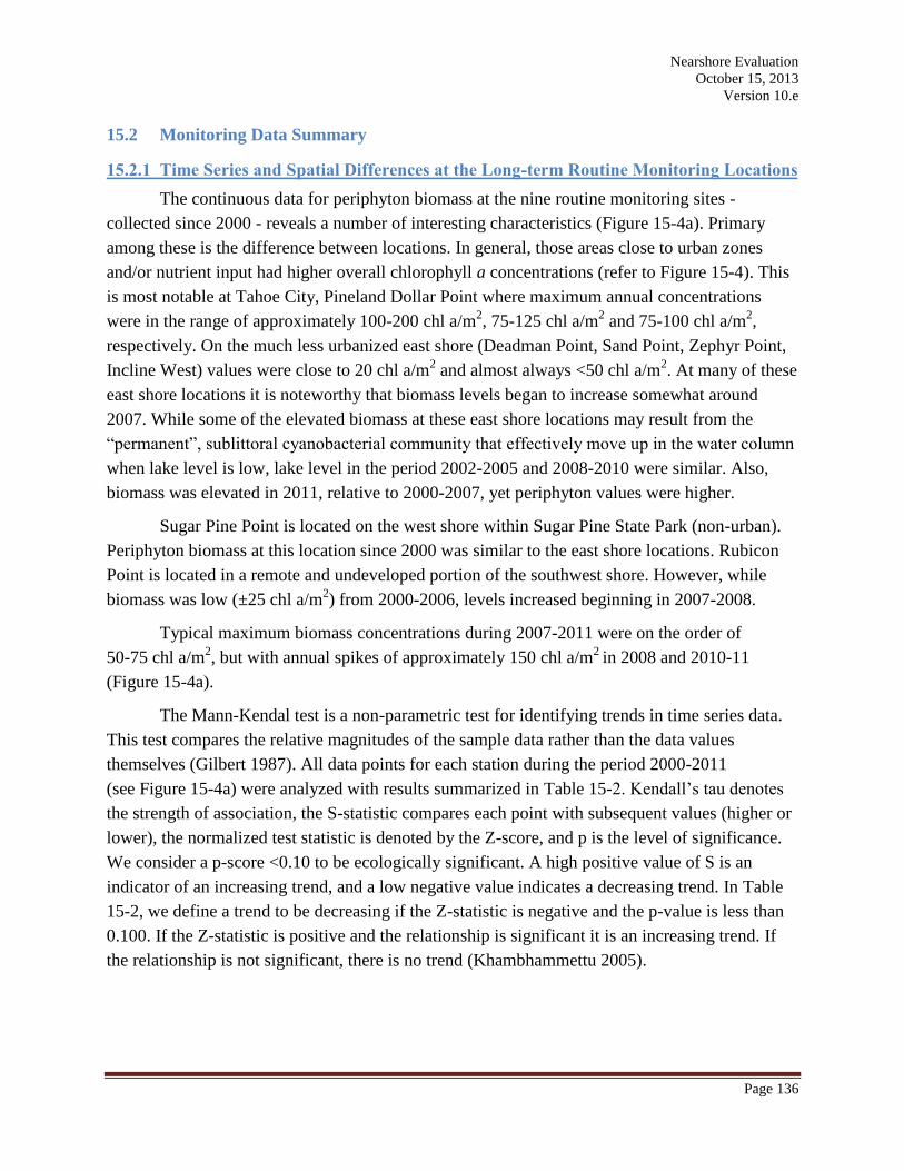
Nearshore Evaluation
October 15, 2013
Version 10.e
Page 136
15.2 Monitoring Data Summary
15.2.1 Time Series and Spatial Differences at the Long-term Routine Monitoring Locations
The continuous data for periphyton biomass at the nine routine monitoring sites -
collected since 2000 - reveals a number of interesting characteristics (Figure 15-4a). Primary
among these is the difference between locations. In general, those areas close to urban zones
and/or nutrient input had higher overall chlorophyll a concentrations (refer to Figure 15-4). This
is most notable at Tahoe City, Pineland Dollar Point where maximum annual concentrations
were in the range of approximately 100-200 chl a/m2, 75-125 chl a/m
2 and 75-100 chl a/m
2,
respectively. On the much less urbanized east shore (Deadman Point, Sand Point, Zephyr Point,
Incline West) values were close to 20 chl a/m2 and almost always <50 chl a/m
2. At many of these
east shore locations it is noteworthy that biomass levels began to increase somewhat around
2007. While some of the elevated biomass at these east shore locations may result from the
“permanent”, sublittoral cyanobacterial community that effectively move up in the water column
when lake level is low, lake level in the period 2002-2005 and 2008-2010 were similar. Also,
biomass was elevated in 2011, relative to 2000-2007, yet periphyton values were higher.
Sugar Pine Point is located on the west shore within Sugar Pine State Park (non-urban).
Periphyton biomass at this location since 2000 was similar to the east shore locations. Rubicon
Point is located in a remote and undeveloped portion of the southwest shore. However, while
biomass was low (±25 chl a/m2) from 2000-2006, levels increased beginning in 2007-2008.
Typical maximum biomass concentrations during 2007-2011 were on the order of
50-75 chl a/m2, but with annual spikes of approximately 150 chl a/m
2 in 2008 and 2010-11
(Figure 15-4a).
The Mann-Kendal test is a non-parametric test for identifying trends in time series data.
This test compares the relative magnitudes of the sample data rather than the data values
themselves (Gilbert 1987). All data points for each station during the period 2000-2011
(see Figure 15-4a) were analyzed with results summarized in Table 15-2. Kendall’s tau denotes
the strength of association, the S-statistic compares each point with subsequent values (higher or
lower), the normalized test statistic is denoted by the Z-score, and p is the level of significance.
We consider a p-score <0.10 to be ecologically significant. A high positive value of S is an
indicator of an increasing trend, and a low negative value indicates a decreasing trend. In Table
15-2, we define a trend to be decreasing if the Z-statistic is negative and the p-value is less than
0.100. If the Z-statistic is positive and the relationship is significant it is an increasing trend. If
the relationship is not significant, there is no trend (Khambhammettu 2005).
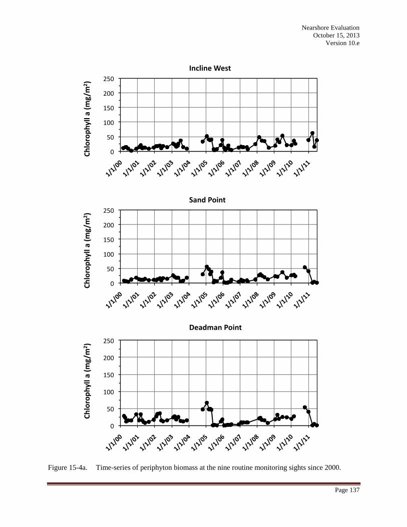
Nearshore Evaluation
October 15, 2013
Version 10.e
Page 137
Figure 15-4a. Time-series of periphyton biomass at the nine routine monitoring sights since 2000.
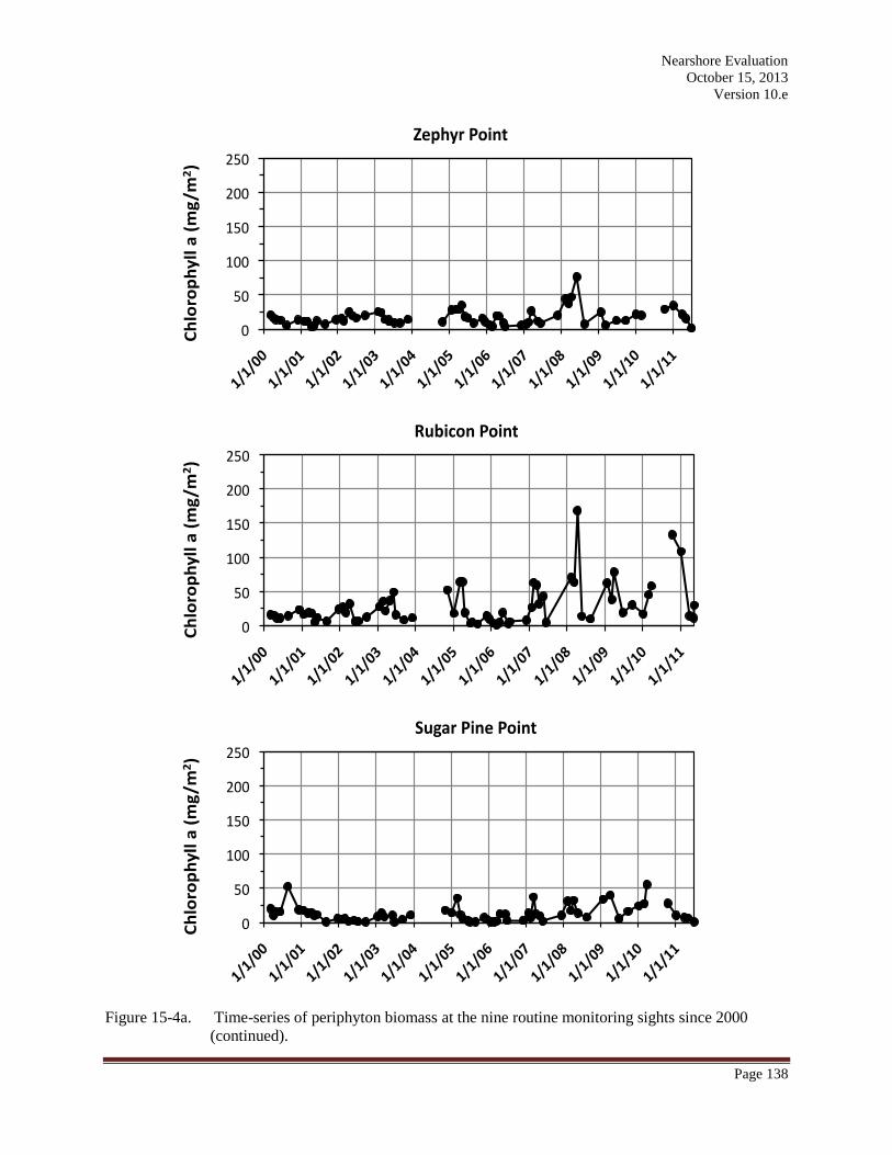
Nearshore Evaluation
October 15, 2013
Version 10.e
Page 138
Figure 15-4a. Time-series of periphyton biomass at the nine routine monitoring sights since 2000
(continued).
Nearshore Evaluation
October 15, 2013
Version 10.e
Page 139
Figure 15-4a. Time-series of periphyton biomass at the nine routine monitoring sights since 2000
(continued).
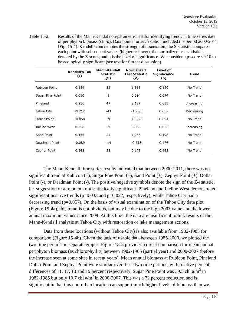
Nearshore Evaluation
October 15, 2013
Version 10.e
Page 140
Table 15-2. Results of the Mann-Kendal non-parametric test for identifying trends in time series data
of periphyton biomass (chl-a). Data points for each station included the period 2000-2011
(Fig. 15-4). Kendall’s tau denotes the strength of association, the S-statistic compares
each point with subsequent values (higher or lower), the normalized test statistic is
denoted by the Z-score, and p is the level of significance. We consider a p-score <0.10 to
be ecologically significant (see text for further discussion).
The Mann-Kendall time series results indicated that between 2000-2011, there was no
significant trend at Rubicon (+), Sugar Pine Point (+), Sand Point (+), Zephyr Point (+), Dollar
Point (-), or Deadman Point (-). The positive/negative symbols denote the sign of the Z-statistic,
i.e. suggestion of a trend but not statistically significant. Pineland and Incline West demonstrated
significant positive trends (p=0.033 and p=0.022, respectively), while Tahoe City had a
decreasing trend (p=0.057). On the basis of visual examination of the Tahoe City data plot
(Figure 15-4a), this trend is not obvious, but may be due to the high 2003 value and the lower
annual maximum values since 2009. At this time, the data are insufficient to link results of the
Mann-Kendall analysis at Tahoe City with restoration or lake management actions.
Data from these locations (without Tahoe City) is also available from 1982-1985 for
comparison (Figure 15-4b). Given the lack of usable data between 1985-2000, we plotted the
two time periods on separate graphs. Figure 15-5 provides a direct comparison for mean annual
periphyton biomass (as chlorophyll a) between 1982-1985 (partial year) and 2000-2007 (before
the increase seen at some sites in recent years). Mean annual biomass at Rubicon Point, Pineland,
Dollar Point and Zephyr Point were similar over these two time periods, with relative percent
differences of 11, 17, 13 and 19 percent respectively. Sugar Pine Point was 39.5 chl a/m2 in
1982-1985 but only 10.7 chl a/m2
in 2000-2007. This was a 72 percent reduction and is
significant in that this non-urban location can support much higher levels of biomass than we
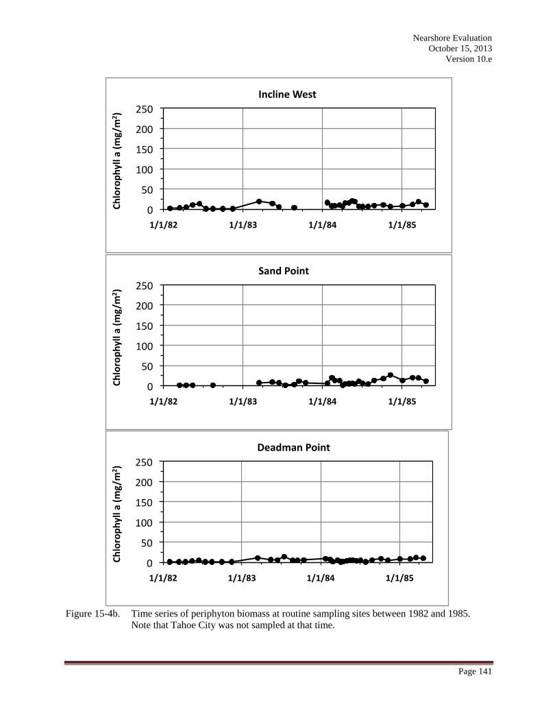
Nearshore Evaluation
October 15, 2013
Version 10.e
Page 141
Figure 15-4b. Time series of periphyton biomass at routine sampling sites between 1982 and 1985.
Note that Tahoe City was not sampled at that time.
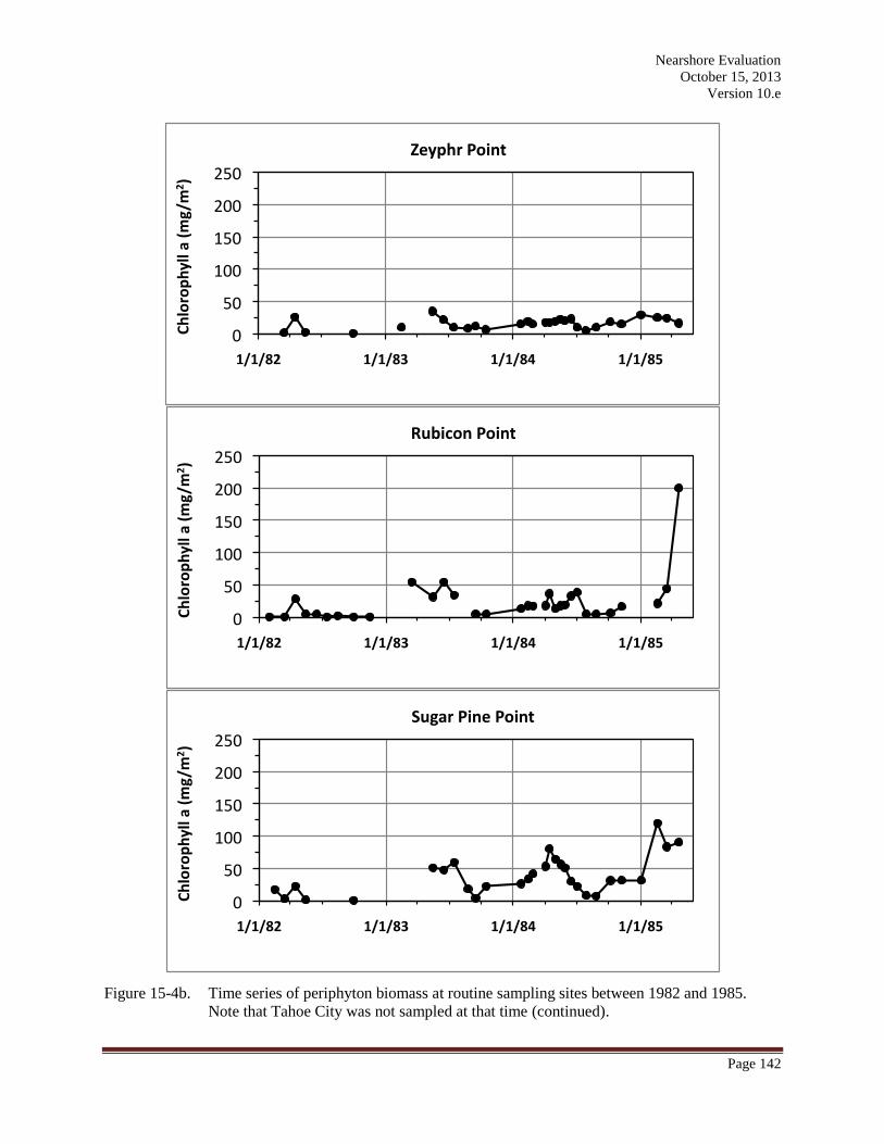
Nearshore Evaluation
October 15, 2013
Version 10.e
Page 142
Figure 15-4b. Time series of periphyton biomass at routine sampling sites between 1982 and 1985.
Note that Tahoe City was not sampled at that time (continued).
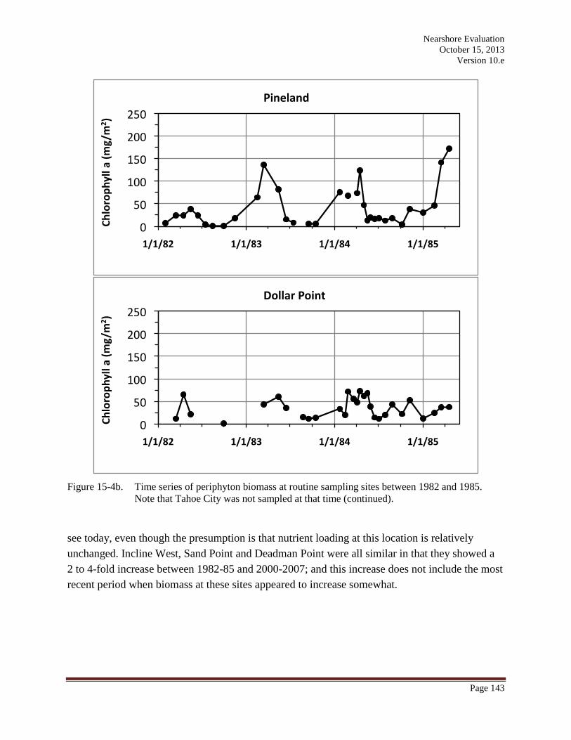
Nearshore Evaluation
October 15, 2013
Version 10.e
Page 143
Figure 15-4b. Time series of periphyton biomass at routine sampling sites between 1982 and 1985.
Note that Tahoe City was not sampled at that time (continued).
see today, even though the presumption is that nutrient loading at this location is relatively
unchanged. Incline West, Sand Point and Deadman Point were all similar in that they showed a
2 to 4-fold increase between 1982-85 and 2000-2007; and this increase does not include the most
recent period when biomass at these sites appeared to increase somewhat.
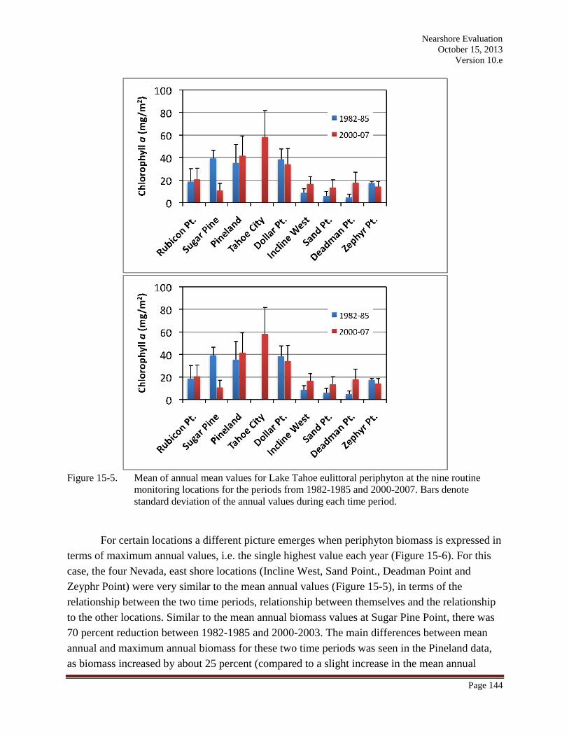
Nearshore Evaluation
October 15, 2013
Version 10.e
Page 144
Figure 15-5. Mean of annual mean values for Lake Tahoe eulittoral periphyton at the nine routine
monitoring locations for the periods from 1982-1985 and 2000-2007. Bars denote
standard deviation of the annual values during each time period.
For certain locations a different picture emerges when periphyton biomass is expressed in
terms of maximum annual values, i.e. the single highest value each year (Figure 15-6). For this
case, the four Nevada, east shore locations (Incline West, Sand Point., Deadman Point and
Zeyphr Point) were very similar to the mean annual values (Figure 15-5), in terms of the
relationship between the two time periods, relationship between themselves and the relationship
to the other locations. Similar to the mean annual biomass values at Sugar Pine Point, there was
70 percent reduction between 1982-1985 and 2000-2003. The main differences between mean
annual and maximum annual biomass for these two time periods was seen in the Pineland data,
as biomass increased by about 25 percent (compared to a slight increase in the mean annual
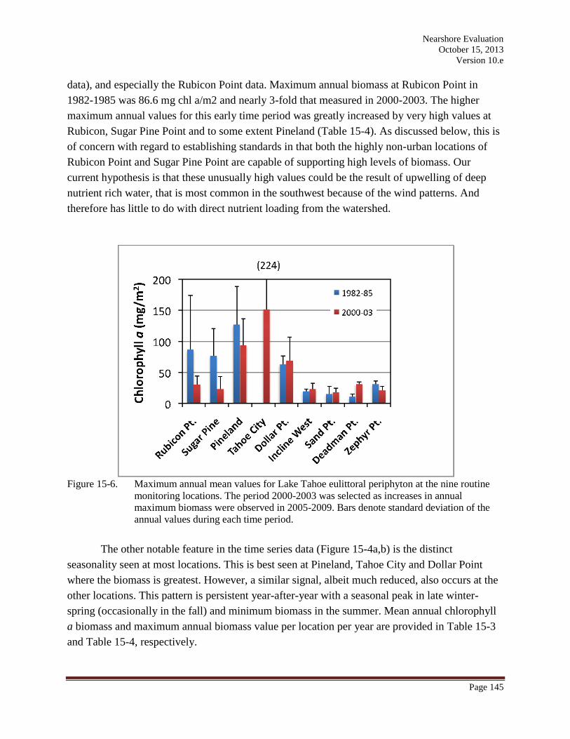
Nearshore Evaluation
October 15, 2013
Version 10.e
Page 145
data), and especially the Rubicon Point data. Maximum annual biomass at Rubicon Point in
1982-1985 was 86.6 mg chl a/m2 and nearly 3-fold that measured in 2000-2003. The higher
maximum annual values for this early time period was greatly increased by very high values at
Rubicon, Sugar Pine Point and to some extent Pineland (Table 15-4). As discussed below, this is
of concern with regard to establishing standards in that both the highly non-urban locations of
Rubicon Point and Sugar Pine Point are capable of supporting high levels of biomass. Our
current hypothesis is that these unusually high values could be the result of upwelling of deep
nutrient rich water, that is most common in the southwest because of the wind patterns. And
therefore has little to do with direct nutrient loading from the watershed.
Figure 15-6. Maximum annual mean values for Lake Tahoe eulittoral periphyton at the nine routine
monitoring locations. The period 2000-2003 was selected as increases in annual
maximum biomass were observed in 2005-2009. Bars denote standard deviation of the
annual values during each time period.
The other notable feature in the time series data (Figure 15-4a,b) is the distinct
seasonality seen at most locations. This is best seen at Pineland, Tahoe City and Dollar Point
where the biomass is greatest. However, a similar signal, albeit much reduced, also occurs at the
other locations. This pattern is persistent year-after-year with a seasonal peak in late winter-
spring (occasionally in the fall) and minimum biomass in the summer. Mean annual chlorophyll
a biomass and maximum annual biomass value per location per year are provided in Table 15-3
and Table 15-4, respectively.
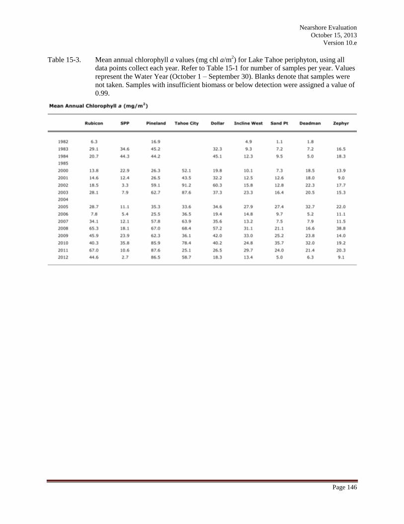
Nearshore Evaluation
October 15, 2013
Version 10.e
Page 146
Table 15-3. Mean annual chlorophyll a values (mg chl a/m2) for Lake Tahoe periphyton, using all
data points collect each year. Refer to Table 15-1 for number of samples per year. Values
represent the Water Year (October 1 – September 30). Blanks denote that samples were
not taken. Samples with insufficient biomass or below detection were assigned a value of
0.99.
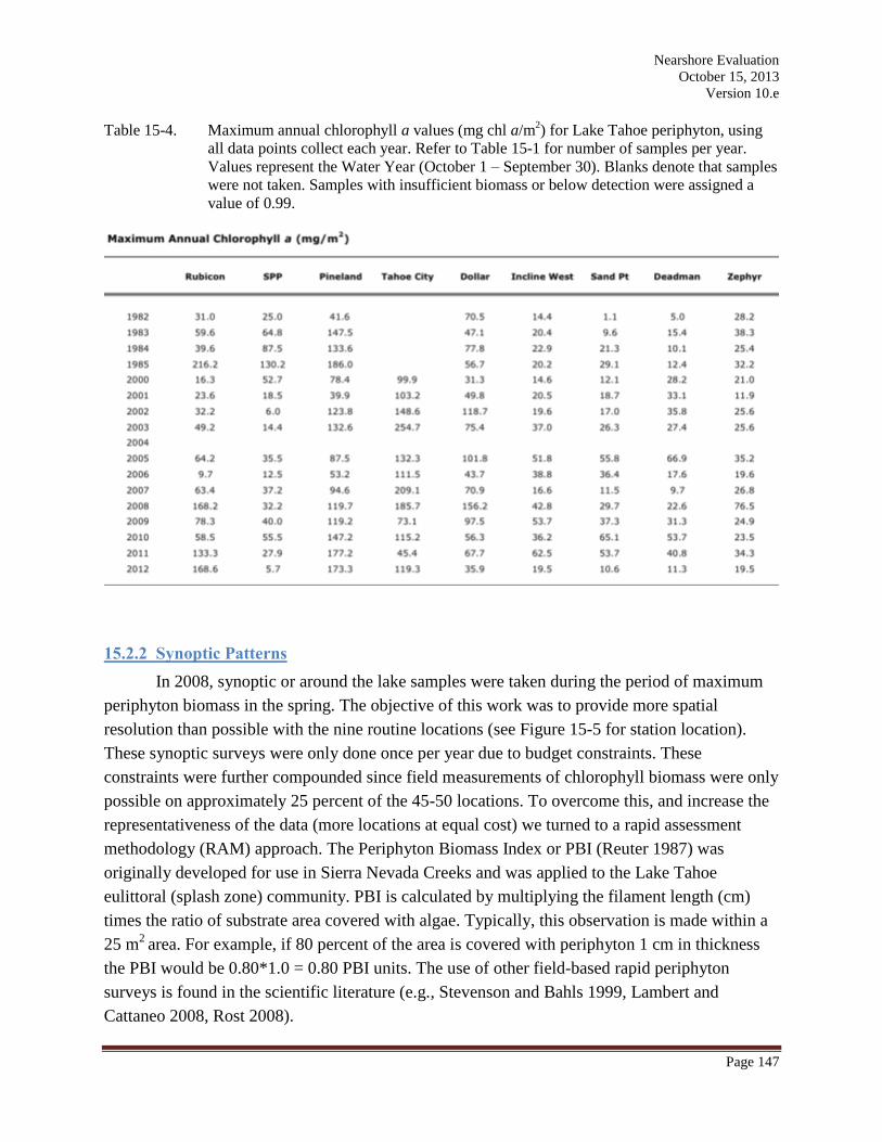
Nearshore Evaluation
October 15, 2013
Version 10.e
Page 147
Table 15-4. Maximum annual chlorophyll a values (mg chl a/m2) for Lake Tahoe periphyton, using
all data points collect each year. Refer to Table 15-1 for number of samples per year.
Values represent the Water Year (October 1 – September 30). Blanks denote that samples
were not taken. Samples with insufficient biomass or below detection were assigned a
value of 0.99.
15.2.2 Synoptic Patterns
In 2008, synoptic or around the lake samples were taken during the period of maximum
periphyton biomass in the spring. The objective of this work was to provide more spatial
resolution than possible with the nine routine locations (see Figure 15-5 for station location).
These synoptic surveys were only done once per year due to budget constraints. These
constraints were further compounded since field measurements of chlorophyll biomass were only
possible on approximately 25 percent of the 45-50 locations. To overcome this, and increase the
representativeness of the data (more locations at equal cost) we turned to a rapid assessment
methodology (RAM) approach. The Periphyton Biomass Index or PBI (Reuter 1987) was
originally developed for use in Sierra Nevada Creeks and was applied to the Lake Tahoe
eulittoral (splash zone) community. PBI is calculated by multiplying the filament length (cm)
times the ratio of substrate area covered with algae. Typically, this observation is made within a
25 m2
area. For example, if 80 percent of the area is covered with periphyton 1 cm in thickness
the PBI would be 0.80*1.0 = 0.80 PBI units. The use of other field-based rapid periphyton
surveys is found in the scientific literature (e.g., Stevenson and Bahls 1999, Lambert and
Cattaneo 2008, Rost 2008).
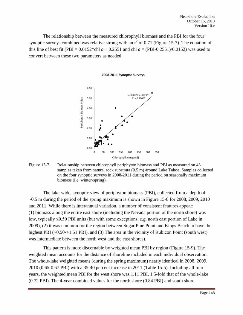
Nearshore Evaluation
October 15, 2013
Version 10.e
Page 148
The relationship between the measured chlorophyll biomass and the PBI for the four
synoptic surveys combined was relative strong with an r2 of 0.71 (Figure 15-7). The equation of
this line of best fit (PBI = 0.0152*chl a + 0.2551 and chl a = (PBI-0.2551)/0.0152) was used to
convert between these two parameters as needed.
Figure 15-7. Relationship between chlorophyll periphyton biomass and PBI as measured on 43
samples taken from natural rock substrata (0.5 m) around Lake Tahoe. Samples collected
on the four synoptic surveys in 2008-2011 during the period on seasonally maximum
biomass (i.e. winter-spring).
The lake-wide, synoptic view of periphyton biomass (PBI), collected from a depth of
~0.5 m during the period of the spring maximum is shown in Figure 15-8 for 2008, 2009, 2010
and 2011. While there is interannual variation, a number of consistent features appear:
(1) biomass along the entire east shore (including the Nevada portion of the north shore) was
low, typically ≤0.50 PBI units (but with some exceptions, e.g. north east portion of Lake in
2009), (2) it was common for the region between Sugar Pine Point and Kings Beach to have the
highest PBI (~0.50->1.51 PBI), and (3) The area in the vicinity of Rubicon Point (south west)
was intermediate between the north west and the east shores).
This pattern is more discernable by weighted mean PBI by region (Figure 15-9). The
weighted mean accounts for the distance of shoreline included in each individual observation.
The whole-lake weighted means (during the spring maximum) nearly identical in 2008, 2009,
2010 (0.65-0.67 PBI) with a 35-40 percent increase in 2011 (Table 15-5). Including all four
years, the weighted mean PBI for the west shore was 1.11 PBI, 1.5-fold that of the whole-lake
(0.72 PBI). The 4-year combined values for the north shore (0.84 PBI) and south shore
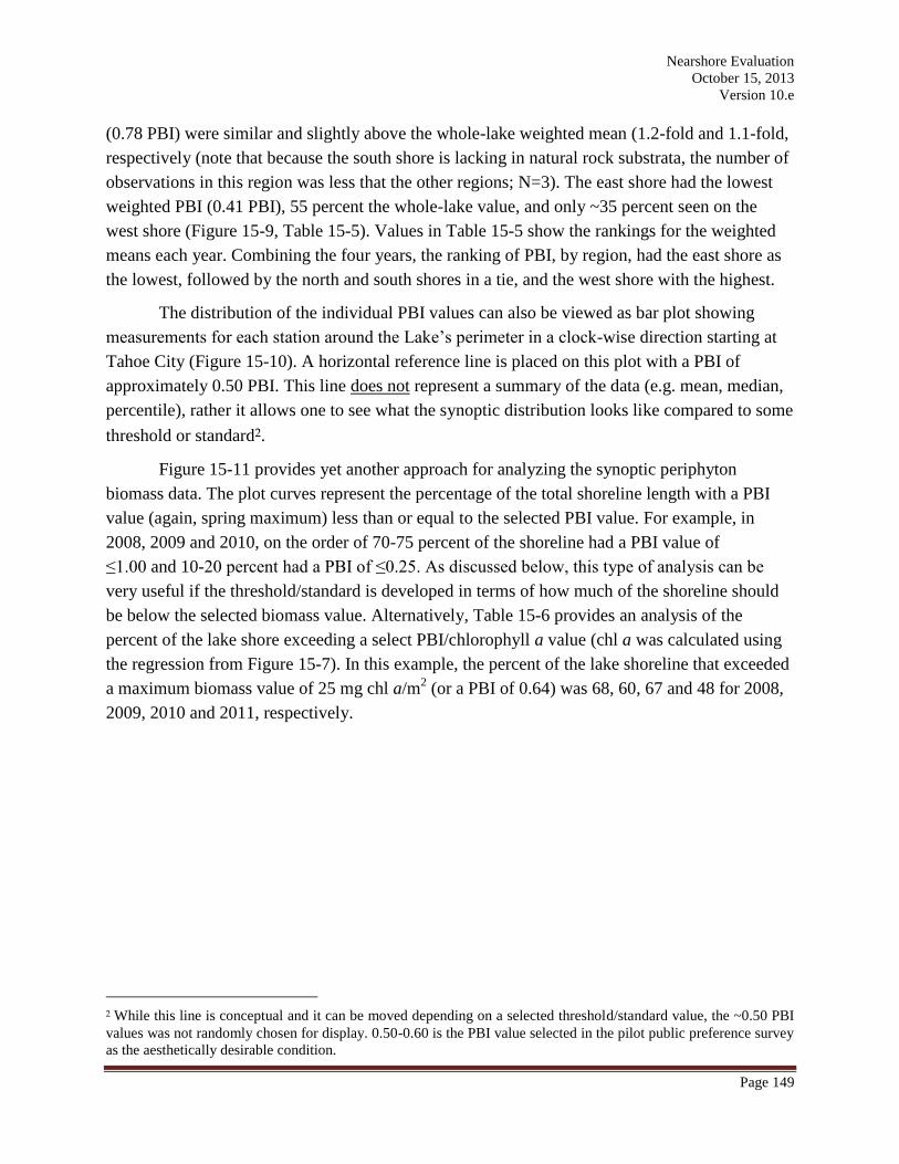
Nearshore Evaluation
October 15, 2013
Version 10.e
Page 149
(0.78 PBI) were similar and slightly above the whole-lake weighted mean (1.2-fold and 1.1-fold,
respectively (note that because the south shore is lacking in natural rock substrata, the number of
observations in this region was less that the other regions; N=3). The east shore had the lowest
weighted PBI (0.41 PBI), 55 percent the whole-lake value, and only ~35 percent seen on the
west shore (Figure 15-9, Table 15-5). Values in Table 15-5 show the rankings for the weighted
means each year. Combining the four years, the ranking of PBI, by region, had the east shore as
the lowest, followed by the north and south shores in a tie, and the west shore with the highest.
The distribution of the individual PBI values can also be viewed as bar plot showing
measurements for each station around the Lake’s perimeter in a clock-wise direction starting at
Tahoe City (Figure 15-10). A horizontal reference line is placed on this plot with a PBI of
approximately 0.50 PBI. This line does not represent a summary of the data (e.g. mean, median,
percentile), rather it allows one to see what the synoptic distribution looks like compared to some
threshold or standard2.
Figure 15-11 provides yet another approach for analyzing the synoptic periphyton
biomass data. The plot curves represent the percentage of the total shoreline length with a PBI
value (again, spring maximum) less than or equal to the selected PBI value. For example, in
2008, 2009 and 2010, on the order of 70-75 percent of the shoreline had a PBI value of
≤1.00 and 10-20 percent had a PBI of ≤0.25. As discussed below, this type of analysis can be
very useful if the threshold/standard is developed in terms of how much of the shoreline should
be below the selected biomass value. Alternatively, Table 15-6 provides an analysis of the
percent of the lake shore exceeding a select PBI/chlorophyll a value (chl a was calculated using
the regression from Figure 15-7). In this example, the percent of the lake shoreline that exceeded
a maximum biomass value of 25 mg chl a/m2 (or a PBI of 0.64) was 68, 60, 67 and 48 for 2008,
2009, 2010 and 2011, respectively.
2 While this line is conceptual and it can be moved depending on a selected threshold/standard value, the ~0.50 PBI
values was not randomly chosen for display. 0.50-0.60 is the PBI value selected in the pilot public preference survey
as the aesthetically desirable condition.
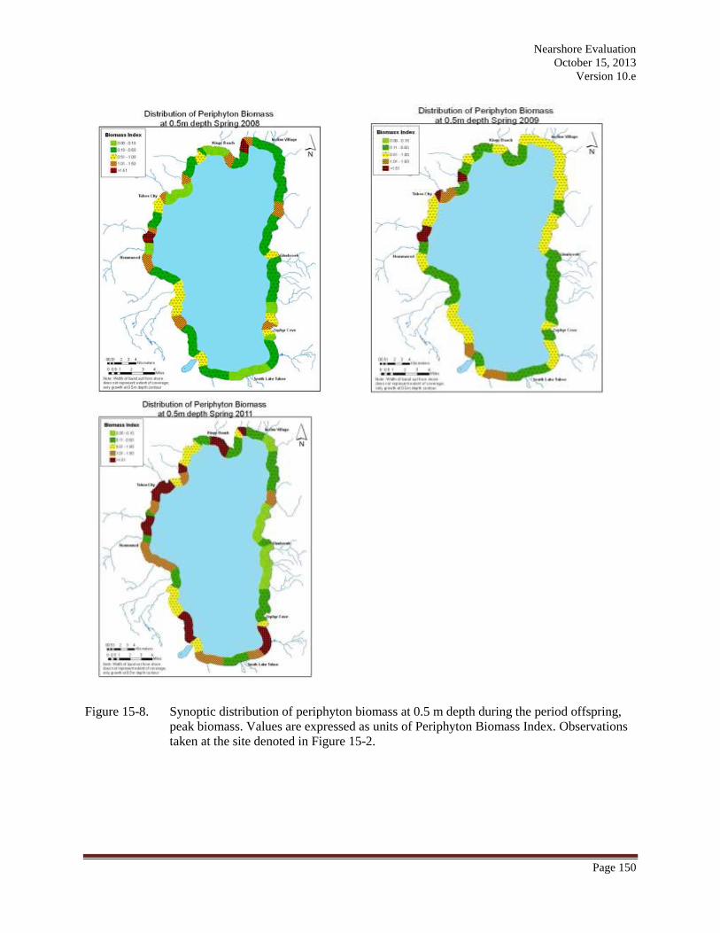
Nearshore Evaluation
October 15, 2013
Version 10.e
Page 150
Figure 15-8. Synoptic distribution of periphyton biomass at 0.5 m depth during the period offspring,
peak biomass. Values are expressed as units of Periphyton Biomass Index. Observations
taken at the site denoted in Figure 15-2.
Nearshore Evaluation
October 15, 2013
Version 10.e
Page 151
Figure 15-9. PBI distribution by geographic region during the period of spring, maximum biomass.
Values are weighted based on the actual shore length covered by each observation point.
Table 15-5. Regional spring, maximum PBI data as plotted in Figure 15-9. Includes other terms to
define periphyton distribution.
LAKE-WIDE NORTH SHORE EAST SHORE SOUTH SHORE WEST SHORE
2008 2009 2010 2011 2008 2009 2010 2011 2008 2009 2010 2011 2008 2009 2010 2011 2008 2009 2010 2011
Mean (weighted) 0.65 0.67 0.65 0.91 0.73 0.81 0.60 1.22 0.43 0.51 0.25 0.44 0.38 0.87 0.83 1.04 0.99 0.76 1.35 1.35
Mean 0.78 0.75 0.86 1.06 0.86 0.85 0.71 1.18 0.49 0.48 0.28 0.47 0.46 0.73 0.75 1.10 1.1 0.91 1.44 1.52
SD 0.80 0.80 1.07 1.01 0.86 1.02 0.76 0.83 0.39 0.24 0.14 0.52 0.44 0.60 0.30 0.39 1.03 0.88 1.54 1.40
SE 0.12 0.12 0.17 0.14 0.21 0.25 0.18 0.19 0.11 0.07 0.10 0.13 0.25 0.35 0.17 0.23 0.32 0.25 0.36 0.36
n 43 45 41 0.14 16 17 17 19 13 13 8 16 3 3 3 3 11 12 16 15
CI 95% 0.24 0.23 0.33 0.14 0.42 0.48 0.36 0.37 0.21 0.13 0.10 0.25 0.50 0.68 0.34 0.44 0.61 0.49 0.75 0.71
25th percentile 0.21 0.35 0.21 0.14 0.24 0.35 0.21 0.52 0.2 0.30 0.26 0.09 0.21 0.43 0.59 0.44 0.34 0.39 0.30 0.65
50th percentile (median) 0.48 0.49 0.42 0.14 0.43 0.45 0.42 0.90 0.32 0.40 0.29 0.35 0.30 0.70 0.70 0.90 0.88 0.58 0.83 1.20
75th percentile 1.07 0.75 0.86 0.14 1.36 0.85 0.64 1.71 0.90 0.63 0.33 0.58 0.63 1.03 0.89 1.08 1.52 1.02 2.88 1.89
Min 0.00 0.14 0.01 0.14 0.02 0.14 0.12 0.16 0.08 0.20 0.01 0.00 0.12 0.15 0.48 0.72 0.00 0.21 0.08 0.12
Max 3.00 4.00 4.95 0.14 2.56 4.00 2.70 2.70 1.08 1.00 0.48 1.60 0.96 1.35 1.08 1.50 3.00 3.15 4.95 5.50
2008 2009 2010 2011
North East South West North East South West North East South West North East South West
Mean (weighted) 0.73 0.43 0.38 0.99 0.81 0.51 0.87 0.76 0.60 0.25 0.83 1.35 1.22 0.44 1.04 1.35
Mean 0.86 0.49 0.46 1.1 0.85 0.48 0.73 0.91 0.71 0.28 0.75 1.44 1.18 0.47 1.10 1.52
SD 0.86 0.39 0.44 1.03 1.02 0.24 0.60 0.88 0.76 0.14 0.30 1.54 0.83 0.52 0.39 1.40
SE 0.21 0.11 0.25 0.32 0.25 0.07 0.35 0.25 0.18 0.10 0.17 0.36 0.19 0.13 0.23 0.36
n 16 13 3 11 17 13 3 12 17 8 3 16 19 16 3 15
CI 95% 0.42 0.21 0.5 0.61 0.48 0.13 0.68 0.49 0.36 0.10 0.34 0.75 0.37 0.25 0.44 0.71
25th percentile 0.24 0.2 0.21 0.34 0.35 0.30 0.43 0.39 0.21 0.26 0.59 0.30 0.52 0.09 0.44 0.65
50th percentile (median) 0.43 0.32 0.3 0.88 0.45 0.40 0.70 0.58 0.42 0.29 0.70 0.83 0.90 0.35 0.90 1.20
75th percentile 1.36 0.90 0.63 1.52 0.85 0.63 1.03 1.02 0.64 0.33 0.89 2.88 1.71 0.58 1.08 1.89
Min 0.02 0.08 0.12 0.00 0.14 0.20 0.15 0.21 0.12 0.01 0.48 0.08 0.16 0.00 0.72 0.12
Max 2.56 1.08 0.96 3.00 4.00 1.00 1.35 3.15 2.70 0.48 1.08 4.95 2.70 1.60 1.50 5.50
Weighted Mean Ranking 3 1 2 4 3 1 4 2 2 1 3 4 3 1 2 4
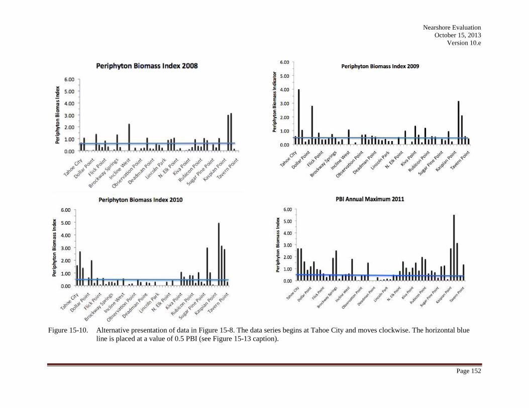
Nearshore Evaluation
October 15, 2013
Version 10.e
Page 152
Figure 15-10. Alternative presentation of data in Figure 15-8. The data series begins at Tahoe City and moves clockwise. The horizontal blue
line is placed at a value of 0.5 PBI (see Figure 15-13 caption).
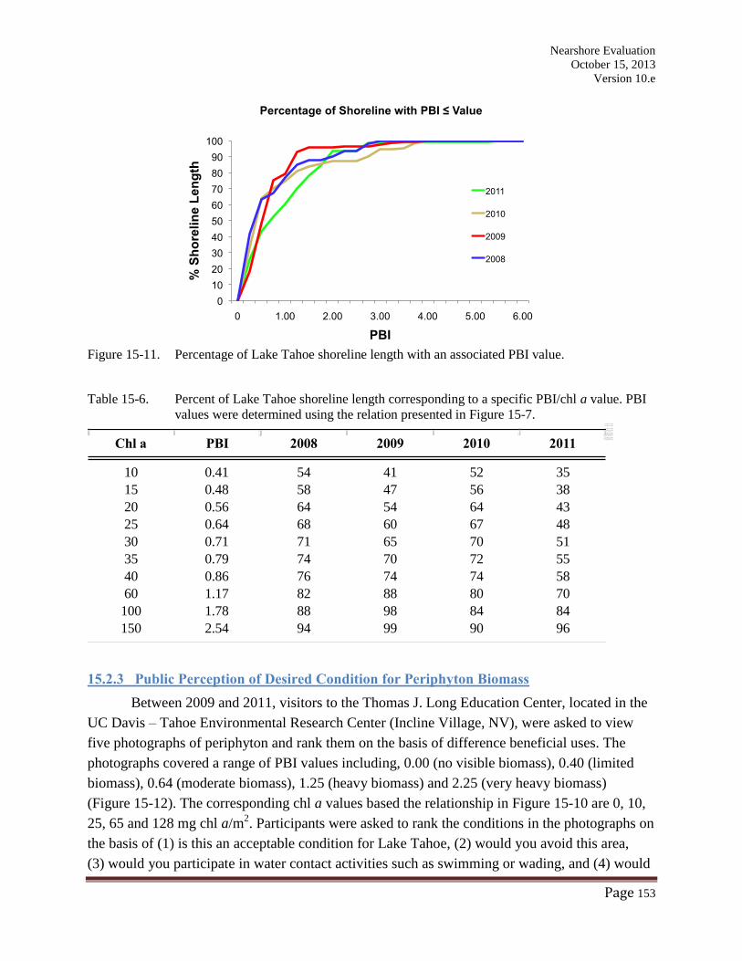
Nearshore Evaluation
October 15, 2013
Version 10.e
Page 153
Figure 15-11. Percentage of Lake Tahoe shoreline length with an associated PBI value.
Table 15-6. Percent of Lake Tahoe shoreline length corresponding to a specific PBI/chl a value. PBI
values were determined using the relation presented in Figure 15-7.
15.2.3 Public Perception of Desired Condition for Periphyton Biomass
Between 2009 and 2011, visitors to the Thomas J. Long Education Center, located in the
UC Davis – Tahoe Environmental Research Center (Incline Village, NV), were asked to view
five photographs of periphyton and rank them on the basis of difference beneficial uses. The
photographs covered a range of PBI values including, 0.00 (no visible biomass), 0.40 (limited
biomass), 0.64 (moderate biomass), 1.25 (heavy biomass) and 2.25 (very heavy biomass)
(Figure 15-12). The corresponding chl a values based the relationship in Figure 15-10 are 0, 10,
25, 65 and 128 mg chl a/m2. Participants were asked to rank the conditions in the photographs on
the basis of (1) is this an acceptable condition for Lake Tahoe, (2) would you avoid this area,
(3) would you participate in water contact activities such as swimming or wading, and (4) would
Chl a PBI 2008 2009 2010 2011
10 0.41 54 41 52 35
15 0.48 58 47 56 38
20 0.56 64 54 64 43
25 0.64 68 60 67 48
30 0.71 71 65 70 51
35 0.79 74 70 72 55
40 0.86 76 74 74 58
60 1.17 82 88 80 70
100 1.78 88 98 84 84
150 2.54 94 99 90 96
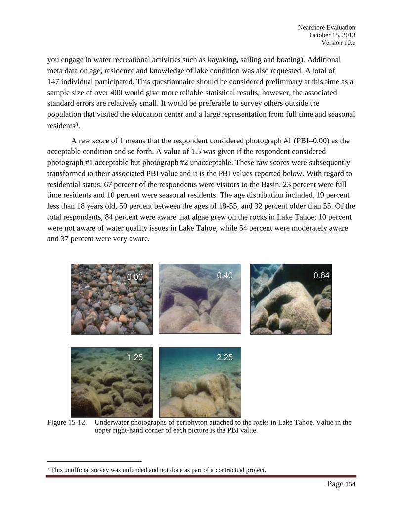
Nearshore Evaluation
October 15, 2013
Version 10.e
Page 154
you engage in water recreational activities such as kayaking, sailing and boating). Additional
meta data on age, residence and knowledge of lake condition was also requested. A total of
147 individual participated. This questionnaire should be considered preliminary at this time as a
sample size of over 400 would give more reliable statistical results; however, the associated
standard errors are relatively small. It would be preferable to survey others outside the
population that visited the education center and a large representation from full time and seasonal
residents3.
A raw score of 1 means that the respondent considered photograph #1 (PBI=0.00) as the
acceptable condition and so forth. A value of 1.5 was given if the respondent considered
photograph #1 acceptable but photograph #2 unacceptable. These raw scores were subsequently
transformed to their associated PBI value and it is the PBI values reported below. With regard to
residential status, 67 percent of the respondents were visitors to the Basin, 23 percent were full
time residents and 10 percent were seasonal residents. The age distribution included, 19 percent
less than 18 years old, 50 percent between the ages of 18-55, and 32 percent older than 55. Of the
total respondents, 84 percent were aware that algae grew on the rocks in Lake Tahoe; 10 percent
were not aware of water quality issues in Lake Tahoe, while 54 percent were moderately aware
and 37 percent were very aware.
Figure 15-12. Underwater photographs of periphyton attached to the rocks in Lake Tahoe. Value in the
upper right-hand corner of each picture is the PBI value.
3 This unofficial survey was unfunded and not done as part of a contractual project.
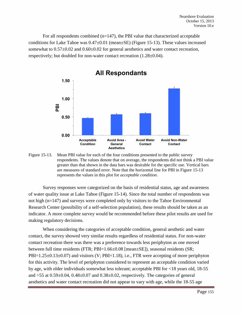
Nearshore Evaluation
October 15, 2013
Version 10.e
Page 155
For all respondents combined (n=147), the PBI value that characterized acceptable
conditions for Lake Tahoe was 0.47±0.01 (mean±SE) (Figure 15-13). These values increased
somewhat to 0.57±0.02 and 0.60±0.02 for general aesthetics and water contact recreation,
respectively; but doubled for non-water contact recreation (1.28±0.04).
Figure 15-13. Mean PBI value for each of the four conditions presented to the public survey
respondents. The values denote that on average, the respondents did not think a PBI value
greater than that shown in the data bars was desirable for the specific use. Vertical bars
are measures of standard error. Note that the horizontal line for PBI in Figure 15-13
represents the values in this plot for acceptable condition.
Survey responses were categorized on the basis of residential status, age and awareness
of water quality issue at Lake Tahoe (Figure 15-14). Since the total number of respondents was
not high (n=147) and surveys were completed only by visitors to the Tahoe Environmental
Research Center (possibility of a self-selection population), these results should be taken as an
indicator. A more complete survey would be recommended before these pilot results are used for
making regulatory decisions.
When considering the categories of acceptable condition, general aesthetic and water
contact, the survey showed very similar results regardless of residential status. For non-water
contact recreation there was there was a preference towards less periphyton as one moved
between full time residents (FTR; PBI=1.66±0.08 [mean±SE]), seasonal residents (SR;
PBI=1.25±0.13±0.07) and visitors (V; PBI=1.18), i.e., FTR were accepting of more periphyton
for this activity. The level of periphyton considered to represent an acceptable condition varied
by age, with older individuals somewhat less tolerant; acceptable PBI for <18 years old, 18-55
and >55 at 0.59±0.04, 0.48±0.07 and 0.38±0.02, respectively. The categories of general
aesthetics and water contact recreation did not appear to vary with age, while the 18-55 age
0.00
0.50
1.00
1.50
Acceptable
Condition
Avoid Area -
General
Aesthetics
Avoid Water
Contact
Avoid Non-Water
Contact
PB
I
All Respondants
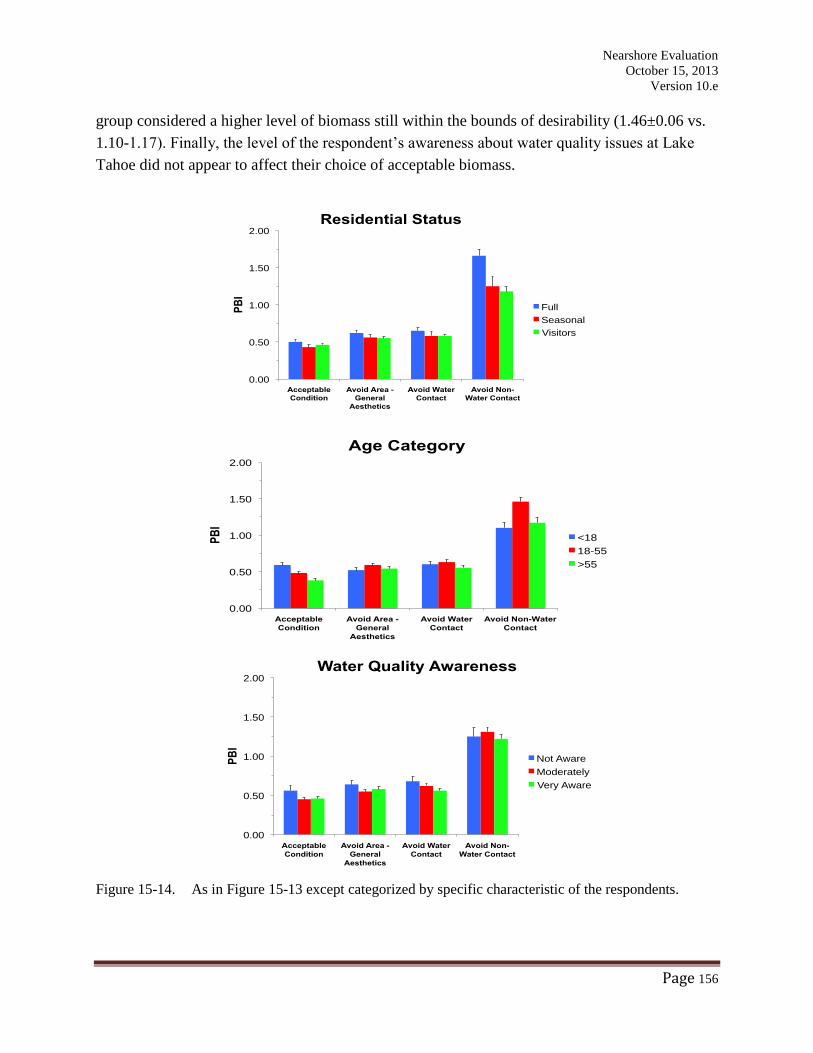
Nearshore Evaluation
October 15, 2013
Version 10.e
Page 156
group considered a higher level of biomass still within the bounds of desirability (1.46±0.06 vs.
1.10-1.17). Finally, the level of the respondent’s awareness about water quality issues at Lake
Tahoe did not appear to affect their choice of acceptable biomass.
Figure 15-14. As in Figure 15-13 except categorized by specific characteristic of the respondents.
0.00
0.50
1.00
1.50
2.00
Acceptable
Condition
Avoid Area -
General
Aesthetics
Avoid Water
Contact
Avoid Non-
Water Contact
PB
I
Residential Status
Full
Seasonal
Visitors
0.00
0.50
1.00
1.50
2.00
Acceptable
Condition
Avoid Area -
General
Aesthetics
Avoid Water
Contact
Avoid Non-Water
Contact
PB
I
Age Category
<18
18-55
>55
0.00
0.50
1.00
1.50
2.00
Acceptable
Condition
Avoid Area -
General
Aesthetics
Avoid Water
Contact
Avoid Non-
Water Contact
PB
I
Water Quality Awareness
Not Aware
Moderately
Very Aware
Nearshore Evaluation
October 15, 2013
Version 10.e
Page 157
15.3 Discussion of Reference Conditions
Identification of reference conditions is needed to begin the process of establishing
thresholds. A threshold represents a desired condition, but not necessarily a pristine condition or
a condition unaffected by anthropogenic inputs. Numerous factors go into the determination of a
desired condition (e.g. public preference, health and safety, protection of special ecosystem, cost
of implementation, the practical/logistical feasibility of ever achieving these conditions). All
these require consideration by the regulatory agencies, with public input, during an adoption
process. In this report we provide the scientific data and analysis that will help support this
process.
Based on the available data, and with the exception of using public opinion alone to
establish reference conditions (see Section B.3), the data from Lake Tahoe allow us to consider
reference condition in terms of both mean annual chlorophyll a and maximum annual
chlorophyll a. As previously discussed, we have used the relationship between chl a and PBI
(Figure 15-7) when data for one or the other is not available.
Mean annual chlorophyll a values are presented in Figure 15-4 and Figure 15-15. Since
there has been a statistically significant increase in biomass over time at certain locations
(see Table 15-2), we examined various time periods so determine the appropriateness of a
reference station designation. Using the 20 mg chl a/m2 value as the transition between
oligotrophic and mesotrophic as suggested by Dodds et al. (1998), mean annual biomass at
Incline West, Sand Point, Deadman Point and Zephyr Point was always less. This supports visual
observation by limnologists and research divers that these can be considered reference
conditions, at least for the northeast, east and southeast shorelines. Similarly, annual average
periphyton biomass at Pineland, Tahoe City and Dollar Point were also in excess of the 20 mg
chl a/m2
value and could not be considered reference stations. Interpretation of the Rubicon Point
and Sugar Pine Point stations on the west shore was more ambiguous in that exceedence of the
20 mg chl a/m2 value was dependent on the time period. During the period 1983-1985 when
sampling was initially started values of ~40 mg chl a/m2 were observed as compared to values
<20 mg chl a/m2 seen since 2000. Mean annual biomass at Rubicon Point in recent years (2007-
2009) has been high (34.1-45.9 mg chl a/m2) relative to earlier periods; therefore, these latter
values should not serve as a reference condition. Based on this analysis, our preliminary finding
is that the mean annual biomass levels at Rubicon Point, Sugar Pine, Point Incline West, Sand
Point, Deadman Point and Zephyr Point during the period 2000-2003 are indicative of reference
conditions – a mean of 15 mg/m2 with a range of 12-20 mg/m
2.
The distribution of maximumal annual periphyton was similar to that of mean annual
biomass (Figure 15-16 and Table 15-8). While mean annual biomass never exceeded the
nuisance value of 100 mg chl a/m2, as defined in the literature (see Section 2), the 150-200 mg
chl a/m2 threshold maximum annual biomass was exceeded 15 percent of the time at Rubicon
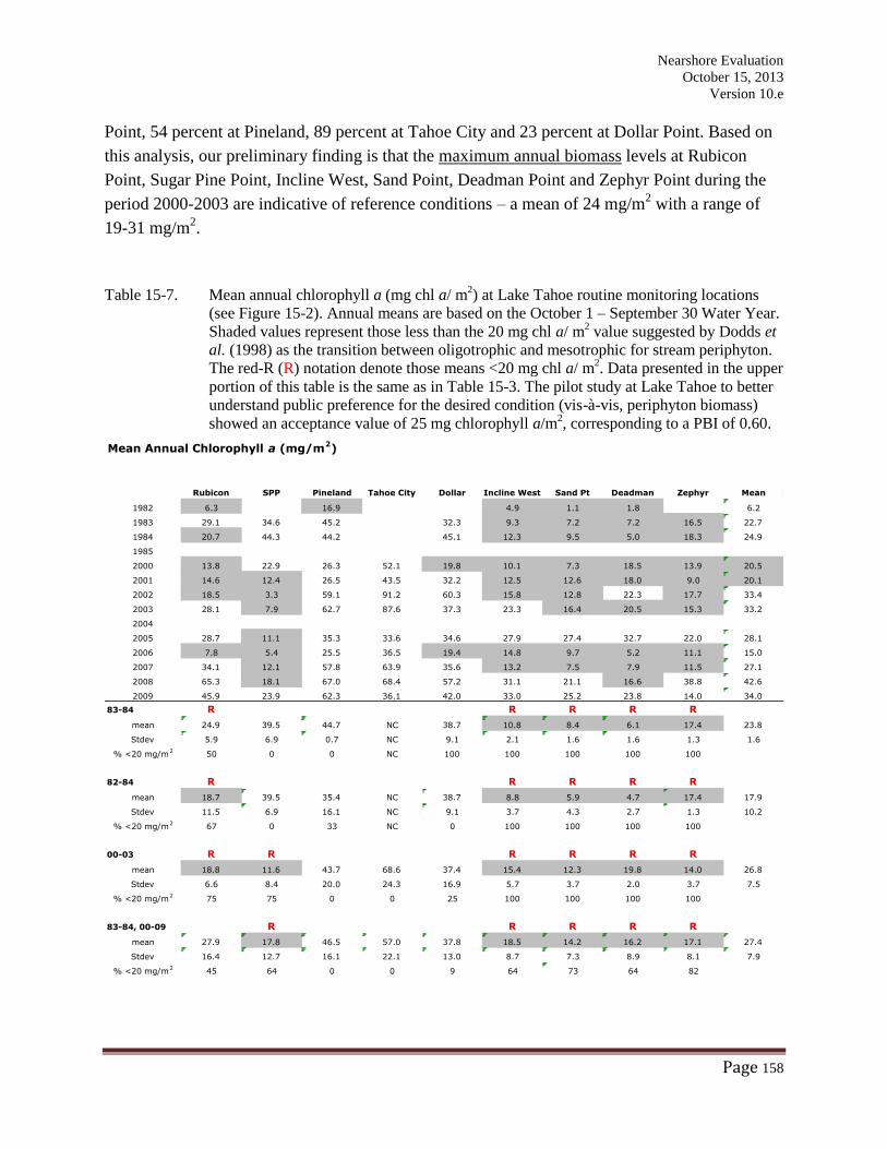
Nearshore Evaluation
October 15, 2013
Version 10.e
Page 158
Point, 54 percent at Pineland, 89 percent at Tahoe City and 23 percent at Dollar Point. Based on
this analysis, our preliminary finding is that the maximum annual biomass levels at Rubicon
Point, Sugar Pine Point, Incline West, Sand Point, Deadman Point and Zephyr Point during the
period 2000-2003 are indicative of reference conditions – a mean of 24 mg/m2 with a range of
19-31 mg/m2.
Table 15-7. Mean annual chlorophyll a (mg chl a/ m2) at Lake Tahoe routine monitoring locations
(see Figure 15-2). Annual means are based on the October 1 – September 30 Water Year.
Shaded values represent those less than the 20 mg chl a/ m2 value suggested by Dodds et
al. (1998) as the transition between oligotrophic and mesotrophic for stream periphyton.
The red-R (R) notation denote those means <20 mg chl a/ m2. Data presented in the upper
portion of this table is the same as in Table 15-3. The pilot study at Lake Tahoe to better
understand public preference for the desired condition (vis-à-vis, periphyton biomass)
showed an acceptance value of 25 mg chlorophyll a/m2, corresponding to a PBI of 0.60.
Mean Annual Chlorophyll a (mg/m2)
Rubicon SPP Pineland Tahoe City Dollar Incline West Sand Pt Deadman Zephyr Mean
1982 6.3 16.9 4.9 1.1 1.8 6.2
1983 29.1 34.6 45.2 32.3 9.3 7.2 7.2 16.5 22.7
1984 20.7 44.3 44.2 45.1 12.3 9.5 5.0 18.3 24.9
1985
2000 13.8 22.9 26.3 52.1 19.8 10.1 7.3 18.5 13.9 20.5
2001 14.6 12.4 26.5 43.5 32.2 12.5 12.6 18.0 9.0 20.1
2002 18.5 3.3 59.1 91.2 60.3 15.8 12.8 22.3 17.7 33.4
2003 28.1 7.9 62.7 87.6 37.3 23.3 16.4 20.5 15.3 33.2
2004
2005 28.7 11.1 35.3 33.6 34.6 27.9 27.4 32.7 22.0 28.1
2006 7.8 5.4 25.5 36.5 19.4 14.8 9.7 5.2 11.1 15.0
2007 34.1 12.1 57.8 63.9 35.6 13.2 7.5 7.9 11.5 27.1
2008 65.3 18.1 67.0 68.4 57.2 31.1 21.1 16.6 38.8 42.6
2009 45.9 23.9 62.3 36.1 42.0 33.0 25.2 23.8 14.0 34.0
83-84 R R R R R
mean 24.9 39.5 44.7 NC 38.7 10.8 8.4 6.1 17.4 23.8
Stdev 5.9 6.9 0.7 NC 9.1 2.1 1.6 1.6 1.3 1.6
% <20 mg/m2
50 0 0 NC 100 100 100 100 100
82-84 R R R R R
mean 18.7 39.5 35.4 NC 38.7 8.8 5.9 4.7 17.4 17.9
Stdev 11.5 6.9 16.1 NC 9.1 3.7 4.3 2.7 1.3 10.2
% <20 mg/m2
67 0 33 NC 0 100 100 100 100
00-03 R R R R R R
mean 18.8 11.6 43.7 68.6 37.4 15.4 12.3 19.8 14.0 26.8
Stdev 6.6 8.4 20.0 24.3 16.9 5.7 3.7 2.0 3.7 7.5
% <20 mg/m2
75 75 0 0 25 100 100 100 100
83-84, 00-09 R R R R R
mean 27.9 17.8 46.5 57.0 37.8 18.5 14.2 16.2 17.1 27.4
Stdev 16.4 12.7 16.1 22.1 13.0 8.7 7.3 8.9 8.1 7.9
% <20 mg/m2
45 64 0 0 9 64 73 64 82
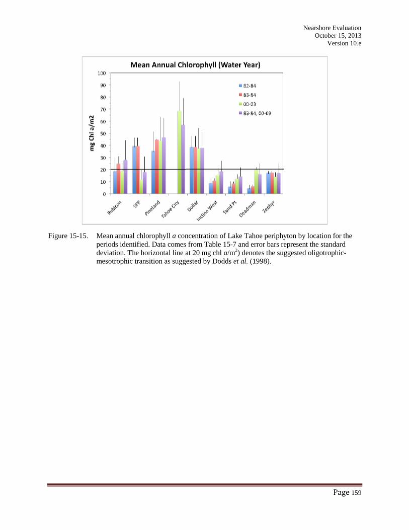
Nearshore Evaluation
October 15, 2013
Version 10.e
Page 159
Figure 15-15. Mean annual chlorophyll a concentration of Lake Tahoe periphyton by location for the
periods identified. Data comes from Table 15-7 and error bars represent the standard
deviation. The horizontal line at 20 mg chl a/m2) denotes the suggested oligotrophic-
mesotrophic transition as suggested by Dodds et al. (1998).
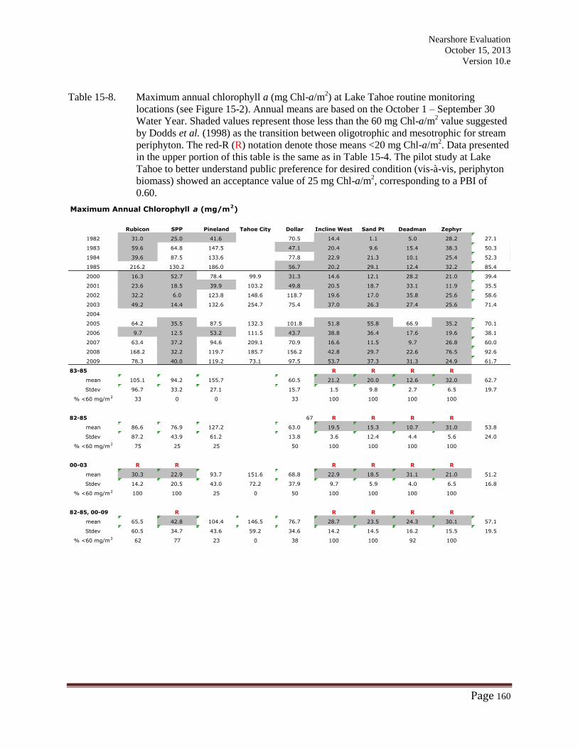
Nearshore Evaluation
October 15, 2013
Version 10.e
Page 160
Table 15-8. Maximum annual chlorophyll a (mg Chl-a/m2) at Lake Tahoe routine monitoring
locations (see Figure 15-2). Annual means are based on the October 1 – September 30
Water Year. Shaded values represent those less than the 60 mg Chl-a/m2 value suggested
by Dodds et al. (1998) as the transition between oligotrophic and mesotrophic for stream
periphyton. The red-R (R) notation denote those means <20 mg Chl-a/m2. Data presented
in the upper portion of this table is the same as in Table 15-4. The pilot study at Lake
Tahoe to better understand public preference for desired condition (vis-à-vis, periphyton
biomass) showed an acceptance value of 25 mg Chl-a/m2, corresponding to a PBI of
0.60.
Maximum Annual Chlorophyll a (mg/m2)
Rubicon SPP Pineland Tahoe City Dollar Incline West Sand Pt Deadman Zephyr
1982 31.0 25.0 41.6 70.5 14.4 1.1 5.0 28.2 27.1
1983 59.6 64.8 147.5 47.1 20.4 9.6 15.4 38.3 50.3
1984 39.6 87.5 133.6 77.8 22.9 21.3 10.1 25.4 52.3
1985 216.2 130.2 186.0 56.7 20.2 29.1 12.4 32.2 85.4
2000 16.3 52.7 78.4 99.9 31.3 14.6 12.1 28.2 21.0 39.4
2001 23.6 18.5 39.9 103.2 49.8 20.5 18.7 33.1 11.9 35.5
2002 32.2 6.0 123.8 148.6 118.7 19.6 17.0 35.8 25.6 58.6
2003 49.2 14.4 132.6 254.7 75.4 37.0 26.3 27.4 25.6 71.4
2004
2005 64.2 35.5 87.5 132.3 101.8 51.8 55.8 66.9 35.2 70.1
2006 9.7 12.5 53.2 111.5 43.7 38.8 36.4 17.6 19.6 38.1
2007 63.4 37.2 94.6 209.1 70.9 16.6 11.5 9.7 26.8 60.0
2008 168.2 32.2 119.7 185.7 156.2 42.8 29.7 22.6 76.5 92.6
2009 78.3 40.0 119.2 73.1 97.5 53.7 37.3 31.3 24.9 61.7
83-85 R R R R
mean 105.1 94.2 155.7 60.5 21.2 20.0 12.6 32.0 62.7
Stdev 96.7 33.2 27.1 15.7 1.5 9.8 2.7 6.5 19.7
% <60 mg/m2
33 0 0 33 100 100 100 100
82-85 67 R R R R
mean 86.6 76.9 127.2 63.0 19.5 15.3 10.7 31.0 53.8
Stdev 87.2 43.9 61.2 13.8 3.6 12.4 4.4 5.6 24.0
% <60 mg/m2
75 25 25 50 100 100 100 100
00-03 R R R R R R
mean 30.3 22.9 93.7 151.6 68.8 22.9 18.5 31.1 21.0 51.2
Stdev 14.2 20.5 43.0 72.2 37.9 9.7 5.9 4.0 6.5 16.8
% <60 mg/m2
100 100 25 0 50 100 100 100 100
82-85, 00-09 R R R R R
mean 65.5 42.8 104.4 146.5 76.7 28.7 23.5 24.3 30.1 57.1
Stdev 60.5 34.7 43.6 59.2 34.6 14.2 14.5 16.2 15.5 19.5
% <60 mg/m2
62 77 23 0 38 100 100 92 100
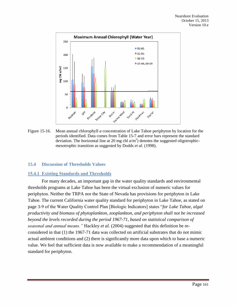
Nearshore Evaluation
October 15, 2013
Version 10.e
Page 161
Figure 15-16. Mean annual chlorophyll a concentration of Lake Tahoe periphyton by location for the
periods identified. Data comes from Table 15-7 and error bars represent the standard
deviation. The horizontal line at 20 mg chl a/m2) denotes the suggested oligotrophic-
mesotrophic transition as suggested by Dodds et al. (1998).
15.4 Discussion of Thresholds Values
15.4.1 Existing Standards and Thresholds
For many decades, an important gap in the water quality standards and environmental
thresholds programs at Lake Tahoe has been the virtual exclusion of numeric values for
periphyton. Neither the TRPA nor the State of Nevada has provisions for periphyton in Lake
Tahoe. The current California water quality standard for periphyton in Lake Tahoe, as stated on
page 3-9 of the Water Quality Control Plan [Biologic Indicators] states “for Lake Tahoe, algal
productivity and biomass of phytoplankton, zooplankton, and periphyton shall not be increased
beyond the levels recorded during the period 1967-71, based on statistical comparison of
seasonal and annual means.” Hackley et al. (2004) suggested that this definition be re-
considered in that (1) the 1967-71 data was collected on artificial substrates that do not mimic
actual ambient conditions and (2) there is significantly more data upon which to base a numeric
value. We feel that sufficient data is now available to make a recommendation of a meaningful
standard for periphyton.
Nearshore Evaluation
October 15, 2013
Version 10.e
Page 162
15.4.2 Approaches for Determining Standards and Thresholds
Numeric WQS exist in many forms – the most common are adoption of a single value
concentration for a selected parameter that cannot exceed a stated value and the annual average
(or some other indicator of average condition) that cannot exceed a stated value. Often, both are
adopted. In the case of open-water clarity at Lake Tahoe, this is fairly straight-forward; an
average annual value, measured at the long-term monitoring site is evaluated.
Water quality standards for periphyton can be developed by many means. For example,
(1) there may be a scientific literature which suggests that exceedence of a certain value would
be harmful to aquatic biota (e.g. toxics or dissolved oxygen), (2) numeric value(s) can be based
on either replicating conditions that existed some time in the past when water quality was in a
desirable condition or numerically defining current reference conditions (i.e. portions of the
water body not affected by pollutants), (3) statistically-based values using percentiles for
concentration (e.g. not to exceed 25 percent of the reference locationsb) or percentiles for
proportion the of shoreline that must be below a certain value (e.g. 80 percent of shore should be
less than 20 mg Chl a/m2)b (4) models can also be used to guide selection of values, and (5) in
the case of aesthetic beneficial uses, the selection of values can be based on the public/agency
perception of acceptable conditions. At this time there is no evidence to suggest that periphyton
growth is having a significant impact on lake biota. Consequently, a numeric WQS for
periphyton at Lake Tahoe would most likely be based on aesthetic concerns and/or the desire to
replicate previous conditions.
As discussed above, the accumulation/growth of periphyton biomass occurs on a number
of spatial and time scales. First, biomass can be evaluated as the amount/concentration of
material within a prescribed area (i.e. how much is present on a square meter of substrate – the
ability of a bottom surface to support biomass). Second, an indication of worsening conditions
could be that biomass is found during seasons when it historically did not occur. Third, growth
can increase based on the spatial extent of its distribution, even though the amount in an given
square meter may not of changed. The data collected to date primarily focuses on the first
scenario, i.e. the absolute amount of growth on a given area of substrate. This data is also good
for addressing the second point, i.e. extended temporal distribution. As presented below, there
are now five years where a full synoptic survey of biomass were monitored at 45-50 sites during
the period of the spring maxima.
The following looks at the applicability of these various approaches to deriving threshold
values for Tahoe periphyton.
Literature Definitions – The most widely cited reference for defining nuisance levels of
attached algae are those based on finding of researchers at the University of Washington
(Horner et al., 1983; Welch et al., 1988, 1989). Using chlorophyll a as a measure of
Nearshore Evaluation
October 15, 2013
Version 10.e
Page 163
biomass there authors suggested values on the order of 150-200 mg Chl a m-2
for a
maximum value and 100 mg Chl a m-2
for a mean value. Similarly, Suplee et al. (2009)
found that public opinion saw values >200 mg Chl a m-2
as undesirable for recreation. In
establishing guidelines for the Clark Fok River in Montana, the Tristate Implementation
Council (1996) used a values of 150 mg Chl a m-2
. British Columbia Environment
employ a value that is somewhat lower at 50-100 mg Chl a m-2
(Nordin 1985). However,
the goal for a periphyton abundance threshold in Lake Tahoe should not be established at
a nuisance level – it is too high. What is needed is a value more in-line with the
oligotrophic nature of this waterbody. Again from data collected in streams, Dodds et al.
(1998) recommended that the boundary between oligotrophic and mesotrophic be set at
20 mg Chl a m-2
for mean annual benthic chlorophyll and at 60 mg Chl a m-2
for
maximum benthic chlorophyll. These values are used in the U.S. EPA Nutrient Criteria
Technical Guidance Manual for Rivers and Streams (EPA 2000). The California
Watershed Assessment Manual also considered a value of 60 mg Chl a m-2
excessive in
cold water systems. The Virginia Water Resource Research Center (2006) published a
literature review for use in developing nutrient criteria in streams and rivers including a
discussion of work of Horner, Welch and others. All these values were developed for
stream periphyton and to our knowledge comparable values have not been published for
lake periphyton. In our opinion establishing a periphyton threshold for ultra-oligotrophic
Lake Tahoe based on a benchmark established for the oligotrophic-mesotrophic boundry
would also not be fully supportive of desired conditions.
Based on these findings, we do not believe that there is an adequate threshold value for
periphyton described in other systems that can be readily applied to Lake Tahoe.
Numeric Value(s) Based on Past, Existing or Desired Future Conditions – The current
State of California water quality standard for attached algae in Lake Tahoe is in the form
of a referral to past conditions. Unless current, existing conditions reflect desired
conditions and are in compliance with the Clean Water Act (or State) water quality
standards, the selection of existing conditions is usually not a recommended strategy.
When embarking on a strategy based on selecting past or future desired conditions as
water quality standards, it is very important that one’s expectations are realistic. While
we are not recommending a change to the beneficial use, as allowed under the Clean
Water Act4, caution needs to be applied so that it is not essentially impossible to ever
4 Under 40 CFR 131.10(g) states may remove a designated use which is not an existing use, as defined in § 131.3, or
establish sub-categories of a use if the State can demonstrate that attaining the designated use is not feasible. A Use
Attainability Analysis (UAA) is a structured scientific assessment of the factors affecting the attainment of uses
specified in Section 101(a)(2) of the Clean Water Act (the "fishable/swimmable" uses). The factors to be considered
in such an analysis include the physical, chemical, biological, and economic use removal criteria described in EPA' s
water quality standards regulation (40 CFR 131.10(g)(1)-(6)).
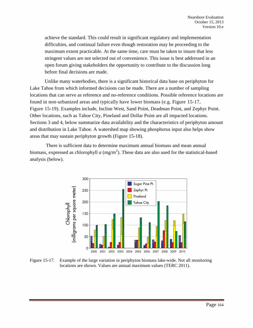
Nearshore Evaluation
October 15, 2013
Version 10.e
Page 164
achieve the standard. This could result in significant regulatory and implementation
difficulties, and continual failure even though restoration may be proceeding to the
maximum extent practicable. At the same time, care must be taken to insure that less
stringent values are not selected out of convenience. This issue is best addressed in an
open forum giving stakeholders the opportunity to contribute to the discussion long
before final decisions are made.
Unlike many waterbodies, there is a significant historical data base on periphyton for
Lake Tahoe from which informed decisions can be made. There are a number of sampling
locations that can serve as reference and no-reference conditions. Possible reference locations are
found in non-urbanized areas and typically have lower biomass (e.g. Figure 15-17,
Figure 15-19). Examples include, Incline West, Sand Point, Deadman Point, and Zephyr Point.
Other locations, such as Tahoe City, Pineland and Dollar Point are all impacted locations.
Sections 3 and 4, below summarize data availability and the characteristics of periphyton amount
and distribution in Lake Tahoe. A watershed map showing phosphorus input also helps show
areas that may sustain periphyton growth (Figure 15-18).
There is sufficient data to determine maximum annual biomass and mean annual
biomass, expressed as chlorophyll a (mg/m2). These data are also used for the statistical-based
analysis (below).
Figure 15-17. Example of the large variation in periphyton biomass lake-wide. Not all monitoring
locations are shown. Values are annual maximum values (TERC 2011).
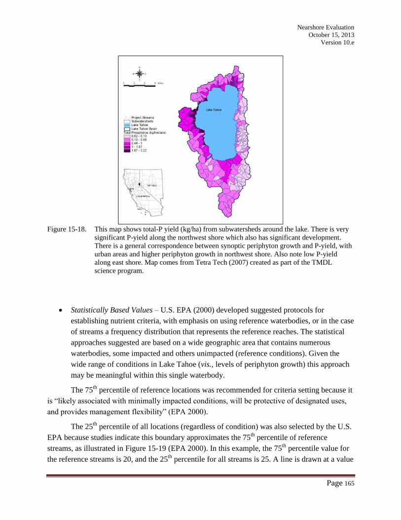
Nearshore Evaluation
October 15, 2013
Version 10.e
Page 165
Figure 15-18. This map shows total-P yield (kg/ha) from subwatersheds around the lake. There is very
significant P-yield along the northwest shore which also has significant development.
There is a general correspondence between synoptic periphyton growth and P-yield, with
urban areas and higher periphyton growth in northwest shore. Also note low P-yield
along east shore. Map comes from Tetra Tech (2007) created as part of the TMDL
science program.
Statistically Based Values – U.S. EPA (2000) developed suggested protocols for
establishing nutrient criteria, with emphasis on using reference waterbodies, or in the case
of streams a frequency distribution that represents the reference reaches. The statistical
approaches suggested are based on a wide geographic area that contains numerous
waterbodies, some impacted and others unimpacted (reference conditions). Given the
wide range of conditions in Lake Tahoe (vis., levels of periphyton growth) this approach
may be meaningful within this single waterbody.
The 75th
percentile of reference locations was recommended for criteria setting because it
is “likely associated with minimally impacted conditions, will be protective of designated uses,
and provides management flexibility” (EPA 2000).
The 25th
percentile of all locations (regardless of condition) was also selected by the U.S.
EPA because studies indicate this boundary approximates the 75th
percentile of reference
streams, as illustrated in Figure 15-19 (EPA 2000). In this example, the 75th
percentile value for
the reference streams is 20, and the 25th
percentile for all streams is 25. A line is drawn at a value
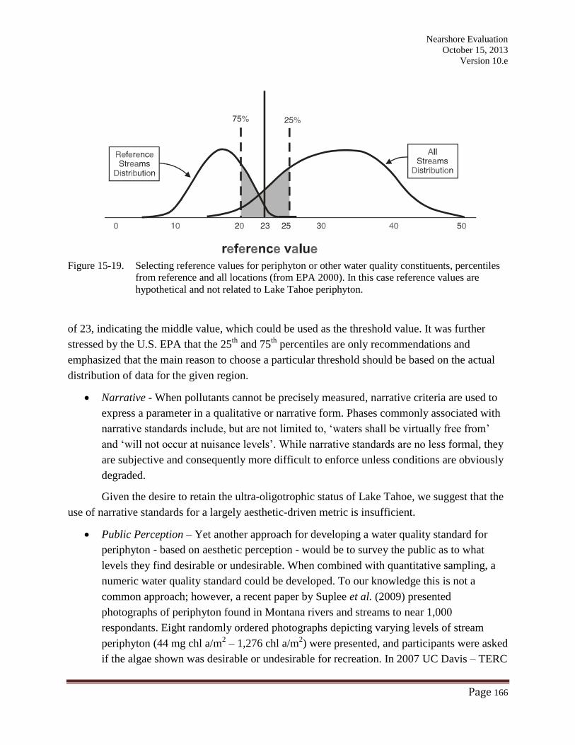
Nearshore Evaluation
October 15, 2013
Version 10.e
Page 166
Figure 15-19. Selecting reference values for periphyton or other water quality constituents, percentiles
from reference and all locations (from EPA 2000). In this case reference values are
hypothetical and not related to Lake Tahoe periphyton.
of 23, indicating the middle value, which could be used as the threshold value. It was further
stressed by the U.S. EPA that the 25th
and 75th
percentiles are only recommendations and
emphasized that the main reason to choose a particular threshold should be based on the actual
distribution of data for the given region.
Narrative - When pollutants cannot be precisely measured, narrative criteria are used to
express a parameter in a qualitative or narrative form. Phases commonly associated with
narrative standards include, but are not limited to, ‘waters shall be virtually free from’
and ‘will not occur at nuisance levels’. While narrative standards are no less formal, they
are subjective and consequently more difficult to enforce unless conditions are obviously
degraded.
Given the desire to retain the ultra-oligotrophic status of Lake Tahoe, we suggest that the
use of narrative standards for a largely aesthetic-driven metric is insufficient.
Public Perception – Yet another approach for developing a water quality standard for
periphyton - based on aesthetic perception - would be to survey the public as to what
levels they find desirable or undesirable. When combined with quantitative sampling, a
numeric water quality standard could be developed. To our knowledge this is not a
common approach; however, a recent paper by Suplee et al. (2009) presented
photographs of periphyton found in Montana rivers and streams to near 1,000
respondants. Eight randomly ordered photographs depicting varying levels of stream
periphyton (44 mg chl a/m2 – 1,276 chl a/m
2) were presented, and participants were asked
if the algae shown was desirable or undesirable for recreation. In 2007 UC Davis – TERC
Nearshore Evaluation
October 15, 2013
Version 10.e
Page 167
began a similar, unfunded, pilot study (see below). The use of public perception for
establishing legal water quality standards has advantages and disadvantages, and
regulatory agencies should carefully consider them all. For example, public desire is a
very common-sense approach for an aesthetic-based standard. However, public
perception can be subject to bias if a statistically-based design is not used to reach the
required cross-section human population. Ideally, the values obtained from the various
approaches discussed herein, will all focus on a narrow range of representative values.
Model Derived Values – According to Cattaneo et al. (1993), “periphyton is so highly
variable that is resists modeling.” While this is not to imply that valid periphyton models
do not exist or cannot be created, rather it highlights the hypothesis that the use of ‘off-
the shelf’ models developed elsewhere are not recommended for establishing formal
water quality standards. This is especially true for ultra-oligotrophic and oligotrophic
lakes. Since Lake Tahoe does not have a customized periphyton model, we suggest that
this approach (model-base standards) at this time would not be cost-effective or timely
enough approach for establishing standards for periphyton. However, in the future a
periphyton model could be extremely useful to evaluate management decisions related to
nutrient load reduction as has been the case with the Lake Clarity Model and the TMDL.
Using those stations and the 2000-2003 time period considered representative of
reference conditions, we developed a matrix of the various approaches for developing thresholds
as discussed in Section 2. Tables 15-9 and 15-10 summarizes the relevant cases for threshold
values that should be considered using mean annual biomass and maximum annual biomass
respectively. This analysis is intended to guide discussions between the water quality agencies
and the scientific community.
As part of a working hypothesis, we begin with the following points for consideration.
These points should form the basis for dialogue on actual recommended thresholds. Note that the
use of actual chlorophyll a concentration (mg/m2) is still an issue for active discussion. The
science team provides it here as an alternative for the reasons stated above. At this time the
mg/m2 and PBI can be interchanged based on the data and regression equation presented in
Figure 15-7 and future updates to this relationship.
1) In general, the threshold value should be very similar to the 20 mg chl a/m2 and
60 mg chl a/m2 suggested by Dodds et al. (1998) for mean annual biomass and
maximum annual biomass, respectively.

Nearshore Evaluation
October 15, 2013
Version 10.e
Page 168
Table 15-9. Matrix of approaches for developing periphyton biomass thresholds for Lake Tahoe
based on mean annual biomass. Biomass values for Lake Tahoe were measured as
chlorophyll a and converted to PBI based on the relation in Figure 15-10.
Mean Annual Biomass
Case Description Chlorophyll PBI Comments
(mg Chl a/m2)
12000-2003, mean of all
reference sites15.3 (3.4) 0.49 (0.31)
RP, SPP, IW, SP, DP, ZP. Mean of means
for six R-sites in Table 8.
22000-2003, mean+1stdev of
all reference sites20.3 (3.3) 0.49 (0.31)
RP, SPP, IW, SP, DP, ZP. Mean of means
for six R-sites in Table 8. RP and SPP
had elevated stdev relative to other
reference sites.
32000-2003, mean of all
reference sites+25%19.1 (4.3) 0.55 (0.32) see Case 3 comment
42000-2003, mean of west
shore reference sites15.2 (5.1) 0.49 (0.30) RP, SPP
52000-2003, mean+1stdev of
west shore reference sites22.7 (6.4) 0.60 (0.31) RP, SPP
62000-2003, mean of west
shore reference sites+25%19.0 (6.4) 0.54 (0.35) RP, SPP
72000-2003, mean of east
shore reference sites15.4 (3.2) 0.49 (0.30) IW, SP, DP, ZP
82000-2003, mean+1stdev of
east shore reference sites19.2 (2.8) 0.55 (0.30) IW, SP, DP, ZP
92000-2003, mean of east
shore reference sites+25%19.3 (3.3) 0.54 (0.26) IW, SP, DP, ZP
1075th percentile; all years; all
reference sites23.2 0.61
All years of record for RP, SPP, IW, SP,
DP, ZP. 10th percentile - 6.2 mg chl
a/m2, 25th - 9.6, 50th - 15.1, 75th -
23.2, 90 th - 32.7. USEPA guidance.
1125th percentile; all years; all
sites12.4 0.44
All years of record for RP, SPP, IW, SP,
DP, ZP, PL, TC, DP. 10th percentile - 7.3
mg chl a/m2, 25th - 12.4, 50th - 20.9,
75 th - 35.1, 90 th - 57.7. USEPA
guidance.
12Mean of 75th and 25 th
percentiles17.8 0.53 USEPA guidance.
13 Literature recommendation 20 0.56Oligotrophic-mesotrophic boundary
(Dodds et al. 1998)
14 Pilot Lake Tahoe Survey 25 0.60
Condition #3 in survey, level where
water contact would be avoided.
Acceptable conditions for Lake Tahoe
(condition #1 is - chl a = 14 and PBI =
0.47)
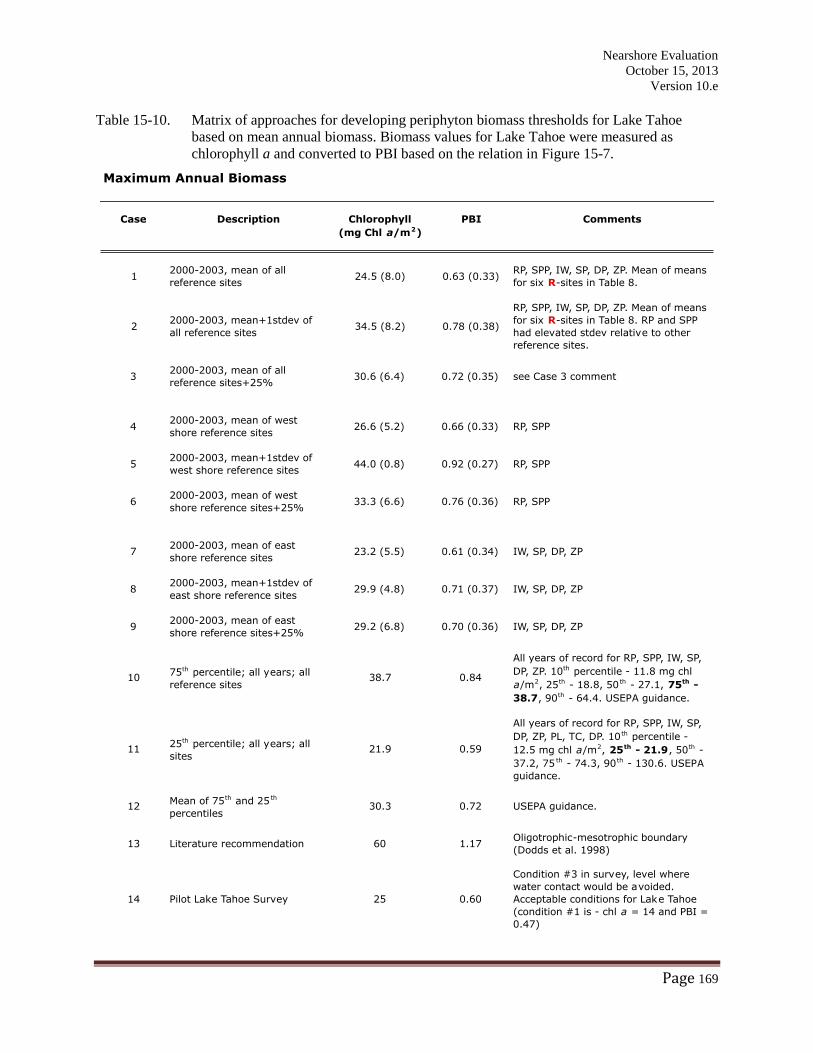
Nearshore Evaluation
October 15, 2013
Version 10.e
Page 169
Table 15-10. Matrix of approaches for developing periphyton biomass thresholds for Lake Tahoe
based on mean annual biomass. Biomass values for Lake Tahoe were measured as
chlorophyll a and converted to PBI based on the relation in Figure 15-7.
Maximum Annual Biomass
Case Description Chlorophyll PBI Comments
(mg Chl a/m2)
12000-2003, mean of all
reference sites24.5 (8.0) 0.63 (0.33)
RP, SPP, IW, SP, DP, ZP. Mean of means
for six R-sites in Table 8.
22000-2003, mean+1stdev of
all reference sites34.5 (8.2) 0.78 (0.38)
RP, SPP, IW, SP, DP, ZP. Mean of means
for six R-sites in Table 8. RP and SPP
had elevated stdev relative to other
reference sites.
32000-2003, mean of all
reference sites+25%30.6 (6.4) 0.72 (0.35) see Case 3 comment
42000-2003, mean of west
shore reference sites26.6 (5.2) 0.66 (0.33) RP, SPP
52000-2003, mean+1stdev of
west shore reference sites44.0 (0.8) 0.92 (0.27) RP, SPP
62000-2003, mean of west
shore reference sites+25%33.3 (6.6) 0.76 (0.36) RP, SPP
72000-2003, mean of east
shore reference sites23.2 (5.5) 0.61 (0.34) IW, SP, DP, ZP
82000-2003, mean+1stdev of
east shore reference sites29.9 (4.8) 0.71 (0.37) IW, SP, DP, ZP
92000-2003, mean of east
shore reference sites+25%29.2 (6.8) 0.70 (0.36) IW, SP, DP, ZP
1075th percentile; all years; all
reference sites38.7 0.84
All years of record for RP, SPP, IW, SP,
DP, ZP. 10th percentile - 11.8 mg chl
a/m2, 25th - 18.8, 50 th - 27.1, 75th -
38.7, 90th - 64.4. USEPA guidance.
1125th percentile; all years; all
sites21.9 0.59
All years of record for RP, SPP, IW, SP,
DP, ZP, PL, TC, DP. 10th percentile -
12.5 mg chl a/m2, 25th - 21.9, 50th -
37.2, 75 th - 74.3, 90th - 130.6. USEPA
guidance.
12Mean of 75th and 25 th
percentiles30.3 0.72 USEPA guidance.
13 Literature recommendation 60 1.17Oligotrophic-mesotrophic boundary
(Dodds et al. 1998)
14 Pilot Lake Tahoe Survey 25 0.60
Condition #3 in survey, level where
water contact would be avoided.
Acceptable conditions for Lake Tahoe
(condition #1 is - chl a = 14 and PBI =
0.47)
Nearshore Evaluation
October 15, 2013
Version 10.e
Page 170
2) The use of reference conditions is a reasonable and defendable strategy. However, as
indicated by biomass conditions at Pineland, Tahoe City and other locations around
the Lake, it is expected that significant nutrient reduction actions would be required
for these locations to be in compliance (i.e. reflect reference conditions). In many
areas we suspect that a targeted load reduction effort as part of the TMDL would help
reduce periphyton biomass. In other areas, such as Rubicon Point (e.g., 1983, 1985,
2007-2009) and Sugar Pine Point (e.g. 1982-1985), biomass can be high despite the
fact that these west shore locations are located in undeveloped areas. That is,
periphyton biomass can sometimes be high with no apparent nutrient source (see
discussion in Cattaneo et al., 1993). Accommodations need to be make for this
phenomenon, but not at the expense of protection elsewhere (i.e. increasing a
threshold value to accommodate these areas).
3) Lake level can have a large affect on apparent periphyton biomass. With a low lake
level, associated with multiple dry years, the cyanobacterial dominated sublittoral
periphyton community is located higher in the water column than usual. Sampling at
the standard 0.5 m depth will artificially result in an increase in biomass. Previous
studies has shown the use of artificial plates or other substrata to be ineffective in
adequately mimicking the eulittoral zone in Lake Tahoe (Aloi 1988; Aloi et al.,
1988). A threshold would need to accommodate this phenomenon.
4) Considering the six sites identified as reference locations in Section 5 above (RP,
SPP, IW, SP, DP, ZP) for the period 2000-2003, there is general agreement between
the various cases presented in Table 15-9 for mean annual biomass. Case 1 represents
the mean of all these sites at 15.3±3.4 mg chl a/m2. This value increases to
approximately 20 mg chl a/m2 when a margin of one standard deviation or
+25 percent is applied. Very similar values were obtained when the west shore and
east shore reference sites were separated. The mean of the 25th
and 75th
percentiles
was also similar at a value of 17.8 mg chl a/m2 (Table 15-9). The pilot Lake Tahoe
public perception survey resulted in a value of 25 mg chl a/m2; however, a distinction
between mean annual and maximum annual biomass was not made. This range is also
very close to the 20 mg chl a/m2 suggested by Dodds et al. (1998).
Based on these data, a threshold for mean annual periphyton biomass in the range of
17.5-22.5 mg chl a/m2 (PBI = 0.52-0.60) would not be an unreasonable starting point for
discussion.
5) For maximum annual biomass, the mean of all six references sites was 24.5±8.0 mg
chl a/m2 (Table 15-10). When a margin of one standard deviation or +25 percent is
applied to value increased to 30-35 chl a/m2. The mean for maximum annual biomass
was very similar when the west and east shore reference sites were separated
Nearshore Evaluation
October 15, 2013
Version 10.e
Page 171
(23.2±5.5 chl a/m2
and 26.6 chl a/m2, respectively). The one standard deviation and
+25 percent margins were, 44.0±0.8 and 33.3±6.6 chl a/m2, respectively for the west
shore reference sites and 29.9±4.8 chl a/m2 and 29.2±6.8 chl a/m
2, respectively for
the east shore reference sites (Table 810). The higher values for one standard
deviation for the west shore sites reflects more variable interannual differences in
periphyton biomass (note, this is touched on in point (2) just above. The mean of the
25th
and 75th
percentiles is 30.3 chl a/m2 while the pilot Lake Tahoe survey indicated
a desirable condition at 25 chl a/m2. These values are all lower than the 60 chl a/m
2
suggested by Dodds et al. (1998).
Based on these data, a threshold for maximum annual periphyton biomass in the range of
25-35 mg chl a/m2 (PBI = 0.64-0.79) would not be an unreasonable starting point for discussion.
In general terms, and using the chlorophyll-PBI conversion, on the order of 35-40 percent of the
lake shore exceed this range in 2008, 2009 and 2010, while 50-55 percent exceeded it in 2011
(refer to Figure 15-11).
15.5 Metric Monitoring Plan
The 116 km shoreline of Lake Tahoe is characterized by extensive areas of steep
gradient, large boulders separating regions of shallow gradient cobble and sand. Generally, land
areas with steep slopes are less developed and are often contained within state park or national
forest service boundaries. The land associated with more gently sloping shorelines tends to
support development including roadways. Residential neighborhoods surrounding the urban
landscape often spread to the edge of undeveloped forest lands, creating zones of moderate
development. To adequately represent the range of shorezone conditions, nine periphyton
sampling locations have been established around the lake located on the north, east and west
shores (Hackley, 2011). The south shore consists primarily of a sand bottom and was not
included in the epilithic (rocks) monitoring.
15.5.1 Routine Monitoring
Nine routine stations are shown in the map for monitoring locations (Figure 15-2). Their
coordinates and associated level of watershed development are given in Table 15-11. These nine
sites represent a range of backshore disturbance levels from relatively undisturbed land (Rubicon
Point and Deadman Point) to a developed urban center (Tahoe City). Except for Tahoe City these
sites were used in the 1982-1985 surveys. Since 2000, all the sites in Table 15-11 have been used
for periphyton monitoring. We recommend a continuation of these sites for the routine
monitoring during the year. They cover a wide range of development levels and have an
extensive historical data based for evaluating long-term trends.
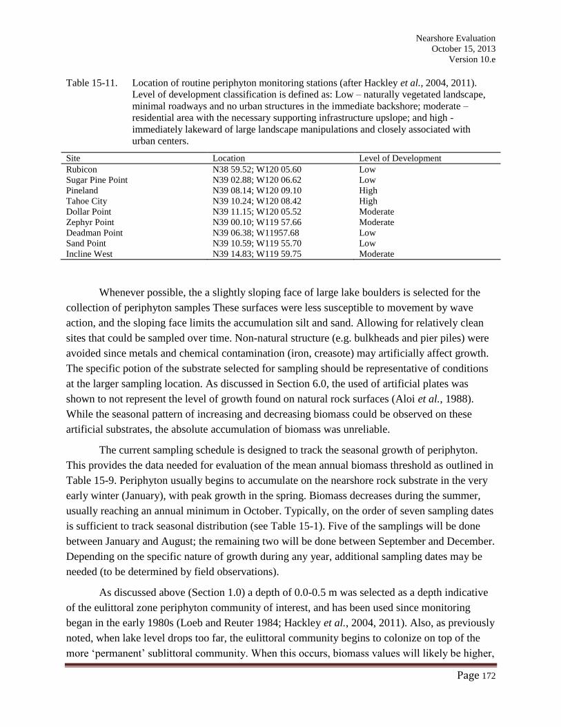
Nearshore Evaluation
October 15, 2013
Version 10.e
Page 172
Table 15-11. Location of routine periphyton monitoring stations (after Hackley et al., 2004, 2011).
Level of development classification is defined as: Low – naturally vegetated landscape,
minimal roadways and no urban structures in the immediate backshore; moderate –
residential area with the necessary supporting infrastructure upslope; and high -
immediately lakeward of large landscape manipulations and closely associated with
urban centers.
Site Location Level of Development
Rubicon
Sugar Pine Point
Pineland
Tahoe City
Dollar Point
Zephyr Point
Deadman Point
Sand Point
Incline West
N38 59.52; W120 05.60
N39 02.88; W120 06.62
N39 08.14; W120 09.10
N39 10.24; W120 08.42
N39 11.15; W120 05.52
N39 00.10; W119 57.66
N39 06.38; W11957.68
N39 10.59; W119 55.70
N39 14.83; W119 59.75
Low
Low
High
High
Moderate
Moderate
Low
Low
Moderate
Whenever possible, the a slightly sloping face of large lake boulders is selected for the
collection of periphyton samples These surfaces were less susceptible to movement by wave
action, and the sloping face limits the accumulation silt and sand. Allowing for relatively clean
sites that could be sampled over time. Non-natural structure (e.g. bulkheads and pier piles) were
avoided since metals and chemical contamination (iron, creasote) may artificially affect growth.
The specific potion of the substrate selected for sampling should be representative of conditions
at the larger sampling location. As discussed in Section 6.0, the used of artificial plates was
shown to not represent the level of growth found on natural rock surfaces (Aloi et al., 1988).
While the seasonal pattern of increasing and decreasing biomass could be observed on these
artificial substrates, the absolute accumulation of biomass was unreliable.
The current sampling schedule is designed to track the seasonal growth of periphyton.
This provides the data needed for evaluation of the mean annual biomass threshold as outlined in
Table 15-9. Periphyton usually begins to accumulate on the nearshore rock substrate in the very
early winter (January), with peak growth in the spring. Biomass decreases during the summer,
usually reaching an annual minimum in October. Typically, on the order of seven sampling dates
is sufficient to track seasonal distribution (see Table 15-1). Five of the samplings will be done
between January and August; the remaining two will be done between September and December.
Depending on the specific nature of growth during any year, additional sampling dates may be
needed (to be determined by field observations).
As discussed above (Section 1.0) a depth of 0.0-0.5 m was selected as a depth indicative
of the eulittoral zone periphyton community of interest, and has been used since monitoring
began in the early 1980s (Loeb and Reuter 1984; Hackley et al., 2004, 2011). Also, as previously
noted, when lake level drops too far, the eulittoral community begins to colonize on top of the
more ‘permanent’ sublittoral community. When this occurs, biomass values will likely be higher,
Nearshore Evaluation
October 15, 2013
Version 10.e
Page 173
making time series analysis more difficult. Careful notation is needed to document lake level and
location of the sublittoral biomass for each sampling, especially during periods of dry years.
Samples are typically collected by snorkeling and therefore all required health and safety
precautions should be in place and strictly followed. Two-syringe samplers are used to remove
and collect periphyton from a known surface area of 5.3 cm (Loeb 1981). All historic data from
the early 1980s onward have been done using this technique (Hackley et al., 2004 et seq.). Stage
one of the syringe containing the brush is placed over the area to be sampled. The brush is turned
several times to remove the biomass from the surface. Loosened periphyton in the brushing
syringe is then collected by withdrawing the plunger of the second stage syringe. The end of
stage one is then corked, the sampler is brought to the surface and placed into an ice chest and
returned to the laboratory for processing on the same day. Duplicate samples are taken.
However, if the researcher determines, in the field, that there is a high degree of heterogeneity
(based on experience and best professional judgment), triplicate samples are collected.
Upon returned to the laboratory, water and periphyton are removed from the sampler,
centrifuged to separate water and concentrate biomass. The water is decanted off and the
concentrated biomass is transferred to a pre-tared filter and weighed. A known (weighed)
subsample is then removed and frozen for later chlorophyll a analysis. The remaining biomass
can be used for species identification of other assays if so desired. Processing and analytical
methods are described in Loeb and Reuter and summarized in Hackley et al. (2004).
Chlorophyll a is analyzed using a hot methanol extraction. Samples (frozen until
analysis) are mixed and ground with a glass rod in the boiling methanol, under a fume hood for
approximately three minutes. The solution is centrifuged to remove turbidity. Absorbances of the
supernatant are immediately measured using a spectrophotometer at wavelengths of 750, 666 and
653 nm. The chlorophyll a content is determined using the equation of Iwamura et al. (1970):
Chlorophyll a (mg/m2) = (17.12 * Abs666 – 8.68 * Abs653) * (Methanol Volume (mL) * Total Sample Wet
Weight (g)) ÷ (4 (cm) * Chlorophyll a Subsample Wet Weight (g) * 5.3*10-4 (m2))/1000
Standard reference material (SRM) with known concentrations of chlorophyll a, are used
at least annually to calibrate the spectrophotometer and extraction procedures. The quality
control procedure (Hackley et al., 2004) require analytical calibration of the laboratory
instrumentation and field equipment including, snorkeling gear, two-syringe samplers, analytical
balance and spectrophotometer.
All field measurements and observations will be recorded at the time of sampling using a
standardized field form or field notebook. Field observations for biomass percent cover and
length are converted to PBI values. Chlorophyll a and biomass will are entered on a standardized
periphyton laboratory data sheet. All data will be entered into a database developed specifically
for this program.
Nearshore Evaluation
October 15, 2013
Version 10.e
Page 174
Annual reports should contain (at a minimum):
Tables with current year data (reflecting the October 1 – September 3 water year)
Placement of current year data on to plots containing long-term data for (1) chlorophyll a
on each collection date, (2) mean annual biomass (over the water year, (maximum annual
biomass), (3) tables and graphs for synoptic PBI data
Time-series analysis using each chlorophyll a data point for each station using the Mann-
Kendall or another appropriate statistical test.
Update of chlorophyll a versus PBI relationships
Plots of percent lake shoreline versus PBI (for synoptic, spring sampling)
Comparison to threshold values
15.5.2 Synoptic – Maximum Biomass Monitoring
While the nine routine sampling sites provide data from a wide range of conditions
around the lake (low to high development) during a full annual cycle, the limited number of
these sites does not provide enough spatial resolution to determine periphyton biomass on a
whole-lake scale. For this reason, the current monitoring program includes synoptic sampling,
once a year, at approximately 40 sites (see Figure 5) monitored for biomass accumulation along
with the nine routine sites discussed above. This synoptic monitoring is timed as much as
possible to correspond to peak periphyton growth in each region of the lake, and which typically
occurs in the spring. It is important to note that the peak annual biomass does not occur
simultaneously around the entire lake, with certain areas reaching peak levels sooner or later than
others. To make the whole-lake data comparable, the specific timing for this type of sampling
coordinated with conditions in the field. Table 15-12 presents the names and locations of these
synoptic sites. This monitoring provides the data needed to evaluate the maximum annual
biomass threshold(s) as presented in Table 15-10.
Each of these synoptic sites is monitored visually while snorkeling. Measurements of
filament length, percent bottom coverage, and observations on main algal types present are
made. Data on filament length and percent bottom coverage is used to calculate the Periphyton
Biomass Index (PBI) as first discussed in Section 4.2. Below water photographs should be taken
at each site.
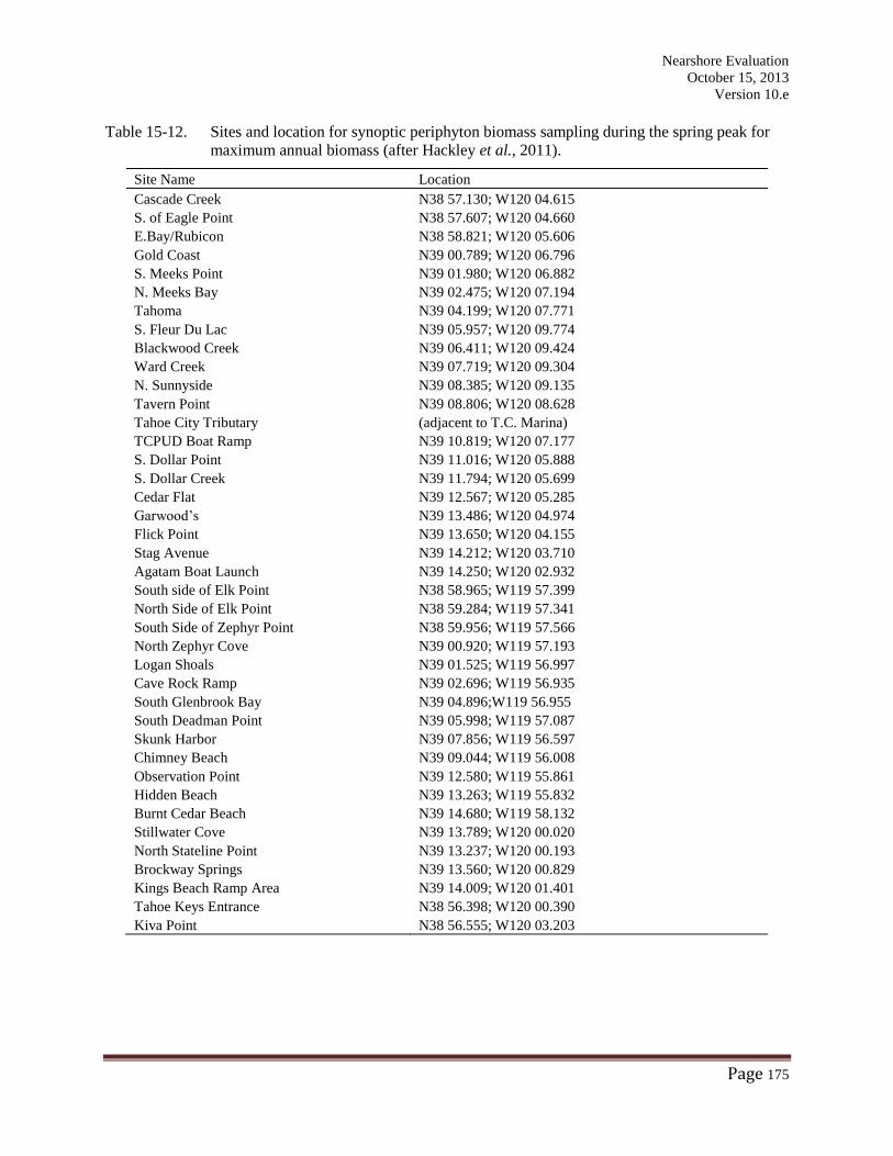
Nearshore Evaluation
October 15, 2013
Version 10.e
Page 175
Table 15-12. Sites and location for synoptic periphyton biomass sampling during the spring peak for
maximum annual biomass (after Hackley et al., 2011).
Site Name Location
Cascade Creek N38 57.130; W120 04.615
S. of Eagle Point N38 57.607; W120 04.660
E.Bay/Rubicon N38 58.821; W120 05.606
Gold Coast N39 00.789; W120 06.796
S. Meeks Point N39 01.980; W120 06.882
N. Meeks Bay N39 02.475; W120 07.194
Tahoma N39 04.199; W120 07.771
S. Fleur Du Lac N39 05.957; W120 09.774
Blackwood Creek N39 06.411; W120 09.424
Ward Creek N39 07.719; W120 09.304
N. Sunnyside N39 08.385; W120 09.135
Tavern Point N39 08.806; W120 08.628
Tahoe City Tributary (adjacent to T.C. Marina)
TCPUD Boat Ramp N39 10.819; W120 07.177
S. Dollar Point N39 11.016; W120 05.888
S. Dollar Creek N39 11.794; W120 05.699
Cedar Flat N39 12.567; W120 05.285
Garwood’s N39 13.486; W120 04.974
Flick Point N39 13.650; W120 04.155
Stag Avenue N39 14.212; W120 03.710
Agatam Boat Launch N39 14.250; W120 02.932
South side of Elk Point N38 58.965; W119 57.399
North Side of Elk Point N38 59.284; W119 57.341
South Side of Zephyr Point N38 59.956; W119 57.566
North Zephyr Cove N39 00.920; W119 57.193
Logan Shoals N39 01.525; W119 56.997
Cave Rock Ramp N39 02.696; W119 56.935
South Glenbrook Bay N39 04.896;W119 56.955
South Deadman Point N39 05.998; W119 57.087
Skunk Harbor N39 07.856; W119 56.597
Chimney Beach N39 09.044; W119 56.008
Observation Point N39 12.580; W119 55.861
Hidden Beach N39 13.263; W119 55.832
Burnt Cedar Beach N39 14.680; W119 58.132
Stillwater Cove N39 13.789; W120 00.020
North Stateline Point N39 13.237; W120 00.193
Brockway Springs N39 13.560; W120 00.829
Kings Beach Ramp Area N39 14.009; W120 01.401
Tahoe Keys Entrance N38 56.398; W120 00.390
Kiva Point N38 56.555; W120 03.203
Nearshore Evaluation
October 15, 2013
Version 10.e
Page 176
PBI is calculated by multiplying the filament length (cm) times the ratio of substrate area
covered with algae. Typically, this observation is made within a 25 m2
area. For example, if
80 percent of the area is covered with periphyton 1 cm in thickness the PBI would be
0.80*1.0 = 0.80 PBI units.
It is important that the routine sampling (Section 9.5.1) during the period of the spring
biomass maximum be done in association with this synoptic sampling. In this way, the
measurements for PBI and chlorophyll can be taken as close together in time as possible. These
data should then be used to update/revise the Chl a/PBI relationship as seen in Figure 15-7.
16.0 MACROPHYTES
During the 1920’s and 1930’s the Mt. Ralston Fish Planting Club released invertebrates,
fishes, and stocked aquatic plants such as water lilies, water hyacinth, and parrot feather into the
numerous higher elevation lakes, likely including the Tahoe basin. The intentional introductions
were meant to improve food and cover conditions for fishes in the generally rocky and sandy
bottom waters. It is likely the stocking of plants also continued until the 1950’s as biologist,
Shebley, from the California Fish and Game indicated that they were introducing invertebrates
such as salmon flies, gammarus, and aquatic plants but he didn’t specify the taxa. As late as
1961, Nevada Fish and Game introduced Vallisneria (likely water celery, V. Americana) into the
lake in an effort to improve fish and cover conditions in the lake. Thirty plants were anchored to
the bottom in 1-1.75 m of water at 3 locations (Skunk Harbon, Glenbrook Bay, and Logan
shoals) but they did not establish.
16.1 History of Metric Monitoring
Lake Tahoe’s nearshore area contains few aquatic plants with the exception of a native
water milfoil species and Elodea Canadensis. The Eurasian watermilfoil (Myriolphyllum
spicatum) is the main invasive plant to establish in Lake Tahoe. Native to Eurasia and Northern
Africa, the plant was introduced into North American many decades ago and has spread
throughout the continent through boater activity and possibly by waterbirds. The plant fragments,
and propagules of the fragments can colonize and grow when attached to substrate. To date many
locations of this nonnative plants are largely within marinas, closed embayments, or waters
where there is little physical mixing (e.g. West end of Emerald Bay). There are however open
water sites on the West shore likely resulting from the anchoring of boat anchors or pier
construction equipment. A study by Walter (2000) surmised the plant was introduced into the
Tahoe Keys and that creation of plant fragments due to harvesting and control efforts by the
Tahoe Keys Homeowner Association with subsequent movement by boats or exchange of
currents with the main lake has led to new populations establishing around the lake. In 2003, a
more aggressive plant was noted in the Tahoe Keys. Curly leaf pondweed (Potomageton crispus)
can colonize open water areas and is rapidly moving to new locations in the South Shore.