Embed Size (px)
Citation preview
425
Copyright © 2015 by Roland Stull. Practical Meteorology: An Algebra-based Survey of Atmospheric Science
13 Extratropical cyclonEs
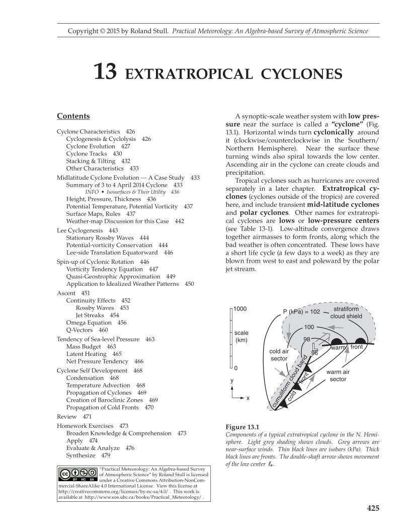
A synoptic-scale weather system with low pres-sure near the surface is called a “cyclone” (Fig. 13.1). Horizontal winds turn cyclonically around it (clockwise/counterclockwise in the Southern/Northern Hemisphere). Near the surface these turning winds also spiral towards the low center. Ascending air in the cyclone can create clouds and precipitation. Tropical cyclones such as hurricanes are covered separately in a later chapter. Extratropical cy-clones (cyclones outside of the tropics) are covered here, and include transient mid-latitude cyclones and polar cyclones. Other names for extratropi-cal cyclones are lows or low-pressure centers (see Table 13-1). Low-altitude convergence draws together airmasses to form fronts, along which the bad weather is often concentrated. These lows have a short life cycle (a few days to a week) as they are blown from west to east and poleward by the polar jet stream.
contents
Cyclone Characteristics 426Cyclogenesis & Cyclolysis 426Cyclone Evolution 427Cyclone Tracks 430Stacking & Tilting 432Other Characteristics 433
Midlatitude Cyclone Evolution — A Case Study 433Summary of 3 to 4 April 2014 Cyclone 433
INFO • Isosurfaces & Their Utility 436Height, Pressure, Thickness 436Potential Temperature, Potential Vorticity 437Surface Maps, Rules 437Weather-map Discussion for this Case 442
Lee Cyclogenesis 443Stationary Rossby Waves 444Potential-vorticity Conservation 444Lee-side Translation Equatorward 446
Spin-up of Cyclonic Rotation 446Vorticity Tendency Equation 447Quasi-Geostrophic Approximation 449Application to Idealized Weather Patterns 450
Ascent 451Continuity Effects 452
Rossby Waves 453Jet Streaks 454
Omega Equation 456Q-Vectors 460
Tendency of Sea-level Pressure 463Mass Budget 463Latent Heating 465Net Pressure Tendency 466
Cyclone Self Development 468Condensation 468Temperature Advection 468Propagation of Cyclones 469Creation of Baroclinic Zones 469Propagation of Cold Fronts 470
Review 471
Homework Exercises 473Broaden Knowledge & Comprehension 473Apply 474Evaluate & Analyze 476Synthesize 479
Figure 13.1Components of a typical extratropical cyclone in the N. Hemi-sphere. Light grey shading shows clouds. Grey arrows are near-surface winds. Thin black lines are isobars (kPa). Thick black lines are fronts. The double-shaft arrow shows movement of the low center L .
“Practical Meteorology: An Algebra-based Survey of Atmospheric Science” by Roland Stull is licensed under a Creative Commons Attribution-NonCom-
mercial-ShareAlike 4.0 International License. View this license at http://creativecommons.org/licenses/by-nc-sa/4.0/ . This work is available at http://www.eos.ubc.ca/books/Practical_Meteorology/ .
426 chaptEr 13 • Extratropical cyclonEs
CyClone CharaCteristiCs
Cyclogenesis & Cyclolysis Cyclones are born and intensify (cyclogenesis) and later weaken and die (cyclolysis). During cy-clogenesis the (1) vorticity (horizontal winds turn-ing around the low center) and (2) updrafts (vertical winds) increase while the (3) surface pressure de-creases. The intertwined processes that control these three characteristics will be the focus of three major sections in this chapter. In a nutshell, updrafts over a synoptic-scale region remove air from near the surface, causing the air pressure to decrease. The pressure gradient between this low-pressure cen-ter and the surroundings drives horizontal winds, which are forced to turn because of Coriolis force. Frictional drag near the ground causes these winds to spiral in towards the low center, adding more air molecules horizontally to compensate for those be-ing removed vertically. If the updraft weakens, the inward spiral of air molecules fills the low to make it less low (cyclolysis). Cyclogenesis is enhanced at locations where one or more of the following conditions occur:
(1) east of mountain ranges, where terrain slopes downhill under the jet stream.
(2) east of deep troughs (and west of strong ridges) in the polar jet stream, where horizontal divergence of winds drives mid-tropospheric updrafts.
(3) at frontal zones or other baroclinic regions where horizontal temperature gradients are large.
(4) at locations that don’t suppress vertical motions, such as where static stability is weak.
(5) where cold air moves over warm, wet surfaces such as the Gulf Stream, such that strong evapo-ration adds water vapor to the air and strong sur-face heating destabilizes the atmosphere.
(6) at locations further from the equator, where Coriolis force is greater.
If cyclogenesis is rapid enough (central pressures dropping 2.4 kPa or more over a 24-hour period), the process is called explosive cyclogenesis (also nicknamed a cyclone bomb). This can occur when multiple conditions listed above are occurring at the same location (such as when a front stalls over the Gulf Stream, with a strong amplitude Rossby-wave trough to the west). During winter, such cy-clone bombs can cause intense cyclones just off the east coast of the USA with storm-force winds, high waves, and blizzards or freezing rain.
table 13-1. Cyclone names. “Core” is storm center. T is relative temperature.
common name inn. amer.
Formalname
other common
names
t of the
core
Mapsym-bol
lowextra-
tropicalcyclone
mid-latitudecyclone
cold Llow-pressure
centerstorm system*
cyclone(in N. America)
hurricanetropicalcyclone
typhoon(in W. Pacific)
warmcyclone
(in Australia)
(* Often used by TV meteorologists.)
inFo • southern hemisphere lows
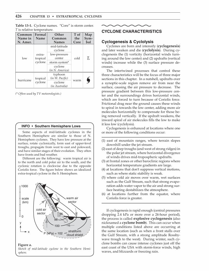
Some aspects of mid-latitude cyclones in the Southern Hemisphere are similar to those of N. Hemisphere cyclones. They have low pressure at the surface, rotate cyclonically, form east of upper-level troughs, propagate from west to east and poleward, and have similar stages of their evolution. They often have fronts and bad weather. Different are the following: warm tropical air is to the north and cold polar air to the south, and the cyclonic rotation is clockwise due to the opposite Coriolis force. The figure below shows an idealized extra-tropical cyclone in the S. Hemisphere.
Figure a.Sketch of mid-latitude cyclone in the Southern Hemi-sphere.
r. stull • practical MEtEorology 427
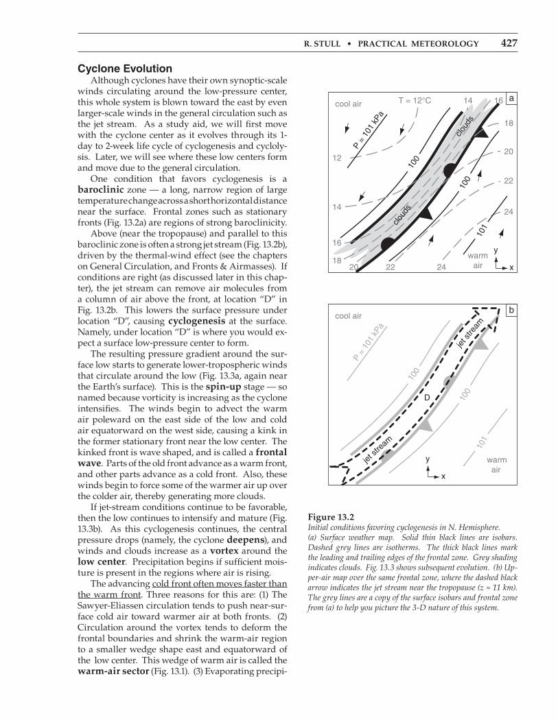
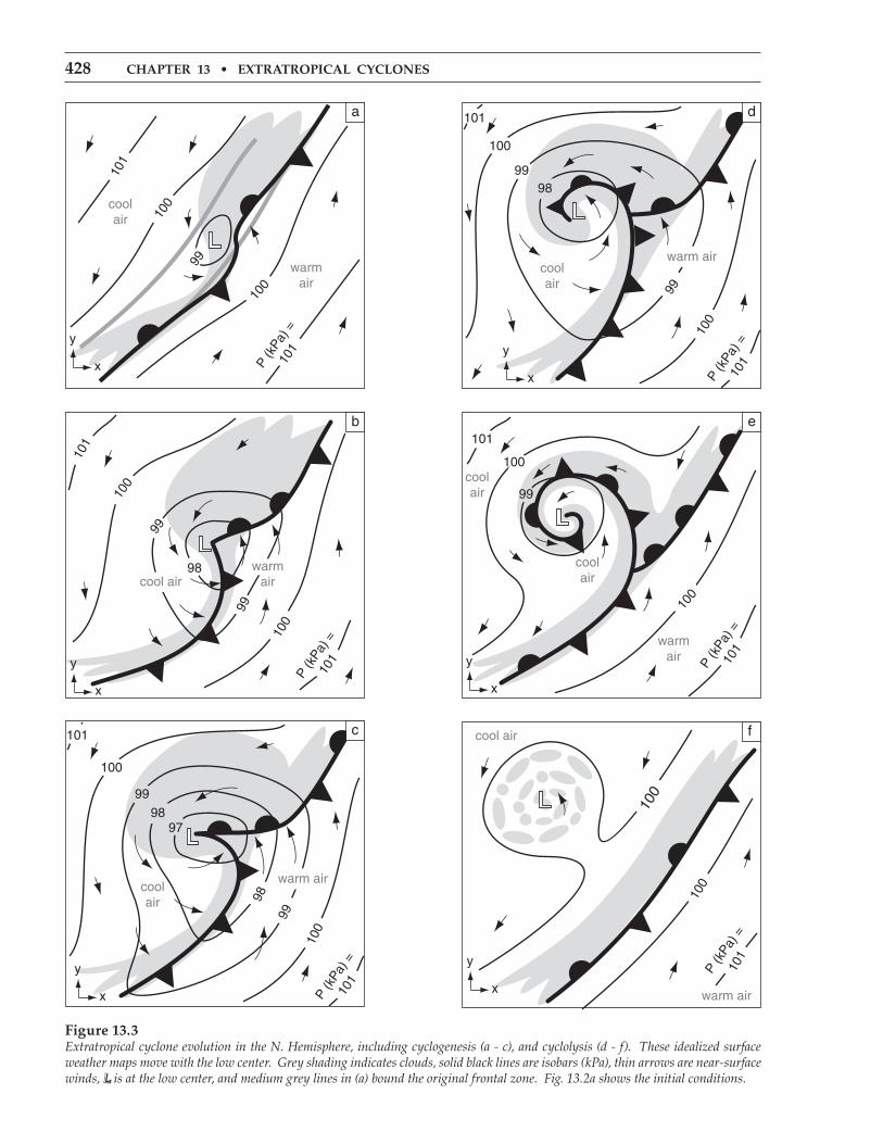
Cyclone evolution Although cyclones have their own synoptic-scale winds circulating around the low-pressure center, this whole system is blown toward the east by even larger-scale winds in the general circulation such as the jet stream. As a study aid, we will first move with the cyclone center as it evolves through its 1-day to 2-week life cycle of cyclogenesis and cycloly-sis. Later, we will see where these low centers form and move due to the general circulation. One condition that favors cyclogenesis is a baroclinic zone — a long, narrow region of large temperature change across a short horizontal distance near the surface. Frontal zones such as stationary fronts (Fig. 13.2a) are regions of strong baroclinicity. Above (near the tropopause) and parallel to this baroclinic zone is often a strong jet stream (Fig. 13.2b), driven by the thermal-wind effect (see the chapters on General Circulation, and Fronts & Airmasses). If conditions are right (as discussed later in this chap-ter), the jet stream can remove air molecules from a column of air above the front, at location “D” in Fig. 13.2b. This lowers the surface pressure under location “D”, causing cyclogenesis at the surface. Namely, under location “D” is where you would ex-pect a surface low-pressure center to form. The resulting pressure gradient around the sur-face low starts to generate lower-tropospheric winds that circulate around the low (Fig. 13.3a, again near the Earth’s surface). This is the spin-up stage — so named because vorticity is increasing as the cyclone intensifies. The winds begin to advect the warm air poleward on the east side of the low and cold air equatorward on the west side, causing a kink in the former stationary front near the low center. The kinked front is wave shaped, and is called a frontal wave. Parts of the old front advance as a warm front, and other parts advance as a cold front. Also, these winds begin to force some of the warmer air up over the colder air, thereby generating more clouds. If jet-stream conditions continue to be favorable, then the low continues to intensify and mature (Fig. 13.3b). As this cyclogenesis continues, the central pressure drops (namely, the cyclone deepens), and winds and clouds increase as a vortex around the low center. Precipitation begins if sufficient mois-ture is present in the regions where air is rising. The advancing cold front often moves faster than the warm front. Three reasons for this are: (1) The Sawyer-Eliassen circulation tends to push near-sur-face cold air toward warmer air at both fronts. (2) Circulation around the vortex tends to deform the frontal boundaries and shrink the warm-air region to a smaller wedge shape east and equatorward of the low center. This wedge of warm air is called the warm-air sector (Fig. 13.1). (3) Evaporating precipi-
Figure 13.2Initial conditions favoring cyclogenesis in N. Hemisphere. (a) Surface weather map. Solid thin black lines are isobars. Dashed grey lines are isotherms. The thick black lines mark the leading and trailing edges of the frontal zone. Grey shading indicates clouds. Fig. 13.3 shows subsequent evolution. (b) Up-per-air map over the same frontal zone, where the dashed black arrow indicates the jet stream near the tropopause (z ≈ 11 km). The grey lines are a copy of the surface isobars and frontal zone from (a) to help you picture the 3-D nature of this system.
428 chaptEr 13 • Extratropical cyclonEs
Figure 13.3Extratropical cyclone evolution in the N. Hemisphere, including cyclogenesis (a - c), and cyclolysis (d - f). These idealized surface weather maps move with the low center. Grey shading indicates clouds, solid black lines are isobars (kPa), thin arrows are near-surface winds, L is at the low center, and medium grey lines in (a) bound the original frontal zone. Fig. 13.2a shows the initial conditions.
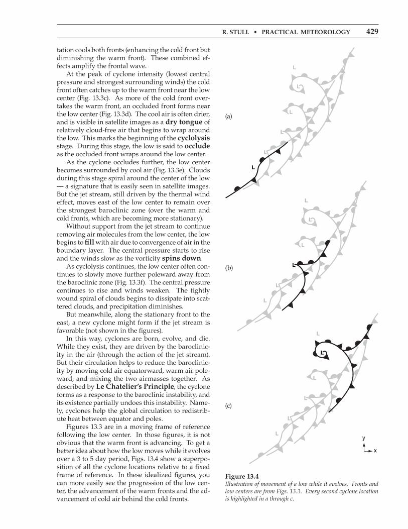
r. stull • practical MEtEorology 429
tation cools both fronts (enhancing the cold front but diminishing the warm front). These combined ef-fects amplify the frontal wave. At the peak of cyclone intensity (lowest central pressure and strongest surrounding winds) the cold front often catches up to the warm front near the low center (Fig. 13.3c). As more of the cold front over-takes the warm front, an occluded front forms near the low center (Fig. 13.3d). The cool air is often drier, and is visible in satellite images as a dry tongue of relatively cloud-free air that begins to wrap around the low. This marks the beginning of the cyclolysis stage. During this stage, the low is said to occlude as the occluded front wraps around the low center. As the cyclone occludes further, the low center becomes surrounded by cool air (Fig. 13.3e). Clouds during this stage spiral around the center of the low — a signature that is easily seen in satellite images. But the jet stream, still driven by the thermal wind effect, moves east of the low center to remain over the strongest baroclinic zone (over the warm and cold fronts, which are becoming more stationary). Without support from the jet stream to continue removing air molecules from the low center, the low begins to fill with air due to convergence of air in the boundary layer. The central pressure starts to rise and the winds slow as the vorticity spins down. As cyclolysis continues, the low center often con-tinues to slowly move further poleward away from the baroclinic zone (Fig. 13.3f). The central pressure continues to rise and winds weaken. The tightly wound spiral of clouds begins to dissipate into scat-tered clouds, and precipitation diminishes. But meanwhile, along the stationary front to the east, a new cyclone might form if the jet stream is favorable (not shown in the figures). In this way, cyclones are born, evolve, and die. While they exist, they are driven by the baroclinic-ity in the air (through the action of the jet stream). But their circulation helps to reduce the baroclinic-ity by moving cold air equatorward, warm air pole-ward, and mixing the two airmasses together. As described by le chatelier’s principle, the cyclone forms as a response to the baroclinic instability, and its existence partially undoes this instability. Name-ly, cyclones help the global circulation to redistrib-ute heat between equator and poles. Figures 13.3 are in a moving frame of reference following the low center. In those figures, it is not obvious that the warm front is advancing. To get a better idea about how the low moves while it evolves over a 3 to 5 day period, Figs. 13.4 show a superpo-sition of all the cyclone locations relative to a fixed frame of reference. In these idealized figures, you can more easily see the progression of the low cen-ter, the advancement of the warm fronts and the ad-vancement of cold air behind the cold fronts.
Figure 13.4Illustration of movement of a low while it evolves. Fronts and low centers are from Figs. 13.3. Every second cyclone location is highlighted in a through c.
(a)
(b)
(c)
430 chaptEr 13 • Extratropical cyclonEs
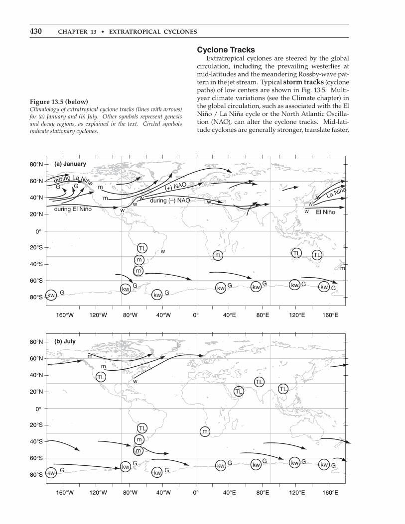
Cyclone tracks Extratropical cyclones are steered by the global circulation, including the prevailing westerlies at mid-latitudes and the meandering Rossby-wave pat-tern in the jet stream. Typical storm tracks (cyclone paths) of low centers are shown in Fig. 13.5. Multi-year climate variations (see the Climate chapter) in the global circulation, such as associated with the El Niño / La Niña cycle or the North Atlantic Oscilla-tion (NAO), can alter the cyclone tracks. Mid-lati-tude cyclones are generally stronger, translate faster,
Figure 13.5 (below)Climatology of extratropical cyclone tracks (lines with arrows) for (a) January and (b) July. Other symbols represent genesis and decay regions, as explained in the text. Circled symbols indicate stationary cyclones.
r. stull • practical MEtEorology 431
and are further equatorward during winter than in summer. One favored cyclogenesis region is just east of large mountain ranges (shown by the “m” sym-bol in Fig. 13.5; see lee cyclogenesis later in this chapter). Other cyclogenesis regions are over warm ocean boundary currents along the western edge of oceans (shown by the symbol “w” in the figure), such as the gulf stream current off the east coast of N. America, and the Kuroshio current off the east coast of Japan. During winter over such cur-rents are strong sensible and latent heat fluxes from the warm ocean into the air, which adds energy to developing cyclones. Also, the strong wintertime contrast between the cold continent and the warm ocean current causes an intense baroclinic zone that drives a strong jet stream above it due to thermal-wind effects. Cyclones are often strengthened in regions un-der the jet stream just east of troughs. In such re-gions, the jet stream steers the low center toward the east and poleward. Hence, cyclone tracks are often toward the northeast in the N. Hemisphere, and to-ward the southeast in the S. Hemisphere. Cyclones in the Northern Hemisphere typically evolve during a 2 to 7 day period, with most lasting 3 - 5 days. They travel at typical speeds of 12 to 15 m s–1 (43 to 54 km h–1), which means they can move about 5000 km during their life. Namely, they can travel the distance of the continental USA from coast to coast or border to border during their lifetime. Since the Pacific is a larger ocean, cyclones that form off of Japan often die in the Gulf of Alaska just west of British Columbia (BC), Canada — a cyclolysis re-gion known as a cyclone graveyard (G). Quasi-stationary lows are indicated with circles in Fig. 13.5. Some of these form over hot continents in summer as a monsoon circulation. These are called thermal lows (TL), as was explained in the Gener-al Circulation chapter in the section on Hydrostatic Thermal Circulations. Others form as quasi-station-ary lee troughs just east of mountain (m) ranges. In the Southern Hemisphere (Fig. 13.5), cyclones are more uniformly distributed in longitude and throughout the year, compared to the N. Hemi-sphere. One reason is the smaller area of continents in Southern-Hemisphere mid-latitudes and subpo-lar regions. Many propagating cyclones form just north of 50°S latitude, and die just south. The region with greatest cyclone activity (cyclogenesis, tracks, cyclolysis) is a band centered near 60°S. These Southern Hemisphere cyclones last an average of 3 to 5 days, and translate with average speeds faster than 10 m s–1 (= 36 km h–1) toward the east-south-east. A band with average translation speeds faster than 15 m s–1 (= 54 km h–1; or > 10°
inFo • north american Geography
To help you interpret the weather maps, the map and tables give state and province names.
Figure b.canadian postal abbreviations for provinces:AB AlbertaBC British ColumbiaMB ManitobaNB New BrunswickNL Newfoundland & LabradorNS Nova Scotia
NT Northwest TerritoriesNU NunavutON OntarioPE Prince Edward Isl.QC QuebecSK SaskatchewanYT Yukon
usa postal abbreviations for states:AK AlaskaAL AlabamaAR ArkansasAZ ArizonaCA CaliforniaCO ColoradoCT Connect- icutDE DelawareFL FloridaGA GeorgiaHI HawaiiIA IowaID IdahoIL IllinoisIN IndianaKS KansasKY KentuckyLA LouisianaMA Massa- chusetts
MD MarylandME MaineMI MichiganMN MinnesotaMO MissouriMS MississippiMT MontanaNC North CarolinaND North DakotaNE NebraskaNH New HampshireNJ New JerseyNM New MexicoNV NevadaNY New YorkOH Ohio
OK OklahomaOR OregonPA Pennsyl- vaniaRI Rhode Isl.SC South CarolinaSD South DakotaTN TennesseeTX TexasUT UtahVA VirginiaVT VermontWA Washing- tonWI WisconsinWV West VirginiaWY WyomingDC Wash. DC
432 chaptEr 13 • Extratropical cyclonEs
longitude day–1) extends from south of southwest-ern Africa eastward to south of western Australia. The average track length is 2100 km. The normal cyclone graveyard (G, cyclolysis region) in the S. Hemisphere is in the circumpolar trough (be-tween 65°S and the Antarctic coastline). Seven stationary centers of enhanced cyclone activity occur around the coast of Antarctica, dur-ing both winter and summer. Some of these are believed to be a result of fast katabatic (cold downslope) winds flowing off the steep Antarctic terrain (see the Fronts & Airmasses chapter). When these very cold winds reach the relatively warm un-frozen ocean, strong heat fluxes from the ocean into the air contribute energy into developing cyclones. Also the downslope winds can be channeled by the terrain to cause cyclonic rotation. But some of the seven stationary centers might not be real — some might be caused by improper reduction of surface pressure to sea-level pressure. These seven centers are labeled with “kw”, indicating a combination of katabatic winds and relatively warm sea surface.
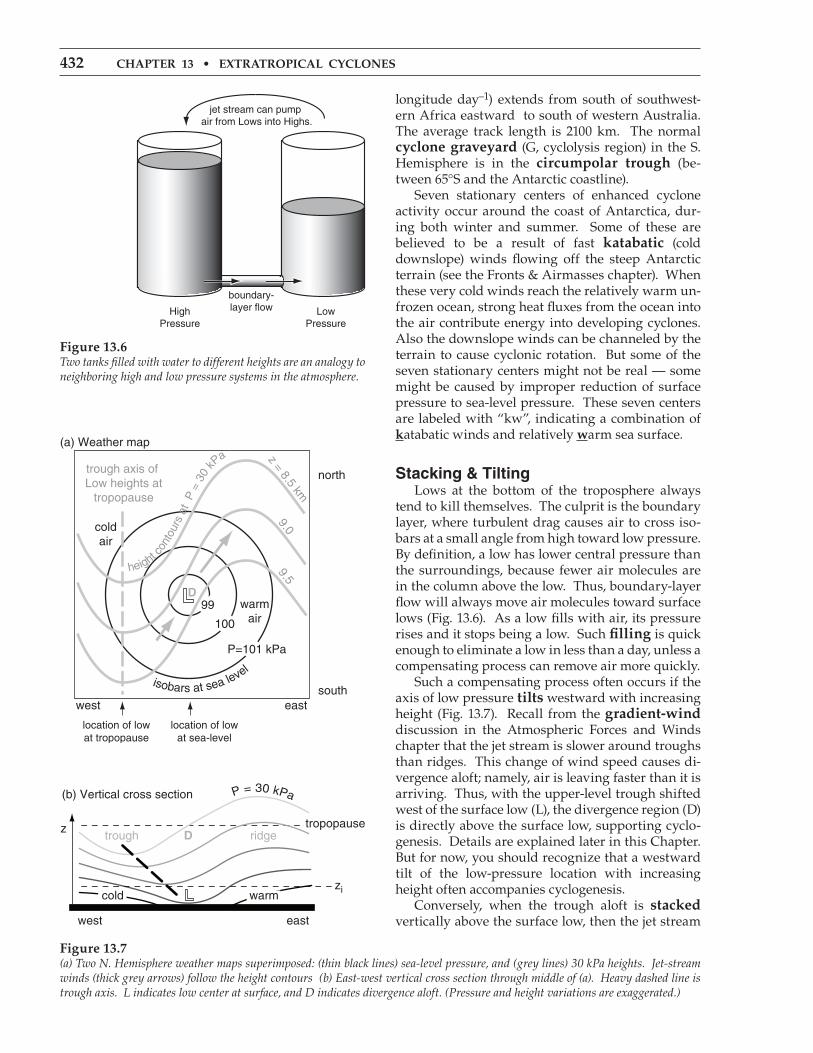
stacking & tilting Lows at the bottom of the troposphere always tend to kill themselves. The culprit is the boundary layer, where turbulent drag causes air to cross iso-bars at a small angle from high toward low pressure. By definition, a low has lower central pressure than the surroundings, because fewer air molecules are in the column above the low. Thus, boundary-layer flow will always move air molecules toward surface lows (Fig. 13.6). As a low fills with air, its pressure rises and it stops being a low. Such filling is quick enough to eliminate a low in less than a day, unless a compensating process can remove air more quickly. Such a compensating process often occurs if the axis of low pressure tilts westward with increasing height (Fig. 13.7). Recall from the gradient-wind discussion in the Atmospheric Forces and Winds chapter that the jet stream is slower around troughs than ridges. This change of wind speed causes di-vergence aloft; namely, air is leaving faster than it is arriving. Thus, with the upper-level trough shifted west of the surface low (L), the divergence region (D) is directly above the surface low, supporting cyclo-genesis. Details are explained later in this Chapter. But for now, you should recognize that a westward tilt of the low-pressure location with increasing height often accompanies cyclogenesis. Conversely, when the trough aloft is stacked vertically above the surface low, then the jet stream
Figure 13.6Two tanks filled with water to different heights are an analogy to neighboring high and low pressure systems in the atmosphere.
Figure 13.7(a) Two N. Hemisphere weather maps superimposed: (thin black lines) sea-level pressure, and (grey lines) 30 kPa heights. Jet-stream winds (thick grey arrows) follow the height contours (b) East-west vertical cross section through middle of (a). Heavy dashed line is trough axis. L indicates low center at surface, and D indicates divergence aloft. (Pressure and height variations are exaggerated.)
r. stull • practical MEtEorology 433
is not pumping air out of the low, and the low fills due to the unrelenting boundary-layer flow. Thus, vertical stacking is associated with cyclolysis.
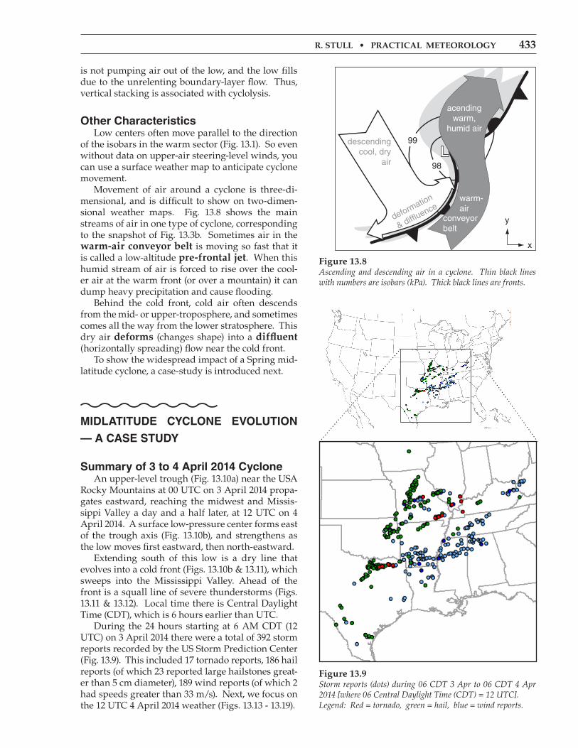
other Characteristics Low centers often move parallel to the direction of the isobars in the warm sector (Fig. 13.1). So even without data on upper-air steering-level winds, you can use a surface weather map to anticipate cyclone movement. Movement of air around a cyclone is three-di-mensional, and is difficult to show on two-dimen-sional weather maps. Fig. 13.8 shows the main streams of air in one type of cyclone, corresponding to the snapshot of Fig. 13.3b. Sometimes air in the warm-air conveyor belt is moving so fast that it is called a low-altitude pre-frontal jet. When this humid stream of air is forced to rise over the cool-er air at the warm front (or over a mountain) it can dump heavy precipitation and cause flooding. Behind the cold front, cold air often descends from the mid- or upper-troposphere, and sometimes comes all the way from the lower stratosphere. This dry air deforms (changes shape) into a diffluent (horizontally spreading) flow near the cold front. To show the widespread impact of a Spring mid-latitude cyclone, a case-study is introduced next.
Midlatitude CyClone evolution
— a Case study
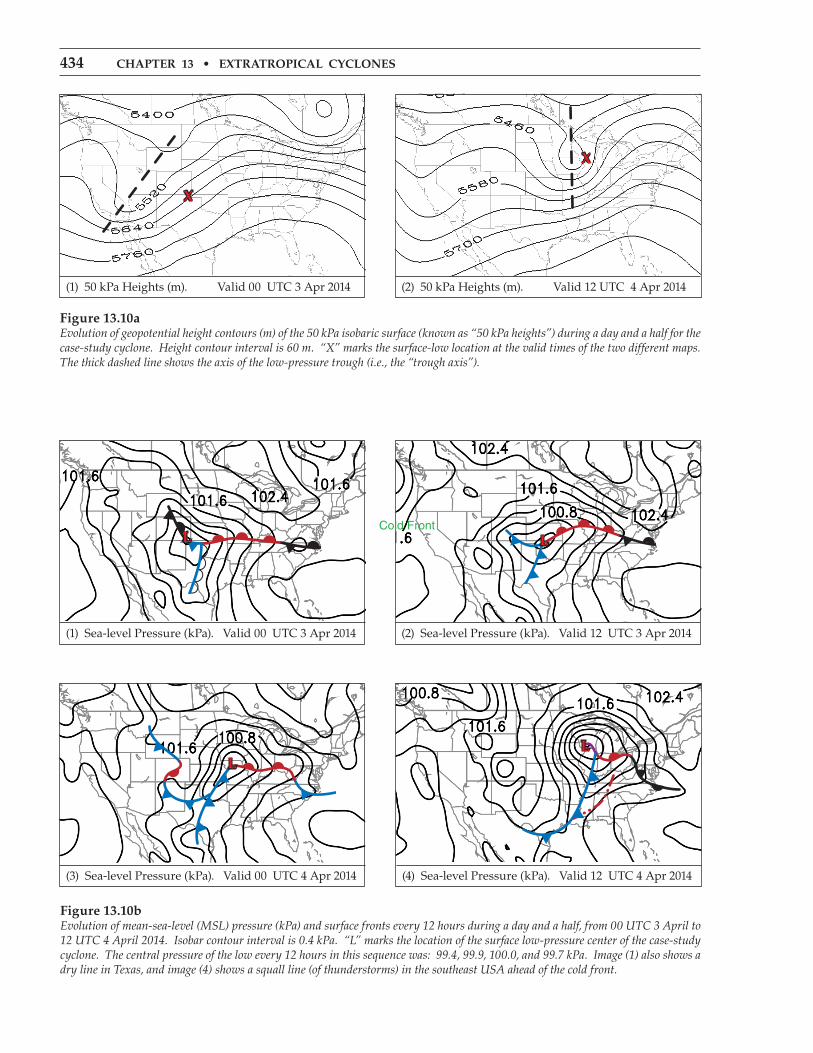
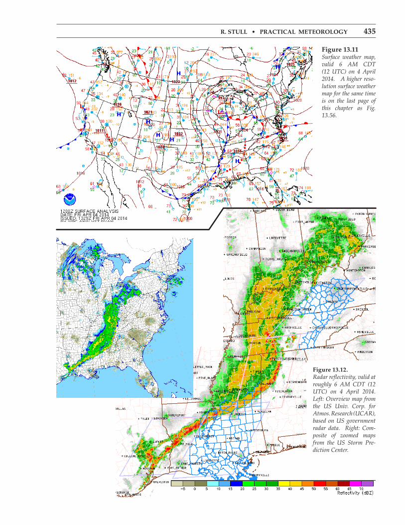
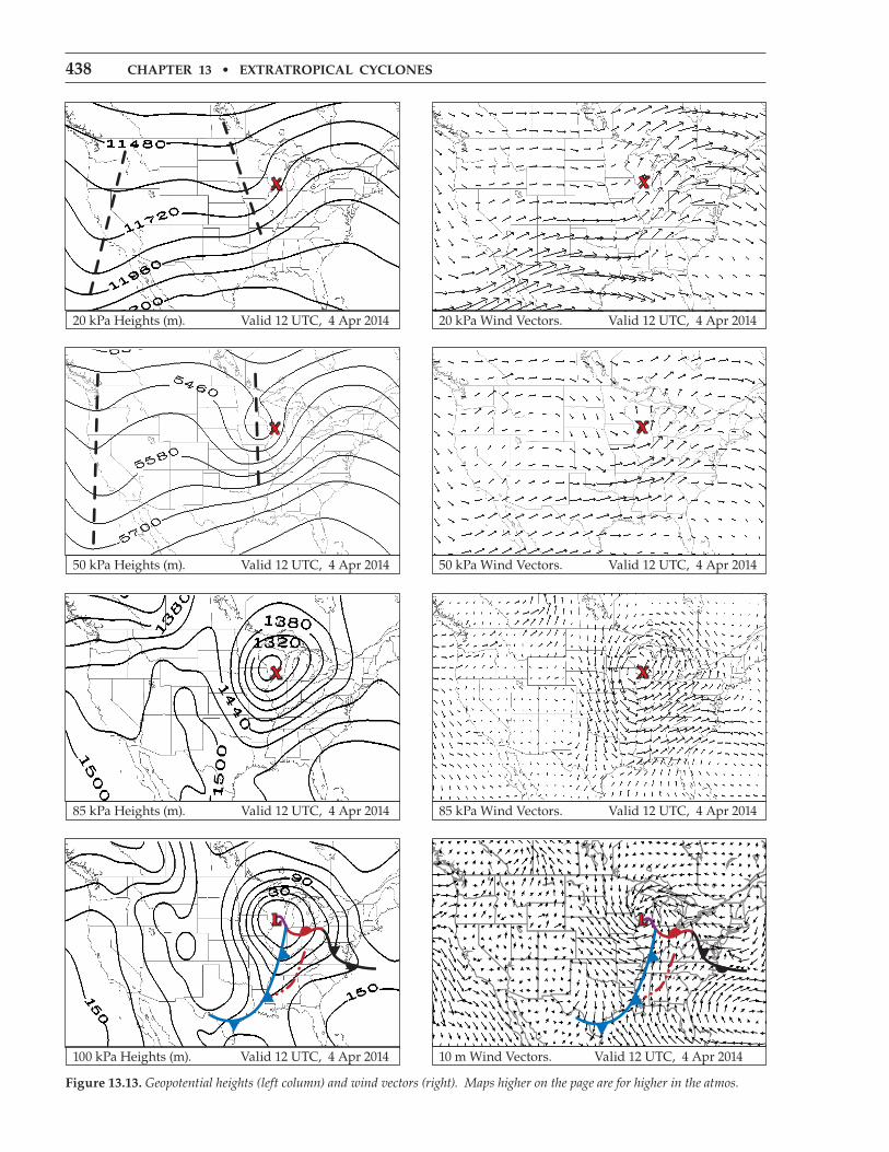
summary of 3 to 4 april 2014 Cyclone An upper-level trough (Fig. 13.10a) near the USA Rocky Mountains at 00 UTC on 3 April 2014 propa-gates eastward, reaching the midwest and Missis-sippi Valley a day and a half later, at 12 UTC on 4 April 2014. A surface low-pressure center forms east of the trough axis (Fig. 13.10b), and strengthens as the low moves first eastward, then north-eastward. Extending south of this low is a dry line that evolves into a cold front (Figs. 13.10b & 13.11), which sweeps into the Mississippi Valley. Ahead of the front is a squall line of severe thunderstorms (Figs. 13.11 & 13.12). Local time there is Central Daylight Time (CDT), which is 6 hours earlier than UTC. During the 24 hours starting at 6 AM CDT (12 UTC) on 3 April 2014 there were a total of 392 storm reports recorded by the US Storm Prediction Center (Fig. 13.9). This included 17 tornado reports, 186 hail reports (of which 23 reported large hailstones great-er than 5 cm diameter), 189 wind reports (of which 2 had speeds greater than 33 m/s). Next, we focus on the 12 UTC 4 April 2014 weather (Figs. 13.13 - 13.19).
Figure 13.8Ascending and descending air in a cyclone. Thin black lines with numbers are isobars (kPa). Thick black lines are fronts.
Figure 13.9Storm reports (dots) during 06 CDT 3 Apr to 06 CDT 4 Apr 2014 [where 06 Central Daylight Time (CDT) = 12 UTC]. Legend: Red = tornado, green = hail, blue = wind reports.
434 chaptEr 13 • Extratropical cyclonEs
Figure 13.10aEvolution of geopotential height contours (m) of the 50 kPa isobaric surface (known as “50 kPa heights”) during a day and a half for the case-study cyclone. Height contour interval is 60 m. “X” marks the surface-low location at the valid times of the two different maps. The thick dashed line shows the axis of the low-pressure trough (i.e., the “trough axis”).
Figure 13.10bEvolution of mean-sea-level (MSL) pressure (kPa) and surface fronts every 12 hours during a day and a half, from 00 UTC 3 April to 12 UTC 4 April 2014. Isobar contour interval is 0.4 kPa. “L” marks the location of the surface low-pressure center of the case-study cyclone. The central pressure of the low every 12 hours in this sequence was: 99.4, 99.9, 100.0, and 99.7 kPa. Image (1) also shows a dry line in Texas, and image (4) shows a squall line (of thunderstorms) in the southeast USA ahead of the cold front.
x
(1) 50 kPa Heights (m). Valid 00 UTC 3 Apr 2014
x
(2) 50 kPa Heights (m). Valid 12 UTC 4 Apr 2014
(1) Sea-level Pressure (kPa). Valid 00 UTC 3 Apr 2014
l
(3) Sea-level Pressure (kPa). Valid 00 UTC 4 Apr 2014
l
(2) Sea-level Pressure (kPa). Valid 12 UTC 3 Apr 2014
l
(4) Sea-level Pressure (kPa). Valid 12 UTC 4 Apr 2014
l
r. stull • practical MEtEorology 435
Figure 13.12. Radar reflectivity, valid at roughly 6 AM CDT (12 UTC) on 4 April 2014. Left: Overview map from the US Univ. Corp. for Atmos. Research (UCAR), based on US government radar data. Right: Com-posite of zoomed maps from the US Storm Pre-diction Center.
Figure 13.11Surface weather map, valid 6 AM CDT (12 UTC) on 4 April 2014. A higher reso-lution surface weather map for the same time is on the last page of this chapter as Fig. 13.56.
436 chaptEr 13 • Extratropical cyclonEs
inFo • isosurfaces & their utility
Lows and other synoptic features have five-di-mensions (3-D spatial structure + 1-D time evolution + 1-D multiple variables). To accurately analyze and forecast the weather, you should try to form in your mind a multi-dimensional picture of the weather. Although some computer-graphics packages can display 5-dimensional data, most of the time you are stuck with flat 2-D weather maps or graphs. By viewing multiple 2-D slices of the atmosphere as drawn on weather maps (Fig. c), you can picture the 5-D structure. Examples of such 2-D maps include: • uniform height maps• isobaric (uniform pressure) maps• isentropic (uniform potential temperature) maps• thickness maps• vertical cross-section maps• time-height maps• time-variable maps (meteograms)Computer animations of maps can show time evolu-tions. In Chapter 1 is a table of other iso-surfaces.
Figure cA set of weather maps for different altitudes helps you gain a 3-D perspective of the weather. MSL = mean sea level.
height Mean-sea-level (Msl) maps represent a uniform height of z = 0 relative to the ocean surface. For most land areas that are above sea level, these maps are cre-ated by extrapolating atmospheric conditions below ground. (A few land-surface locations are below sea level, such as Death Valley and the Salton Sea USA, or the Dead Sea in Israel and Jordan). Meteorologists commonly plot air pressure (re-duced to sea level) and fronts on this uniform-height surface. These are called “MSL pressure” maps. (continues in next column)
inFo • isosurfaces (continuation)
Pressure Recall that pressure decreases monotonically with increasing altitude. Thus, lower pressures correspond to higher heights. For any one pressure, such as 70 kPa (which is about 3 km above sea level on average), that pressure is closer to the ground (i.e., less than 3 km) in some lo-cations and is further from the ground in other loca-tions, as was discussed in the Forces and Winds chap-ter. If you conceptually draw a surface that passes through all the points that have pressure 70 kPa, then that isobaric surface looks like rolling terrain with peaks, valleys (troughs), and ridges. Like a topographic map, you could draw contour lines connecting points of the same height. This is called a “70 kPa height” chart. Low heights on an isobaric surface correspond to low pressure on a uni-form-height surface. Back to the analogy of hilly terrain, suppose you went hiking with a thermometer and measured the air temperature at eye level at many locations within a hilly region. You could write those temperatures on a map and then draw isotherms connecting points of the same temperature. But you would realize that these temperatures on your map correspond to the hilly terrain that had ridges and valleys. You can do the same with isobaric charts; namely, you can plot the temperatures that are found at dif-ferent locations on the undulating isobaric surface. If you did this for the 70 kPa isobaric surface, you would have a “70 kPa isotherm” chart. You can plot any variable on any isobaric surface, such as “90 kPa isohumes”, “50 kPa vorticity”, “30 kPa isotachs”, etc. You can even plot multiple weather variables on any single isobaric map, such as “30 kPa heights and isotachs” or “50 kPa heights and vorticity” (Fig. c). The first chart tells you information about jet-stream speed and direction, and the second chart can be used to estimate cyclogenesis processes.
thickness Now picture two different isobaric surfaces over the same region, such as sketched a the top of Fig. c. An example is 100 kPa heights and 50 kPa heights. At each location on the map, you could measure the height difference between these two pressure surfac-es, which tells you the thickness of air in that layer. After drawing isopleths connecting points of equal thickness, the resulting contour map is known as a “100 to 50 kPa thickness” map. You learned in the General Circulation chapter that the thermal-wind vectors are parallel to thick-ness contours, and that these vectors indicate shear in the geostrophic wind. That chapter also showed that the 100-50 kPa thickness is proportional to average temperature in the bottom half of the troposphere. (continues on next page)
r. stull • practical MEtEorology 437
inFo • isosurfaces (continued)
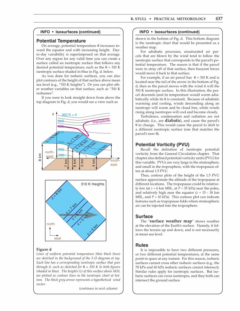
Potential temperature On average, potential temperature θ increases to-ward the equator and with increasing height. Day-to-day variability is superimposed on that average. Over any region for any valid time you can create a surface called an isentropic surface that follows any desired potential temperature, such as the θ = 310 K isentropic surface shaded in blue in Fig. d. below. As was done for isobaric surfaces, you can also plot contours of the height of that surface above mean sea level (e.g., “310 K heights”). Or you can plot oth-er weather variables on that surface, such as “310 K isohumes”. If you were to look straight down from above the top diagram in Fig. d, you would see a view such as
Figure dLines of uniform potential temperature (thin black lines) are sketched in the background of the 3-D diagram at top. Each line has a corresponding isentropic surface that goes through it, such as sketched for θ = 310 K in both figures (shaded in blue). The heights (z) of this surface above MSL are plotted as contour lines in the isentropic chart at bot-tom. The thick grey arrow represents a hypothetical wind vector. (continues in next column)
inFo • isosurfaces (continued)
shown in the bottom of Fig. d. This bottom diagram is the isentropic chart that would be presented as a weather map. For adiabatic processes, unsaturated air par-cels that are blown by the wind tend to follow the isentropic surface that corresponds to the parcel’s po-tential temperature. The reason is that if the parcel were to stray off of that surface, then buoyant forces would move it back to that surface. For example, if an air parcel has θ = 310 K and is located near the tail of the arrow in the bottom of Fig. d, then as the parcel moves with the wind it will the 310 K isentropic surface. In this illustration, the par-cel descends (and its temperature would warm adia-batically while its θ is constant). Because of adiabatic warming and cooling, winds descending along an isentrope will warm and be cloud free, while winds rising along isentropes will cool and become cloudy. Turbulence, condensation and radiation are not adiabatic (i.e., are diabatic), and cause the parcel’s θ to change. This would cause the parcel to shift to a different isentropic surface (one that matches the parcel’s new θ).
Potential vorticity (Pvu) Recall the definition of isentropic potential vorticity from the General Circulation chapter. That chapter also defined potential vorticity units (PVU) for this variable. PVUs are very large in the stratosphere, and small in the troposphere, with the tropopause of-ten at about 1.5 PVU. Thus, contour plots of the height of the 1.5 PVU surface approximate the altitude of the tropopause at different locations. The tropopause could be relative-ly low (at z ≈ 6 km MSL, at P ≈ 35 kPa) near the poles, and relatively high near the equator (z ≈ 15 - 18 km MSL, and P ≈ 10 kPa). This contour plot can indicate features such as tropopause folds where stratospheric air can be injected into the troposphere.
surface The “surface weather map” shows weather at the elevation of the Earth’s surface. Namely, it fol-lows the terrain up and down, and is not necessarily at mean sea level.
rules It is impossible to have two different pressures, or two different potential temperatures, at the same point in space at any instant. For this reason, isobaric surfaces cannot cross other isobaric surfaces (e.g., the 70 kPa and 60 kPa isobaric surfaces cannot intersect). Similar rules apply for isentropic surfaces. But iso-baric surfaces can cross isentropes, and they both can intersect the ground surface.
438 chaptEr 13 • Extratropical cyclonEs
50 kPa Wind Vectors. Valid 12 UTC, 4 Apr 2014
x
20 kPa Wind Vectors. Valid 12 UTC, 4 Apr 2014
x
85 kPa Wind Vectors. Valid 12 UTC, 4 Apr 2014
x
85 kPa Heights (m). Valid 12 UTC, 4 Apr 2014
x
Figure 13.13. Geopotential heights (left column) and wind vectors (right). Maps higher on the page are for higher in the atmos.
100 kPa Heights (m). Valid 12 UTC, 4 Apr 2014
l
10 m Wind Vectors. Valid 12 UTC, 4 Apr 2014
l
20 kPa Heights (m). Valid 12 UTC, 4 Apr 2014
x
x
50 kPa Heights (m). Valid 12 UTC, 4 Apr 2014
r. stull • practical MEtEorology 439
20 kPa Isotachs (m s–1). Valid 12 UTC, 4 Apr 2014
x
50 kPa Temperature (°C). Valid 12 UTC, 4 Apr 2014
x
20 kPa Temperature (°C). Valid 12 UTC, 4 Apr 2014
x
85 kPa Temperature (°C). Valid 12 UTC, 4 Apr 2014
x
50 kPa Abs.Vorticity (10–5 s–1). Valid 12 UTC, 4 Apr 2014
x
85 kPa Abs. Vorticity (10–5 s–1). Valid 12 UTC, 4 Apr 2014
x
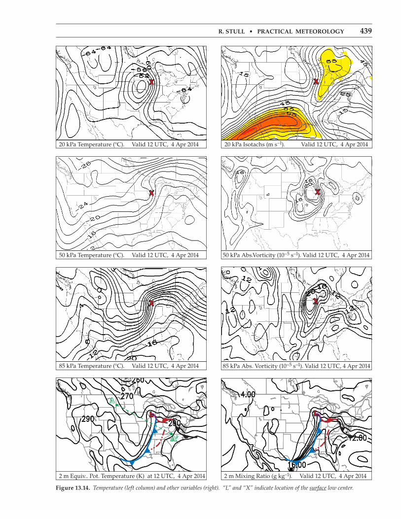
Figure 13.14. Temperature (left column) and other variables (right). “L” and “X” indicate location of the surface low center.
2 m Mixing Ratio (g kg–1). Valid 12 UTC, 4 Apr 2014
l
2 m Equiv.. Pot. Temperature (K) at 12 UTC, 4 Apr 2014
l
a
a’
440 chaptEr 13 • Extratropical cyclonEs
20 kPa Streamlines. Valid 12 UTC, 4 Apr 2014
x
Precipitable water (mm). Valid 12 UTC, 4 Apr 2014
l
x
20 kPa Divergence (10–5 s–1). Valid 12 UTC, 4 Apr 2014
70 kPa Temperature (°C). Valid 12 UTC, 4 Apr 2014
x
MSL P (kPa), 85 kPa T (°C) & 1 h Precip.(in) at 13 UTC, 4 Apr 2014
l
70 kPa Heights (m). Valid 12 UTC, 4 Apr 2014
x
100 - 50 kPa Thickness. Valid 12 UTC, 4 Apr 2014
x
Figure 13.15. Maps higher on the page are for higher in the atmosphere. “L” and “X” indicate location of surface low-pressure cen-ter.
Figure 13.16. Thickness (m) between the 100 kPa and 50 kPa isobaric surfaces.
r. stull • practical MEtEorology 441
x
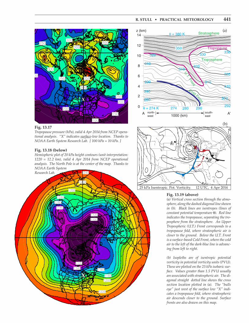
Fig. 13.17Tropopause pressure (hPa), valid 4 Apr 2014 from NCEP opera-tional analysis. “X” indicates surface-low location. Thanks to NOAA Earth System Research Lab. [ 100 hPa = 10 kPa. ]
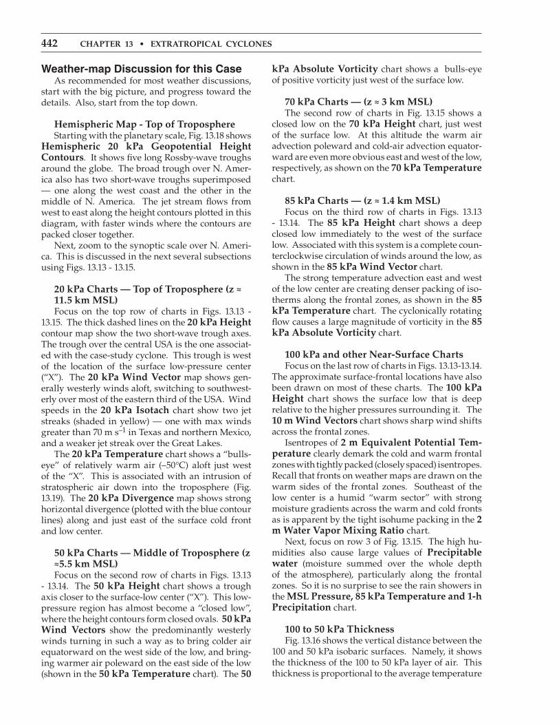
Fig. 13.18 (below)Hemispheric plot of 20 kPa height contours (unit interpretation: 1220 = 12.2 km), valid 4 Apr 2014 from NCEP operational analysis. The North Pole is at the center of the map. Thanks to NOAA Earth System Research Lab.
x
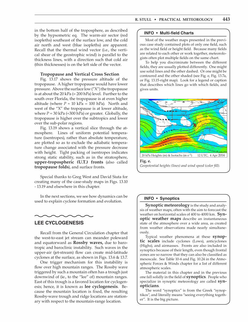
Fig. 13.19 (above)(a) Vertical cross section through the atmo-sphere, along the dashed diagonal line shown in (b). Black lines are isentropes (lines of constant potential temperature θ). Red line indicates the tropopause, separating the tro-posphere from the stratosphere. An Upper Tropospheric (U.T.) Front corresponds to a tropopause fold, where stratospheric air is closer to the ground. Below the U.T. Front is a surface-based Cold Front, where the cold air to the left of the dark-blue line is advanc-ing from left to right.
(b) Isopleths are of isentropic potential vorticity in potential vorticity units (PVU). These are plotted on the 25 kPa isobaric sur-face. Values greater than 1.5 PVU usually are associated with stratospheric air. The di-agonal straight dotted line shows the cross section location plotted in (a). The “bulls eye” just west of the surface low “X” indi-cates a tropopause fold, where stratospheric air descends closer to the ground. Surface fronts are also drawn on this map.
(a)
25 kPa Isentropic. Pot. Vorticity. 12 UTC, 4 Apr 2014
(b)
a
a’
x
442 chaptEr 13 • Extratropical cyclonEs
kpa absolute Vorticity chart shows a bulls-eye of positive vorticity just west of the surface low.
70 kpa charts — (z ≈ 3 km Msl) The second row of charts in Fig. 13.15 shows a closed low on the 70 kpa height chart, just west of the surface low. At this altitude the warm air advection poleward and cold-air advection equator-ward are even more obvious east and west of the low, respectively, as shown on the 70 kpa temperature chart.
85 kpa charts — (z ≈ 1.4 km Msl) Focus on the third row of charts in Figs. 13.13 - 13.14. The 85 kpa height chart shows a deep closed low immediately to the west of the surface low. Associated with this system is a complete coun-terclockwise circulation of winds around the low, as shown in the 85 kpa Wind Vector chart. The strong temperature advection east and west of the low center are creating denser packing of iso-therms along the frontal zones, as shown in the 85 kpa temperature chart. The cyclonically rotating flow causes a large magnitude of vorticity in the 85 kpa absolute Vorticity chart.
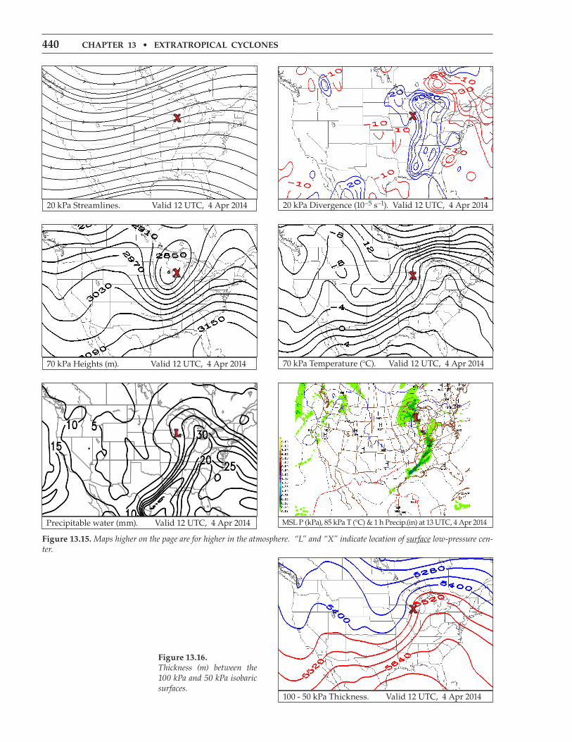
100 kpa and other near-surface charts Focus on the last row of charts in Figs. 13.13-13.14. The approximate surface-frontal locations have also been drawn on most of these charts. The 100 kpa height chart shows the surface low that is deep relative to the higher pressures surrounding it. The 10 m Wind Vectors chart shows sharp wind shifts across the frontal zones. Isentropes of 2 m Equivalent potential tem-perature clearly demark the cold and warm frontal zones with tightly packed (closely spaced) isentropes. Recall that fronts on weather maps are drawn on the warm sides of the frontal zones. Southeast of the low center is a humid “warm sector” with strong moisture gradients across the warm and cold fronts as is apparent by the tight isohume packing in the 2 m Water Vapor Mixing ratio chart. Next, focus on row 3 of Fig. 13.15. The high hu-midities also cause large values of precipitable water (moisture summed over the whole depth of the atmosphere), particularly along the frontal zones. So it is no surprise to see the rain showers in the Msl pressure, 85 kpa temperature and 1-h precipitation chart.
100 to 50 kpa thickness Fig. 13.16 shows the vertical distance between the 100 and 50 kPa isobaric surfaces. Namely, it shows the thickness of the 100 to 50 kPa layer of air. This thickness is proportional to the average temperature
Weather-map discussion for this Case As recommended for most weather discussions, start with the big picture, and progress toward the details. Also, start from the top down.
hemispheric Map - top of troposphere Starting with the planetary scale, Fig. 13.18 shows hemispheric 20 kpa geopotential height contours. It shows five long Rossby-wave troughs around the globe. The broad trough over N. Amer-ica also has two short-wave troughs superimposed — one along the west coast and the other in the middle of N. America. The jet stream flows from west to east along the height contours plotted in this diagram, with faster winds where the contours are packed closer together. Next, zoom to the synoptic scale over N. Ameri-ca. This is discussed in the next several subsections using Figs. 13.13 - 13.15.
20 kpa charts — top of troposphere (z ≈ 11.5 km Msl)
Focus on the top row of charts in Figs. 13.13 - 13.15. The thick dashed lines on the 20 kpa height contour map show the two short-wave trough axes. The trough over the central USA is the one associat-ed with the case-study cyclone. This trough is west of the location of the surface low-pressure center (“X”). The 20 kpa Wind Vector map shows gen-erally westerly winds aloft, switching to southwest-erly over most of the eastern third of the USA. Wind speeds in the 20 kpa isotach chart show two jet streaks (shaded in yellow) — one with max winds greater than 70 m s–1 in Texas and northern Mexico, and a weaker jet streak over the Great Lakes. The 20 kpa temperature chart shows a “bulls-eye” of relatively warm air (–50°C) aloft just west of the “X”. This is associated with an intrusion of stratospheric air down into the troposphere (Fig. 13.19). The 20 kpa Divergence map shows strong horizontal divergence (plotted with the blue contour lines) along and just east of the surface cold front and low center.
50 kpa charts — Middle of troposphere (z ≈5.5 km Msl)
Focus on the second row of charts in Figs. 13.13 - 13.14. The 50 kpa height chart shows a trough axis closer to the surface-low center (“X”). This low-pressure region has almost become a “closed low”, where the height contours form closed ovals. 50 kpa Wind Vectors show the predominantly westerly winds turning in such a way as to bring colder air equatorward on the west side of the low, and bring-ing warmer air poleward on the east side of the low (shown in the 50 kpa temperature chart). The 50
r. stull • practical MEtEorology 443
in the bottom half of the troposphere, as described by the hypsometric eq. The warm-air sector (red isopleths) southeast of the surface low, and the cold air north and west (blue isopleths) are apparent. Recall that the thermal wind vector (i.e., the verti-cal shear of the geostrophic wind) is parallel to the thickness lines, with a direction such that cold air (thin thicknesses) is on the left side of the vector.
tropopause and Vertical cross section Fig. 13.17 shows the pressure altitude of the tropopause. A higher tropopause would have lower pressure. Above the surface low (”X”) the tropopause is at about the 20 kPa (= 200 hPa) level. Further to the south over Florida, the tropopause is at even higher altitude (where P ≈ 10 kPa = 100 hPa). North and west of the “X” the tropopause is at lower altitude, where P = 30 kPa (=300 hPa) or greater. Globally, the tropopause is higher over the subtropics and lower over the sub-polar regions. Fig. 13.19 shows a vertical slice through the at-mosphere. Lines of uniform potential tempera-ture (isentropes), rather than absolute temperature, are plotted so as to exclude the adiabatic tempera-ture change associated with the pressure decrease with height. Tight packing of isentropes indicates strong static stability, such as in the stratosphere, upper-tropospheric (u.t.) fronts (also called tropopause folds), and surface fronts.
Special thanks to Greg West and David Siuta for creating many of the case-study maps in Figs. 13.10 - 13.19 and elsewhere in this chapter.
In the next sections, we see how dynamics can be used to explain cyclone formation and evolution.
lee CyCloGenesis
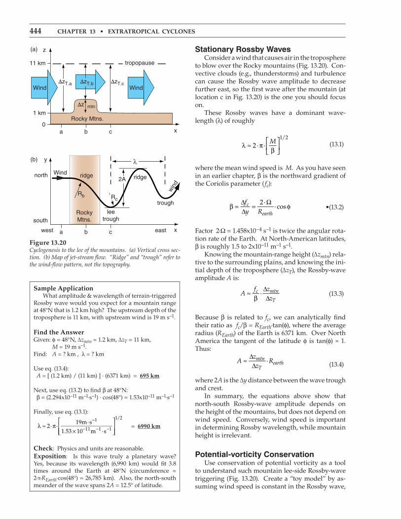
Recall from the General Circulation chapter that the west-to-east jet stream can meander poleward and equatorward as rossby waves, due to baro-tropic and baroclinic instability. Such waves in the upper-air (jet-stream) flow can create mid-latitude cyclones at the surface, as shown in Figs. 13.6 & 13.7. One trigger mechanism for this instability is flow over high mountain ranges. The Rossby wave triggered by such a mountain often has a trough just downwind of (ie., to the “lee” of) mountain ranges. East of this trough is a favored location for cyclogen-esis; hence, it is known as lee cyclogenesis. Be-cause the mountain location is fixed, the resulting Rossby-wave trough and ridge locations are station-ary with respect to the mountain-range location.
inFo • Multi-field Charts
Most of the weather maps presented in the previ-ous case study contained plots of only one field, such as the wind field or height field. Because many fields are related to each other or work together, meteorolo-gists often plot multiple fields on the same chart. To help you discriminate between the different fields, they are usually plotted differently. One might use solid lines and the other dashed. Or one might be contoured and the other shaded (see Fig. e, Fig. 13.7a, or Fig. 13.15-right map). Look for a legend or caption that describes which lines go with which fields, and gives units.
20 kPa Heights (m) & Isotachs (m s–1) 12 UTC, 4 Apr 2014
x
Fig. e.Geopotential heights (lines) and wind speed (color fill).
inFo • synoptics
synoptic meteorology is the study and analy-sis of weather maps, often with the aim to forecast the weather on horizontal scales of 400 to 4000 km. syn-optic weather maps describe an instantaneous state of the atmosphere over a wide area, as created from weather observations made nearly simultane-ously. Typical weather phenomena at these synop-tic scales include cyclones (Lows), anticyclones (Highs), and airmasses. Fronts are also included in synoptics because of their length, even though frontal zones are so narrow that they can also be classified as mesoscale. See Table 10-6 and Fig. 10.24 in the Atmo-spheric Forces & Winds chapter for a list of different atmospheric scales. The material in this chapter and in the previous one fall solidly in the field of synoptics. People who specialize in synoptic meteorology are called syn-opticians. The word “synoptics” is from the Greek “synop-tikos”, and literally means “seeing everything togeth-er”. It is the big picture.
444 chaptEr 13 • Extratropical cyclonEs
stationary rossby Waves Consider a wind that causes air in the troposphere to blow over the Rocky mountains (Fig. 13.20). Con-vective clouds (e.g., thunderstorms) and turbulence can cause the Rossby wave amplitude to decrease further east, so the first wave after the mountain (at location c in Fig. 13.20) is the one you should focus on. These Rossby waves have a dominant wave-length (λ) of roughly
λβ
≈ π
2
1 2
· ·/
M (13.1)
where the mean wind speed is M. As you have seen in an earlier chapter, β is the northward gradient of the Coriolis parameter ( fc):
β φ=∆∆
=fy Rc
earth
2 ·· cos
Ω •(13.2)
Factor 2·Ω = 1.458x10⁻⁴ s–1 is twice the angular rota-tion rate of the Earth. At North-American latitudes, β is roughly 1.5 to 2x10–11 m–1 s–1. Knowing the mountain-range height (∆zmtn) rela-tive to the surrounding plains, and knowing the ini-tial depth of the troposphere (∆zT), the Rossby-wave amplitude A is:
Af z
zc mtn
T≈
∆∆β
· (13.3)
Because β is related to fc, we can analytically find their ratio as fc/β = REarth·tan(ϕ), where the average radius (REarth) of the Earth is 6371 km. Over North America the tangent of the latitude ϕ is tan(ϕ) ≈ 1. Thus:
Azz
Rmtn
Tearth≈
∆∆
· (13.4)
where 2A is the ∆y distance between the wave trough and crest. In summary, the equations above show that north-south Rossby-wave amplitude depends on the height of the mountains, but does not depend on wind speed. Conversely, wind speed is important in determining Rossby wavelength, while mountain height is irrelevant.
Potential-vorticity Conservation Use conservation of potential vorticity as a tool to understand such mountain lee-side Rossby-wave triggering (Fig. 13.20). Create a “toy model” by as-suming wind speed is constant in the Rossby wave,
sample application What amplitude & wavelength of terrain-triggered Rossby wave would you expect for a mountain range at 48°N that is 1.2 km high? The upstream depth of the troposphere is 11 km, with upstream wind is 19 m s–1.
Find the answerGiven: ϕ = 48°N, ∆zmtn = 1.2 km, ∆zT = 11 km, M = 19 m s–1.Find: A = ? km , λ = ? km
Use eq. (13.4): A = [ (1.2 km) / (11 km) ] · (6371 km) = 695 km
Next, use eq. (13.2) to find β at 48°N: β = (2.294x10⁻¹¹ m–1·s–1) · cos(48°) = 1.53x10⁻¹¹ m–1·s–1
Finally, use eq. (13.1):
λ ≈ π×
−
− − −219
1 53 10 11
1 2
· ··
. ·
/m s
m s
1
1 1 = 6990 km
check: Physics and units are reasonable.Exposition: Is this wave truly a planetary wave? Yes, because its wavelength (6,990 km) would fit 3.8 times around the Earth at 48°N (circumference = 2·π·REarth·cos(48°) = 26,785 km). Also, the north-south meander of the wave spans 2A = 12.5° of latitude.
Figure 13.20Cyclogenesis to the lee of the mountains. (a) Vertical cross sec-tion. (b) Map of jet-stream flow. “Ridge” and “trough” refer to the wind-flow pattern, not the topography.
r. stull • practical MEtEorology 445
and that there is no wind shear affecting vorticity. For this situation, the conservation of potential vorticity ζp is given by eq. (11.25) as:
ζpcM R f
z=
+∆
=( / )
constant •(13.5)
For this toy model, consider the initial winds to be blowing straight toward the Rocky Mountains from the west. These initial winds have no curvature at location “a”, thus R = ∞ and eq. (13.5) becomes:
ζpc a
T a
fz
=∆
.
.
(13.6)
where ∆zT.a is the average depth of troposphere at point “a”. Because potential vorticity is conserved, we can use this fixed value of ζp to see how the Ross-by wave is generated. Let ∆zmtn be the relative mountain height above the surrounding land (Fig. 13.20a). As the air blows over the mountain range, the troposphere becomes thinner as it is squeezed between mountain top and the tropopause at location “b”: ∆zT.b = ∆zT.a – ∆zmtn. But the latitude of the air hasn’t changed much yet, so fc.b ≈ fc.a. Because ∆z has changed, we can solve eq. (13.5) for the radius of curvature needed to main-tain ζp.b = ζp.a.
RM
f z zbc a mtn T a
= −∆ ∆. .·( / ) (13.7)
Namely, in eq. (13.5), when ∆z became smaller while fc was constant, M/R had to also become smaller to keep the ratio constant. But since M/R was initially zero, the new M/R had to become negative. Nega-tive R means anticyclonic curvature. As sketched in Fig. 13.20, such curvature turns the wind toward the equator. But equatorward-moving air experiences smaller Coriolis parameter, requiring that Rb become larger (less curved) to con-serve ζp . Near the east side of the Rocky Mountains the terrain elevation decreases at point “c”, allowing the air thickness ∆z to increase back to is original value. But now the air is closer to the equator where Coriolis parameter is smaller, so the radius of cur-vature Rc at location “c” becomes positive in order to keep potential vorticity constant. This positive vorticity gives that cyclonic curvature that defines the lee trough of the Rossby wave. As was sketched in Fig. 13.7, surface cyclogenesis could be supported just east of the lee trough.
sample application Picture a scenario as plotted in Fig. 13.20, with 25 m s–1 wind at location “a”, mountain height of 1.2 km, tro-posphere thickness of 11 km, and latitude 45°N. What is the value of the initial potential vorticity, and what is the radius of curvature at point “b”?
Find the answerGiven: M = 25 m s–1, ∆zmtn = 1.2 km, Rinitial = ∞, ∆zT = 11 km, ϕ = 45°N. Find: ζp.a = ? m–1·s–1, Rb = ? km
Assumption: Neglect wind shear in the vorticity cal-culation.
Eq. (10.16) can be applied to get the Coriolis parameter fc = (1.458x10⁻⁴ s–1)·sin(45°) = 1.031x10⁻⁴ s–1
Use eq. (13.6):
ζp = × − −1 031 1011
4. skm
1 = 9.37x10⁻⁹ m–1 s–1
Next, apply eq. (13.7) to get the radius of curvature:
Rb =−
× − −( )
( . )·( . / )
25
1 031 10 1 2 114m/s
s km km1 = –2223. km
check: Physics and units are reasonable.Exposition: The negative sign for the radius of cur-vature means that the turn is anticyclonic (clockwise in the N. Hemisphere). Typically, the cyclonic trough curvature is the same order of magnitude as the anti-cyclonic ridge curvature. East of the first trough and west of the next ridge is where cyclogenesis is sup-ported.
446 chaptEr 13 • Extratropical cyclonEs
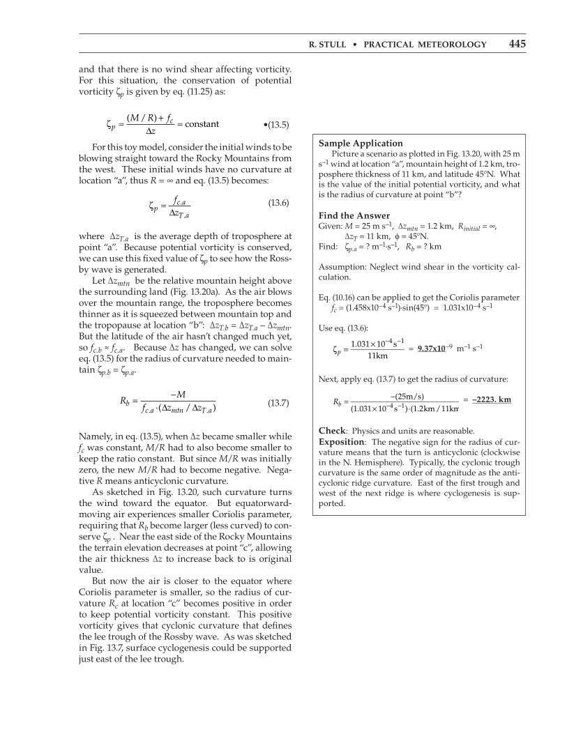
lee-side translation equatorward Suppose an extratropical cyclone (low center) is positioned over the east side of a mountain range in the Northern Hemisphere, as sketched in Fig. 13.21. In this diagram, the green circle and the air above it are the cyclone. Air within this cyclone has posi-tive (cyclonic) vorticity, as represented by the rotat-ing blue air columns in the figure. The locations of these air columns are also moving counterclockwise around the common low center (L) — driven by the synoptic-scale circulation around the low. As column “a” moves to position “b” and then “c”, its vertical extent ∆z stretches. This assumes that the top of the air columns is at the tropopause, while the bottom follows the sloping terrain. Due to conservation of potential vorticity ζp, this stretch-ing must be accompanied by an increase in relative vorticity ∆ζ r : ∆ =ζ α ζr pR2 · · · (13.8)
R is cyclone radius and α = ∆z/∆x is terrain slope. Conversely, as column “c” moves to position “d” and then “a”, its vertical extent shrinks, forcing its relative vorticity to decrease to maintain constant potential vorticity. Hence, the center of action of the low center shifts (translates) equatorward (white ar-row in Fig. 13.21) along the lee side of the mountains, following the region of increasing ζ r . A similar conclusion can be reached by consid-ering conservation of isentropic potential vorticity (IPV). Air in the bottom of column “a” descends and warms adiabatically en route to position “c”, while there is no descent warming at the column top. Hence, the static stability of the column decreases at its equatorward side. This drives an increase in relative vorticity on the equatorward flank of the cyclone to conserve IPV. Again, the cyclone moves equatorward toward the region of greater relative vorticity.
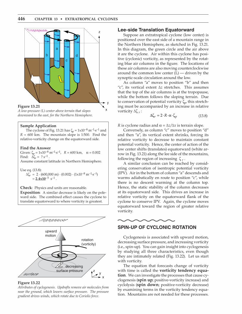
sPin-uP oF CyCloniC rotation
Cyclogenesis is associated with upward motion, decreasing surface pressure, and increasing vorticity (i.e., spin-up). You can gain insight into cyclogenesis by studying all three characteristics, even though they are intimately related (Fig. 13.22). Let us start with vorticity. The equation that forecasts change of vorticity with time is called the vorticity tendency equa-tion. We can investigate the processes that cause cy-clogenesis (spin up; positive-vorticity increase) and cyclolysis (spin down; positive-vorticity decrease) by examining terms in the vorticity tendency equa-tion. Mountains are not needed for these processes.
sample application The cyclone of Fig. 13.21 has ζp = 1x10⁻⁸ m–1·s–1 and R = 600 km. The mountain slope is 1:500. Find the relative-vorticity change on the equatorward side.
Find the answerGiven: ζp = 1x10⁻⁸ m–1·s–1, R = 600 km, α = 0.002Find: ∆ζr = ? s–1 .Assume constant latitude in Northern Hemisphere.
Use eq. (13.8): ∆ζr = 2 · (600,000 m) · (0.002) · (1x10–8 m–1·s–1) = 2.4x10⁻⁵ s–1 .
check: Physics and units are reasonable.Exposition: A similar decrease is likely on the pole-ward side. The combined effect causes the cyclone to translate equatorward to where vorticity is greatest.
Figure 13.22Attributes of cyclogenesis. Updrafts remove air molecules from near the ground, which lowers surface pressure. The pressure gradient drives winds, which rotate due to Coriolis force.
Figure 13.21A low-pressure (L) center above terrain that slopesdownward to the east, for the Northern Hemisphere.
r. stull • practical MEtEorology 447
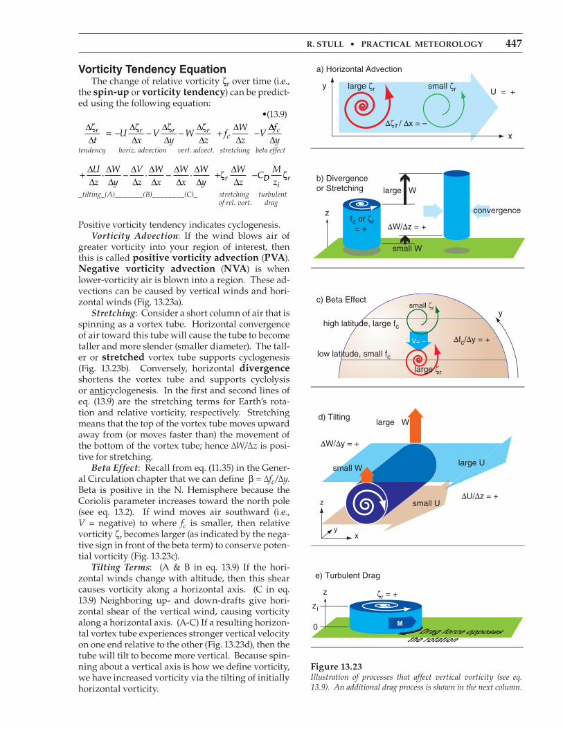
vorticity tendency equation The change of relative vorticity ζr over time (i.e., the spin-up or vorticity tendency) can be predict-ed using the following equation: •(13.9)
∆∆
= − ∆∆
− ∆∆
− ∆∆
+ ∆∆
−ζ ζ ζ ζr r r rct
Ux
Vy
Wz
fWz
V ∆∆∆fyc
tendency horiz. advection vert. advect. stretching beta effect
+ ∆∆
∆∆
− ∆∆
∆∆
− ∆∆
∆∆
+ ∆∆
−Uz
Wy
Vz
Wx
Wx
Wy
Wz
Cr· · · ζ DDi
rMzζ
_tilting_(A)_______(B)________(C)_ stretching turbulent of rel. vort. drag
Positive vorticity tendency indicates cyclogenesis. Vorticity Advection: If the wind blows air of greater vorticity into your region of interest, then this is called positive vorticity advection (pVa). negative vorticity advection (nVa) is when lower-vorticity air is blown into a region. These ad-vections can be caused by vertical winds and hori-zontal winds (Fig. 13.23a). Stretching: Consider a short column of air that is spinning as a vortex tube. Horizontal convergence of air toward this tube will cause the tube to become taller and more slender (smaller diameter). The tall-er or stretched vortex tube supports cyclogenesis (Fig. 13.23b). Conversely, horizontal divergence shortens the vortex tube and supports cyclolysis or anticyclogenesis. In the first and second lines of eq. (13.9) are the stretching terms for Earth’s rota-tion and relative vorticity, respectively. Stretching means that the top of the vortex tube moves upward away from (or moves faster than) the movement of the bottom of the vortex tube; hence ∆W/∆z is posi-tive for stretching. Beta Effect: Recall from eq. (11.35) in the Gener-al Circulation chapter that we can define β = ∆fc/∆y. Beta is positive in the N. Hemisphere because the Coriolis parameter increases toward the north pole (see eq. 13.2). If wind moves air southward (i.e., V = negative) to where fc is smaller, then relative vorticity ζr becomes larger (as indicated by the nega-tive sign in front of the beta term) to conserve poten-tial vorticity (Fig. 13.23c). Tilting Terms: (A & B in eq. 13.9) If the hori-zontal winds change with altitude, then this shear causes vorticity along a horizontal axis. (C in eq. 13.9) Neighboring up- and down-drafts give hori-zontal shear of the vertical wind, causing vorticity along a horizontal axis. (A-C) If a resulting horizon-tal vortex tube experiences stronger vertical velocity on one end relative to the other (Fig. 13.23d), then the tube will tilt to become more vertical. Because spin-ning about a vertical axis is how we define vorticity, we have increased vorticity via the tilting of initially horizontal vorticity.
Figure 13.23Illustration of processes that affect vertical vorticity (see eq. 13.9). An additional drag process is shown in the next column.
448 chaptEr 13 • Extratropical cyclonEs
Turbulence in the atmospheric boundary lay-er (ABL) communicates frictional forces from the ground to the whole ABL. This turbulent drag acts to slow the wind and decrease rotation rates (Fig. 13.23e). Such spin down can cause cyclolysis. However, for cold fronts drag can increase vorticity. As the cold air advances (black arrow in Fig. 13.23f), Coriolis force will turn the winds and create a geostrophic wind Vg (large white arrow). Closer to the leading edge of the front where the cold air is shallower, the winds M subgeostrophic because of the greater drag. The result is a change of wind speed M with distance x that causes positive vorticity. All of the terms in the vorticity-tendency equa-tion must be summed to determine net spin down or spin up.
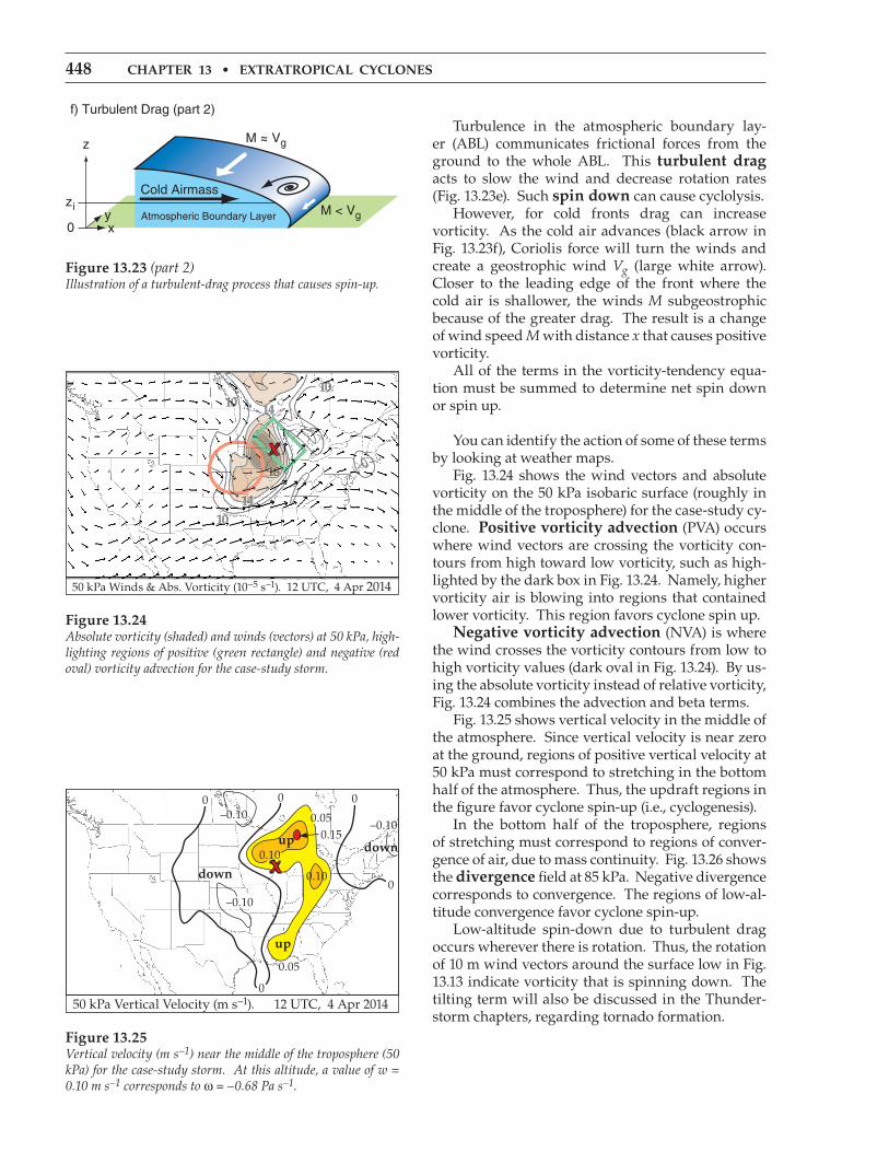
You can identify the action of some of these terms by looking at weather maps. Fig. 13.24 shows the wind vectors and absolute vorticity on the 50 kPa isobaric surface (roughly in the middle of the troposphere) for the case-study cy-clone. positive vorticity advection (PVA) occurs where wind vectors are crossing the vorticity con-tours from high toward low vorticity, such as high-lighted by the dark box in Fig. 13.24. Namely, higher vorticity air is blowing into regions that contained lower vorticity. This region favors cyclone spin up. negative vorticity advection (NVA) is where the wind crosses the vorticity contours from low to high vorticity values (dark oval in Fig. 13.24). By us-ing the absolute vorticity instead of relative vorticity, Fig. 13.24 combines the advection and beta terms. Fig. 13.25 shows vertical velocity in the middle of the atmosphere. Since vertical velocity is near zero at the ground, regions of positive vertical velocity at 50 kPa must correspond to stretching in the bottom half of the atmosphere. Thus, the updraft regions in the figure favor cyclone spin-up (i.e., cyclogenesis). In the bottom half of the troposphere, regions of stretching must correspond to regions of conver-gence of air, due to mass continuity. Fig. 13.26 shows the divergence field at 85 kPa. Negative divergence corresponds to convergence. The regions of low-al-titude convergence favor cyclone spin-up. Low-altitude spin-down due to turbulent drag occurs wherever there is rotation. Thus, the rotation of 10 m wind vectors around the surface low in Fig. 13.13 indicate vorticity that is spinning down. The tilting term will also be discussed in the Thunder-storm chapters, regarding tornado formation.
Figure 13.25Vertical velocity (m s–1) near the middle of the troposphere (50 kPa) for the case-study storm. At this altitude, a value of w = 0.10 m s–1 corresponds to ω = –0.68 Pa s–1.
Figure 13.24Absolute vorticity (shaded) and winds (vectors) at 50 kPa, high-lighting regions of positive (green rectangle) and negative (red oval) vorticity advection for the case-study storm.
50 kPa Winds & Abs. Vorticity (10–5 s–1). 12 UTC, 4 Apr 2014
x
50 kPa Vertical Velocity (m s–1). 12 UTC, 4 Apr 2014
0.05
0.05
up
up
00
0
0
0
0.15
0.10
0.10
–0.10
–0.10–0.10
down
down
x
Figure 13.23 (part 2)Illustration of a turbulent-drag process that causes spin-up.
r. stull • practical MEtEorology 449
Quasi-Geostrophic approximation Above the boundary layer (and away from fronts, jets, and thunderstorms) the terms in the second line of the vorticity equation are smaller than those in the first line, and can be neglected. Also, for syn-optic scale, extratropical weather systems, the winds are almost geostrophic (quasi-geostrophic). These weather phenomena are simpler to ana-lyze than thunderstorms and hurricanes, and can be well approximated by a set of equations (quasi-geo-strophic vorticity and omega equations) that are less complicated than the full set of primitive equa-tions of motion (Newton’s second law, the first law of thermodynamics, continuity, and ideal gas law). As a result of the simplifications above, the vorticity forecast equation simplifies to the follow-ing quasi-geostrophic vorticity equation:
•(13.10)
∆∆
= −∆∆
−∆∆
−∆∆
+ζ ζ ζg
gg
gg
gc
ctU
xV
yV
fy
f ∆∆∆Wz
spin-up horizontal advection beta stretching
where the relative geostrophic vorticity ζg is defined similar to the relative vorticity of eq. (11.20), except using geostrophic winds Ug and Vg:
ζgg gV
x
U
y=∆∆
−∆∆
•(13.11)
For solid body rotation, eq. (11.22) becomes:
ζgG
R=
2 · •(13.12)
where G is the geostrophic wind speed and R is the radius of curvature. The prefix “quasi-” is used for the following rea-sons. If the winds were perfectly geostrophic or gradient, then they would be parallel to the isobars. Such winds never cross the isobars, and could not cause convergence into the low. With no conver-gence there would be no vertical velocity. However, we know from observations that verti-cal motions do exist and are important for causing clouds and precipitation in cyclones. Thus, the last term in the quasi-geostrophic vorticity equation in-cludes W, a wind that is not geostrophic. When such an ageostrophic vertical velocity is included in an equation that otherwise is totally geostrophic, the equation is said to be quasi-geostrophic, meaning partially geostrophic. The quasi-geostrophic ap-proximation will also be used later in this chapter to estimate vertical velocity in cyclones. Within a quasi-geostrophic system, the vorticity and temperature fields are closely coupled, due to
sample application Suppose an initial flow field has no geostrophic relative vorticity, but there is a straight north to south geostrophic wind blowing at 10 m s–1 at latitude 45°. Also, the top of a 1 km thick column of air rises at 0.01 m s–1, while its base rises at 0.008 m s–1. Find the rate of geostrophic-vorticity spin-up.
Find the answerGiven: V = –10 m s–1, ϕ = 45°, Wtop = 0.01 m s–1, Wbottom = 0.008 m s–1, ∆z = 1 km.Find: ∆ζg/∆t = ? s–2
First, get the Coriolis parameter using eq. (10.16): fc = (1.458x10⁻⁴ s–1)·sin(45°) = 0.000103 s–1 Next, use eq. (13.2):
β =
∆∆
= ××
− −fyc 1 458 10
6 357 1045
4
6.
.· cos
s
m
1°
= 1.62x10⁻¹¹ m–1·s–1 Use the definition of a gradient (see Appendix A):
∆∆
=−−
= −Wz
W W
z ztop bottom
top bottom
( . . )0 01 0 008 m//sm( )1000 0−
= 2x10⁻⁶ s–1 Finally, use eq. (13.10). We have no information about advection, so assume it is zero. The remaining terms give:
spin-up beta
∆∆
= − − ×
+
− − −ζg
t( )·( . · )
( .
10 1 62 10
0 0001
11m/s m s1 1
003 2 10 6s s–1 1)·( )× − −
stretching =(1.62x10⁻¹⁰ + 2.06x10⁻¹⁰ ) s–2 = 3.68x10⁻¹⁰ s–2
check: Units OK. Physics OK.Exposition: Even without any initial geostrophic vorticity, the rotation of the Earth can spin-up the flow if the wind blows appropriately.
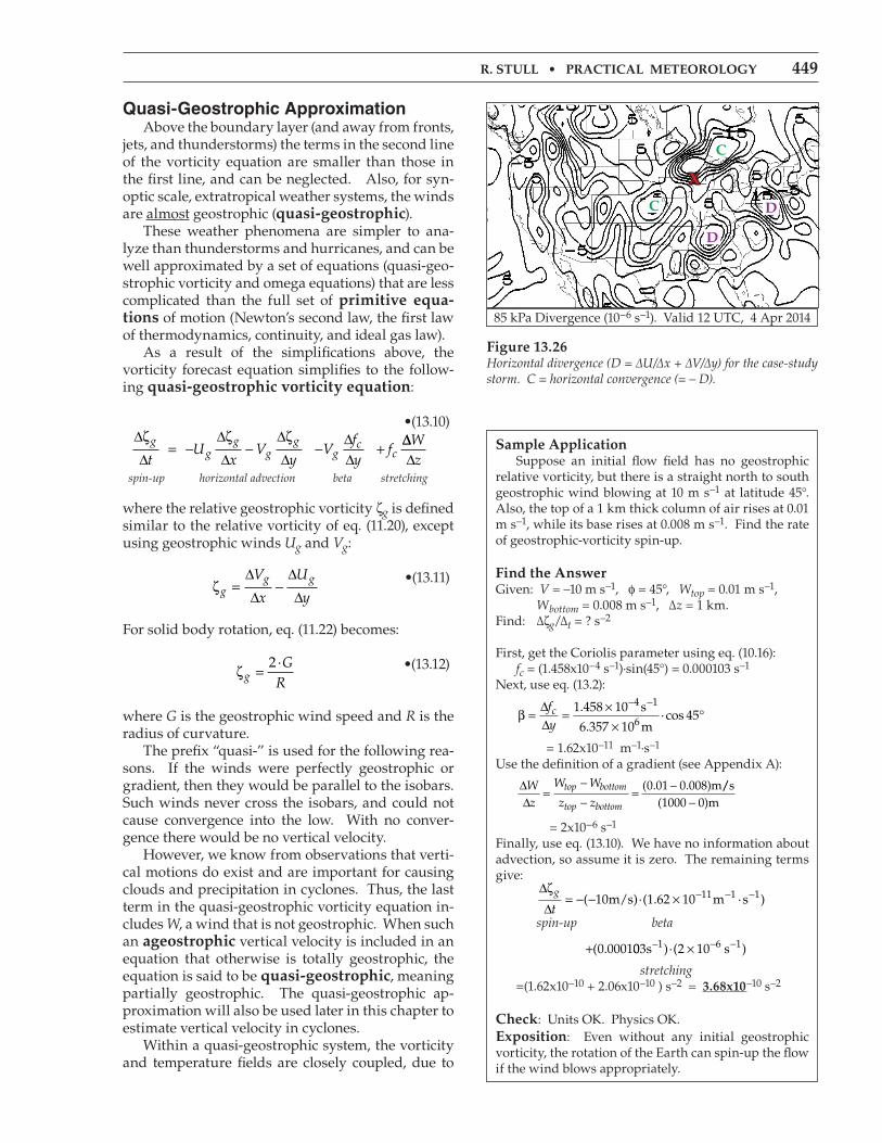
Figure 13.26Horizontal divergence (D = ∆U/∆x + ∆V/∆y) for the case-study storm. C = horizontal convergence (= – D).
85 kPa Divergence (10–6 s–1). Valid 12 UTC, 4 Apr 2014
x
D
D
c
c

450 chaptEr 13 • Extratropical cyclonEs
the dual constraints of geostrophic and hydrostatic balance. This implies close coupling between the wind and mass fields, as was discussed in the Gen-eral Circulation and Fronts chapters in the sections on geostrophic adjustment. While such close cou-pling is not observed for every weather system, it is a reasonable approximation for synoptic-scale, ex-tratropical systems.
application to idealized Weather Pat-
terns An idealized weather pattern (“toy model”) is shown in Fig. 13.27. Every feature in the figure is on the 50 kPa isobaric surface (i.e., in the mid tropo-sphere), except the L which indicates the location of the surface low center. All three components of the geostrophic vorticity equation can be studied. Geostrophic and gradient winds are parallel to the height contours. The trough axis is a region of cyclonic (counterclockwise) curvature of the wind, which yields a large positive value of geostrophic vorticity. At the ridge is negative (clockwise) rela-tive vorticity. Thus, the advection term is positive over the L center and contributes to spin-up of the cyclone because the wind is blowing higher positive vorticity into the area of the surface low. For any fixed pressure gradient, the gradient winds are slower than geostrophic when curving cy-clonically (“slow around lows”), and faster than geo-strophic for anticyclonic curvature, as sketched with the thick-line wind arrows in Fig. 13.27. Examine the 50 kPa flow immediately above the surface low. Air is departing faster than entering. This imbal-ance (divergence) draws air up from below. Hence, W increases from near zero at the ground to some positive updraft speed at 50 kPa. This stretching helps to spin-up the cyclone. The beta term, however, contributes to spin-down because air from lower latitudes (with smaller Coriolis parameter) is blowing toward the location of the surface cyclone. This effect is small when the wave amplitude is small. The sum of all three terms in the quasigeostrophic vorticity equation is often positive, providing a net spin-up and intensification of the cyclone. In real cyclones, contours are often more closely spaced in troughs, causing relative maxima in jet stream winds called jet streaks. Vertical motions as-sociated with horizontal divergence in jet streaks are discussed later in this chapter. These motions vio-late the assumption that air mass is conserved along an “isobaric channel”. Rossby also pointed out in 1940 that the gradient wind balance is not valid for varying motions. Thus, the “toy” model of Fig. 13.27 has weaknesses that limit its applicability.
Figure 13.27An idealized 50 kPa chart with equally-spaced height contours, as introduced by J. Bjerknes in 1937. The location of the surface low L is indicated.
hiGher Math • the laplacian
A Laplacian operator ∇2 can be defined as
∇ = ∂∂
+ ∂∂
+ ∂∂
22
2
2
2
2
2AA
x
A
y
A
zwhere A represents any variable. Sometimes we are concerned only with the horizontal (H) portion:
∇ = ∂∂
+ ∂∂H A
A
x
A
y2
2
2
2
2( )
What does it mean? If ∂A/∂x represents the slope of a line when A is plotted vs. x on a graph, then ∂2A/∂x2 = ∂[ ∂A/∂x ]/∂x is the change of slope; namely, the curvature. How is it used? Recall from the Atm. Forces & Winds chapter that the geostrophic wind is defined as U
f ygc
= − ∂∂
1 Φ V
f xgc
= ∂∂
1 Φ
where Φ is the geopotential ( Φ = |g|·z ). Plugging these into eq. (13.11) gives the geostrophic vorticity:
ζg
c cx f x y f y= ∂∂
∂∂
+ ∂∂
∂∂
1 1Φ Φ
or
ζgc
Hf= ∇1 2 ( )Φ (13.11b)
This illustrates the value of the Laplacian — as a way to more concisely describe the physics. For example, a low-pressure center corresponds to a low-height center on an isobaric sfc. That isobaric surface is concave up, which corresponds to positive curvature. Namely, the Laplacian of |g|·z is positive,hence, ζg is positive. Thus, a low has positive vorticity. Figure f.
r. stull • practical MEtEorology 451
asCent
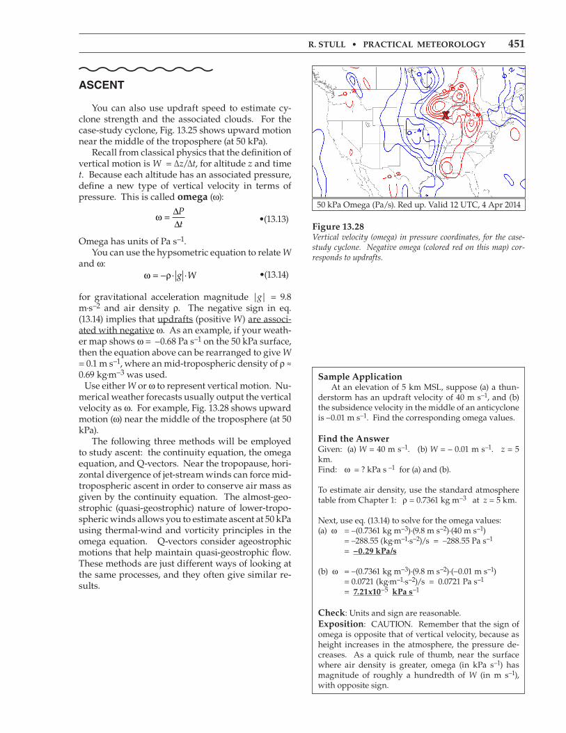
You can also use updraft speed to estimate cy-clone strength and the associated clouds. For the case-study cyclone, Fig. 13.25 shows upward motion near the middle of the troposphere (at 50 kPa). Recall from classical physics that the definition of vertical motion is W = ∆z/∆t, for altitude z and time t. Because each altitude has an associated pressure, define a new type of vertical velocity in terms of pressure. This is called omega (ω):
ω = ∆∆Pt •(13.13)
Omega has units of Pa s–1. You can use the hypsometric equation to relate W and ω: ω ρ= − · ·g W •(13.14)
for gravitational acceleration magnitude |g| = 9.8 m·s–2 and air density ρ. The negative sign in eq. (13.14) implies that updrafts (positive W) are associ-ated with negative ω. As an example, if your weath-er map shows ω = –0.68 Pa s–1 on the 50 kPa surface, then the equation above can be rearranged to give W = 0.1 m s–1, where an mid-tropospheric density of ρ ≈ 0.69 kg·m–3 was used. Use either W or ω to represent vertical motion. Nu-merical weather forecasts usually output the vertical velocity as ω. For example, Fig. 13.28 shows upward motion (ω) near the middle of the troposphere (at 50 kPa). The following three methods will be employed to study ascent: the continuity equation, the omega equation, and Q-vectors. Near the tropopause, hori-zontal divergence of jet-stream winds can force mid-tropospheric ascent in order to conserve air mass as given by the continuity equation. The almost-geo-strophic (quasi-geostrophic) nature of lower-tropo-spheric winds allows you to estimate ascent at 50 kPa using thermal-wind and vorticity principles in the omega equation. Q-vectors consider ageostrophic motions that help maintain quasi-geostrophic flow. These methods are just different ways of looking at the same processes, and they often give similar re-sults.
sample application At an elevation of 5 km MSL, suppose (a) a thun-derstorm has an updraft velocity of 40 m s–1, and (b) the subsidence velocity in the middle of an anticyclone is –0.01 m s–1. Find the corresponding omega values.
Find the answerGiven: (a) W = 40 m s–1. (b) W = – 0.01 m s–1. z = 5 km.Find: ω = ? kPa s –1 for (a) and (b).
To estimate air density, use the standard atmosphere table from Chapter 1: ρ = 0.7361 kg m–3 at z = 5 km.
Next, use eq. (13.14) to solve for the omega values:(a) ω = –(0.7361 kg m–3)·(9.8 m s–2)·(40 m s–1) = –288.55 (kg·m–1·s–2)/s = –288.55 Pa s–1 = –0.29 kpa/s
(b) ω = –(0.7361 kg m–3)·(9.8 m s–2)·(–0.01 m s–1) = 0.0721 (kg·m–1·s–2)/s = 0.0721 Pa s–1 = 7.21x10⁻⁵ kpa s–1
check: Units and sign are reasonable.Exposition: CAUTION. Remember that the sign of omega is opposite that of vertical velocity, because as height increases in the atmosphere, the pressure de-creases. As a quick rule of thumb, near the surface where air density is greater, omega (in kPa s–1) has magnitude of roughly a hundredth of W (in m s–1), with opposite sign.
Figure 13.28Vertical velocity (omega) in pressure coordinates, for the case-study cyclone. Negative omega (colored red on this map) cor-responds to updrafts.
50 kPa Omega (Pa/s). Red up. Valid 12 UTC, 4 Apr 2014
x
452 chaptEr 13 • Extratropical cyclonEs
Continuity effects horizontal divergence (D = ∆U/∆x + ∆V/∆y) is where more air leaves a volume than enters, horizon-tally. This can occur at locations where jet-stream wind speed (Mout) exiting a volume is greater than entrance speeds (Min). Conservation of air mass requires that the num-ber of air molecules in a volume, such as the light blue region sketched in Fig. 13.29, must remain near-ly constant (neglecting compressibility). Namely, volume inflow must balance volume outflow of air. Net vertical inflow can compensate for net hori-zontal outflow. In the troposphere, most of this in-flow happens a mid-levels (P ≈ 50 kPa) as an upward vertical velocity (Wmid). Not much vertical inflow happens across the tropopause because vertical mo-tion in the stratosphere is suppressed by the strong static stability. In the idealized illustration of Fig. 13.29, the inflows [(Min times the area across which the inflow occurs) plus (Wmid times its area of in-flow)] equals the outflow (Mout times the outflow area). The continuity equation describes volume con-servation for this situation as
W D zmid = ·∆ (13.15)
or W
Ux
Vy
zmid = +
∆∆
∆∆
·∆ (13.16)
or
WMs
zmid = ∆∆
∆· (13.17)
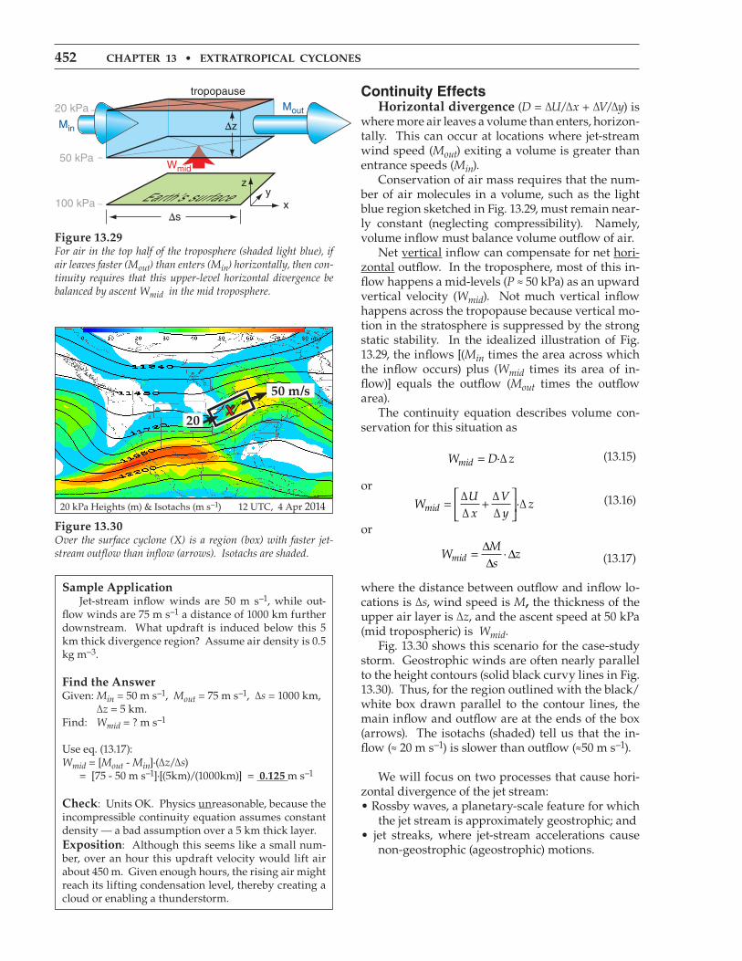
where the distance between outflow and inflow lo-cations is ∆s, wind speed is M, the thickness of the upper air layer is ∆z, and the ascent speed at 50 kPa (mid tropospheric) is Wmid. Fig. 13.30 shows this scenario for the case-study storm. Geostrophic winds are often nearly parallel to the height contours (solid black curvy lines in Fig. 13.30). Thus, for the region outlined with the black/white box drawn parallel to the contour lines, the main inflow and outflow are at the ends of the box (arrows). The isotachs (shaded) tell us that the in-flow (≈ 20 m s–1) is slower than outflow (≈50 m s–1).
We will focus on two processes that cause hori-zontal divergence of the jet stream: • Rossby waves, a planetary-scale feature for which
the jet stream is approximately geostrophic; and • jet streaks, where jet-stream accelerations cause
non-geostrophic (ageostrophic) motions.
sample application Jet-stream inflow winds are 50 m s–1, while out-flow winds are 75 m s–1 a distance of 1000 km further downstream. What updraft is induced below this 5 km thick divergence region? Assume air density is 0.5 kg m–3.
Find the answerGiven: Min = 50 m s–1, Mout = 75 m s–1, ∆s = 1000 km, ∆z = 5 km.Find: Wmid = ? m s–1
Use eq. (13.17):Wmid = [Mout - Min]·(∆z/∆s) = [75 - 50 m s–1]·[(5km)/(1000km)] = 0.125 m s–1
check: Units OK. Physics unreasonable, because the incompressible continuity equation assumes constant density — a bad assumption over a 5 km thick layer.Exposition: Although this seems like a small num-ber, over an hour this updraft velocity would lift air about 450 m. Given enough hours, the rising air might reach its lifting condensation level, thereby creating a cloud or enabling a thunderstorm.
Figure 13.30Over the surface cyclone (X) is a region (box) with faster jet-stream outflow than inflow (arrows). Isotachs are shaded.
20 kPa Heights (m) & Isotachs (m s–1) 12 UTC, 4 Apr 2014
x20
50 m/s
Figure 13.29For air in the top half of the troposphere (shaded light blue), if air leaves faster (Mout) than enters (Min) horizontally, then con-tinuity requires that this upper-level horizontal divergence be balanced by ascent Wmid in the mid troposphere.
r. stull • practical MEtEorology 453
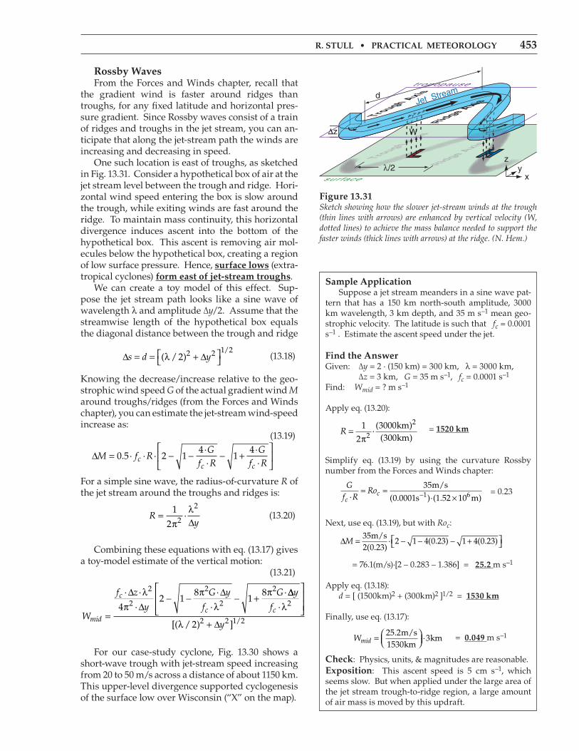
rossby Waves From the Forces and Winds chapter, recall that the gradient wind is faster around ridges than troughs, for any fixed latitude and horizontal pres-sure gradient. Since Rossby waves consist of a train of ridges and troughs in the jet stream, you can an-ticipate that along the jet-stream path the winds are increasing and decreasing in speed. One such location is east of troughs, as sketched in Fig. 13.31. Consider a hypothetical box of air at the jet stream level between the trough and ridge. Hori-zontal wind speed entering the box is slow around the trough, while exiting winds are fast around the ridge. To maintain mass continuity, this horizontal divergence induces ascent into the bottom of the hypothetical box. This ascent is removing air mol-ecules below the hypothetical box, creating a region of low surface pressure. Hence, surface lows (extra-tropical cyclones) form east of jet-stream troughs. We can create a toy model of this effect. Sup-pose the jet stream path looks like a sine wave of wavelength λ and amplitude ∆y/2. Assume that the streamwise length of the hypothetical box equals the diagonal distance between the trough and ridge
∆ = = + ∆
s d y( / )
/λ 2 2 2 1 2
(13.18)
Knowing the decrease/increase relative to the geo-strophic wind speed G of the actual gradient wind M around troughs/ridges (from the Forces and Winds chapter), you can estimate the jet-stream wind-speed increase as: (13.19)
∆ = − − − +
M f R
Gf R
Gf Rc
c c0 5 2 1
41
4. · · ·
··
··
For a simple sine wave, the radius-of-curvature R of the jet stream around the troughs and ridges is:
Ry
=π ∆1
2 2
2·λ
(13.20)
Combining these equations with eq. (13.17) gives a toy-model estimate of the vertical motion: (13.21)
W
f z
y
G y
f
G
mid
c
c=
∆π ∆
− −π ∆
− +π· ·
·
·
·
·λλ
2
2
2
2
2
42 1
81
8 ∆∆
+ ∆
y
f
y
c ·
[( / ) ] /
λ
λ
2
2 2 1 22
For our case-study cyclone, Fig. 13.30 shows a short-wave trough with jet-stream speed increasing from 20 to 50 m/s across a distance of about 1150 km. This upper-level divergence supported cyclogenesis of the surface low over Wisconsin (“X” on the map).
sample application Suppose a jet stream meanders in a sine wave pat-tern that has a 150 km north-south amplitude, 3000 km wavelength, 3 km depth, and 35 m s–1 mean geo-strophic velocity. The latitude is such that fc = 0.0001 s–1 . Estimate the ascent speed under the jet.
Find the answerGiven: ∆y = 2 · (150 km) = 300 km, λ = 3000 km, ∆z = 3 km, G = 35 m s–1, fc = 0.0001 s–1
Find: Wmid = ? m s–1
Apply eq. (13.20):
R =π1
2
30003002
2·( )
( )kmkm
= 1520 km
Simplify eq. (13.19) by using the curvature Rossby number from the Forces and Winds chapter:
G
f RRo
cc· ( . )·( . )
= =×−
35
0 0001 1 52 10
m/s
s m1 6 = 0.23
Next, use eq. (13.19), but with Roc:
∆ = − − − + M352 0 23
2 1 4 0 23 1 4 0 23m/s
( . )· ( . ) ( . )
= 76.1(m/s)·[2 – 0.283 – 1.386] = 25.2 m s–1
Apply eq. (13.18): d = [ (1500km)2 + (300km)2 ]1/2 = 1530 km
Finally, use eq. (13.17):
Wmid =
25 21530
3.
·m/skm
km = 0.049 m s–1
check: Physics, units, & magnitudes are reasonable.Exposition: This ascent speed is 5 cm s–1, which seems slow. But when applied under the large area of the jet stream trough-to-ridge region, a large amount of air mass is moved by this updraft.
Figure 13.31Sketch showing how the slower jet-stream winds at the trough (thin lines with arrows) are enhanced by vertical velocity (W, dotted lines) to achieve the mass balance needed to support the faster winds (thick lines with arrows) at the ridge. (N. Hem.)
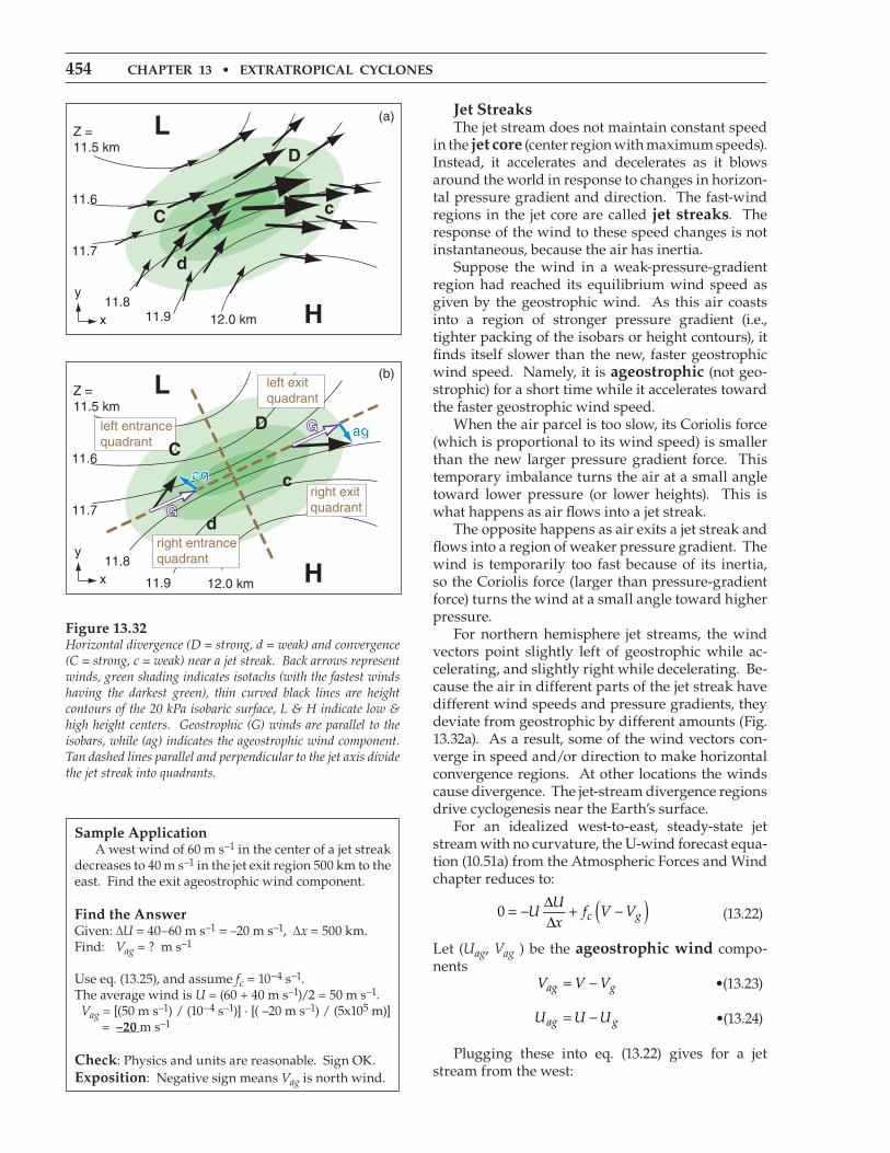
454 chaptEr 13 • Extratropical cyclonEs
Jet streaks The jet stream does not maintain constant speed in the jet core (center region with maximum speeds). Instead, it accelerates and decelerates as it blows around the world in response to changes in horizon-tal pressure gradient and direction. The fast-wind regions in the jet core are called jet streaks. The response of the wind to these speed changes is not instantaneous, because the air has inertia. Suppose the wind in a weak-pressure-gradient region had reached its equilibrium wind speed as given by the geostrophic wind. As this air coasts into a region of stronger pressure gradient (i.e., tighter packing of the isobars or height contours), it finds itself slower than the new, faster geostrophic wind speed. Namely, it is ageostrophic (not geo-strophic) for a short time while it accelerates toward the faster geostrophic wind speed. When the air parcel is too slow, its Coriolis force (which is proportional to its wind speed) is smaller than the new larger pressure gradient force. This temporary imbalance turns the air at a small angle toward lower pressure (or lower heights). This is what happens as air flows into a jet streak. The opposite happens as air exits a jet streak and flows into a region of weaker pressure gradient. The wind is temporarily too fast because of its inertia, so the Coriolis force (larger than pressure-gradient force) turns the wind at a small angle toward higher pressure. For northern hemisphere jet streams, the wind vectors point slightly left of geostrophic while ac-celerating, and slightly right while decelerating. Be-cause the air in different parts of the jet streak have different wind speeds and pressure gradients, they deviate from geostrophic by different amounts (Fig. 13.32a). As a result, some of the wind vectors con-verge in speed and/or direction to make horizontal convergence regions. At other locations the winds cause divergence. The jet-stream divergence regions drive cyclogenesis near the Earth’s surface. For an idealized west-to-east, steady-state jet stream with no curvature, the U-wind forecast equa-tion (10.51a) from the Atmospheric Forces and Wind chapter reduces to:
0 = − ∆∆
+ −( )UUx
f V Vc g (13.22)
Let (Uag, Vag ) be the ageostrophic wind compo-nents V V Vag g= − •(13.23)
U U Uag g= − •(13.24)
Plugging these into eq. (13.22) gives for a jet stream from the west:
sample application A west wind of 60 m s–1 in the center of a jet streak decreases to 40 m s–1 in the jet exit region 500 km to the east. Find the exit ageostrophic wind component.
Find the answerGiven: ∆U = 40–60 m s–1 = –20 m s–1, ∆x = 500 km.Find: Vag = ? m s–1
Use eq. (13.25), and assume fc = 10–4 s–1. The average wind is U = (60 + 40 m s–1)/2 = 50 m s–1. Vag = [(50 m s–1) / (10–4 s–1)] · [( –20 m s–1) / (5x10⁵ m)] = –20 m s–1
check: Physics and units are reasonable. Sign OK. Exposition: Negative sign means Vag is north wind.
Figure 13.32Horizontal divergence (D = strong, d = weak) and convergence (C = strong, c = weak) near a jet streak. Back arrows represent winds, green shading indicates isotachs (with the fastest winds having the darkest green), thin curved black lines are height contours of the 20 kPa isobaric surface, L & H indicate low & high height centers. Geostrophic (G) winds are parallel to the isobars, while (ag) indicates the ageostrophic wind component. Tan dashed lines parallel and perpendicular to the jet axis divide the jet streak into quadrants.
r. stull • practical MEtEorology 455
VUf
Uxag
c= ∆
∆· •(13.25)
Similarly, the ageostrophic wind for south-to-north jet stream axis is
UVf
Vyag
c= − ∆
∆· •(13.26)
For example, consider the winds approaching the jet streak (i.e., in the entrance region) in Fig. 13.32a. The air moves into a region where U is positive and increases with x, hence Vag is positive according to eq. (13.25). Also, V is positive and increases with y, hence, Uag is negative. The resulting ageostrophic entrance vector is shown in blue in Fig. 13.32b. Simi-lar analyses can be made for the jet-streak exit re-gions, yielding the corresponding ageostrophic wind component. When considering a jet streak, imagine it divided into the four quadrants sketched in Fig. 13.32 (also Fig. 13.35). The combination of speed and direc-tion changes cause strong divergence in the left exit quadrant, and weaker divergence in the right entrance quadrant. These are the regions where cyclogenesis is favored under the jet. Cyclolysis is favored under the convergence regions of the right exit and left entrance regions. This ageostrophic behavior can also be seen in the maps for a different case-study (Fig. 13.33). This fig-ure overlays wind vectors, isotachs, and geopotential height contours near the top of the troposphere (at 20 kPa). The broad area of shading shows the jet stream. Embedded within it are two relative speed maxima (one over Texas, and the other over New England) that we identify as jet streaks. Recall that if winds are geostrophic (or gradient), then they should flow parallel to the height contours. In Fig. 13.33 the square highlights the exit region of the Texas jet streak, showing wind vectors that cross the height contours toward the right. Name-ly, inertia has caused these winds to be faster than geostrophic (supergeostrophic), therefore Coriolis force is stronger than pressure-gradient force, caus-ing the winds to be to the right of geostrophic. The oval highlights the entrance region of the second jet, where winds cross the height contours to the left. Inertia results in slower-than-geostrophic winds (subgeostrophic), causing the Coriolis force to be too weak to counteract pressure-gradient force. Consider a vertical slice through the atmosphere, perpendicular to the geostrophic wind at the jet exit region (Fig. 13.32). The resulting combination of ageostrophic winds (Mag) induce mid-tropospheric ascent (Wmid) and descent that favors cyclogenesis and cyclolysis, respectively (Fig. 13.34). The weak, vertical, cross-jet flow (orange in Fig. 13.34) is a sec-ondary circulation.
inFo • ageostrophic right-hand rule
If the geostrophic winds are accelerating, use your right hand to curl your fingers from vertical toward the direction of acceleration (theacceleration vector). Your thumbpoints in the direction of the ageostrophic wind. This right-hand rule also works for deceleration, for which case the direction of acceleration is opposite
to the wind direction. Figure g.
Figure 13.33 (not the 2014 case study.)Superposition of the 20 kPa charts for geopotential heights (me-dium-thickness black curved lines), isotachs in m s–1 (shading), and winds (vectors). The scale for winds and the values for the height contours are identical to those in Figs. 13.17. Regions of relatively darker shading indicate the jet streaks. White/black square outlines the exit region from a small jet streak over Texas, and white/black oval outlines the entrance region for a larger jet streak over the northeastern USA.
Figure 13.34Vertical slice through the atmosphere at the jet-streak exit re-gion, perpendicular to the average jet direction. Viewed from the west southwest, the green shading indicates isotachs of the jet core into the page. Divergence (D) in the left exit region creates ascent (W, dotted lines) to conserve air mass, which in turn removes air from near the surface. This causes the surface pressure to drop, favoring cyclogenesis. The opposite happens under the right exit region, where cyclolysis is favored.
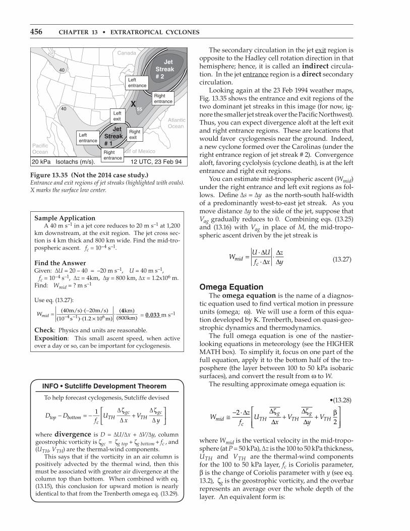
456 chaptEr 13 • Extratropical cyclonEs
The secondary circulation in the jet exit region is opposite to the Hadley cell rotation direction in that hemisphere; hence, it is called an indirect circula-tion. In the jet entrance region is a direct secondary circulation. Looking again at the 23 Feb 1994 weather maps, Fig. 13.35 shows the entrance and exit regions of the two dominant jet streaks in this image (for now, ig-nore the smaller jet streak over the Pacific Northwest). Thus, you can expect divergence aloft at the left exit and right entrance regions. These are locations that would favor cyclogenesis near the ground. Indeed, a new cyclone formed over the Carolinas (under the right entrance region of jet streak # 2). Convergence aloft, favoring cyclolysis (cyclone death), is at the left entrance and right exit regions. You can estimate mid-tropospheric ascent (Wmid) under the right entrance and left exit regions as fol-lows. Define ∆s = ∆y as the north-south half-width of a predominantly west-to-east jet streak. As you move distance ∆y to the side of the jet, suppose that Vag gradually reduces to 0. Combining eqs. (13.25) and (13.16) with Vag in place of M, the mid-tropo-spheric ascent driven by the jet streak is
WU Uf x
zymid
c=
∆∆
∆∆
··
· (13.27)
omega equation The omega equation is the name of a diagnos-tic equation used to find vertical motion in pressure units (omega; ω). We will use a form of this equa-tion developed by K. Trenberth, based on quasi-geo-strophic dynamics and thermodynamics. The full omega equation is one of the nastier-looking equations in meteorology (see the HIGHER MATH box). To simplify it, focus on one part of the full equation, apply it to the bottom half of the tro-posphere (the layer between 100 to 50 kPa isobaric surfaces), and convert the result from ω to W. The resulting approximate omega equation is:
•(13.28)
W
zf
Ux
Vy
Vmidc
THg
THg
TH≅−
+ +
22
·∆ ∆∆
∆∆
ζ ζ β
where Wmid is the vertical velocity in the mid-tropo-sphere (at P = 50 kPa), ∆z is the 100 to 50 kPa thickness, UTH and VTH are the thermal-wind components for the 100 to 50 kPa layer, fc is Coriolis parameter, β is the change of Coriolis parameter with y (see eq. 13.2), ζg is the geostrophic vorticity, and the overbar represents an average over the whole depth of the layer. An equivalent form is:
sample application A 40 m s–1 in a jet core reduces to 20 m s–1 at 1,200 km downstream, at the exit region. The jet cross sec-tion is 4 km thick and 800 km wide. Find the mid-tro-pospheric ascent. fc = 10–4 s–1.
Find the answerGiven: ∆U = 20 – 40 = –20 m s–1, U = 40 m s–1, fc = 10–4 s–1, ∆z = 4km, ∆y = 800 km, ∆x = 1.2x10⁶ m.Find: Wmid = ? m s–1
Use eq. (13.27):
Wmid =−×− −
( )·( )
( )·( . )·
(40 20
10 1 2 104 6m/s m/s
s m144
800kmkm
)( ) = 0.033 m s–1
check: Physics and units are reasonable.Exposition: This small ascent speed, when active over a day or so, can be important for cyclogenesis.
Figure 13.35 (not the 2014 case study.)Entrance and exit regions of jet streaks (highlighted with ovals). X marks the surface low center.
inFo • sutcliffe development theorem
To help forecast cyclogenesis, Sutcliffe devised
D D
fU
xV
ytop bottomc
THgc
THgc− = − +
1 ∆
∆
∆
∆
ζ ζ
where divergence is D = ∆U/∆x + ∆V/∆y, column geostrophic vorticity is ζgc = ζg top + ζg bottom + fc , and (UTH, VTH) are the thermal-wind components. This says that if the vorticity in an air column is positively advected by the thermal wind, then this must be associated with greater air divergence at the column top than bottom. When combined with eq. (13.15), this conclusion for upward motion is nearly identical to that from the Trenberth omega eq. (13.29).
r. stull • practical MEtEorology 457
W
zf
Mf
smidc
THg c
≅− +( )
2 2· ( / )∆ ∆
∆
ζ •(13.29)
where s is distance along the thermal wind direc-tion, and MTH is the thermal-wind speed. Regardless of the form, the terms in square brack-ets represent the advection of vorticity by the ther-mal wind, where vorticity consists of the geostroph-ic relative vorticity plus a part of the vorticity due to the Earth’s rotation. The geostrophic vorticity at the 85 kPa or the 70 kPa isobaric surface is often used to approximate the average geostrophic vorticity over the whole 100 to 50 kPa layer. A physical interpretation of the omega equation is that greater upward velocity occurs where there is greater advection of cyclonic (positive) geostrophic vorticity by the thermal wind. Greater upward ve-locity favors clouds and heavier precipitation. Also, by moving air upward from the surface, it reduces the pressure under it, causing the surface low to move toward that location and deepen. Weather maps can be used to determine the loca-tion and magnitude of the maximum upward mo-tion. The idealized map of Fig. 13.36a shows the height (z) contours of the 50 kPa isobaric surface, along with the trough axis. Also shown is the loca-tion of the surface low and fronts. At the surface, the greatest vorticity is often near the low center. At 50 kPa, it is often near the trough axis. At 70 kPa, the vorticity maximum (vort max) is usually between those two locations. In Fig. 13.36a, the darker shading corresponds to regions of greater cyclonic vorticity at 70 kPa. Fig. 13.36b shows the thickness (∆z) of the layer of air between the 100 and 50 kPa isobaric surfaces. Thickness lines are often nearly parallel to surface fronts, with the tightest packing on the cold side of the fronts. Recall that thermal wind is parallel to the thickness lines, with cold air to the left, and with the greatest velocity where the thickness lines are most tightly packed. Thermal wind direction is represented by the arrows in Fig. 13.36b, with longer arrows denoting stronger speed. Advection is greatest where the area between crossing isopleths is smallest (the INFO Box on the next page explains why). This rule also works for advection by the thermal wind. The dotted lines represent the isopleths that drive the thermal wind. In Fig. 13.36 the thin black lines around the shaded areas are isopleths of vorticity. The solenoid at the smallest area between these crossing isopleths indi-cates the greatest vorticity advection by the thermal wind, and is outlined by a rectangular box. For this
Figure 13.36(a) Weather at three different pressure heights: (1) 50 kPa heights (solid lines) and trough axis (thick dashed line); (2) surface low pressure center (L) and fronts; (3) 70 kPa vorticity (shaded).(b) Trough axis, surface low and fronts, and vorticity shading are identical to Fig. (a). Added are: 100 to 50 kPa thickness (dotted lines), thermal wind vectors (arrows), and region of maximum positive vorticity advection by the thermal wind (rectangular box). It is within this box that the omega equation gives the greatest updraft speed, which support cyclogenesis.
sample application The 100 to 50 kPa thickness is 5 km and fc = 10–4 s–1. A west to east thermal wind of 20 m s–1 blows through a region where avg. cyclonic vorticity decreases by 10–4 s–1 toward the east across a distance of 500 km. Use the omega eq. to find mid-tropospheric upward speed.
Find the answerGiven: UTH = 20 m s–1, VTH = 0, ∆z = 5 km, ∆ζ = –10–4 s–1 , ∆x = 500 km, fc = 10–4 s–1.Find: Wmid = ? m s–1
Use eq. (13.28):
Wmid ≅− −
− −
− −2 5000
1020
10
54
4·( )
( )( )
( )
(
m
sm/s
s1
1
××+ +
10
0 05 m) = 0.4 m
s–1
check: Units OK. Physics OK.Exposition: At this speed, an air parcel would take 7.6 h to travel from the ground to the tropopause.
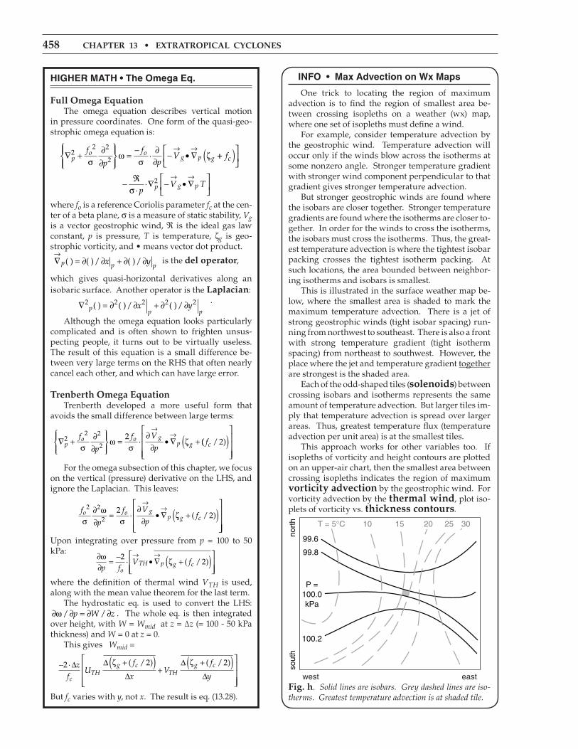
458 chaptEr 13 • Extratropical cyclonEs
hiGher Math • the omega eq.
Full omega Equation The omega equation describes vertical motion in pressure coordinates. One form of the quasi-geo-strophic omega equation is:
∇ + ∂∂
=− ∂
∂− • ∇→ →
po o
g p gf
p
fp
V22 2
2σω
σζ· ++( )
− ℜ ∇ − • ∇
→ →
f
pV T
c
p g pσ ·· 2
where fo is a reference Coriolis parameter fc at the cen-ter of a beta plane, σ is a measure of static stability, Vg is a vector geostrophic wind, ℜ is the ideal gas law constant, p is pressure, T is temperature, ζg is geo-strophic vorticity, and • means vector dot product. ∇ = ∂ ∂ + ∂ ∂→
p p px y( ) ( )/ ( )/ is the del operator,
which gives quasi-horizontal derivatives along an isobaric surface. Another operator is the laplacian: ∇ = ∂ ∂ + ∂ ∂2 2 2 2 2
p p px y( ) ( )/ ( )/
.
Although the omega equation looks particularly complicated and is often shown to frighten unsus-pecting people, it turns out to be virtually useless. The result of this equation is a small difference be-tween very large terms on the RHS that often nearly cancel each other, and which can have large error.
trenberth omega Equation Trenberth developed a more useful form that avoids the small difference between large terms:
∇ + ∂∂
=
∂∂
• ∇ +
→→
po o g
p gf
p
f V
p2
2 2
22
σω
σζ· (( / )fc 2( )
For the omega subsection of this chapter, we focus on the vertical (pressure) derivative on the LHS, and ignore the Laplacian. This leaves:
f
p
f V
pfo o g
p g c
2 2
22
2σ
ωσ
ζ∂∂
=∂∂
• ∇ +( )
→→
· ( / )
Upon integrating over pressure from p = 100 to 50 kPa:
∂∂
= − • ∇ +( )
→ →ω ζp f
V fo
TH p g c2
2· ( / )
where the definition of thermal wind VTH is used, along with the mean value theorem for the last term. The hydrostatic eq. is used to convert the LHS: ∂ ∂ = ∂ ∂ω/ /p W z . The whole eq. is then integrated over height, with W = Wmid at z = ∆z (= 100 - 50 kPa thickness) and W = 0 at z = 0. This gives Wmid =
− +( )+
+( )2 2 2· ( / ) ( / )∆ ∆
∆
∆
∆z
fU
f
xV
f
ycTH
g cTH
g cζ ζ
But fc varies with y, not x. The result is eq. (13.28).
inFo • Max advection on Wx Maps
One trick to locating the region of maximum advection is to find the region of smallest area be-tween crossing isopleths on a weather (wx) map, where one set of isopleths must define a wind. For example, consider temperature advection by the geostrophic wind. Temperature advection will occur only if the winds blow across the isotherms at some nonzero angle. Stronger temperature gradient with stronger wind component perpendicular to that gradient gives stronger temperature advection. But stronger geostrophic winds are found where the isobars are closer together. Stronger temperature gradients are found where the isotherms are closer to-gether. In order for the winds to cross the isotherms, the isobars must cross the isotherms. Thus, the great-est temperature advection is where the tightest isobar packing crosses the tightest isotherm packing. At such locations, the area bounded between neighbor-ing isotherms and isobars is smallest. This is illustrated in the surface weather map be-low, where the smallest area is shaded to mark the maximum temperature advection. There is a jet of strong geostrophic winds (tight isobar spacing) run-ning from northwest to southeast. There is also a front with strong temperature gradient (tight isotherm spacing) from northeast to southwest. However, the place where the jet and temperature gradient together are strongest is the shaded area. Each of the odd-shaped tiles (solenoids) between crossing isobars and isotherms represents the same amount of temperature advection. But larger tiles im-ply that temperature advection is spread over larger areas. Thus, greatest temperature flux (temperature advection per unit area) is at the smallest tiles. This approach works for other variables too. If isopleths of vorticity and height contours are plotted on an upper-air chart, then the smallest area between crossing isopleths indicates the region of maximum vorticity advection by the geostrophic wind. For vorticity advection by the thermal wind, plot iso-plets of vorticity vs. thickness contours.
Fig. h. Solid lines are isobars. Grey dashed lines are iso-therms. Greatest temperature advection is at shaded tile.
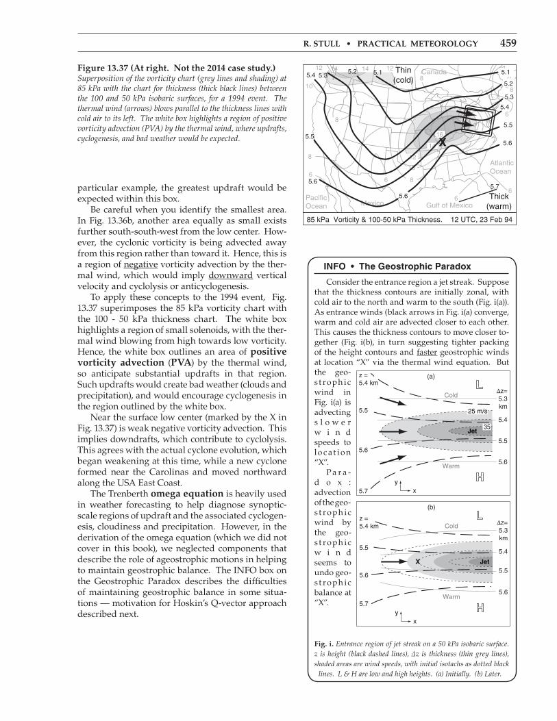
r. stull • practical MEtEorology 459
particular example, the greatest updraft would be expected within this box. Be careful when you identify the smallest area. In Fig. 13.36b, another area equally as small exists further south-south-west from the low center. How-ever, the cyclonic vorticity is being advected away from this region rather than toward it. Hence, this is a region of negative vorticity advection by the ther-mal wind, which would imply downward vertical velocity and cyclolysis or anticyclogenesis. To apply these concepts to the 1994 event, Fig. 13.37 superimposes the 85 kPa vorticity chart with the 100 - 50 kPa thickness chart. The white box highlights a region of small solenoids, with the ther-mal wind blowing from high towards low vorticity. Hence, the white box outlines an area of positive vorticity advection (pVa) by the thermal wind, so anticipate substantial updrafts in that region. Such updrafts would create bad weather (clouds and precipitation), and would encourage cyclogenesis in the region outlined by the white box. Near the surface low center (marked by the X in Fig. 13.37) is weak negative vorticity advection. This implies downdrafts, which contribute to cyclolysis. This agrees with the actual cyclone evolution, which began weakening at this time, while a new cyclone formed near the Carolinas and moved northward along the USA East Coast. The Trenberth omega equation is heavily used in weather forecasting to help diagnose synoptic-scale regions of updraft and the associated cyclogen-esis, cloudiness and precipitation. However, in the derivation of the omega equation (which we did not cover in this book), we neglected components that describe the role of ageostrophic motions in helping to maintain geostrophic balance. The INFO box on the Geostrophic Paradox describes the difficulties of maintaining geostrophic balance in some situa-tions — motivation for Hoskin’s Q-vector approach described next.
Figure 13.37 (at right. not the 2014 case study.)Superposition of the vorticity chart (grey lines and shading) at 85 kPa with the chart for thickness (thick black lines) between the 100 and 50 kPa isobaric surfaces, for a 1994 event. The thermal wind (arrows) blows parallel to the thickness lines with cold air to its left. The white box highlights a region of positive vorticity advection (PVA) by the thermal wind, where updrafts, cyclogenesis, and bad weather would be expected.
inFo • the Geostrophic Paradox
Consider the entrance region a jet streak. Suppose that the thickness contours are initially zonal, with cold air to the north and warm to the south (Fig. i(a)). As entrance winds (black arrows in Fig. i(a) converge, warm and cold air are advected closer to each other. This causes the thickness contours to move closer to-gether (Fig. i(b), in turn suggesting tighter packing of the height contours and faster geostrophic winds at location “X” via the thermal wind equation. But the geo-s t roph ic wind in Fig. i(a) is advecting s l o w e r w i n d speeds to lo c at io n “X”. P a r a -d o x : advection of the geo-s t r oph ic wind by the geo-s t r oph ic w i n d seems to undo geo-s t r oph ic balance at “X”.
Fig. i. Entrance region of jet streak on a 50 kPa isobaric surface. z is height (black dashed lines), ∆z is thickness (thin grey lines), shaded areas are wind speeds, with initial isotachs as dotted black
lines. L & H are low and high heights. (a) Initially. (b) Later.
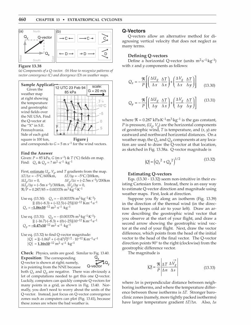
460 chaptEr 13 • Extratropical cyclonEs
Q-vectors Q-vectors allow an alternative method for di-agnosing vertical velocity that does not neglect as many terms.
Defining Q-vectors Define a horizontal Q-vector (units m2·s–1·kg–1) with x and y components as follows:
Q
P
U
xTx
V
xTyx
g g= − ℜ
+
·
∆
∆·∆∆
∆
∆·∆∆
(13.30)
Q
P
U
yTx
V
yTyy
g g= − ℜ
+
·
∆
∆·∆∆
∆
∆·∆∆
(13.31)
where ℜ = 0.287 kPa·K–1·m3·kg–1 is the gas constant, P is pressure, (Ug, Vg) are the horizontal components of geostrophic wind, T is temperature, and (x, y) are eastward and northward horizontal distances. On a weather map, the Qx and Qy components at any loca-tion are used to draw the Q-vector at that location, as sketched in Fig. 13.38a. Q-vector magnitude is
Q Q Qx y= +( )2 2 1 2/ (13.32)
Estimating Q-vectors Eqs. (13.30 - 13.32) seem non-intuitive in their ex-isting Cartesian form. Instead, there is an easy way to estimate Q-vector direction and magnitude using weather maps. First, look at direction. Suppose you fly along an isotherm (Fig. 13.39) in the direction of the thermal wind (in the direc-tion that keeps cold air to your left). Draw an ar-row describing the geostrophic wind vector that you observe at the start of your flight, and draw a second arrow showing the geostrophic wind vec-tor at the end of your flight. Next, draw the vector difference, which points from the head of the initial vector to the head of the final vector. The Q-vector direction points 90° to the right (clockwise) from the geostrophic difference vector. The magnitude is
QP
Tn
V
sg= ℜ
→∆∆
·∆
∆ (13.33)
where ∆n is perpendicular distance between neigh-boring isotherms, and where the temperature differ-ence between those isotherms is ∆T. Stronger baro-clinic zones (namely, more tightly packed isotherms) have larger temperature gradient ∆T/∆n. Also, ∆s
sample application Given theweather mapat right showingthe temperatureand geostrophicwind fields overthe NE USA. Findthe Q-vector atthe “X” in S.E.Pennsylvania.Side of each grid square is 100 km, Figure jand corresponds to G = 5 m s–1 for the wind vectors.
Find the answerGiven: P = 85 kPa, G (m s–1) & T (°C) fields on map.Find: Qx & Qy = ? m2 ·s–1 ·kg–1
First, estimate Ug, Vg, and T gradients from the map.∆T/∆x = –5°C/600km, ∆T/∆y = –5°C/200km, ∆Ug/∆x = 0, ∆Vg/∆x = (–2.5m s–1)/200km∆Ug/∆y = (–5m s–1)/300km, ∆Vg/∆y = 0,ℜ/P = 0.287/85 = 0.003376 m3·kg–1·K–1
Use eq. (13.30): Qx = – (0.003376 m3·kg–1·K–1)· [( (0)·(–8.3) + (–12.5)·(–25)]·10–12 K·m–1·s–1 Qx = –1.06x10⁻¹² m2 ·s–1 ·kg–1
Use eq. (13.31): Qy = – (0.003376 m3·kg–1·K–1)· [( (–16.7)·(–8.3) + (0)·(–25)]·10–12 K·m–1·s–1 Qy = –0.47x10⁻¹² m2 ·s–1 ·kg–1
Use eq. (13.32) to find Q-vector magnitude: |Q| = [(–1.06)2 + (–0.47)2]1/2 · 10–12 K·m–1·s–1
|Q| = 1.16x10⁻¹² m2 ·s–1 ·kg–1
check: Physics, units are good. Similar to Fig. 13.40.Exposition: The correspondingQ-vector is shown at right; namely,it is pointing from the NNE because both Qx and Qy are negative. There was obviously a lot of computations needed to get this one Q-vector. Luckily, computers can quickly compute Q-vectors for many points in a grid, as shown in Fig. 13.40. Nor-mally, you don’t need to worry about the units of the Q-vector. Instead, just focus on Q-vector convergence zones such as computers can plot (Fig. 13.41), because these zones are where the bad weather is.
Figure 13.38(a) Components of a Q-vector. (b) How to recognize patterns of vector convergence (C) and divergence (D) on weather maps.
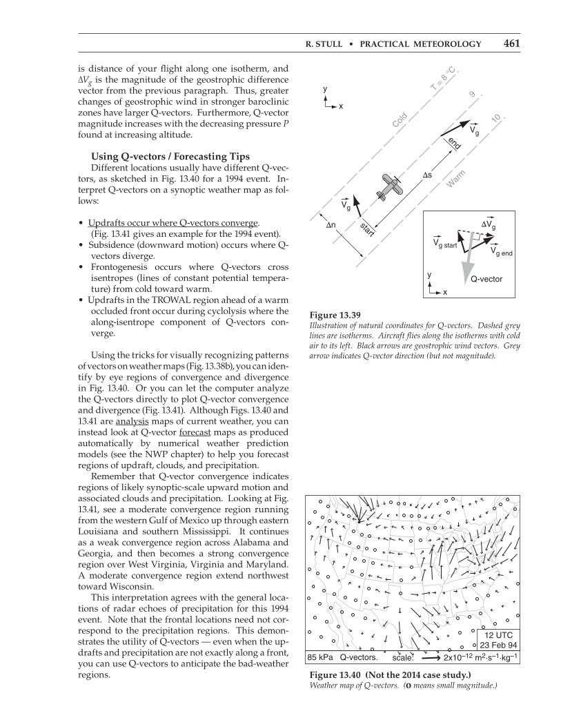
r. stull • practical MEtEorology 461
is distance of your flight along one isotherm, and ∆Vg is the magnitude of the geostrophic difference vector from the previous paragraph. Thus, greater changes of geostrophic wind in stronger baroclinic zones have larger Q-vectors. Furthermore, Q-vector magnitude increases with the decreasing pressure P found at increasing altitude.
using Q-vectors / Forecasting tips Different locations usually have different Q-vec-tors, as sketched in Fig. 13.40 for a 1994 event. In-terpret Q-vectors on a synoptic weather map as fol-lows:
• Updrafts occur where Q-vectors converge. (Fig. 13.41 gives an example for the 1994 event).• Subsidence (downward motion) occurs where Q-
vectors diverge.• Frontogenesis occurs where Q-vectors cross
isentropes (lines of constant potential tempera-ture) from cold toward warm.
• Updrafts in the TROWAL region ahead of a warm occluded front occur during cyclolysis where the along-isentrope component of Q-vectors con-verge.
Using the tricks for visually recognizing patterns of vectors on weather maps (Fig. 13.38b), you can iden-tify by eye regions of convergence and divergence in Fig. 13.40. Or you can let the computer analyze the Q-vectors directly to plot Q-vector convergence and divergence (Fig. 13.41). Although Figs. 13.40 and 13.41 are analysis maps of current weather, you can instead look at Q-vector forecast maps as produced automatically by numerical weather prediction models (see the NWP chapter) to help you forecast regions of updraft, clouds, and precipitation. Remember that Q-vector convergence indicates regions of likely synoptic-scale upward motion and associated clouds and precipitation. Looking at Fig. 13.41, see a moderate convergence region running from the western Gulf of Mexico up through eastern Louisiana and southern Mississippi. It continues as a weak convergence region across Alabama and Georgia, and then becomes a strong convergence region over West Virginia, Virginia and Maryland. A moderate convergence region extend northwest toward Wisconsin. This interpretation agrees with the general loca-tions of radar echoes of precipitation for this 1994 event. Note that the frontal locations need not cor-respond to the precipitation regions. This demon-strates the utility of Q-vectors — even when the up-drafts and precipitation are not exactly along a front, you can use Q-vectors to anticipate the bad-weather regions. Figure 13.40 (not the 2014 case study.)
Weather map of Q-vectors. (o means small magnitude.)
Figure 13.39Illustration of natural coordinates for Q-vectors. Dashed grey lines are isotherms. Aircraft flies along the isotherms with cold air to its left. Black arrows are geostrophic wind vectors. Grey arrow indicates Q-vector direction (but not magnitude).
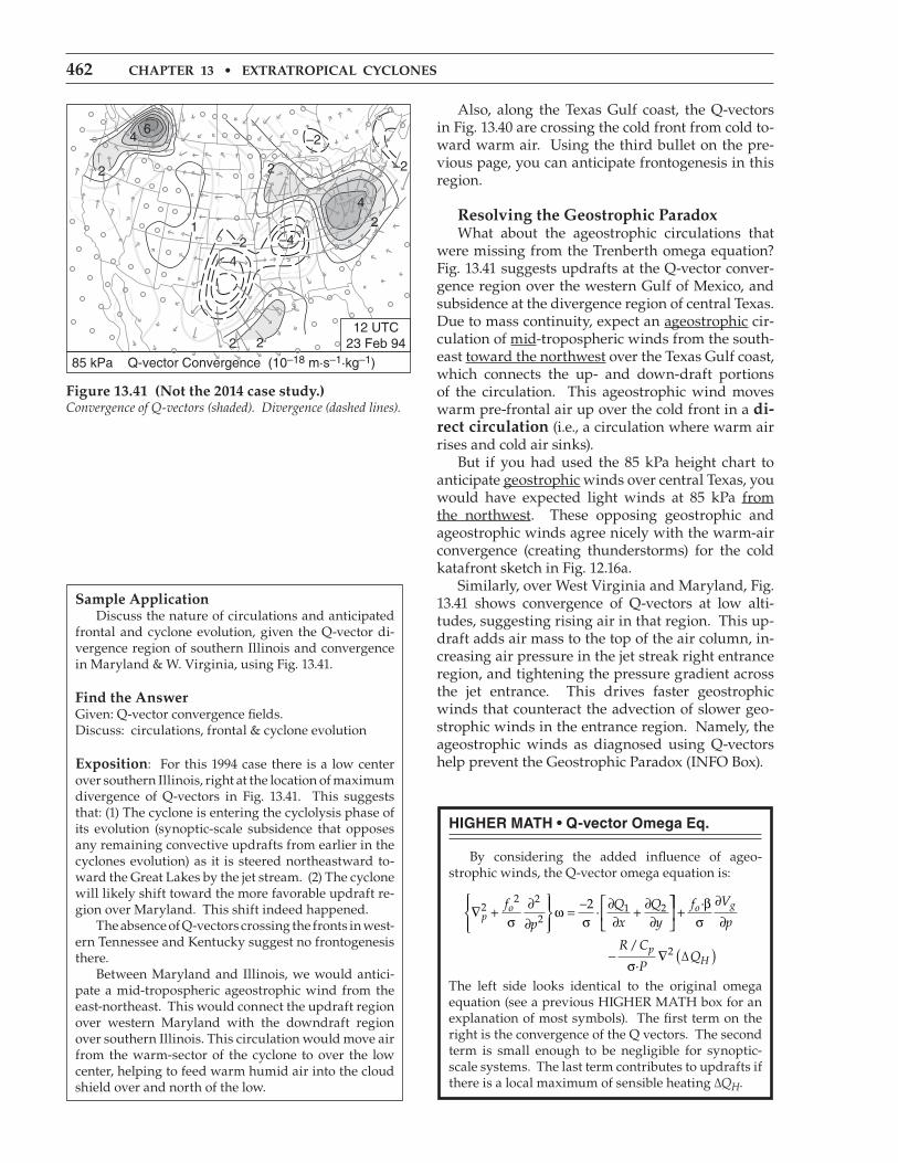
462 chaptEr 13 • Extratropical cyclonEs
Also, along the Texas Gulf coast, the Q-vectors in Fig. 13.40 are crossing the cold front from cold to-ward warm air. Using the third bullet on the pre-vious page, you can anticipate frontogenesis in this region.
resolving the geostrophic paradox What about the ageostrophic circulations that were missing from the Trenberth omega equation? Fig. 13.41 suggests updrafts at the Q-vector conver-gence region over the western Gulf of Mexico, and subsidence at the divergence region of central Texas. Due to mass continuity, expect an ageostrophic cir-culation of mid-tropospheric winds from the south-east toward the northwest over the Texas Gulf coast, which connects the up- and down-draft portions of the circulation. This ageostrophic wind moves warm pre-frontal air up over the cold front in a di-rect circulation (i.e., a circulation where warm air rises and cold air sinks). But if you had used the 85 kPa height chart to anticipate geostrophic winds over central Texas, you would have expected light winds at 85 kPa from the northwest. These opposing geostrophic and ageostrophic winds agree nicely with the warm-air convergence (creating thunderstorms) for the cold katafront sketch in Fig. 12.16a. Similarly, over West Virginia and Maryland, Fig. 13.41 shows convergence of Q-vectors at low alti-tudes, suggesting rising air in that region. This up-draft adds air mass to the top of the air column, in-creasing air pressure in the jet streak right entrance region, and tightening the pressure gradient across the jet entrance. This drives faster geostrophic winds that counteract the advection of slower geo-strophic winds in the entrance region. Namely, the ageostrophic winds as diagnosed using Q-vectors help prevent the Geostrophic Paradox (INFO Box).
sample application Discuss the nature of circulations and anticipated frontal and cyclone evolution, given the Q-vector di-vergence region of southern Illinois and convergence in Maryland & W. Virginia, using Fig. 13.41.
Find the answerGiven: Q-vector convergence fields.Discuss: circulations, frontal & cyclone evolution
Exposition: For this 1994 case there is a low center over southern Illinois, right at the location of maximum divergence of Q-vectors in Fig. 13.41. This suggests that: (1) The cyclone is entering the cyclolysis phase of its evolution (synoptic-scale subsidence that opposes any remaining convective updrafts from earlier in the cyclones evolution) as it is steered northeastward to-ward the Great Lakes by the jet stream. (2) The cyclone will likely shift toward the more favorable updraft re-gion over Maryland. This shift indeed happened. The absence of Q-vectors crossing the fronts in west-ern Tennessee and Kentucky suggest no frontogenesis there. Between Maryland and Illinois, we would antici-pate a mid-tropospheric ageostrophic wind from the east-northeast. This would connect the updraft region over western Maryland with the downdraft region over southern Illinois. This circulation would move air from the warm-sector of the cyclone to over the low center, helping to feed warm humid air into the cloud shield over and north of the low.
hiGher Math • Q-vector omega eq.
By considering the added influence of ageo-strophic winds, the Q-vector omega equation is:
∇ + ∂∂
= − ∂
∂+ ∂
∂
p
of
p
Qx
Qy
22 2
21 22
σω
σ·
+
∂∂
− ∇ ( )
f V
p
R C
PQ
o g
pH
·
/
·∆
βσ
σ2
The left side looks identical to the original omega equation (see a previous HIGHER MATH box for an explanation of most symbols). The first term on the right is the convergence of the Q vectors. The second term is small enough to be negligible for synoptic-scale systems. The last term contributes to updrafts if there is a local maximum of sensible heating ∆QH.
Figure 13.41 (not the 2014 case study.)Convergence of Q-vectors (shaded). Divergence (dashed lines).
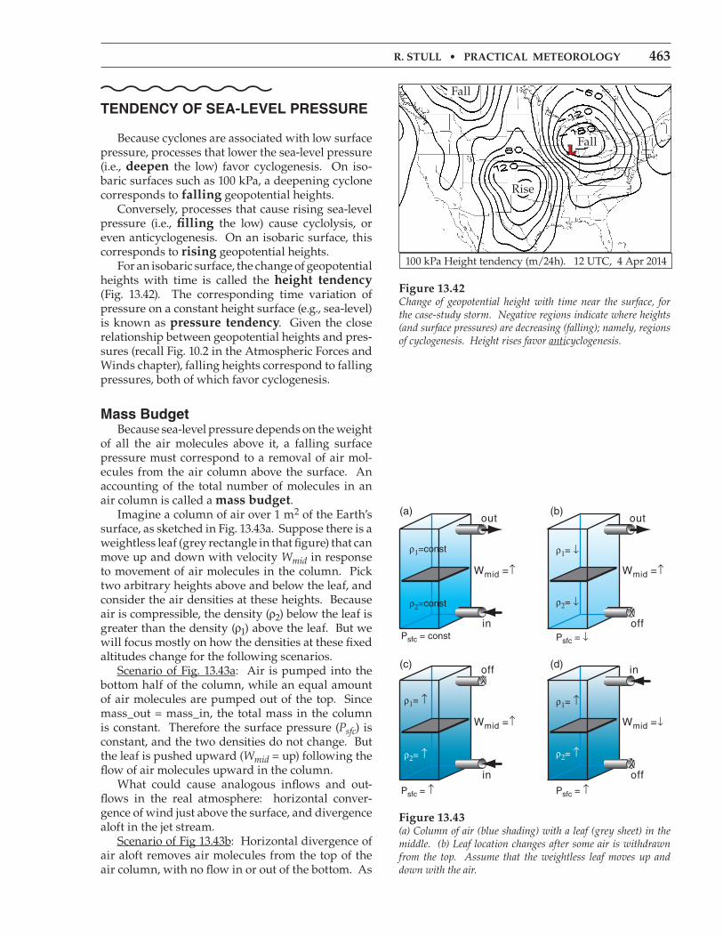
r. stull • practical MEtEorology 463
tendenCy oF sea-level Pressure
Because cyclones are associated with low surface pressure, processes that lower the sea-level pressure (i.e., deepen the low) favor cyclogenesis. On iso-baric surfaces such as 100 kPa, a deepening cyclone corresponds to falling geopotential heights. Conversely, processes that cause rising sea-level pressure (i.e., filling the low) cause cyclolysis, or even anticyclogenesis. On an isobaric surface, this corresponds to rising geopotential heights. For an isobaric surface, the change of geopotential heights with time is called the height tendency (Fig. 13.42). The corresponding time variation of pressure on a constant height surface (e.g., sea-level) is known as pressure tendency. Given the close relationship between geopotential heights and pres-sures (recall Fig. 10.2 in the Atmospheric Forces and Winds chapter), falling heights correspond to falling pressures, both of which favor cyclogenesis.
Mass Budget Because sea-level pressure depends on the weight of all the air molecules above it, a falling surface pressure must correspond to a removal of air mol-ecules from the air column above the surface. An accounting of the total number of molecules in an air column is called a mass budget. Imagine a column of air over 1 m2 of the Earth’s surface, as sketched in Fig. 13.43a. Suppose there is a weightless leaf (grey rectangle in that figure) that can move up and down with velocity Wmid in response to movement of air molecules in the column. Pick two arbitrary heights above and below the leaf, and consider the air densities at these heights. Because air is compressible, the density (ρ2) below the leaf is greater than the density (ρ1) above the leaf. But we will focus mostly on how the densities at these fixed altitudes change for the following scenarios. Scenario of Fig. 13.43a: Air is pumped into the bottom half of the column, while an equal amount of air molecules are pumped out of the top. Since mass_out = mass_in, the total mass in the column is constant. Therefore the surface pressure (Psfc) is constant, and the two densities do not change. But the leaf is pushed upward (Wmid = up) following the flow of air molecules upward in the column. What could cause analogous inflows and out-flows in the real atmosphere: horizontal conver-gence of wind just above the surface, and divergence aloft in the jet stream. Scenario of Fig 13.43b: Horizontal divergence of air aloft removes air molecules from the top of the air column, with no flow in or out of the bottom. As
Figure 13.42Change of geopotential height with time near the surface, for the case-study storm. Negative regions indicate where heights (and surface pressures) are decreasing (falling); namely, regions of cyclogenesis. Height rises favor anticyclogenesis.
100 kPa Height tendency (m/24h). 12 UTC, 4 Apr 2014
lFall
Rise
Fall
Figure 13.43(a) Column of air (blue shading) with a leaf (grey sheet) in the middle. (b) Leaf location changes after some air is withdrawn from the top. Assume that the weightless leaf moves up and down with the air.
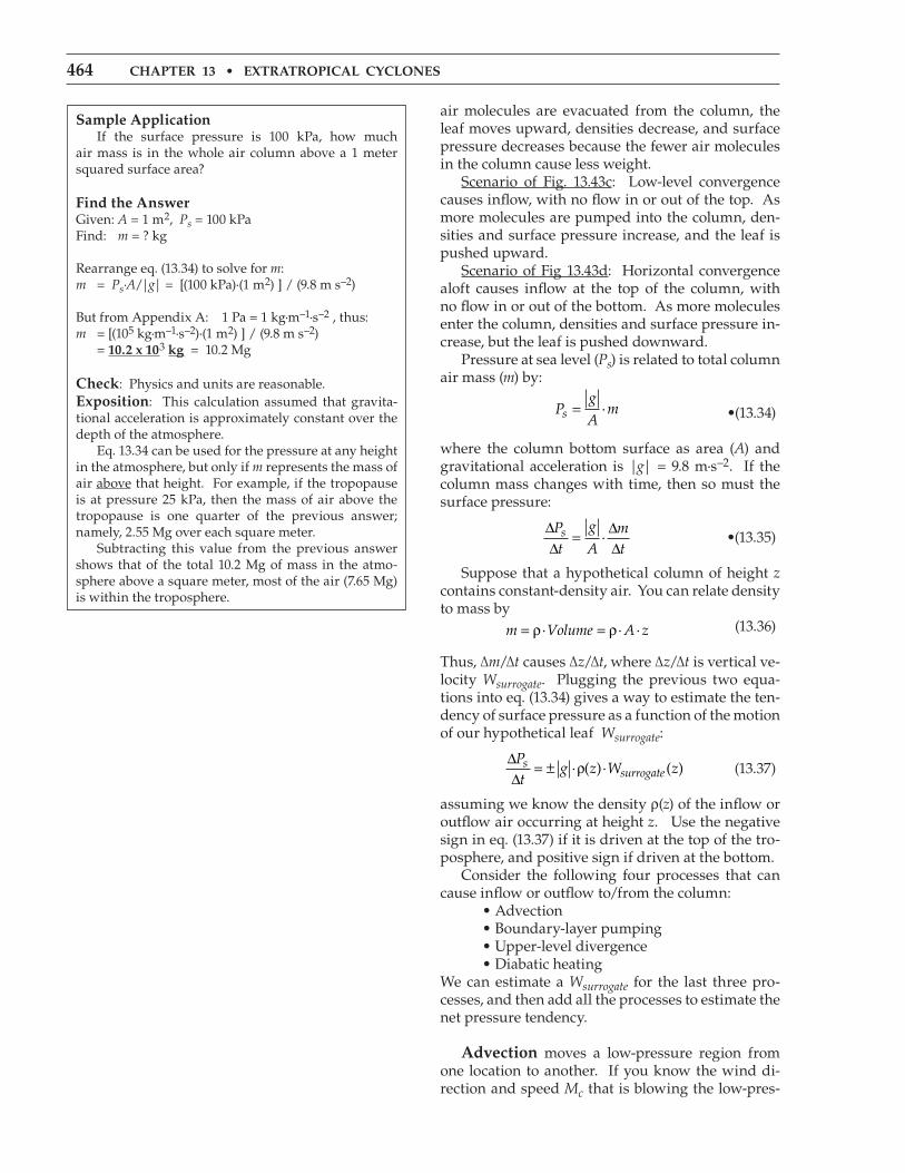
464 chaptEr 13 • Extratropical cyclonEs
air molecules are evacuated from the column, the leaf moves upward, densities decrease, and surface pressure decreases because the fewer air molecules in the column cause less weight. Scenario of Fig. 13.43c: Low-level convergence causes inflow, with no flow in or out of the top. As more molecules are pumped into the column, den-sities and surface pressure increase, and the leaf is pushed upward. Scenario of Fig 13.43d: Horizontal convergence aloft causes inflow at the top of the column, with no flow in or out of the bottom. As more molecules enter the column, densities and surface pressure in-crease, but the leaf is pushed downward. Pressure at sea level (Ps) is related to total column air mass (m) by:
Pg
Ams = · •(13.34)
where the column bottom surface as area (A) and gravitational acceleration is |g| = 9.8 m·s–2. If the column mass changes with time, then so must the surface pressure:
∆∆
= ∆∆
Pt
g
Amt
s · •(13.35)
Suppose that a hypothetical column of height z contains constant-density air. You can relate density to mass by m Volume A z= =ρ ρ· · · (13.36)
Thus, ∆m/∆t causes ∆z/∆t, where ∆z/∆t is vertical ve-locity Wsurrogate. Plugging the previous two equa-tions into eq. (13.34) gives a way to estimate the ten-dency of surface pressure as a function of the motion of our hypothetical leaf Wsurrogate:
∆∆
= ±Pt
g z W zssurrogate· ( )· ( )ρ (13.37)
assuming we know the density ρ(z) of the inflow or outflow air occurring at height z. Use the negative sign in eq. (13.37) if it is driven at the top of the tro-posphere, and positive sign if driven at the bottom. Consider the following four processes that can cause inflow or outflow to/from the column: • Advection • Boundary-layer pumping • Upper-level divergence • Diabatic heatingWe can estimate a Wsurrogate for the last three pro-cesses, and then add all the processes to estimate the net pressure tendency.
advection moves a low-pressure region from one location to another. If you know the wind di-rection and speed Mc that is blowing the low-pres-
sample application If the surface pressure is 100 kPa, how much air mass is in the whole air column above a 1 meter squared surface area?
Find the answerGiven: A = 1 m2, Ps = 100 kPaFind: m = ? kg
Rearrange eq. (13.34) to solve for m:m = Ps·A/|g| = [(100 kPa)·(1 m2) ] / (9.8 m s–2)
But from Appendix A: 1 Pa = 1 kg·m–1·s–2 , thus:m = [(105 kg·m–1·s–2)·(1 m2) ] / (9.8 m s–2) = 10.2 x 10³ kg = 10.2 Mg
check: Physics and units are reasonable.Exposition: This calculation assumed that gravita-tional acceleration is approximately constant over the depth of the atmosphere. Eq. 13.34 can be used for the pressure at any height in the atmosphere, but only if m represents the mass of air above that height. For example, if the tropopause is at pressure 25 kPa, then the mass of air above the tropopause is one quarter of the previous answer; namely, 2.55 Mg over each square meter. Subtracting this value from the previous answer shows that of the total 10.2 Mg of mass in the atmo-sphere above a square meter, most of the air (7.65 Mg) is within the troposphere.
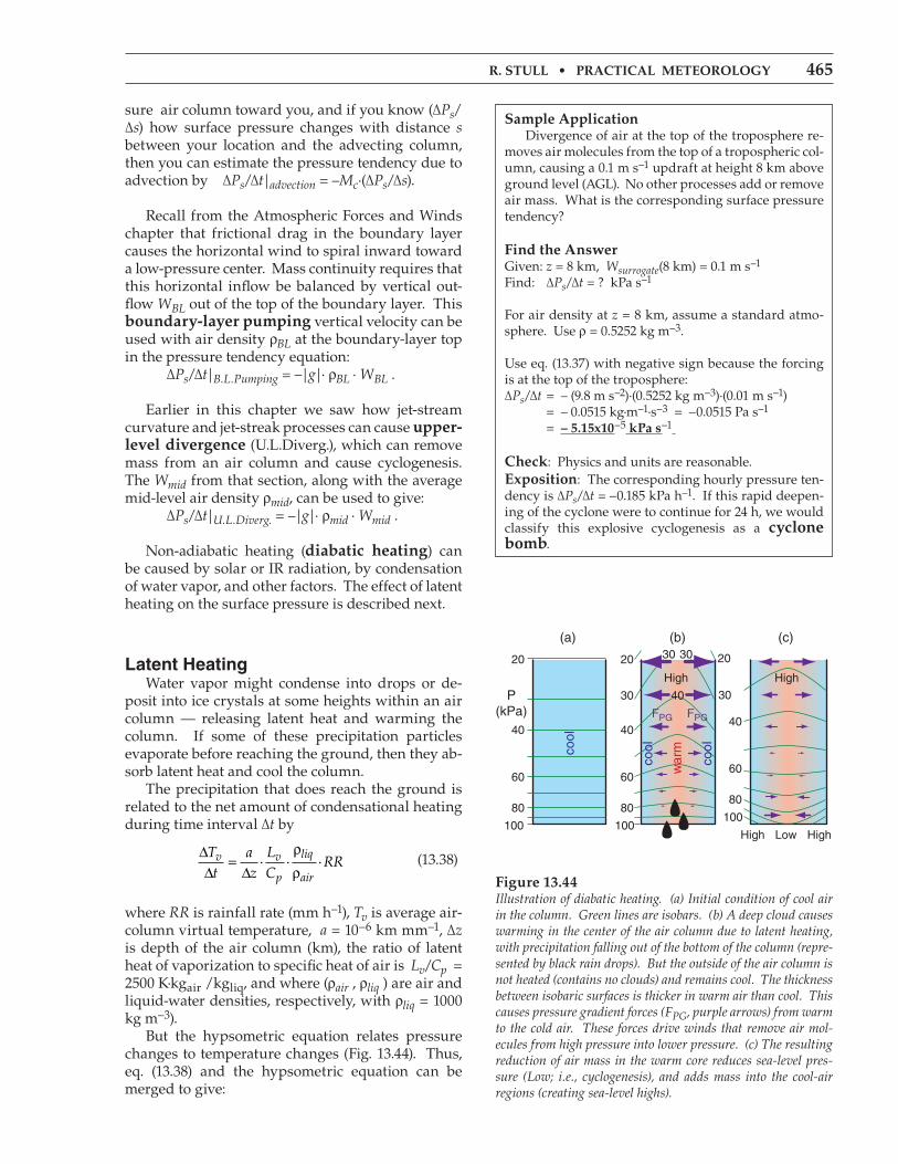
r. stull • practical MEtEorology 465
sure air column toward you, and if you know (∆Ps/∆s) how surface pressure changes with distance s between your location and the advecting column, then you can estimate the pressure tendency due to advection by ∆Ps/∆t|advection = –Mc·(∆Ps/∆s).
Recall from the Atmospheric Forces and Winds chapter that frictional drag in the boundary layer causes the horizontal wind to spiral inward toward a low-pressure center. Mass continuity requires that this horizontal inflow be balanced by vertical out-flow WBL out of the top of the boundary layer. This boundary-layer pumping vertical velocity can be used with air density ρBL at the boundary-layer top in the pressure tendency equation: ∆Ps/∆t|B.L.Pumping = –|g|· ρBL · WBL .
Earlier in this chapter we saw how jet-stream curvature and jet-streak processes can cause upper-level divergence (U.L.Diverg.), which can remove mass from an air column and cause cyclogenesis. The Wmid from that section, along with the average mid-level air density ρmid, can be used to give: ∆Ps/∆t|U.L.Diverg. = –|g|· ρmid · Wmid .
Non-adiabatic heating (diabatic heating) can be caused by solar or IR radiation, by condensation of water vapor, and other factors. The effect of latent heating on the surface pressure is described next.
latent heating Water vapor might condense into drops or de-posit into ice crystals at some heights within an air column — releasing latent heat and warming the column. If some of these precipitation particles evaporate before reaching the ground, then they ab-sorb latent heat and cool the column. The precipitation that does reach the ground is related to the net amount of condensational heating during time interval ∆t by
∆∆
=∆
Tt
az
LC
RRv v
p
liq
air· · ·
ρρ
(13.38)
where RR is rainfall rate (mm h–1), Tv is average air-column virtual temperature, a = 10–6 km mm–1, ∆z is depth of the air column (km), the ratio of latent heat of vaporization to specific heat of air is Lv/Cp = 2500 K·kgair /kgliq, and where (ρair , ρliq ) are air and liquid-water densities, respectively, with ρliq = 1000 kg m–3). But the hypsometric equation relates pressure changes to temperature changes (Fig. 13.44). Thus, eq. (13.38) and the hypsometric equation can be merged to give:
sample application Divergence of air at the top of the troposphere re-moves air molecules from the top of a tropospheric col-umn, causing a 0.1 m s–1 updraft at height 8 km above ground level (AGL). No other processes add or remove air mass. What is the corresponding surface pressure tendency?
Find the answerGiven: z = 8 km, Wsurrogate(8 km) = 0.1 m s–1
Find: ∆Ps/∆t = ? kPa s–1
For air density at z = 8 km, assume a standard atmo-sphere. Use ρ = 0.5252 kg m–3.
Use eq. (13.37) with negative sign because the forcing is at the top of the troposphere:∆Ps/∆t = – (9.8 m s–2)·(0.5252 kg m–3)·(0.01 m s–1) = – 0.0515 kg·m–1·s–3 = –0.0515 Pa s–1 = – 5.15x10⁻⁵ kpa s–1
check: Physics and units are reasonable.Exposition: The corresponding hourly pressure ten-dency is ∆Ps/∆t = –0.185 kPa h–1. If this rapid deepen-ing of the cyclone were to continue for 24 h, we would classify this explosive cyclogenesis as a cyclone bomb.
Figure 13.44Illustration of diabatic heating. (a) Initial condition of cool air in the column. Green lines are isobars. (b) A deep cloud causes warming in the center of the air column due to latent heating, with precipitation falling out of the bottom of the column (repre-sented by black rain drops). But the outside of the air column is not heated (contains no clouds) and remains cool. The thickness between isobaric surfaces is thicker in warm air than cool. This causes pressure gradient forces (FPG, purple arrows) from warm to the cold air. These forces drive winds that remove air mol-ecules from high pressure into lower pressure. (c) The resulting reduction of air mass in the warm core reduces sea-level pres-sure (Low; i.e., cyclogenesis), and adds mass into the cool-air regions (creating sea-level highs).
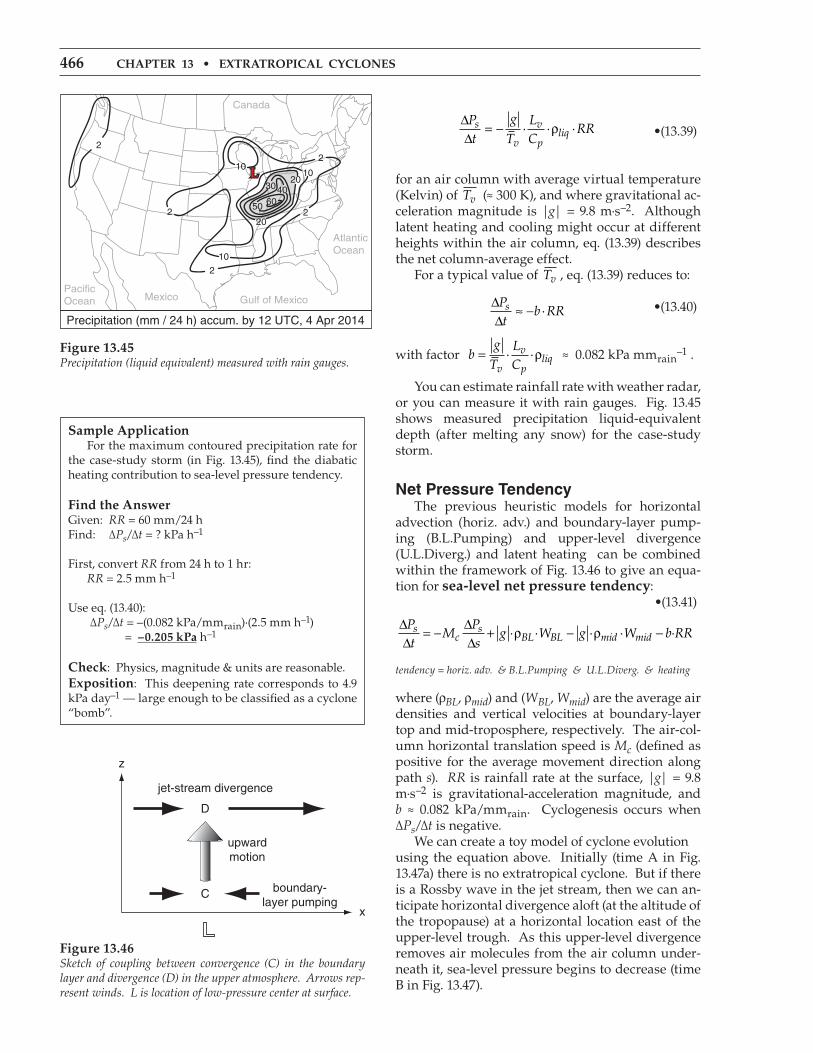
466 chaptEr 13 • Extratropical cyclonEs
∆∆
= −Pt
g
TLC
RRs
v
v
pliq· · ·ρ •(13.39)
for an air column with average virtual temperature (Kelvin) of Tv (≈ 300 K), and where gravitational ac-celeration magnitude is |g| = 9.8 m·s–2. Although latent heating and cooling might occur at different heights within the air column, eq. (13.39) describes the net column-average effect. For a typical value of Tv , eq. (13.39) reduces to:
∆∆
≈ −Pt
b RRs · •(13.40)
with factor bg
TLCv
v
pliq= · ·ρ ≈ 0.082 kPa mmrain
–1 .
You can estimate rainfall rate with weather radar, or you can measure it with rain gauges. Fig. 13.45 shows measured precipitation liquid-equivalent depth (after melting any snow) for the case-study storm.
net Pressure tendency The previous heuristic models for horizontal advection (horiz. adv.) and boundary-layer pump-ing (B.L.Pumping) and upper-level divergence (U.L.Diverg.) and latent heating can be combined within the framework of Fig. 13.46 to give an equa-tion for sea-level net pressure tendency: •(13.41)
∆∆
= −∆∆
+ − −Pt
MPs
g W g W b RRsc
sBL BL mid mid· · · · ·ρ ρ
tendency = horiz. adv. & B.L.Pumping & U.L.Diverg. & heating
where (ρBL, ρmid) and (WBL, Wmid) are the average air densities and vertical velocities at boundary-layer top and mid-troposphere, respectively. The air-col-umn horizontal translation speed is Mc (defined as positive for the average movement direction along path s). RR is rainfall rate at the surface, |g| = 9.8 m·s–2 is gravitational-acceleration magnitude, and b ≈ 0.082 kPa/mmrain. Cyclogenesis occurs when ∆Ps/∆t is negative. We can create a toy model of cyclone evolution using the equation above. Initially (time A in Fig. 13.47a) there is no extratropical cyclone. But if there is a Rossby wave in the jet stream, then we can an-ticipate horizontal divergence aloft (at the altitude of the tropopause) at a horizontal location east of the upper-level trough. As this upper-level divergence removes air molecules from the air column under-neath it, sea-level pressure begins to decrease (time B in Fig. 13.47).
sample application For the maximum contoured precipitation rate for the case-study storm (in Fig. 13.45), find the diabatic heating contribution to sea-level pressure tendency.
Find the answerGiven: RR = 60 mm/24 h Find: ∆Ps/∆t = ? kPa h–1
First, convert RR from 24 h to 1 hr: RR = 2.5 mm h–1 Use eq. (13.40): ∆Ps/∆t = –(0.082 kPa/mmrain)·(2.5 mm h–1) = –0.205 kpa h–1
check: Physics, magnitude & units are reasonable.Exposition: This deepening rate corresponds to 4.9 kPa day–1 — large enough to be classified as a cyclone “bomb”.
Figure 13.46Sketch of coupling between convergence (C) in the boundary layer and divergence (D) in the upper atmosphere. Arrows rep-resent winds. L is location of low-pressure center at surface.
Figure 13.45Precipitation (liquid equivalent) measured with rain gauges.
l
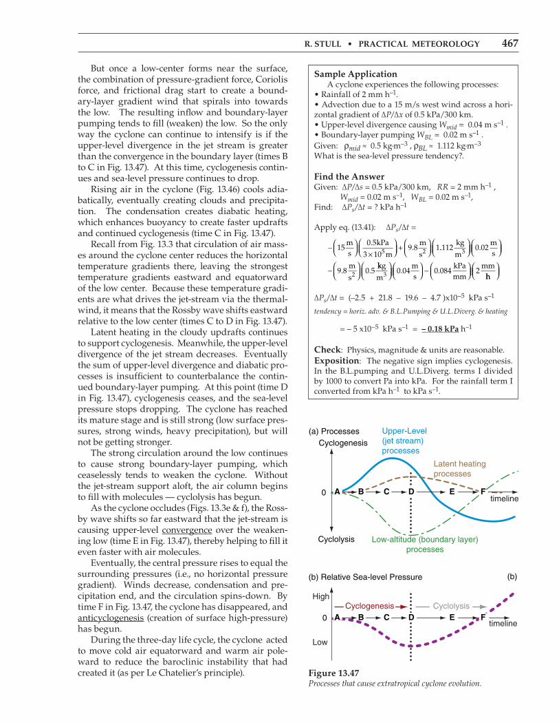
r. stull • practical MEtEorology 467
But once a low-center forms near the surface, the combination of pressure-gradient force, Coriolis force, and frictional drag start to create a bound-ary-layer gradient wind that spirals into towards the low. The resulting inflow and boundary-layer pumping tends to fill (weaken) the low. So the only way the cyclone can continue to intensify is if the upper-level divergence in the jet stream is greater than the convergence in the boundary layer (times B to C in Fig. 13.47). At this time, cyclogenesis contin-ues and sea-level pressure continues to drop. Rising air in the cyclone (Fig. 13.46) cools adia-batically, eventually creating clouds and precipita-tion. The condensation creates diabatic heating, which enhances buoyancy to create faster updrafts and continued cyclogenesis (time C in Fig. 13.47). Recall from Fig. 13.3 that circulation of air mass-es around the cyclone center reduces the horizontal temperature gradients there, leaving the strongest temperature gradients eastward and equatorward of the low center. Because these temperature gradi-ents are what drives the jet-stream via the thermal-wind, it means that the Rossby wave shifts eastward relative to the low center (times C to D in Fig. 13.47). Latent heating in the cloudy updrafts continues to support cyclogenesis. Meanwhile, the upper-level divergence of the jet stream decreases. Eventually the sum of upper-level divergence and diabatic pro-cesses is insufficient to counterbalance the contin-ued boundary-layer pumping. At this point (time D in Fig. 13.47), cyclogenesis ceases, and the sea-level pressure stops dropping. The cyclone has reached its mature stage and is still strong (low surface pres-sures, strong winds, heavy precipitation), but will not be getting stronger. The strong circulation around the low continues to cause strong boundary-layer pumping, which ceaselessly tends to weaken the cyclone. Without the jet-stream support aloft, the air column begins to fill with molecules — cyclolysis has begun. As the cyclone occludes (Figs. 13.3e & f), the Ross-by wave shifts so far eastward that the jet-stream is causing upper-level convergence over the weaken-ing low (time E in Fig. 13.47), thereby helping to fill it even faster with air molecules. Eventually, the central pressure rises to equal the surrounding pressures (i.e., no horizontal pressure gradient). Winds decrease, condensation and pre-cipitation end, and the circulation spins-down. By time F in Fig. 13.47, the cyclone has disappeared, and anticyclogenesis (creation of surface high-pressure) has begun. During the three-day life cycle, the cyclone acted to move cold air equatorward and warm air pole-ward to reduce the baroclinic instability that had created it (as per Le Chatelier’s principle).
sample application A cyclone experiences the following processes:• Rainfall of 2 mm h–1. • Advection due to a 15 m/s west wind across a hori-zontal gradient of ∆P/∆x of 0.5 kPa/300 km.• Upper-level divergence causing Wmid = 0.04 m s–1 .• Boundary-layer pumping WBL = 0.02 m s–1 .Given: ρmid ≈ 0.5 kg·m–3 , ρBL ≈ 1.112 kg·m–3
What is the sea-level pressure tendency?.
Find the answerGiven: ∆P/∆s = 0.5 kPa/300 km, RR = 2 mm h–1 , Wmid = 0.02 m s–1, WBL = 0.02 m s–1,Find: ∆Ps/∆t = ? kPa h–1
Apply eq. (13.41): ∆Ps/∆t =
− ×
+
150 5
3 109 8 15
ms
kPa
m
m
s2.
. .. .
. .
112 0 02
9 8 0 5
kg
m
ms
m
s
3
2
−
kkg
m
ms
kPamm
mm3
−
0 04 0 084 2. .
hh
∆Ps/∆t = (–2.5 + 21.8 – 19.6 – 4.7 )x10–5 kPa s–1
tendency = horiz. adv. & B.L.Pumping & U.L.Diverg. & heating
= – 5 x10⁻⁵ kPa s–1 = – 0.18 kpa h–1
check: Physics, magnitude & units are reasonable.Exposition: The negative sign implies cyclogenesis. In the B.L.pumping and U.L.Diverg. terms I divided by 1000 to convert Pa into kPa. For the rainfall term I converted from kPa h–1 to kPa s–1.
Figure 13.47Processes that cause extratropical cyclone evolution.
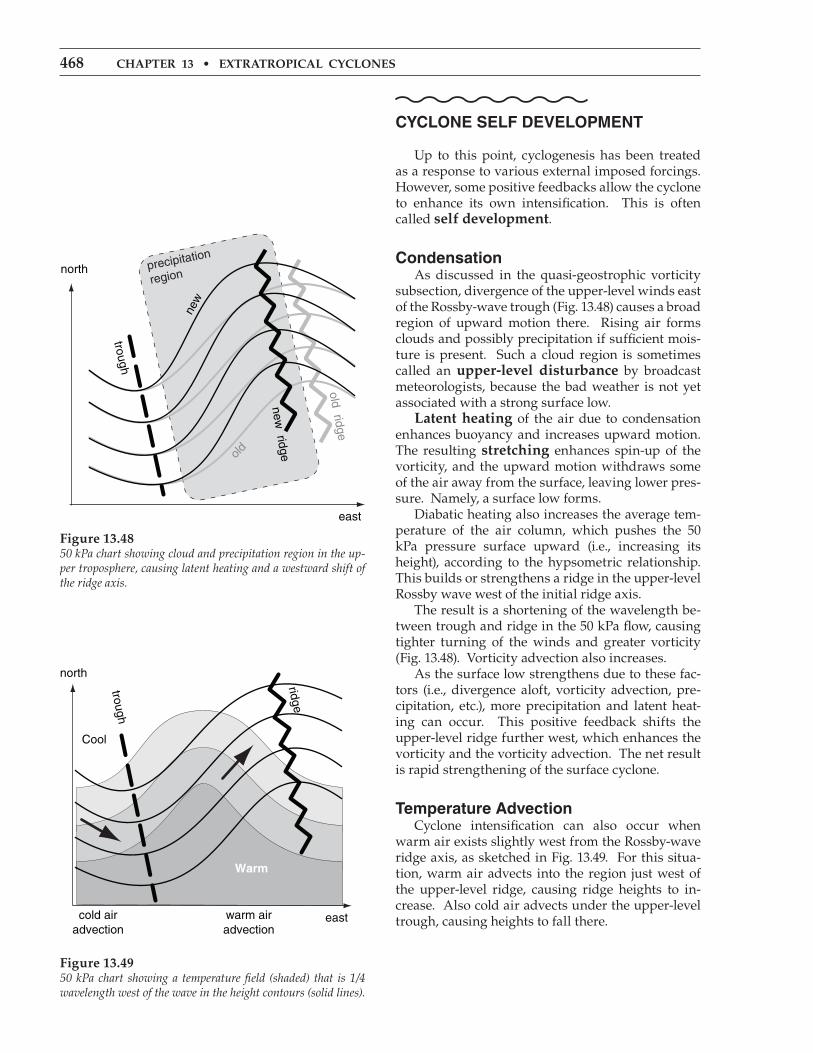
468 chaptEr 13 • Extratropical cyclonEs
CyClone selF develoPMent
Up to this point, cyclogenesis has been treated as a response to various external imposed forcings. However, some positive feedbacks allow the cyclone to enhance its own intensification. This is often called self development.
Condensation As discussed in the quasi-geostrophic vorticity subsection, divergence of the upper-level winds east of the Rossby-wave trough (Fig. 13.48) causes a broad region of upward motion there. Rising air forms clouds and possibly precipitation if sufficient mois-ture is present. Such a cloud region is sometimes called an upper-level disturbance by broadcast meteorologists, because the bad weather is not yet associated with a strong surface low. latent heating of the air due to condensation enhances buoyancy and increases upward motion. The resulting stretching enhances spin-up of the vorticity, and the upward motion withdraws some of the air away from the surface, leaving lower pres-sure. Namely, a surface low forms. Diabatic heating also increases the average tem-perature of the air column, which pushes the 50 kPa pressure surface upward (i.e., increasing its height), according to the hypsometric relationship. This builds or strengthens a ridge in the upper-level Rossby wave west of the initial ridge axis. The result is a shortening of the wavelength be-tween trough and ridge in the 50 kPa flow, causing tighter turning of the winds and greater vorticity (Fig. 13.48). Vorticity advection also increases. As the surface low strengthens due to these fac-tors (i.e., divergence aloft, vorticity advection, pre-cipitation, etc.), more precipitation and latent heat-ing can occur. This positive feedback shifts the upper-level ridge further west, which enhances the vorticity and the vorticity advection. The net result is rapid strengthening of the surface cyclone.
temperature advection Cyclone intensification can also occur when warm air exists slightly west from the Rossby-wave ridge axis, as sketched in Fig. 13.49. For this situa-tion, warm air advects into the region just west of the upper-level ridge, causing ridge heights to in-crease. Also cold air advects under the upper-level trough, causing heights to fall there.
Figure 13.4850 kPa chart showing cloud and precipitation region in the up-per troposphere, causing latent heating and a westward shift of the ridge axis.
Figure 13.4950 kPa chart showing a temperature field (shaded) that is 1/4 wavelength west of the wave in the height contours (solid lines).
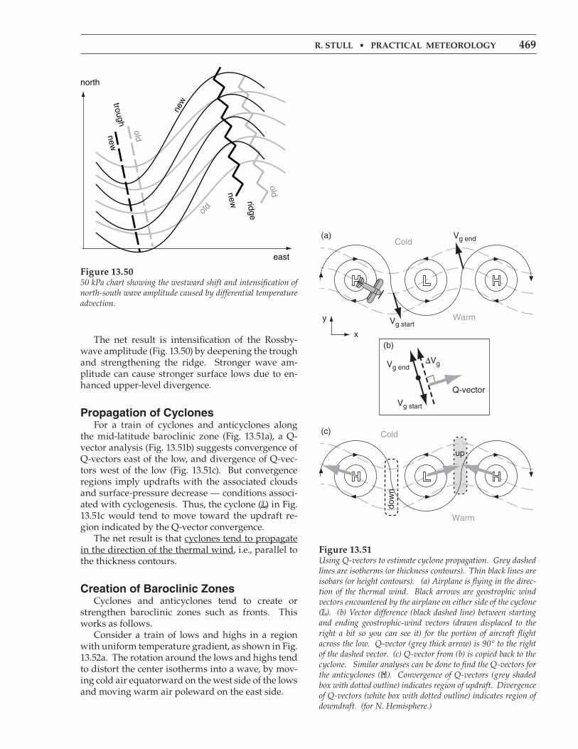
r. stull • practical MEtEorology 469
The net result is intensification of the Rossby-wave amplitude (Fig. 13.50) by deepening the trough and strengthening the ridge. Stronger wave am-plitude can cause stronger surface lows due to en-hanced upper-level divergence.
Propagation of Cyclones For a train of cyclones and anticyclones along the mid-latitude baroclinic zone (Fig. 13.51a), a Q-vector analysis (Fig. 13.51b) suggests convergence of Q-vectors east of the low, and divergence of Q-vec-tors west of the low (Fig. 13.51c). But convergence regions imply updrafts with the associated clouds and surface-pressure decrease — conditions associ-ated with cyclogenesis. Thus, the cyclone (L) in Fig. 13.51c would tend to move toward the updraft re-gion indicated by the Q-vector convergence. The net result is that cyclones tend to propagate in the direction of the thermal wind, i.e., parallel to the thickness contours.
Creation of Baroclinic Zones Cyclones and anticyclones tend to create or strengthen baroclinic zones such as fronts. This works as follows. Consider a train of lows and highs in a region with uniform temperature gradient, as shown in Fig. 13.52a. The rotation around the lows and highs tend to distort the center isotherms into a wave, by mov-ing cold air equatorward on the west side of the lows and moving warm air poleward on the east side.
Figure 13.51Using Q-vectors to estimate cyclone propagation. Grey dashed lines are isotherms (or thickness contours). Thin black lines are isobars (or height contours). (a) Airplane is flying in the direc-tion of the thermal wind. Black arrows are geostrophic wind vectors encountered by the airplane on either side of the cyclone (L). (b) Vector difference (black dashed line) between starting and ending geostrophic-wind vectors (drawn displaced to the right a bit so you can see it) for the portion of aircraft flight across the low. Q-vector (grey thick arrow) is 90° to the right of the dashed vector. (c) Q-vector from (b) is copied back to the cyclone. Similar analyses can be done to find the Q-vectors for the anticyclones (H). Convergence of Q-vectors (grey shaded box with dotted outline) indicates region of updraft. Divergence of Q-vectors (white box with dotted outline) indicates region of downdraft. (for N. Hemisphere.)
Figure 13.5050 kPa chart showing the westward shift and intensification of north-south wave amplitude caused by differential temperature advection.
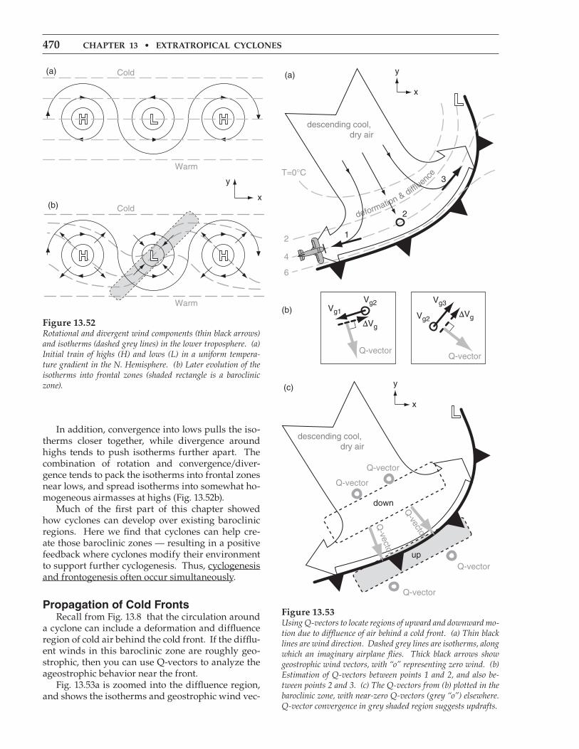
470 chaptEr 13 • Extratropical cyclonEs
In addition, convergence into lows pulls the iso-therms closer together, while divergence around highs tends to push isotherms further apart. The combination of rotation and convergence/diver-gence tends to pack the isotherms into frontal zones near lows, and spread isotherms into somewhat ho-mogeneous airmasses at highs (Fig. 13.52b). Much of the first part of this chapter showed how cyclones can develop over existing baroclinic regions. Here we find that cyclones can help cre-ate those baroclinic zones — resulting in a positive feedback where cyclones modify their environment to support further cyclogenesis. Thus, cyclogenesis and frontogenesis often occur simultaneously.
Propagation of Cold Fronts Recall from Fig. 13.8 that the circulation around a cyclone can include a deformation and diffluence region of cold air behind the cold front. If the difflu-ent winds in this baroclinic zone are roughly geo-strophic, then you can use Q-vectors to analyze the ageostrophic behavior near the front. Fig. 13.53a is zoomed into the diffluence region, and shows the isotherms and geostrophic wind vec-
Figure 13.52Rotational and divergent wind components (thin black arrows) and isotherms (dashed grey lines) in the lower troposphere. (a) Initial train of highs (H) and lows (L) in a uniform tempera-ture gradient in the N. Hemisphere. (b) Later evolution of the isotherms into frontal zones (shaded rectangle is a baroclinic zone).
Figure 13.53Using Q-vectors to locate regions of upward and downward mo-tion due to diffluence of air behind a cold front. (a) Thin black lines are wind direction. Dashed grey lines are isotherms, along which an imaginary airplane flies. Thick black arrows show geostrophic wind vectors, with “o” representing zero wind. (b) Estimation of Q-vectors between points 1 and 2, and also be-tween points 2 and 3. (c) The Q-vectors from (b) plotted in the baroclinic zone, with near-zero Q-vectors (grey “o”) elsewhere. Q-vector convergence in grey shaded region suggests updrafts.
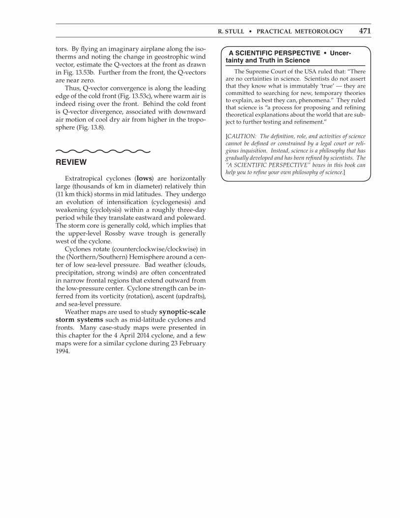
r. stull • practical MEtEorology 471
tors. By flying an imaginary airplane along the iso-therms and noting the change in geostrophic wind vector, estimate the Q-vectors at the front as drawn in Fig. 13.53b. Further from the front, the Q-vectors are near zero. Thus, Q-vector convergence is along the leading edge of the cold front (Fig. 13.53c), where warm air is indeed rising over the front. Behind the cold front is Q-vector divergence, associated with downward air motion of cool dry air from higher in the tropo-sphere (Fig. 13.8).
revieW
Extratropical cyclones (lows) are horizontally large (thousands of km in diameter) relatively thin (11 km thick) storms in mid latitudes. They undergo an evolution of intensification (cyclogenesis) and weakening (cyclolysis) within a roughly three-day period while they translate eastward and poleward. The storm core is generally cold, which implies that the upper-level Rossby wave trough is generally west of the cyclone. Cyclones rotate (counterclockwise/clockwise) in the (Northern/Southern) Hemisphere around a cen-ter of low sea-level pressure. Bad weather (clouds, precipitation, strong winds) are often concentrated in narrow frontal regions that extend outward from the low-pressure center. Cyclone strength can be in-ferred from its vorticity (rotation), ascent (updrafts), and sea-level pressure. Weather maps are used to study synoptic-scale storm systems such as mid-latitude cyclones and fronts. Many case-study maps were presented in this chapter for the 4 April 2014 cyclone, and a few maps were for a similar cyclone during 23 February 1994.
a sCientiFiC PersPeCtive • uncer-tainty and truth in science
The Supreme Court of the USA ruled that: “There are no certainties in science. Scientists do not assert that they know what is immutably ‘true’ — they are committed to searching for new, temporary theories to explain, as best they can, phenomena.” They ruled that science is “a process for proposing and refining theoretical explanations about the world that are sub-ject to further testing and refinement.”
[CAUTION: The definition, role, and activities of science cannot be defined or constrained by a legal court or reli-gious inquisition. Instead, science is a philosophy that has gradually developed and has been refined by scientists. The “A SCIENTIFIC PERSPECTIVE” boxes in this book can help you to refine your own philosophy of science.]
472 chaptEr 13 • Extratropical cyclonEs
inFo • landfalling Pacific Cyclones
Mid-latitude cyclones that form over the warm ocean waters east of Japan often intensify while ap-proaching the dateline (180° longitude). But by the time they reach the eastern North Pacific ocean they are often entering the cyclolysis phase of their evolu-tion. Thus, most landfalling cyclones that reach the Pacific Northwest coast of N. America are already oc-cluded and are spinning down. The cyclone labeled L1 in Fig. 13.54 has just started to occlude. Satellite images of these systems show a characteristic tilted-“T” ( T ) shaped cloud structure (grey shaded in Fig. 13.54), with the cold front, occlud-ed front, and a short stub of a warm front. As the cyclone translates further eastward, its translation speed often slows and the low center turns northward toward the cold waters in the Gulf of Alaska — a cyclone graveyard where lows go to die. In the late occluded phase, satellite images show a characteristic “cinnamon roll” cloud structure, such as sketched with grey shading for cyclone L2. For cyclone L2, when the cold front progresses over the complex mountainous terrain of the Pacific Northwest (British Columbia, Washington, Oregon), the front becomes much more disorganized and dif-ficult to recognize in satellite and surface weather observations (as indicated with the dashed line over British Columbia). The remaining portion of L2’s cold front still over the Pacific often continues to progress toward the southeast as a “headless” front (seemingly detached from its parent cyclone L2).
Figure 13.54Sketch of occluding mid-latitude cyclones approaching the Pacific Northwest coast of N. America. (continues in next column)
inFo • Pacific Cyclones (continued)
Sometimes there is a strong “pre-frontal jet” of fast low-altitude winds just ahead of the cold front, as shown by the black arrows in Fig. 13.54. If the source region of this jet is in the humid sub-tropi-cal air, then copious amounts of moisture can be advected toward the coast by this atmospheric riv-er. If the source of this jet is near Hawaii, then the conveyor belt of moist air streaming toward N. Amer-ica is nicknamed the “pineapple Express”. When this humid air hits the coast, the air is forced to rise over the mountains. As the rising air cools adiabatically, clouds and orographic precipita-tion form over the mountains (indicated by “m” in Fig. 13.54). Sometimes the cold front stalls (stops ad-vancing) while the pre-frontal jet continues to pump moisture toward the mountains. This atmospheric-river situation causes extremely heavy precipitation and flooding. Fig. 13.55 shows an expanded view of the Van-couver, Seattle, Victoria region (corresponding to the lower-right “m” from Fig. 13.54). Low-altitude winds split around the Olympic Mountains, only to con-verge (thick dashed line) in a region of heavy rain or snow called the olympic Mountain convergence Zone (also known as the puget sound conver-gence Zone in the USA). The windward slopes of mountain ranges often receive heavy orographic pre-cipitation (dotted ovals), while in between is often a rain shadow of clearer skies and less precipitation.
Figure 13.55Zoomed view of the Pacific Northwest. Pacific Ocean, sounds, and straits are white, while higher terrain is shaded darker. Arrows represent low-altitude wind.
r. stull • practical MEtEorology 473
hoMeWork exerCises
Broaden knowledge & ComprehensionFor all the exercises in this section, collect informa-tion from the internet. Don’t forget to cite the web site URLs that you use.
B1. Collect weather maps for a new case-study cy-clone assigned by your instructor. Use these maps to explain the processes involved in the evolution of this cyclone.
B2. What are some web sites that provide data on damage, deaths, and travel disruptions due to storms?
B3. Same as exercise B1, but use the maps to create a sketch of the 3-D nature of the storm, and how the storm dynamics affect its evolution.
B4. Find weather maps of common cyclogenesis lo-cations and storm tracks.
B5. Get weather maps that display how a cyclone is affected as it moves over large mountain ranges, such as the North American Coast Range, Rocky Mountains, Cascade Mountains, or other significant range in the world (as assigned by your instructor).
B6. Draw on a map the path of a cyclone center, and encircle regions on that map experiencing bad weather (heavy rains, blizzards, windstorms, etc.).
B7. Get maps showing cyclone bombs, and discuss their life cycle.
B8. Get upper-air weather maps (such as at 30 or 20 kPa) showing wind isotachs or geopotential height contours. Use these maps to identify Rossby wave lengths and amplitudes.
B9. Using the maps from exercise B8, measure the radius-of-curvature of troughs, and combine with wind-speed information to calculate vorticity.
B10. Get geopotential height and temperature maps for the 70 or 85 kPa isobaric surfaces. Use the meth-od of crossing isopleths to identify which point on the map has the largest temperature advection.
B11. Get geopotential height and vorticity maps on the 50 kPa isobaric surface. Identify points on the map that have the largest positive vorticity advection
and largest negative vorticity advection. Identify a location that supports cyclogenesis.
B12. Get upper-air maps of vorticity on the 70 kPa isobaric surface, and a map of 100 to 50 kPa thick-ness. For a location near a cyclone, estimate the ther-mal wind. Next, identify a point on the map having largest advection of vorticity by that thermal wind. Recall that ascent and cyclogenesis is supported at those max advection locations, as described by the omega equation.
B13. Get an upper-air map that shows contours of the height or pressure of a surface of constant poten-tial temperature (i.e., an isentropic surface). Depend-ing on the potential temperature you pick, indicate which part of the isentropic surface might be in the stratosphere (if any). Given typical wind directions (from other maps or information), indicate if the air is like ascending or descending along the isentropic surface.
B14. Get a map of isotachs for the 20 or 30 kPa iso-baric surface. Label the quadrants of relative to the jet-streak axis. Suggest locations where cyclogenesis is favored. At one of those regions, calculate verti-cal velocity in the mid-troposphere that would be caused by divergence in the jet-streak winds.
B15. Get a map of geopotential height on an iso-baric surface of 20 or 30 kPa. Comment on how the packing of heights changes as the jet stream flows in troughs and ridges.
B16. Capture a radar reflectivity image (perhaps a composite from many radars) that show the dis-tribution of dBZ around an extratropical cyclone. Comment on the amount of sea-level pressure ten-dency due to latent-heating in different parts of the cyclone.
B17. The case-study in this textbook showed weather maps of typical variables and fields often employed by meteorologists. Get and comment on the value of weather maps of other types of fields or variables, as you can acquire from national weather services or weather research centers.
B18. Find a web site that produces maps of Q-vec-tors or Q-vector divergence. Print this map and a normal surface weather map with fronts, and dis-cuss how you would anticipate the cyclone to evolve based on a Q-vector analysis.
474 chaptEr 13 • Extratropical cyclonEs
“C” in Fig. 13.20 given an average wind speed (m s–1) of: a. 20 b. 25 c. 30 d. 35 e. 40 f. 45 g. 50 h. 55 i. 60 j. 65 k. 70 l. 75 m. 80 n. 85
A8. Regarding equatorward propagation of cy-clones on the eastern slope of mountains, if a cyclone of radius 1000 km and potential vorticity of 3x10⁻⁸ m–1s–1 is over a slope as given below (∆z/∆x), find the change in relative vorticity (s–1) between the north and south sides of the cyclone. a. 1/500 b. 1/750 c. 1/1000 d. 1/1250 e. 1/1500 f. 1/1750 g. 1/2000 h. 1/2250 i. 1/2500 j. 1/2750 k. 1/3000 l. 1/3250
A9. Recall from the Atmospheric Forces and Winds chapter that incompressible mass continuity implies that ∆W/∆z = –D, where D is horizontal divergence. Find the Coriolis contribution to the stretching term (s–2) in the relative-vorticity tendency equation, giv-en the average 85 kPa divergence in Fig. 13.26 for the following USA state: a. AZ b. WI c. KS d. KY e. VA f. CO g. KA h. AB i. MD j. ID k. central TX l. NY m. IN
A10. Find the spin-up rate (s–2) of quasi-geostrophic vorticity, assuming that the following is the only non-zero characteristic: a. Geostrophic wind of 30 m s–1 from north with-in region where geostrophic vorticity increases to-ward the north by 6x10⁻⁵ s–1 over 500 km distance. b. Geostrophic wind of 50 m s–1 from west with-in region where geostrophic vorticity increases to-ward the east by 8x10⁻⁵ s–1 over 1000 km distance. c. A location at 40°N with geostrophic wind from the north of 25 m s–1. d. A location at 50°N with geostrophic wind from the south of 45 m s–1. e. A location at 35°N with vertical velocity increas-ing 0.5 m s–1 with each 1 km increase in height. f. A location at 55°N with vertical velocity decreas-ing 0.2 m s–1 with each 2 km increase in height.
A11. Find the value of geostrophic vorticity (s–1), given the following changes of (Ug, Vg) in m s–1 with 500 km distance toward the (north, east): a. (0, 5) b. (0, 10) c. (0, –8) d. (0, –20) e. (7, 0) f. (15, 0) g. (–12, 0) h. (-25, 0) i. (5, 10) j. (20, 10) k. (–10, 15) l. (–15, –12)
A12. Find the value of geostrophic vorticity (s–1), given a geostrophic wind speed of 35 m s–1 with the following radius of curvature (km). Assume the air rotates similar to a solid-body. a. 450 b. –580 c. 690 d. –750 e. 825 f. –988 g. 1300 h. –1400 i. 2430 j. –2643 k. 2810 l. –2900 m. 3014 n. –3333
applyA1. For latitude 50°N, find the approximate wave-length (km) of upper-atmosphere (Rossby) waves triggered by mountains, given an average wind speed (m s–1) of: a. 20 b. 25 c. 30 d. 35 e. 40 f. 45 g. 50 h. 55 i. 60 j. 65 k. 70 l. 75 m. 80 n. 85
A2. Find the rate of increase of the β parameter (i.e., the rate of change of Coriolis parameter with dis-tance north) in units of m–1s–1 at the following lati-tude (°N): a. 40 b. 45 c. 50 d. 55 e. 60 f. 65 g. 70 h. 80 i. 35 j. 30 k. 25 l. 20 m. 15 n. 10
A3. Given a tropospheric depth of 12 km at latitude 45°N, what is the meridional (north-south) ampli-tude (km) of upper-atmosphere (Rossby) waves trig-gered by mountains, given an average mountain-range height (km) of: a. 0.4 b. 0.6 c. 0.8 d. 1.0 e. 1.2 f. 1.4 g. 1.6 h. 1.8 i. 2.0 j. 2.2 k. 2.4 l. 2.6 m. 2.8 n. 3.0
A4. How good is the approximation of eq. (13.4) to eq. (13.3) at the following latitude (°N)? a. 40 b. 45 c. 50 d. 55 e. 60 f. 65 g. 70 h. 80 i. 35 j. 30 k. 25 l. 20 m. 15 n. 10
A5. For a troposphere of depth 12 km at latitude 43°N, find the potential vorticity in units of m–1s–1, given the following: [wind speed (m s–1) , radius of curvature (km)] a. 50 , 500 b. 50 , 1000 c. 50 , 1500 d. 50 , 2000 e. 50 , –500 f. 50 , – 1000 g. 50 , –1500 h. 50 , -2000 i. 75 , 500 j. 75 , 1000 k. 75 , 1500 l. 75 , 2000 m. 75 , –1000 n. 75 , – 2000
A6. For air at 55°N with initially no curvature, find the potential vorticity in units of m–1s–1 for a tropo-sphere of depth (km): a. 7.0 b. 7.5 c. 8.0 d. 8.5 e. 9.0 f. 9.5 g. 10.0 h. 10.5 i. 11 j. 11.5 k. 12 l. 12.5 m. 13 n. 13.5
A7. When air at latitude 60°N flows over a mountain range of height 2 km within a troposphere of depth 12 km, find the radius of curvature (km) at location
r. stull • practical MEtEorology 475
A13. What is the value of omega (Pa s–1) following a vertically-moving air parcel, if during 1 minute its pressure change (kPa) is: a. –2 b. –4 c. –6 d. –8 e. –10 f. –12 g. –14 h. –16 i. –18 j. –20 k. 0.00005 l. 0.0004 m. 0.003 n. 0.02
A14. At an altitude where the ambient pressure is 85 kPa, convert the following vertical velocities (m s–1) into omega (Pa s–1): a. 2 b. 5 c. 10 d. 20 e. 30 f. 40 g. 50 h. –0.2 i. –0.5 j. –1.0 k. –3 l. –5 m. – 0.03
A15. Using Fig. 13.15, find the most extreme value horizontal divergence (10–5 s–1) at 20 kPa over the following USA state: a. MI b. WI c. IL d. IN e. TN f. GA g. MS h. AB i. KY j. PA k. NY l. SC
A16. Find the vertical velocity (m s–1) at altitude 9 km in an 11 km thick troposphere, if the divergence (10–5 s–1) given below occurs within a 2 km thick layer within the top of the troposphere. a. 0.2 b. 1 c. 1.5 d. 2 e. 3 f. 4 g. 5 h. 6 i. –0.3 j.–0.7 k. –1.8 l. –2.2 m. –3.5 n. –5
A17. Jet-stream inflow is 30 m s–1 in a 4 km thick lay-er near the top of the troposphere. Jet-stream out-flow (m s–1) given below occurs 800 km downwind within the same layer. Find the vertical velocity (m s–1) at the bottom of that layer a. 35 b. 40 c. 45 d. 50 e. 55 f. 60 g. 65 h. 70 i. 30 j. 25 k. 20 l. 15 m. 10 n. 5
A18. Find the diagonal distance (km) from trough to crest in a jet stream for a wave of 750 km amplitude with wavelength (km) of: a. 1000 b. 1300 c. 1600 d. 2000 e. 2200 f. 2500 g. 2700 h. 3000 i. 3100 j. 3300 k. 3800 l. 4100 m. 4200 n. 4500
A19. Given the data from the previous exercise, find the radius (km) of curvature near the crests of a si-nusoidal wave in the jet stream.
A20. Find the gradient-wind speed difference (m s–1) between the jet-stream speed moving through the anticyclonic crest of a Rossby wave in the N. Hemi-sphere and the jet-stream speed moving through the trough. Use data from the previous 2 exercises, and assume a geostrophic wind speed of 75 m s–1 for a wave centered on latitude 40°N.
A21. Given the data from the previous 3 exercises. Assuming that the gradient-wind speed difference
calculated in the previous exercise is valid over a layer between altitudes 8 km and 12 km, where the tropopause is at 12 km, find the vertical velocity (m s–1) at 8 km altitude.
A22. Suppose that a west wind enters a region at the first speed (m s–1) given below, and leaves 500 km downwind at the second speed (m s–1). Find the north-south component of ageostrophic wind (m s–1) in this region. Location is 55°N. a. (40, 50) b. (30, 60) c. (80, 40) d. (70, 50) e. (40, 80) f. (60, 30) g. (50, 40) h. (70, 30) i. (30, 80) j. (40, 70) k. (30, 70) l. (60, 20)
A23. Use the ageostrophic right-hand rule to find the ageostrophic wind direction for the data of the previous problem.
A24. Using the data from A22, find the updraft speed (m s–1) into a 4 km thick layer at the top of the troposphere, assuming the half-width of the jet streak is 200 km.
A25. Suppose that the thickness of the 100 - 50 kPa layer is 5.5 km and the Coriolis parameter is 10–4 s–1. A 20 m s–1 thermal wind from the west blows across a domain of x dimension given below in km. Across that domain in the x-direction is a decrease of cy-clonic relative vorticity of 3x10⁻⁴ s–1. What is the value of mid-tropospheric ascent velocity (m s–1), based on the omega equation? a. 200 b. 300 c. 400 d. 500 e. 600 f. 700 g. 800 h. 900 i. 1000 j. 1100 k. 1200 l. 1300 m. 1400 n. 1400
A26. On the 70 kPa isobaric surface, ∆Ug/∆x = (4 m s–1)/(500 km) and ∆T/∆x = ___°C/(500 km), where the temperature change is given below. All other gradi-ents are zero. Find the Q-vector components Qx, Qy, and the magnitude and direction of Q. a. 1 b. 1.5 c. 2 d. 2.5 e. 3 f. 3.5 g. 4 h. 4.5 i. 5 j. 5.5 k. 6 l. 6.5 m. 7 n. 7.5
A27. Find Q-vector magnitude on the 85 kPa isobaric surface if the magnitude of the horizontal tempera-ture gradient is 5°C/200 km, and the magnitude of the geostrophic-wind difference-vector component (m s–1) along an isotherm is __ /200 km, where __ is: a. 1 b. 1.5 c. 2 d. 2.5 e. 3 f. 3.5 g. 4 h. 4.5 i. 5 j. 5.5 k. 6 l. 6.5 m. 7 n. 7.5
A28. Find the mass of air over 1 m2 of the Earth’s surface if the surface pressure (kPa) is: a. 103 b. 102 c. 101 d. 99 e. 98 f. 97 g. 96 h. 95 i. 93 j. 90 k. 85 l. 80 m. 75 n. 708
476 chaptEr 13 • Extratropical cyclonEs
E8. Why are there no extratropical cyclone tracks from east to west in Fig. 13.5?
E9. Contrast the climatology of cyclone formation and tracks in the Northern vs. Southern Hemisphere (using the info in Fig. 13.5), and explain why there is a difference in behaviors based on the dynamical principles in the last half of the chapter.
E10. Justify why the tank illustration in Fig. 13.6 is a good analogy to atmospheric flow between cyclones and anticyclones.
E11. Fig. 13.7 shows the axis of low pressure tilting westward with increasing height. Explain why this tilt is expected. (Hints: On which side of the cy-clone do you expect the warm air and the cold air? The hypsometric equation in Chapter 1 tells us how fast pressure decreases with height in air of differ-ent temperatures.)
E12. Redraw Fig. 13.7 a & b for the Southern Hemi-sphere, by extending your knowledge of how cy-clones work in the Northern Hemisphere.
E13. Regarding stacking and tilting of low pressure with altitude, make a photocopy of Fig. 13.3, and on this copy for Figs. b and e draw the likely position of the trough axis near the top of the troposphere. Justify your hypothesis.
E14. Fig. 13.8 shows a warm-air conveyor bring air from the tropics. Assuming this air has high hu-midity, explain how this conveyor helps to strength-en the cyclone. Using dynamical principles from the last half of the chapter to support your explanation.
E15. Fig. 13.10a has coarse temporal resolution when it shows the evolution of the case-study cyclone. Based on your knowledge of cyclone evolution, draw two weather maps similar to Fig. 13.10a, but for 12 UTC 3 Apr 2014 and 00 UTC 4 Apr 2014.
E16. Speculate on why the hail reports in Fig. 13.9 are mostly in different regions than the wind-dam-age reports.
E17. From the set of case-study maps in Figs. 13.9 through 13.19, if you had to pick 3 maps to give you the best 5-D mental picture of the cyclones, which 3 would you pick? Justify your answer.
E18. Of the following isosurfaces (height, pressure, thickness, and potential temperature), which one seems the most peculiar (unusual, illogical) to you?
A29. Assume the Earth’s surface is at sea level. Find the vertical velocity (m s–1) at height 3 km above ground if the change of surface pressure (kPa) dur-ing 1 hour is: a. –0.5 b. –0.4 c. –0.3 d. –0.2 e. –0.1 f. 0.1 g. 0.2 h. 0.4 i. 0.6 j. 0.8 k. 1.0 l. 1.2 m. 1.4
A30. Given the rainfall (mm) accumulated over a day. If the condensation that caused this precipita-tion occurred within a cloud layer of thickness 6 km, then find the virtual-temperature warming rate (°C day–1) of that layer due to latent heat release. a. 1 b. 50 c. 2 d. 45 e. 4 f. 40 g. 5 h. 35 i. 7 j. 30 k. 10 l. 25 m. 15 n. 20
A31. For the data in the previous exercise, find the rate of decrease of surface pressure (kPa) per hour, assuming an average air temperature of 5°C.
evaluate & analyzeE1. Compare the similarities and differences be-tween cyclone structure in the Northern and South-ern Hemisphere?
E2. In the Cyclogenesis & Cyclolysis section is a list of conditions that favor rapid cyclogenesis. For any 3 of those bullets, explain why they are valid based on the dynamical processes that were described in the last half of the chapter.
E3. For a cyclone bomb, are the winds associated with that cyclone in geostrophic equilibrium? Hints: consider the rate of air-parcel acceleration, based on Newton’s 2nd Law. Namely, can winds accelerate fast enough to keep up with the rapidly increasing pressure gradient?
E4. Make a photocopy of Fig. 13.3. For each one of the figure panels on this copy, infer the centerline position of the jet stream and draw it on those dia-grams.
E5. Create a 6-panel figure similar to Fig. 13.3, but for cyclone evolution in the Southern Hemisphere.
E6. Justify the comment that cyclone evolution obeys Le Chatelier’s Principle.
E7. Refer back to the figure in the General Circu-lation chapter that sketches the position of moun-tain ranges in the world. Use that information to hypothesize favored locations for lee cyclogenesis in the world, and test your hypothesis against the data in Fig. 13.5.
r. stull • practical MEtEorology 477
What questions would you want to ask to help you learn more about that one isosurface?
E19. Starting with a photocopy of the 4 height charts in the left column of Figs. 13.13, use a different color pen/pencil for each isobaric surface, and trace all the height contours onto the same chart. Analyze the tilt with height of the axis of low pressure, and explain why such tilt does or does not agree with the state of cyclone evolution at that time.
E20. Compare and contrast the 85 kPa temperature map of Fig. 13.14 with the thickness map of Fig. 13.16 for the case-study storm. Why or why not would you expect them to be similar?
E21. Compare the wind vectors of Fig. 13.13 with the heights in Fig. 13.13. Use your understanding of wind dynamics to explain the relationship between the two maps.
E22. In the vertical cross section of Fig. 13.19a, why are the isentropes packed more closely together in the stratosphere than in the troposphere? Also, why is the tropopause higher on the right side of that figure? [Hints: Consider the standard atmosphere temperature profile from Chapter 1. Consider the General Circulation chapter.]
E23. Describe the relationship between the surface values of isentropes in Fig. 13.19a and the tempera-ture values along cross-section A - A’ in Fig. 13.14 (bottom left).
E24. In Fig. 13.20, how would lee cyclogenesis be af-fected if the tropopause perfectly following the ter-rain elevation? Explain.
E25. In Fig. 13.20, speculate on why the particular set of Rossby waves discussed in that section are known as “stationary” waves.
E26. Can “stationary” Rossby waves such as in Fig. 13.20 occur near the equator? If so, what are their characteristics?
E27. Given zonal flow of the whole troposphere (12 km depth) hitting a semi-infinite plateau at 32°N latitude. Use math to explain the flow behavior over the plateau, assuming a 2 km plateau height above sea level. Assume the tropopause height doesn’t change. Would the triggering of cyclones, and the wavelength of planetary waves be different? Why? Can you relate your answer to weather over the Ti-betan Plateau?
E28. Considering the terrain height changes, would anticyclones be triggered upwind of mountain rang-es, analogous to lee-side cyclogenesis? Justify your answer, and discuss how you can confirm if this happens in the real atmosphere.
E29. Suppose that all of North America is nearly at sea level, except for a 2 km deep valley that is 500 km wide, running north-south across the center of North America (assume the valley is not filled with water). Explain what Rossby waves would be trig-gered, and the associated weather downwind.
E30. Summer tropopause height is higher, and jet-stream winds are slower, than in winter. Explain the seasonal differences you would expect in ter-rain-triggered Rossby waves, if any.
E31. If extratropical cyclones tend to propagate equatorward on the lee side of mountain ranges, is there any geographic feature that would cause these storms to propagate poleward? Justify.
E32. Fig. 13.22 highlights 3 important attributes of cyclones that are discussed in greater detail in the last half of the chapter. Speculate on why we study these attributes separately, even though the caption to that figure discusses how all 3 attributes are re-lated.
E33. For cyclogenesis we focused on three attributes: vertical velocity, vorticity, and pressure-tendency at sea level. What attributes would you want to focus on to anticipate cyclolysis? Explain.
E34. Three vorticity tilting terms are given in eq. (13.9), but just the first tilting term was illustrated in Fig. 13.23d. Draw figures for the other two terms.
E35. Except for the last term in the full vorticity ten-dency equation, all the other terms can evaluate to be positive or negative (i.e., gain or loss of relative vorticity). What is it about the mathematics of the turbulent drag term in that equation that always make it a loss of relative vorticity?
E36. Based on what you learned from Fig. 13.24, what tips would you teach to others to help them easily find regions of PVA and NVA.
E37. Make a diagram that shows vertical advection of vorticity, similar to the drawing in Fig. 13.23a.
E38. If drag were the only non-zero term on the right side of eq. (13.9), then how would vorticity change
478 chaptEr 13 • Extratropical cyclonEs
E50. Consider a steady, straight jet stream from west to east. Instead of a jet streak of higher wind speed imbedded in the jet stream, suppose the jet streak has lower wind speed imbedded in the jet stream. For the right and left entrance and exit regions to this “slow” jet streak, describe which ones would support cyclogenesis at the surface.
E51. Does the “Ageostrophic right-hand rule” work in the Southern Hemisphere too? Justify your an-swer based on dynamical principles.
E52. Eq. (13.25) was for a west wind, and eq. (13.26) was for a south wind. What method would you use to estimate ageostrophic wind if the wind was from the southwest?
E53. Fig. 13.34 suggests low-altitude convergence of air toward cyclones (lows), rising motion, and high-altitude divergence. Is this sketch supported by the case-study data from Figs. 13.15, 13.25, and 13.26?
E54. The green arrows showing near-surface winds are plotted in Fig. 13.34 as a component of the sec-ondary circulation. What drives these near-surface winds? (Hint: Recall that winds are driven by forc-es, according to Newton.)
E55. a. Use Figs. 12.12 from the Fronts & Airmasses chapter to find the location where horizontal tem-perature advection is greatest near a warm front. b. Similar questions but using Fig. 12.11 for cold fronts. Hint: Use the technique shown in the INFO box for max advection in Chapter 13.
E56. Discuss how Fig. 13.37 relates to the omega equation, and how the figure and equation can be used to locate regions that favor cyclogenesis.
E57. Create a new form for the omega equation, based on: a. the change of geostrophic wind with height; b. the temperature change in the horizontal.Hint: The horizontal-temperature gradient is relat-ed to the geostrophic-wind vertical gradient by the thermal-wind relationship.
E58. What steps and assumptions must you make to change eq. (13.28 into eq. (13.29)?
E59. Would the omega equation give any verti-cal motion for a situation having zero temperature gradient in the horizontal (i.e., zero baroclinicity)? Why?
with time if initially the flow had some amount of positive vorticity?
E39. Devise a tilting term for vertical vorticity that is tilted into horizontal vorticity.
E40. For what situations might the quasi-geostroph-ic approximation be useful, and for what situations would it be inappropriate?
E41. The quasi-geostrophic vorticity equation in-cludes a term related to vorticity advection by the geostrophic wind. The omega equation has a term related to vorticity advection by the thermal wind. Contrast these terms, and how they provide infor-mation about cyclogenesis.
E42. Employ Figs. 13.9 - 13.19 to estimate as many vorticity-tendency terms as reasonably possible for that case study event, on the 50 kPa isobaric surface at the location of the “X”.
E43. Create a “toy model” similar to Fig. 13.27, but focus on the vorticity effects east of the ridge axis. Use this to help explain anticyclogenesis.
E44. If nothing else changes except latitude, explain the relationship between Rossby-wave radius-of-curvature and latitude.
E45. Why does jet-stream curvature contribute to surface cyclogenesis east of the jet trough axis rather than west of the trough axis?
E46. In the Forces and Winds chapter you saw that the horizontal pressure gradient and wind speeds are weak. Does this physical constraint influence the possible strength of the jet-stream curvature ef-fect for cyclogenesis?
E47. At the “X” in Fig. 13.30, use the information plotted on that map to estimate how the jet-stream curvature and jet-streak processes influence changes to sea-level pressure and ascent speed in the middle of the troposphere.
E48. Make a photo copy of Fig. 13.18. Using the jet-stream curvature and jet-streak information that you can estimate from the height contours, draw on your copy the locations in the Northern Hemisphere where cyclogenesis is favored.
E49. For the jet-streak illustration of Fig. 13.32b, ex-plain why two of the quadrants have weaker conver-gence or divergence than the other two quadrants.
r. stull • practical MEtEorology 479
E60. What role does inertia play in the “geostrophic paradox”?
E61. Suppose that the 85 kPa geostrophic wind vec-tors are parallel to the height contours in Fig. 13.13 for the case-study storm. Use that information along with the 85 kPa isotherms in Fig. 13.14 to estimate the direction of the Q-vectors at the center of the fol-lowing USA state: a. IL b. IA c. MO d. KS e. AR
E62. Use the Q-vector approach to forecast where cyclogenesis might occur in the Pacific Northwest USA (in the upper left quadrant of Figs. 13.40 and 13.41).
E63. In Fig. 13.43 we showed have the vertical speeds of the “leaf” in the air column could be a surrogate for changes in mass and surface pressure. Discuss the pros and cons of that approach.
E64. If rainfall rate (RR) affects surface pressure, and weather-radar echo intensity (dBZ) can be used to estimate rainfall rate, then devise an equation for surface-pressure change as a function of dBZ.
E65. Considering surface-pressure tendency, what cyclogenesis information can be gained from Dop-pler velocities measured by weather radar? State the limitations of such an approach.
E66. Are there situations for which cyclolysis (quan-tified by sea-level pressure tendency) might be caused by latent heating. Justify your arguments.
E67. In Fig. 13.47, describe the dynamics that makes the time of maximum convergence in the boundary layer occur after the time of maximum divergence in the jet stream, during cyclone evolution.
E68. Suppose that the temperature wave in Fig. 13.49 was a quarter of a wavelength east of the height wave. Would the flow differ from that sketched in Fig. 13.50? Speculate on how likely it is that the tem-perature wave is shifted this way.
E69. Do you think that anticyclones could self de-velop? Explain what processes could make this hap-pen.
E70. Explain why the Q-vector analysis of Fig. 13.51 indicates the propagation of cyclones is toward the east. Also explain why this relates to self-propaga-tion rather than relating to cyclogenesis driven by the jet-stream flow.
E71. Use Fig. 13.52 to explain why fronts are associ-ated with cyclones and not anticyclones. The same figure can be used to explain why airmasses are as-sociated with anticyclones. Discuss.
E72. If global baroclinicity is absent (e.g., no air-temperature gradient between the equator and the poles), could there be cyclogenesis? Why?
E73. Explain how the up- and down-couplet of air motion in Fig. 13.53c (as diagnosed using Q-vectors), works in a way to strengthen and propagate the cold front.
E74. Use a Q-vector analysis to speculate on the dy-namics needed to cause warm fronts to strengthen and propagate.
E75. Synthesize a coherent description of the dy-namics of the case-study cyclone, based on informa-tion from the weather maps that help you estimate ascent, spin-up, and sea-level pressure tendency.
E76. Compare and contrast the Pacific cyclones of Fig. 13.54 with the case-study cyclone of Figs. 13.13 - 13.15.
synthesizeS1. Consider Fig. 13.6. What if frictional drag is zero at the bottom of the atmosphere (in the boundary layer). Describe differences in the resulting climate and weather.
S2. What if the case-study cyclone of Figs. 13.9 - 13.19 occurred in February rather than April, what broad aspects of the storm data would change, if at all?
S3. What if there were no mountain ranges oriented south-north in North America. Describe differences in the resulting climate and weather.
S4. What if all south-north mountain ranges disap-peared in North America, and were replaced by one west-east mountain range. Describe differences in the resulting climate and weather.
S5. Suppose western North America was cold, and eastern North America was warm. Describe the orientation of baroclinicity, the jet stream, and dif-ferences in resulting climate and weather relative to our actual climate and weather.
S6. Describe changes to Rossby waves and cyclo-genesis for an Earth that rotates twice as fast as the real Earth.
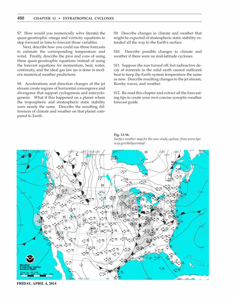
480 chaptEr 13 • Extratropical cyclonEs
S7. How would you numerically solve (iterate) the quasi-geostrophic omega and vorticity equations to step forward in time to forecast those variables. Next, describe how you could use those forecasts to estimate the corresponding temperature and wind. Finally, describe the pros and cons of using these quasi-geostrophic equations instead of using the forecast equations for momentum, heat, water, continuity, and the ideal gas law (as is done in mod-ern numerical weather prediction).
S8. Accelerations and direction changes of the jet stream create regions of horizontal convergence and divergence that support cyclogenesis and anticyclo-genesis. What if this happened on a planet where the tropospheric and stratospheric static stability were nearly the same. Describe the resulting dif-ferences of climate and weather on that planet com-pared to Earth.
S9. Describe changes in climate and weather that might be expected of stratospheric static stability ex-tended all the way to the Earth’s surface.
S10. Describe possible changes to climate and weather if there were no mid-latitude cyclones.
S11. Suppose the sun turned off, but radioactive de-cay of minerals in the solid earth caused sufficient heat to keep the Earth-system temperature the same as now. Describe resulting changes to the jet stream, Rossby waves, and weather.
S12. Re-read this chapter and extract all the forecast-ing tips to create your own concise synoptic-weather forecast guide.
FRIDAY, APRIL 4, 2014
1020
1020
1015
1010
1025
100410041008
1008
1012
1012
1012
10081004
1000
1028102810241024
997
1022
1023
1000
998
1011
1012
1021
1020
1004
1004
10201020
1023
1012 10121012 1012
1016
1016
1016
1016
1016
101610001000
1024
1016
1012
1020
996 1016
0
0
32
32
32
32
32
32
32
30
40
50
100NMTrue at 40.00N
200 300 400 500
5433
75+7
74
07
3+4
4+4
5
7
+5
53504
+4
3
75 23
3
+5
+240 73
3
772
+2755 0
53+45
44 72
772
737
42 0
4+5
33
44+24
353725
4 20330
3+5
22
44
43
5454
5447
7+4
3+3
52
5050
4
+72
2+2
52
0775 0
3
55077
+2557 72
25 5352
42 5
4432
40
4030
3327
3322
3020
54
5 520
442
45
5247
52+4
47 0540
453 0
5554 0
5250 0
03557 77052
57
57 0435 0
03257 32
5 02755
45 074+47
37
525244 044
+47
40+27
30
3527
332722
3427
2
24 203
23 205
2
3220
3
30
42
524
44+3
34 2
40 2003442
2 0
3
4237 3
3+4
223
54 07453 0
3
535 3
2
43 0
42424 0
3 0
437+45
234+32
33 5
3330 4
7
22
23
3 205+4
20
24
4230
27
32
32444
4742
4542 7
3320
2 20422
37 00735
330
3 3
333 5
3
30+4
2 202
322 2
3024
24 55
53
+324
324
320
40+5
30
330
430
4 57
4744 3
3020
32225
+222 23
25
2 02
+220
3220
3525
423 4
7444
45
4342
224
50+20
2 0
4
30
40
50
100NMTrue at 40.00N
200 300 400 500
4
2275
30
40
50
100NMTrue at 40.00N
200 300 400 500
4340 0
25 04322 0
302 0
34
222 4
25 0547 0
37 20435 0
32 0
220 0
20
34 07023 0
0
25 2354 020
4 00
2 0
2077 02
25 0
45
34 053+5
33
737
4
553 0
5
4 03
73 0
2
30
40
50
100NMTrue at 40.00N
200 300 400 50070
+3270
70
7+4
700
30
40
50
100NMTrue at 40.00N
200 300 400 500
WeatherPrediction CenterAnalyst Ryan
Fig. 13.56. Surface weather map for the case-study cyclone, from www.hpc.ncep.gov/dailywxmap/ .