Embed Size (px)
Citation preview
12th International Workshop onTermination (WST 2012)
WST 2012, February 19–23, 2012, Obergurgl, Austria
Edited by
Georg Moser
12th Inte rnat iona l Workshop on Terminat ion WST 2012
Editor
Georg Moser
Institute of Computer Science
University of Innsbruck, Austria
Published online and open access by
G. Moser, Institute of Computer Science, University of Innsbruck, Austria.
Publication date
February, 2012
License
This work is licensed under a Creative Commons Attribution-Noncommercial-No Derivative Works li-
cense: http://creativecommons.org/licenses/by-nc-nd/3.0/legalcode.
In brief, this license authorises each and everybody to share (to copy, distribute and transmit) the work
under the following conditions, without impairing or restricting the authors’ moral rights:
Attribution: The work must be attributed to its authors.
Noncommercial: The work may not be used for commercial purposes.
No derivation: It is not allowed to alter or transform this work.
The copyright is retained by the corresponding authors.
iii
Preface
This volume contains the proceedings of the 12th International Workshop on Termination (WST 2012),
to be held February 19–23, 2012 in Obergurgl, Austria. The goal of the Workshop on Termination
is to be a venue for presentation and discussion of all topics in and around termination. In this way,
the workshop tries to bridge the gaps between different communities interested and active in research
in and around termination. The 12th International Workshop on Termination in Obergurgl continues
the successful workshops held in St. Andrews (1993), La Bresse (1995), Ede (1997), Dagstuhl (1999),
Utrecht (2001), Valencia (2003), Aachen (2004), Seattle (2006), Paris (2007), Leipzig (2009), and
Edinburgh (2010).
The 12th International Workshop on Termination did welcome contributions on all aspects of termination
and complexity analysis. Contributions from the imperative, constraint, functional, and logic program-
ming communities, and papers investigating applications of complexity or termination (for example in
program transformation or theorem proving) were particularly welcome.
We did receive 18 submissions which all were accepted. Each paper was assigned two reviewers. In
addition to these 18 contributed talks, WST 2012, hosts three invited talks by Alexander Krauss, Martin
Hofmann, and Fausto Spoto.
I would like to take this opportunity to thank all those that helped to organise the current Workshop
on Termination. First of let me thank the members of the program committee who provided invaluable
assistance on the scientific end of the workshop. Moreover I’d like to thank the members of the organi-
sation committee who did their best to guarantee that the actual event will be a success. Last, but not
least, I’d like to thank our sponsors, namely the Kurt Gödel Society, and the University of Innsbruck,
without whose assistance the workshop wouldn’t haven taken place.
Innsbruck, February 17, 2012 Georg Moser
WST 2012
Conference Organisation
Program Chair
Georg Moser
Program Committee
Ugo Dal Lago, Università di Bologna
Danny De Schreye, Katholieke Universiteit Leuven
Jörg Endrullis, VU University Amsterdam
Samir Genaim, Universidad Compultense de Madrid
Nao Hirokawa, Japan Advanced Institut of Science and Technology
Georg Moser, University of Innsbruck
Albert Rubio, Universitat Politècnica de Catalunya
Peter Schneider-Kamp, University of Southern Denmark
René Thiemann, University of Innsbruck
Organisation Committee
Simon Bailey, University of Innsbruck
Stéphane Gimenez, University of Innsbruck
Martina Ingenhaeff, University of Innsbruck
Georg Moser, University of Innsbruck
Michael Schaper, University of Innsbruck

Contents
Abstracts of Invited Talks
Termination of Isabelle/HOL Functions – The Higher-Order Case
Alexander Krauss . . . . . . . . . . . . . . . . . . . . . . . . . . . . . . . . . . . . . . . . . . . . . . . . . . . . . . . . . . . . . . . . 7
Amortized resource analysis
Martin Hofmann . . . . . . . . . . . . . . . . . . . . . . . . . . . . . . . . . . . . . . . . . . . . . . . . . . . . . . . . . . . . . . . . 8
Termination analysis with Julia: What are we missing?
Fausto Spoto . . . . . . . . . . . . . . . . . . . . . . . . . . . . . . . . . . . . . . . . . . . . . . . . . . . . . . . . . . . . . . . . . . . . 9
Contributed Papers
On the Invariance of the Unitary Cost Model for Head Reduction
Beniamino Accattoli and Ugo Dal Lago . . . . . . . . . . . . . . . . . . . . . . . . . . . . . . . . . . . . . . . . . . 10
On a Correspondence between Predicative Recursion and Register Machines
Martin Avanzini, Naohi Eguchi, and Georg Moser . . . . . . . . . . . . . . . . . . . . . . . . . . . . . . . 15
Higher-Order Interpretations and Program Complexity
Patrick Baillot and Ugo Dal Lago . . . . . . . . . . . . . . . . . . . . . . . . . . . . . . . . . . . . . . . . . . . . . . . 20
Recent Developments in the Matchbox Termination Prover
Alexander Bau, Tobias Kalbitz, Maria Voigtländer, and Johannes Waldmann . . . . 25
The recursive path and polynomial ordering
Miquel Bofill, Cristina Borralleras, Enric Rodríguez-Carbonell, and Albert Rubio . 29
Proving Termination of Java Bytecode with Cyclic Data
Marc Brockschmidt, Richard Musiol, Carsten Otto, and Jürgen Giesl . . . . . . . . . . . . 34
Proving Non-Termination for Java Bytecode
Marc Brockschmidt, Thomas Ströder, Carsten Otto, and Jürgen Giesl . . . . . . . . . . . . 39
Termination Analysis via Monotonicity Constraints over the Integers and SAT Solving
Michael Codish, Igor Gonopolskiy, Amir M. Ben-Amram, Carsten Fuhs, and Jürgen
Giesl . . . . . . . . . . . . . . . . . . . . . . . . . . . . . . . . . . . . . . . . . . . . . . . . . . . . . . . . . . . . . . . . . . . . . . . . . . . . 44
Detecting Non-Looping Non-Termination
Fabian Emmes, Tim Enger, and Jürgen Giesl . . . . . . . . . . . . . . . . . . . . . . . . . . . . . . . . . . . 49
Binomial Interpretations
Bertram Felgenhauer . . . . . . . . . . . . . . . . . . . . . . . . . . . . . . . . . . . . . . . . . . . . . . . . . . . . . . . . . . . . 54
On Modularity of Termination Properties of Rewriting under Strategies
Bernhard Gramlich and Klaus Györgyfalvay . . . . . . . . . . . . . . . . . . . . . . . . . . . . . . . . . . . . . 59
Termination Graphs Revisited
Georg Moser and Michael Schaper . . . . . . . . . . . . . . . . . . . . . . . . . . . . . . . . . . . . . . . . . . . . . . . 64
Matrix Interpretations for Polynomial Derivational Complexity
Friedrich Neurauter and Aart Middeldorp . . . . . . . . . . . . . . . . . . . . . . . . . . . . . . . . . . . . . . . . 69
WST 2012: 12th International Workshop on Termination.
Editor: G. Moser
vi Contents
Encoding Induction in Correctness Proofs of Program Transformations as a Termination
Problem
Conrad Rau, David Sabel, and Manfred Schmidt-Schauß . . . . . . . . . . . . . . . . . . . . . . . . . 74
A Relative Dependency Pair Framework
Christian Sternagel and René Thiemann . . . . . . . . . . . . . . . . . . . . . . . . . . . . . . . . . . . . . . . . . 79
Automated Runtime Complexity Analysis for Prolog by Term Rewriting
Thomas Ströder, Fabian Emmes, Peter Schneider-Kamp, and Jürgen Giesl . . . . . . . 84
A Report on the Certification Problem Format
René Thiemann . . . . . . . . . . . . . . . . . . . . . . . . . . . . . . . . . . . . . . . . . . . . . . . . . . . . . . . . . . . . . . . . . 89
Automating Ordinal Interpretations
Harald Zankl, Sarah Winkler, and Aart Middeldorp . . . . . . . . . . . . . . . . . . . . . . . . . . . . . . 94
Termination of Isabelle/HOL Functions – The
Higher-Order Case
Alexander Krauss
QAware GmbH
München, Germany
Abstract of the Talk
This talk gives an overview on the structure of termination problems that arise in interactive
theorem proving based on higher-order logic, specifically Isabelle/HOL.
I will explain what it means to justify a recursive definition in HOL, and discuss the
extraction of termination proof obligations and some successful approaches to their automated
proof.
Then I will focus on the higher-order case, which is not fully automated, as it requires
some configuration by the user. I will discuss the state of the art and the issues that make
further automation difficult.
© A. Krauss;
licensed under Creative Commons License NC-ND
WST 2012: 12th International Workshop on Termination.
Editor: G. Moser; pp. 7–7
Amortized resource analysis
Martin Hofmann
Institut für Informatik
Ludwig-Maximilians-Universität München, Germany
Abstract of the Talk
Resource analysis aims at automatically determining and upper bound on the resource usage
of a program as a function of its input size. Resources in this context can be runtime, heap-
and stack size, number of occurrences of certain events, etc.
The amortized approach to resource analysis works by associating “credits” with elements
of data structures and to “pay” for each consumption of resource from the credits currently
available. In this way composite programs and programs with intermediate data structures
can be analysed more conveniently than would otherwise be the case.
Amortization was introduced by Tarjan in the 70s in the context of manual complexity
analyis of algorithms. More recently, it has been used for type-based automatic resource
analysis.
The talk surveys the key concepts with simple examples and then moves on to survey
some recent papers, notably the inference of multivariate polynomial resource bounds for
functional programs and a type-based resource analysis of Java-like object-oriented programs.
I will also try to say something about possible connections with term rewriting, in particular
polynomial interpretations.
© M. Hofmann;
licensed under Creative Commons License NC-ND
WST 2012: 12th International Workshop on Termination.
Editor: G. Moser; pp. 8–8
Termination analysis with Julia: What are we
missing?
Fausto Spoto
Dipartimento di Informatica,
Università di Verona, Italy
Abstract of the Talk
I will describe the structure and underlying theory of the termination analysis module
of the Julia static analyzer. This tool is based on abstract interpretation and translates
Java/Android code into CLP, whose termination is more easily proved. I will give some
details about the implementation and the trade-offs between precision and efficiency. I will
then present the results of analysis of a set of large programs and see concrete examples of
where the tool does not prove termination. This will give us an idea of which actual problems
are faced by a termination analyzer and how/if they can be solved in the future.
© F. Spoto;
licensed under Creative Commons License NC-ND
WST 2012: 12th International Workshop on Termination.
Editor: G. Moser; pp. 9–9
On the Invariance of the Unitary Cost Model for
Head Reduction∗
Beniamino Accattoli1 and Ugo Dal Lago2
1 INRIA & LIX (École Polytechnique)[email protected]
2 Università di Bologna & [email protected]
Abstract
The λ-calculus is a widely accepted computational model of higher-order functional programs,
yet there is not any direct and universally accepted cost model for it. As a consequence, the com-
putational difficulty of reducing λ-terms to their normal form is typically studied by reasoning on
concrete implementation algorithms. Here, we show that when head reduction is the underlying
dynamics, the unitary cost model is indeed invariant. This improves on known results, which
only deal with weak (call-by-value or call-by-name) reduction. Invariance is proved by way of
a linear calculus of explicit substitutions, which allows to nicely decompose any head reduction
step in the λ-calculus into more elementary substitution steps, thus making the combinatorics
of head-reduction easier to reason about. The technique is also a promising tool to attack what
we see as the main open problem, namely understanding for which normalizing strategies the
unitary cost model is invariant, if any.
1998 ACM Subject Classification F.4.1 - Mathematical Logic, F.4.2 - Grammars and Other
Rewriting Systems
Keywords and phrases Lambda Calculus, Invariance, Cost Models
1 Introduction
Giving an estimate of the amount of time T needed to execute a program is a natural
refinement of the termination problem, which only requires to decide whether T is either
finite or infinite. The shift from termination to complexity analysis brings more informative
outcomes at the price of an increased difficulty. In particular, complexity analysis depends
much on the chosen computational model. Is it possible to express such estimates in a way
which is independent from the specific machine the program is run on? An answer to this
question can be given following computational complexity, which classifies functions based on
the amount of time (or space) they consume when executed by any abstract device endowed
with a reasonable cost model, depending on the size of input. When can a cost model be
considered reasonable? The answer lies in the so-called invariance thesis [14]: any time cost
model is reasonable if it is polynomially related to the (standard) one of Turing machines.
If programs are expressed as rewrite systems (e.g. as first-order TRSs), an abstract but
effective way to execute programs, rewriting itself, is always available. As a consequence,
a natural time cost model turns out to be derivational complexity, namely the (maximum)
number of rewrite steps which can possibly be performed from the given term. A rewriting
step, however, may not be an atomic operation, so derivational complexity is not by definition
∗ This work was partially supported by the ARC INRIA ETERNAL project.
© B. Accattoli and U. Dal Lago;licensed under Creative Commons License NC-ND
WST 2012: 12th International Workshop on Termination.Editor: G. Moser; pp. 10–14
B. Accattoli and U. Dal Lago 11
invariant. For first-order TRSs, however, derivational complexity has been recently shown to
be an invariant cost model, by way of term graph rewriting [7, 5].
The case of λ-calculus is definitely more delicate: if β-reduction is weak, i.e., if it cannot
take place in the scope of λ-abstractions, one can see λ-calculus as a TRS and get invariance
by way of the already cited results [6], or by other means [12]. But if one needs to reduce
“under lambdas” because the final term needs to be in normal form (e.g., when performing
type checking in dependent type theories), no invariance results are known at the time of
writing.
Here we give a partial solution to this problem, by showing that the unitary cost model is
indeed invariant for the λ-calculus endowed with head reduction, in which reduction can take
place in the scope of λ-abstractions, but can only be performed in head position. Our proof
technique consists in implementing head reduction in a calculus of explicit substitutions.
Explicit substitutions were introduced to close the gap between the theory of λ-calculus
and implementations [1]. Their rewriting theory has also been studied in depth, after Melliès
showed the possibility of pathological behaviors [9]. Starting from graphical syntaxes, a new
at a distance approach to explicit substitutions has recently been proposed [4]. The new
formalisms are simpler than those of the earlier generation, and another thread of applications
— to which this paper belongs — also started: new results on λ-calculus have been proved by
means of explicit substitutions [4, 3].
Here, we make use of the linear-substitution calculus Λ[·], a slight variation over a calculus
of explicit substitutions introduced by Robin Milner [10]. The variation is inspired by the
structural λ-calculus [4]. We study in detail the relation between λ-calculus head reduction
and linear head reduction [8], the head reduction of Λ[·], and prove that the latter can
be at most quadratically longer than the former. This is proved without any termination
assumption, by a detailed rewriting analysis.
To get the Invariance Theorem, however, other ingredients are required:
1. The Subterm Property. Linear head reduction has a property not enjoyed by head β-
reduction: linear substitutions along a reduction t⊸∗ u duplicates subterms of t only. It
easily follows that ⊸-steps can be simulated by Turing machines in time polynomial in
the size of t and the length of ⊸∗.
2. Compact representations. Explicit substitutions, decomposing β-reduction into more
atomic steps, allow to take advantage of sharing and thus provide compact representations
of terms, avoiding the exponential blowups of term size happening in plain λ-calculus. Is
it reasonable to use these compact representations of λ-terms? We answer affirmatively,
by exhibiting a dynamic programming algorithm for checking equality of terms with
explicit substitutions modulo unfolding, and proving it to work in polynomial time in the
size of the involved compact representations.
3. Head simulation of Turing machines. We also provide the simulation of Turing machines
by λ-terms. We give a new encoding of Turing machines, since the known ones do not
work with head β-reduction, and prove it induces a polynomial overhead.
We emphasize the result for head β-reduction, but our technical detour also proves invariance
for linear head reduction. To our knowledge, we are the firsts to use the fine granularity of
explicit substitutions for complexity analysis. Many calculi with bounded complexity (e.g.
[13]) use let-constructs, an avatar of explicit substitutions, but they do not take advantage
of the refined dynamics, as they always use big-steps substitution rules.
Arguably, the main contribution of this paper lies in the technique rather than in the
invariance result. Indeed, the main open problem in this area, namely the invariance of the
unitary cost model for any normalizing strategy remains open. But even if linear explicit
WST 2012
12 On the Invariance of the Unitary Cost Model for Head Reduction
substitutions cannot be directly applied to the problem, the authors strongly believe that this
is anyway a promising direction, on which they are actively working at the time of writing.
2 Linear Explicit Substitutions and the Unitary Cost Model
First of all, we introduce the λ-calculus. Its terms are given by the grammar:
t, u, r ∈ Tλ :: x | Tλ Tλ | λx.Tλ
and its reduction rule →β is defined as the context closure of (λx.t) u 7→β tx/u. We will
mainly work with head reduction, instead of full β-reduction. We define head reduction as
follows. Let an head context H be defined by:
H ::= [·] | H Tλ | λx.H.
Then define head reduction →h as the closure by head contexts of 7→β . Our definition of
head reduction is slightly more liberal than the usual one, but none of its properties are lost.
The calculus of explicit substitutions we are going to use is a minor variation over a
simple calculus introduced by Milner [10]. The grammar is standard:
t, u, r ∈ T :: x | T T | λx.T | T [x/T ].
The term t[x/u] is an explicit substitution and binds x in t. Given a term t with explicit
substitutions, its unfolding is the λ-term without explicit substitutions defined as follows:
x
→
:= x
→
(t u)
→
:= t
→
u
→
(λx.t)
→
:= λx.t
→
(t[x/u])
→
:= t
→
x/u
→
.
Head contexts are defined by the following grammar:
H ::= [·] | H T | λx.H | H[x/T ].
We define head linear reduction ⊸ as ⊸dB ∪⊸ls, where ⊸dB and ⊸ls are the closure by
head contexts of:
(λx.t)L u 7→dB t[x/u]L H[x][x/u] 7→ls H[u][x/u]
The key property of linear head reduction is the Subterm Property. A term u is a box-subterm
of a term t if t has a subterm of the form r u or of the form r[x/u] for some r.
Lemma 1 (Subterm Property). If t⊸∗ u and r is a box-suterm of u, then r is a box-subterm
of t.
Linear head substitution steps duplicate sub-terms, but the Subterm Property guarantees that
only sub-terms of the initial term t are duplicated, and thus each step can be implemented
in time polynomial in the size of t, which is the size of the input, the fundamental parameter
for complexity analysis. This is in sharp contrast with what happens in the λ-calculus, where
the cost of a β-reduction step is not even polynomially related to the size of the initial term.
The subterm property does not only concern the cost of implementing reduction steps,
but also the size of intermediate terms:
Corollary 2. There is a polynomial p : N× N→ N such that if t⊸k u then |u| ≤ p(k, |t|).
From a rewriting analysis of head reduction and linear head reduction we get the
following:
B. Accattoli and U. Dal Lago 13
1. Any ⊸-reduction ρ projects via unfolding to a →h-reduction ρ
→
having as length exactly
the number of ⊸dB steps in ρ;
2. Any →h-reduction ρ can be simulated by a ⊸-reduction having as many ⊸dB-steps as
the the steps in ρ, followed by unfolding;
Moreover, by means of a simple measure and the subterm property we prove:
Theorem 3. Let t ∈ Tλ. If ρ : t ⊸n u then n = O(|ρ|2
dB), where |ρ|dB is the number of
⊸dB-steps in ρ.
From the theorem and the previous two points there is a quadratic — and thus polynomial —
relation between →h-reductions and ⊸-reduction from a given term. Therefore, we get:
Corollary 4 (Invariance, Part I). There is a polynomial time algorithm that, given t ∈ Tλ,
computes a term u such that u
→
= r if t has →h-normal form r and diverges if u has no
→h-normal form. Moreover, the algorithm works in polynomial time on the derivation
complexity of the input term.
One may now wonder why a result like Corollary 4 cannot be generalized to, e.g., leftmost-
outermost reduction, which is a normalizing strategy. Actually, linear explicit substitutions
can be endowed with a notion of reduction by levels capable of simulating the leftmost-
outermost strategy in the same sense as linear head-reduction simulates head-reduction here.
And, noticeably, the subterm property continues to hold. What is not true anymore, however,
is the quadratic bound we have proved in this section: in the leftmost-outermost strategy,
one needs to perform too many substitutions not related to any β-redex. If one wants to
generalize Corollary 4, in other words, one needs to further optimize the substitution process.
But this is outside the scope of this paper.
One may also wonder whether explicit substitutions are nothing more than a way to hide
the complexity of the problem under the carpet of compactness: what if we want to get the
normal form in the usual, explicit form? Consider the sequence of λ-terms defined as follows,
by induction on a natural number n (where u is the lambda term yxx): t0 = u and for every
n ∈ N, tn+1 = (λx.tn)u. tn has size linear in n, and tn rewrites to its normal form rn in
exactly n steps by head reduction strategy:
t0 ≡ u ≡ r0
t1 → yuu ≡ yr0yr0 ≡ r1
t2 → (λx.t0)(yuu) ≡ (λx.u)(r1)→ yr1r1 ≡ r2
...
For every n, however, rn+1 contains two copies of rn, hence the size of rn is exponential in n.
As a consequence, if we stick to the head strategy and if we insist on normal forms to be
represented explicitly, without taking advantage of the shared representation provided by
explicit substitutions, the number of head steps is not an invariant cost model: in a linear
number of steps we reach an object which cannot even be written down in polynomial time.
This phenomenon is due to the λ-calculus being a very inefficient way to represent λ-terms.
Explicit substitutions represent normal forms compactly, avoiding the exponential blow-up.
We prove that this compact representation is reasonable in the following sense: even if
computing the unfolding of a term t ∈ Λ[·] takes exponential time, comparing the unfoldings
of two terms t, u ∈ Λ[·] for equality can be done in polynomial time (details in [2]). This
way, linear explicit substitutions are proved to be a succint, acceptable, encoding of λ-terms
in the sense of Papadimitriou [11]. The algorithm which compares the unfoldings is based
WST 2012
14 On the Invariance of the Unitary Cost Model for Head Reduction
on dynamic programming: for every subterm of t (resp. u) it computes its unfolding with
respect to the substitutions in t (resp. u) and compare it with the unfoldings of the subterms
of the other term. This can be done without really computing those unfoldings (which would
require exponential space and time).
We address also the converse relation between Turing Machines and λ-calculus, by giving
a new encoding of Turing Machines into the λ-calculus (details in [2]). The transitions of
Turing Machines are simulated by head reduction in such a way that the running time of
the machine is polynomially related to the length of the head reduction of the encoding
term. The encoding is along the lines of existing representations of Turing Machines into
λ-calculus, except that 1) natural numbers are represented via Scott numerals (instead
of Church numerals), which are a better representation when evaluation is given by head
reduction, and 2) The encoding is in continuation-passing style. The following theorem
completes our invariance result:
Theorem 5 (Invariance, Part II). Let ∆ be an alphabet. If f : ∆∗ → ∆∗ is computed by
a Turing machineM in time g, then there is a term U(M,∆) such that for every u ∈ ∆∗,
U(M,∆)⌈u⌉∆∗
→nh⌈f(u)⌉∆
∗
where n = O(g(|u|) + |u|).
References
1 M. Abadi, L. Cardelli, P. L. Curien, and J. J. Levy. Explicit substitutions. Journal of
Functional Programming, 1:31–46, 1991.
2 B. Accattoli and U. Dal Lago. On the invariance of the unitary cost model for head
reduction (long version). Available at http://arxiv.org/abs/1202.1641.
3 B. Accattoli and D. Kesner. The permutative λ-calculus. To appear in the proceedings of
LPAR 2012.
4 B. Accattoli and D. Kesner. The structural λ-calculus. In Proceedings of CSL 2010, volume
6247 of LNCS, pages 381–395. Springer, 2010.
5 M. Avanzini and G. Moser. Complexity analysis by graph rewriting. In Proceedings of
FLOPS 2010, volume 6009 of LNCS, pages 257–271. Springer, 2010.
6 U. Dal Lago and S. Martini. On constructor rewrite systems and the lambda-calculus. In
Proceedings of ICALP 2009, volume 5556 of LNCS, pages 163–174. Springer, 2009.
7 U. Dal Lago and S. Martini. Derivational complexity is an invariant cost model. In Pro-
ceedings of FOPARA 2010, volume 6324 of LNCS, pages 88–101. Springer, 2010.
8 G. Mascari and M. Pedicini. Head linear reduction and pure proof net extraction. Theo-
retical Computer Science, 135(1):111–137, 1994.
9 P.-A. Melliès. Typed lambda-calculi with explicit substitutions may not terminate. In
Proceedings of TLCA 1995, volume 902 of LNCS, pages 328–334. Springer, 1995.
10 R. Milner. Local bigraphs and confluence: Two conjectures: (extended abstract). ENTCS,
175(3):65–73, 2007.
11 C. Papadimitriou. Computational Complexity. Addison Wesley, 1994.
12 D. Sands, J. Gustavsson, and A. Moran. Lambda calculi and linear speedups. In The
Essence of Computation: Complexity, Analysis, Transformation. Essays Dedicated to Neil
D. Jones, number 2566 in LNCS, pages 60–82. Springer, 2002.
13 K. Terui. Light affine lambda calculus and polynomial time strong normalization. Archive
for Mathematical Logic, 46(3-4):253–280, 2007.
14 P. van Emde Boas. Machine models and simulation. In Handbook of Theoretical Computer
Science, Volume A: Algorithms and Complexity (A), pages 1–66. MIT Press, 1990.
On a Correspondence between Predicative
Recursion and Register Machines∗
Martin Avanzini1, Naohi Eguchi2, and Georg Moser1
1 Institute of Computer Science, University of Innsbruck, Austria
martin.avanzini,[email protected]
2 Mathematical Institute, Tohoku University, Japan
Abstract
We present the small polynomial path order sPOP∗. Based on sPOP∗, we study a class of rewrite
systems, dubbed systems of predicative recursion of degree d, such that for rewrite systems in this
class we obtain that the runtime complexity lies in O(nd). We show that predicative recursive
rewrite systems of degree d define functions computable on a register machine in time O(nd).
1998 ACM Subject Classification F.2.2 - Nonnumerical Algorithms and Problems, F.4.1 - Math-
ematical Logic, F.4.2 - Grammars and Other Rewriting Systems, D.2.4 - Software/Program Ver-
ification, D.2.8 - Metrics
Keywords and phrases Runtime Complexity, Polynomial Time Functions, Implicit Computa-
tional Complexity, Rewriting
1 Introduction
In [1] we propose the small polynomial path order (sPOP∗ for short). The order sPOP∗
provides a characterisation of the class of polynomial time computable function (polytime
computable functions for short) via term rewrite systems. Any polytime computable function
gives rise to a rewrite system that is compatible with sPOP∗. On the other hand any function
defined by a rewrite system compatible with sPOP∗ is polytime computable. The proposed
order embodies the principle of predicative recursion as proposed by Bellantoni and Cook [4].
Our result bridges the subject of (automated) complexity analysis of rewrite systems and
the field of implicit computational complexity (ICC for short).
Based on sPOP∗, one can delineate a class of rewrite systems, dubbed systems of pred-
icative recursion of degree d, such that for rewrite systems in this class we obtain that the
runtime complexity lies in O(nd). This is a tight characterisation in the sense that one
can provide a family of systems of predicative recursion of depth d, such that their runtime
complexity is bounded from below by Ω(nd) [1]. In this note, we study the connection be-
tween functions f defined by predicative recursive term rewrite systems (TRSs) of degree
d and register machines. We show that any such function can be computed by a register
machine operating in time O(nd). This result further emphasises the fact that the runtime
complexity of a TRS (cf. [7]) is an invariant cost model [3]. Our work was essentially moti-
vated by Leivant’s work on predicative recurrence [8] and Marion’s strict ramified primitive
recursion [10].
∗ This work is partially supported by FWF (Austrian Science Fund) project I-608-N18 and by a grant ofthe University of Innsbruck.
© M. Avanzini, N. Eguchi and G. Moser;licensed under Creative Commons License NC-ND
WST 2012: 12th International Workshop on Termination.Editor: G. Moser; pp. 15–19

16 On a Correspondence between Predicative Recursion and Register Machines
Let R be a TRS and fix a (quasi)-precedence < := ≻ ⊎ ∼ on the symbols of R.
We are assuming that the arguments of every function symbol are partitioned in to nor-
mal and safe ones. Notationally we write f(t1, . . . , tk ; tk+1, . . . , tk+l) with normal argu-
ments t1, . . . , tk separated from safe arguments tk+1, . . . , tk+l by a semicolon. We define
the equivalence ∼s on terms respecting this separation as follows: s ∼s t holds if s = t
or s = f(s1, . . . , sk ; sk+1, . . . , sk+l) and t = g(t1, . . . , tk ; tk+1, . . . , tk+l) where f ∼ g and
si ∼s tπ(i) for all i = 1, . . . , k+ l such that the permutation π on 1, . . . , k+ l maps normal
to normal argument positions. We write s ⊲n t if t is a proper subterm of s (modulo ∼s) at a
normal argument position: f(s1, . . . , sk ; sk+1, . . . , sk+l) ⊲n t if si · ∼s t and i ∈ 1, . . . , k.
The following definition introduces small polynomial path orders >spop∗. The order
allows recursive definitions only on recursive symbols Drec ⊆ D. Symbols in D \ Drec are
called compositional and denoted by Dcomp. To retain the separation under ∼s, we require
∼ ⊆ C2 ∪ D2rec ∪ D
2comp. We set >spop∗ := ∼s ∪ >spop∗ and also write >spop∗ for the product
extension of >spop∗ to tuples ~s = 〈s1, . . . , sn〉 and ~t = 〈t1, . . . , tn〉: ~s >spop∗~t holds if
si >spop∗ ti for all i = 1, . . . , n and ~s >spop∗~t holds if additionally si0 >spop∗ ti0 for some
i0 ∈ 1, . . . , n. We denote by T (F≺f ,V) the set of terms build from variables and function
symbols F≺f := g | f ≻ g.
Definition 1.1. Let s = f(s1, . . . , sk ; sk+1, . . . , sk+l). Then s >spop∗ t if either
1) si >spop∗ t for some argument si of s.
2) f ∈ D, t = g(t1, . . . , tm ; tm+1, . . . , tm+n) with f ≻ g and the following conditions hold:
(i) s ⊲n tj for all normal arguments tj of t, (ii) s >spop∗ tj for all safe arguments tj of t,
and (iii) tj 6∈ T (F≺f ,V) for at most one j ∈ 1, . . . , k + l.
3) f ∈ Drec, t = g(t1, . . . , tk ; tk+1, . . . , tk+l) with f ∼ g and the following conditions hold: (i)
〈s1, . . . , sk〉 >spop∗ 〈tπ(1), . . . , tπ(k)〉 for some permutation π, (ii) 〈sk+1, . . . , sk+l〉 >spop∗
〈tτ(k+1), . . . , tτ(k+l)〉 for some permutation τ .
The depth of recursion rd(f) is inductively defined in correspondence to the rank of f
in <, but only takes recursive symbols into account: Let n = max 0 ∪ rd(g) | f ≻ g.
Then rd(f) := 1 + n if f ∈ Drec and otherwise rd(f) := n. We say a constructor TRS R is
predicative recursive of degree d if R is compatible with an instance >spop∗ and the maximal
depth of recursion of a function symbol in R is d.
Theorem 1.2 ([1]). Let R be predicative recursive of degree d. Then the innermost runtime
complexity of R lies in O(nd). Moreover, this bound is tight.
As one anonymous reviewer points out, Theorem 1.2 also holds with respect to full
rewriting, if R is in addition a non-duplicating overlay system [6].
2 Register Machines Compute Predicative TRSs
Let W denote the set of words over a binary alphabet. Fix a predicative constructor TRS R
of degree d that computes functions over W. We will now show that the functions computed
by R can be realised on a register machine (RM ) [5], operating in time asymptotic to nd
where n is the size of the input.
First we make precise the notion of computation on TRSs. We assume that the encoding
of words W as terms makes use of dyadic successors s0 and s1 that append the corresponding
character to its argument, as well as the constant ǫ to construct the empty word. Henceforth
we set C := s0, s1, ǫ and by the one-to-one correspondence between ground constructor
terms and binary words W we allow ourselves to confuse these sets. Let f be a defined symbol
M. Avanzini, N. Eguchi and G. Moser 17
in R of arity k. Then R computes the function f : Wk →W defined as f(w1, . . . , wk) = w
if f(w1, . . . , wk) −→!R w. This notion is well-defined if R is orthogonal (hence confluent) and
completely defined, i.e., normal forms and constructor terms coincide.
A RM over W contains a finite set of registers R = x1, . . . , xn that store words over
W. We use the notion of RM from [5] adapted from N to binary words W and identify RMs
with goto-programs over variables R that allow to (i) copy (the content of) one variable to
another, (ii) appending 0, 1, or removing the last bit of a variable, and (iii) that can perform
conditional branches based on the last bit of a variable. A RM computes the function
f : Wk → W with k 6 n defined as follows: f(w1, . . . , wk) = w if on initial assignment wi
to xi for all i = 1, . . . , k and ε to xi for all i = k + 1, . . . , n, the associated goto-program
halts and the content of a dedicated output-variable xo equals w. The complexity of an RM
is given by the number of executed instructions as function in the sum of sizes of the input.
To simplify matters, we normalise right-hand sides of rewrite rules. Throughout the fol-
lowing, we denote by ~u,~v, ~w, possibly extended by subscripts, vectors of constructor terms.
Let Rn denote some fixpoint on R of following normalisation operator: if the TRS con-
tains a rule f( ~uf ; ~vf ) → g( ~ug ; ~t1, h( ~uh ; ~t2), ~t3) where f ≻ h, h ∈ D and ~t1, ~t2 or ~t3 con-
tain at least one defined symbol, replace the rule with f( ~uf ; ~vf ) → g′( ~uf ; ~vf , ~t1, ~t2, ~t3) and
g′( ~uf ; ~vf , ~x1, ~x2, ~x3)→ g( ~ug ; ~x1, h( ~uh ; ~x2), ~x3). Here g′ is a fresh composition symbol so that
f ≻ g′ ≻ g, h and variables ~x1, ~x2, ~x3 do not occur elsewhere. Note that Rn is well-defined
as in each step the number of defined symbols in right-hand sides are decreasing.
Lemma 2.1. We have (i) −→R ⊆ −→+Rn
and (ii) Rn is predicative recursive of degree d.
By Property (i) it is easy to verify that any function computed by R is also computed by
Rn. Property (ii) and the definition of Rn allows the classification of each f(~ul ; ~vl)→ r ∈ Rn
into one of the following forms.
- Construction Rule: r is a constructor term;
- Recursion Rule: r = g( ~ug ; ~vg, f′( ~ur ; ~vr), ~wg) where f ≻ g and f ∼ f′;
- Composition Rule: r = g( ~ug ; ~vg, h( ~ur ; ~vr), ~wg) where f ≻ g, h.
In the latter two cases the context g( ~ug ; ~vg,, ~wg) might also be missing. Note that for
recursion rules, the sum of sizes of ~ul is strictly greater than the sum of the sizes of ~ur.
Theorem 2.2. Let R be an orthogonal and completely defined predicative system of degree
d. Every function f computed by R is computed by a register machine RMf operating in
time O(nd), where n refers to the sum of the sizes of normal arguments.
Proof. Consider a function f computed byR, and let f be the corresponding defined symbol.
We define a program Pf which, on input variables ~If initialised with ~v, computes f(~v) in a
dedicated output variable Of , executing no more than O(nrd(f)) instructions. The program Pf
works by reduction according to the normalised TRSRn. For this note thatRn is orthogonal,
hence Lemma 2.1 (1) gives that Rn reduces f(~v) to f(~v) independent on the evaluation
strategy. The construction is by induction on the rank f in < (on the extended signature of
Rn). We only consider the more involved inductive step. By induction hypothesis for each
g below f in the precedence there exist a program Pg that compute the function defined by
g operating in time O(nrd(g)), where n is the sum of sizes of normal arguments to g.
Suppose the input variables ~If hold the arguments ~v. Due to linearity, pattern matches
can be hard-coded by looking at suffixes in ~If bounded in size by a constant. Consequently
in a constant number of steps Pf can check which rules applies on f(~v). First suppose
f ∈ Dcomp, thus f(~u) reduces either using a construction or composition rule.
The interesting case is when f(~u) i−→Rng(~v1, h(~w), ~v2) due to a composition rule. Since
f ≻ g, h, induction hypothesis gives programs Pg and Ph that compute the functions defined
WST 2012

18 On a Correspondence between Predicative Recursion and Register Machines
by g and h respectively. The program Pf first stores the arguments to h in the dedicated
input registers ~Ih and executes the code of Ph. Since ~w are constructor terms, initialisation
of ~Ih requires only constant time similar to above. Further the sum of sizes of normal inputs
in ~u and ~w differ only by a constant factor c1, hence executing Ph takes time O((c1 ·n)rd(h)) =
O(nrd(h)). We repeat the procedure using a program Pg in time O(nrd(g)). Here we employ
that due to separation of safe and normal arguments, the complexity of computing the call
of g does not depend on the result of h(~w). Overall, employing rd(f) > rd(g), rd(h), the
runtime is in O(nrd(h) + nrd(g)) ⊆ O(nrd(f)).
Now suppose f ∈ Drec and thus rd(f) > 1. Consider an innermost reduction of f. Wlog
f(~v) = f0(~v0) i−→Rng1( ~u1, f1(~v1), ~w1) i−→R g1( ~u1, g2( ~u2, . . . , gk( ~uk, fk( ~vk), ~wk), . . . , ~w2), ~w1)
where the first k applications follow from applying recursive rules, and fk( ~vk) matches either
a construction or composition rule. By definition the sum of sizes of normal arguments
in the recursion arguments ~v0, . . . , ~vk is strictly decreasing, and conclusively k is bounded
by n. To compute f(~v), the program Pf evaluates the last term inside out, starting from
fk( ~vk). Since we have only a constant number of registers at our disposal, we cannot program
the machine to memorise or recompute all recursion arguments ~v0, . . . , ~vk in time linear in
n. Instead, we employ per argument position of f an additional register and exploit the
following one-to-one correspondence between arguments ~vi+1 and ~vi: ~vi+1 is obtained from
~vi by flipping and chopping a constant number of bits according to the rewrite rule applied
in step i. For i = 0, . . . , n, the machine performs this operation on the input registers storing
~vi, pushing the chopped bits onto the corresponding auxiliary registers in constant time. To
recall the rule applied in step i, we associate each rule with a binary number of fixed size,
and push this number on an additional register that we abuse as a call stack. Since ~vi+1 is
obtained from ~vi by executing a constant number of instructions, ~vk is constructed in time
k = O(n), allowing stepwise reconstruction of recursion arguments starting from ~vk.
Recall that the sum of sizes of normal recursion arguments ~vi (i = 1, . . . , k) is de-
creasing and consequently bounded by n. Consider the evaluation of fk( ~vk) that reduces
by construction either using a composition or projection rule. In both cases we con-
clude that fk( ~vk) is computed in time O(nrd(f)−1) as in the case f ∈ Dcomp, employing
rd(f) > rd(g) for all g such that f ≻ g. The evaluation is then continued inside out ex-
actly as in the case f ∈ Dcomp, recovering the arguments ~vi from ~vi+1 after each step in
constant time. Employing rd(f) > rd(gi) we see that the application of gi is bounded by
O(nrd(g)) ⊆ O(nrd(f)−1). Overall, employing k = O(n), the procedure stops after executing
at most O(n) + O(n · nrd(f)−1) = O(nrd(f)) instructions. This concludes the final case.
3 Experimental Results
We have implemented sPOP∗ in the Tyrolean Complexity Tool TCT1. In Table 1 we con-
trast sPOP∗ to its predecessors lightweight multiset path orders (LMPO for short) [9] and
polynomial path orders [2] (POP∗ for short)2. LMPO characterises the class of polytime com-
putable functions, also by embodying the principle of predicative recursion. Since LMPO al-
lows simultaneous recursion it fails at binding the runtime complexity polynomially. POP∗
characterises predicative recursive systems but cannot give a precise bound on the runtime
1 TCT is open source and available from http://cl-informatik.uibk.ac.at/software/tct.2 See http://cl-informatik.uibk.ac.at/software/tct/experiments/wst2012 for full experimental
evidence and explanation on the setup.
M. Avanzini, N. Eguchi and G. Moser 19
complexity. Finally we also included multiset path orders (MPO for short) in the table, as
all mentioned orders are essentially syntactic restrictions of MPO.
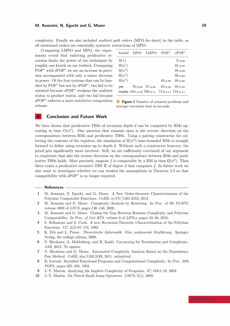
bound MPO LMPO POP∗ sPOP∗
O(1) 9\0.06
O(n1) 32\0.07
O(n2) 38\0.09
O(n3) 39\0.20
O(nk) 43\0.05 39\0.20
yes 76\0.09 57\0.05 43\0.05 39\0.07
maybe 681\0.16 700\0.11 714\0.11 718\0.11
Figure 1 Number of oriented problems and
average execution time in seconds.
Comparing LMPO and MPO, the exper-
iments reveal that enforcing predicative re-
cursion limits the power of our techniques by
roughly one fourth on our testbed. Comparing
POP∗ with sPOP∗ we see an increase in preci-
sion accompanied with only a minor decrease
in power. Of the four systems that can be han-
dled by POP∗ but not by sPOP∗, two fail to be
oriented because sPOP∗ weakens the multiset
status to product status, and two fail because
sPOP∗ enforces a more restrictive composition
scheme.
4 Conclusion and Future Work
We have shown that predicative TRSs of recursion depth d can be computed by RMs op-
erating in time O(nd). One question that remains open is the reverse direction on the
correspondence between RMs and predicative TRSs. Using a pairing constructor for col-
lecting the contents of the registers, the simulation of O(nd) time-bounded RMs is straight
forward to define using recursion up to depth d. Without such a constructor however, the
proof gets significantly more involved. Still, we are sufficiently convinced of our argument
to conjecture that also the reverse direction on the correspondence between RMs and pred-
icative TRSs holds. More precisely, suppose f is computable by a RM in time O(nd). Then
there exists a predicative recursive TRS R of degree d that computes f . In future work we
also want to investigate whether we can weaken the assumptions in Theorem 2.2 so that
compatibility with sPOP∗ is no longer required.
References
1 M. Avanzini, N. Eguchi, and G. Moser. A New Order-theoretic Characterisation of the
Polytime Computable Functions. CoRR, cs/CC/1201.2553, 2012.
2 M. Avanzini and G. Moser. Complexity Analysis by Rewriting. In Proc. of 9th FLOPS,
volume 4989 of LNCS, pages 130–146, 2008.
3 M. Avanzini and G. Moser. Closing the Gap Between Runtime Complexity and Polytime
Computability. In Proc. of 21st RTA, volume 6 of LIPIcs, pages 33–48, 2010.
4 S. Bellantoni and S. Cook. A new Recursion-Theoretic Characterization of the Polytime
Functions. CC, 2(2):97–110, 1992.
5 K. Erk and L. Priese. Theoretische Informatik: Eine umfassende Einführung. Springer
Verlag, 3te auflage edition, 2008.
6 N. Hirokawa, A. Middeldorp, and H. Zankl. Uncurrying for Termination and Complexity.
JAR, 2012. To appear.
7 N. Hirokawa and G. Moser. Automated Complexity Analysis Based on the Dependency
Pair Method. CoRR, abs/1102.3129, 2011. submitted.
8 D. Leivant. Stratified Functional Programs and Computational Complexity. In Proc. 20th
POPL, pages 325–333, 1993.
9 J.-Y. Marion. Analysing the Implicit Complexity of Programs. IC, 183:2–18, 2003.
10 J.-Y. Marion. On Tiered Small Jump Operators. LMCS, 5(1), 2009.
WST 2012
Higher-Order Interpretations and Program
Complexity∗
Patrick Baillot1 and Ugo Dal Lago2
1 LIP (UMR 5668 CNRS-ENS Lyon-INRIA-UCBL)
2 Università di Bologna & INRIA
Abstract
Polynomial interpretations and their generalizations like quasi-interpretations have been used in
the setting of first-order functional languages to design criteria ensuring statically some com-
plexity bounds on programs [3]. This fits in the area of implicit computational complexity,
which aims at giving machine-free characterizations of complexity classes. Here we extend this
approach to the higher-order setting. For that we consider the notion of simply typed term
rewriting systems [8], we define higher-order polynomial interpretations (HOPI) for them and
give a criterion based on HOPIs to ensure that a program can be executed in polynomial time.
In order to obtain a criterion which is flexible enough to validate some interesting programs using
higher-order primitives, we introduce a notion of polynomial quasi-interpretations, coupled with
a simple termination criterion based on linear types and path-like orders.
1998 ACM Subject Classification F.4.1 - Mathematical Logic, F.4.2 - Grammars and Other
Rewriting Systems
Keywords and phrases Simply-Typed Term Rewriting, Interpretations, Quasi-Interpretations,
Implicit Computational Complexity
1 Introduction
The problem of statically analyzing the performance of programs can be attacked in many
different ways. One of them consists in inferring complexity properties of programs early in
development cycle, when the latter are still expressed in high-level programming languages,
like functional or object oriented idioms. And in this scenario, results from an area known
as implicit computational complexity (ICC in the following) can be useful: they consist
in characterizations of complexity classes in terms of paradigmatic programming languages
(λ-calculus, term rewriting systems, etc.) or logical systems (proof-nets, natural deduction,
etc.), from which static analysis methodologies can be distilled. Examples are type systems,
path-orderings and variations on the interpretation method. The challenge here is defining
ICC systems which are not only simple, but also intensionally powerful: many natural
programs among those with bounded complexity, should be recognized as such by the ICC
system, i.e., are actually programs of the system.
One of the most fertile direction in ICC is indeed the one in which programs are term
rewriting systems (TRS in the following) [3, 4], whose complexity can be kept under control
by way of variations of the powerful techniques developed to check termination of TRS,
namely path orderings [7, 5], dependency pairs and the interpretation method [6]. Many
∗ This work was partially supported by the projects INRIA ARC ETERNAL and COMPLICE (ANR-08-BLANC-0211-01).
© P. Baillot and U. Dal Lago;licensed under Creative Commons License NC-ND
WST 2012: 12th International Workshop on Termination.Editor: G. Moser; pp. 20–24
P. Baillot and U. Dal Lago 21
different complexity classes have been characterized this way, from polynomial time to poly-
nomial space, to exponential time to logarithmic space. And remarkably, many of the intro-
duced characterizations are intensionally very powerful, in particular when the interpretation
method is relaxed and coupled with recursive path orderings, like in quasi-interpretations
[4].
Here, we consider one of the simplest higher-order generalizations of TRSs, namely Ya-
mada’s simply-typed term rewriting systems (STTRSs in the following), we define a system
of higher-order polynomial interpretations for them and prove that, following [3], this allows
to exactly characterize, among others, the class of polynomial time computable functions.
An extended version of this paper is available [2] which includes all proofs, together with a
description of how the proposed approach can be adapted to quasi-interpretations, in the
style of [4].
2 Simply-Typed Term Rewriting Systems
We recall here the definition of a STTRS, following [8, 1]. We will actually consider as
programs a subclass of STTRSs, basically those where rules only deal with the particular
case of a function symbol applied to a sequence of patterns. For first-order rewrite systems
this corresponds to the notion of constructor rewrite system.
We consider a denumerable set of base types, which we call data-types and we shall
denote as D or E. Types are defined by the following grammar:
A,B ::= D | A1 × · · · ×An → A.
A functional type is a type which contains an occurrence of→. Some examples of base types
are the type NAT of tally integers, and the type W2 of binary words.
We denote by F the set of function symbols (or just functions), C that of constructors
and X that of variables. Constructors c ∈ C have a type of the form D1 × · · · ×Dn → D.
Functions f ∈ F , on the other hand, can have any functional type. Variables x ∈ X can
have any type. Terms are typed and defined by the following grammar:
t, ti := xA | cA | fA | (tA1×···×An→A tA1
1 . . . tAnn )A
where xA ∈ X , cA ∈ C, fA ∈ F . We denote by T the set of terms. Observe how application
is primitive and is in general treated differently from other function symbols. This is what
make STTRSs different from ordinary TRSs.
We define the size |t| of a term t as the number of symbols (elements of F ∪ C ∪ X )
it contains. To simplify the writing of terms we will often elide their type. We will also
write (t s) for (t s1 . . . sn). Therefore any term t is of the form (. . . ((α s1) s2) . . . sk) where
k ≥ 0, α ∈ X ∪ C ∪ F . Moreover, we will use the following convention: any term t is of
the form (. . . ((s s1) s2) . . . sk) will be written ((s s1 . . . sk)). A crucial class of terms are
patterns, which in particular are used in defining rewriting rules. Formally, a pattern is a
term generated by the following grammar:
p, pi := xA | (cD1×...×Dn→D pD1
1 . . . pDnn ).
P is the set of all patterns. Observe that if a pattern has a functional type then it must
be a variable. We consider rewriting rules in the form t → s satisfying the following two
constraints:
1. t and s are terms of the same type A, FV (s) ⊆ FV (t), and any variable appears at most
once in t.
WST 2012
22 Higher-Order Interpretations and Program Complexity
2. t must have the form ((f p1 . . . pk)) where each pi for i ∈ 1, . . . , k consists of patterns only.
The rule is said to be a rule defining f, while the total number of patterns in p1, . . . , pkis the arity of the rule.
Now, a simply-typed term rewriting system is a set R of orthogonal rewriting rules such that
for every function symbol f, every rule defining f has the same arity, which is said to be the
arity of f.
We consider call-by-value reduction of STTRSs, i.e, only values will be passed as argu-
ments to functions. Formally, we say that a term is a value if either:
1. it has type D and is in the form (c v1 . . . vn), where v1, . . . , vn are themselves values.
2. it has functional type and is of the form ((f, v1 . . . vn)), where the terms in v1, . . . vn are
themselves values and the total number of terms in v1, . . . , vn is strictly smaller than the
arity of f.
We denote values as v, u and their set by V.
3 Higher-Order Polynomial Interpretations
We want to demonstrate how first-order rewriting-based techniques for ICC can be adapted
to the higher-order setting. Our goal is to devise criteria ensuring a complexity bound
on programs of first-order types but using subprograms of higher-order types. A typical
application will be to find out under which conditions a higher-order functional program
such as e.g. map, iteration or foldl, fed with a (first-order) polynomial time program
produces a polynomial time program.
As a first illustrative step we consider the approach based on polynomial interpretations
from [3], which offers the advantage of simplicity. We thus build a theory of higher-order
polynomial interpretations for STTRSs. It can be seen as a particular concrete instantiation
of the methodology proposed in [8] for proving termination by interpretation.
Higher-order polynomials (HOPs) take the form of terms in a typed λ-calculus whose
only base type is that of natural numbers. To each of those terms can be assigned a strictly
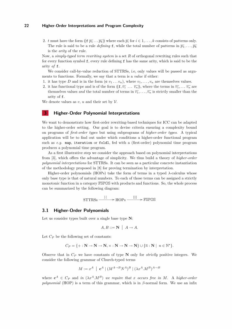
monotonic function in a category FSPOS with products and functions. So, the whole process
can be summarized by the following diagram:
STTRSs[·]
// HOPsJ·K
// FSPOS
3.1 Higher-Order Polynomials
Let us consider types built over a single base type N:
A,B ::= N | A→ A.
Let CP be the following set of constants:
CP = + : N→ N→ N,× : N→ N→ N ∪ n : N | n ∈ N⋆.
Observe that in CP we have constants of type N only for strictly positive integers. We
consider the following grammar of Church-typed terms
M := xA | cA | (MA→BNA)B | (λxA.MB)A→B
where cA ∈ CP and in (λxA.MB) we require that x occurs free in M . A higher-order
polynomial (HOP) is a term of this grammar, which is in β-normal form. We use an infix
P. Baillot and U. Dal Lago 23
notation for + and ×. We assume given the usual set-theoretic interpretation of types and
terms, denoted as JAK and JMK: if M has type A and FV (M) = xA1
1 , . . . , xAnn , then JMK
is a map from JA1K × . . . × JAnK to JAK. We denote by ≡ the equivalence relation which
identifies terms which denote the same function, e.g. we have: λx.(2 × ((3 + x) + y)) ≡
λx.(6 + (2× x+ 2× y)).
Noticeably, even if HOPs can be built using higher-order functions, the first order frag-
ment only contains polynomials:
Lemma 1. If M is a HOP of type N and such that FV (M) = y1 : N, . . . , yk : N, then
the function JMK is a polynomial function.
3.2 Semantic Interpretation.
Now, we consider a subcategory FSPOS of the category SPOS of strict partial orders as
objects and strictly monotonic total functions as morphisms. Objects of FSPOS are the
following:
N is the domain of strictly positive integers, equipped with the natural strict order ≺N ,
1 is the trivial order with one point;
if σ, τ are objects, then σ × τ is obtained by the product ordering,
σ → τ is the set of strictly monotonic total functions from σ to τ , equipped with the
following strict order: f ≺σ→τ g if for any a of σ we have f(a) ≺τ g(a).
We denote by τ the reflexive closure of ≺τ . FSPOS is a subcategory of SET with all the
necessary structure to interpret types. JAK≺ denotes the semantics of A as an object of
FSPOS. We choose to set JNK≺ = N . Notice that any element of e ∈ JAK≺ can be easily
mapped onto an element e ↓ of JAK. What about terms? Actually, FSPOS can again be
shown to be sufficiently rich:
Proposition 2. LetM be a HOP of type A with free variables xA1
1 , . . . , xAnn . Then for every
e ∈ JA1× . . .×AnK≺, there is exactly one f ∈ JAK≺ such that f ↓= JMK(e↓). Moreover, this
correspondence is strictly monotone and thus defines an element of JA1 × . . . × An → AK≺which we denote as JMK≺.
3.3 Assignments and Polynomial Interpretations
To each variable xA we associate a variable xA where A is obtained from A by replacing
each occurrence of base type by the base type N and by curryfication. We will sometimes
write x (resp. A) instead of x (resp. A) when it is clear from the context.
An assignment [ · ] is a map from C ∪ F to HOPs such that if f ∈ C ∪ F , [f ] is a closed
HOP, of type A1, . . . , An → A. Now, for t ∈ T we define [t] by induction on t:
if t ∈ X , then [t] is f ;
if t ∈ C ∪ F , [t] is already defined;
otherwise, if t = (t0 t1 . . . tn) then [t] ≡ (. . . ([t0][t1]) . . . [tn]).
Observe that in practice, computing [t] will in general require to do some β-reduction steps.
Lemma 3. If s→ t, then JtK≺ ≺ JsK≺.
As a consequence, the interpretation of terms (of base type) is itself a bound on the length
of reduction sequences:
Proposition 4. Let t be a closed term of base type D. Then [t] has type N and any
reduction sequence of t has length bounded by JtK≺.
WST 2012
24 Higher-Order Interpretations and Program Complexity
3.4 A Complexity Criterion
Proving a STTRS to have an interpretation is not enough to guarantee its time complexity to
be polynomial. To ensure that, we need to impose some constraints on the way constructors
are interpreted.
We say that the assignment [ · ] is additive if any constructor c of type D1 × · · · ×Dn →
E, where n ≥ 0, is interpreted by a HOP Mc whose semantic interpretation JMcK≺ is a
polynomial function of the form:
P (y1, . . . , yn) =
n∑
i=1
yi + γc, with γc ≥ 1.
Additivity ensures that the interpretation of first-order values is proportional to their size:
Lemma 5. Let [ · ] be an additive assignment. Then there exists γ ≥ 1 such that for any
value v of type D, where D is a data type, we have JvK≺ ≤ γ · |v|.
The base type Wn denotes the data-type of n-ary words, whose constructors are empty
and c1, . . . , cn. A function f : (0, 1∗)m → 0, 1∗ is said to be representable by a STTRS
R if there is a function symbol f of type Wm2 →W2 in R which computes f in the obvious
way. Noticeably:
Theorem 6. The functions on binary words representable by STTRSs admitting an addi-
tive polynomial interpretation are exactly the polytime functions.
Not many programs can be proved to be polytime by way of the criterion we have just
introduced. This, however, can be partially solved by switching to quasi-interpretations, as
described in [2].
References
1 Takahito Aoto and Toshiyuki Yamada. Termination of simply typed term rewriting by
translation and labelling. In Proceedings of RTA 2003, volume 2706 of LNCS. Springer,
2003.
2 Patrick Baillot and Ugo Dal Lago. Higher-order interpretations and program complexity
(long version). Available at http://hal.archives-ouvertes.fr/hal-00667816, 2012.
3 Guillaume Bonfante, Adam Cichon, Jean-Yves Marion, and Hélène Touzet. Algorithms
with polynomial interpretation termination proof. Journal of Functional Programming,
11(1):33–53, 2001.
4 Guillaume Bonfante, J.-Y. Marion, and Jean-Yves Moyen. Quasi-interpretations a way to
control resources. Theoretical Computer Science, 412(25):2776–2796, 2011.
5 Nachum Dershowitz. Orderings for term-rewriting systems. Theoretical Computer Science,
17(3):279–301, 1982.
6 D. Lankford. On proving term rewriting systems are noetherian. Technical Report MTP-3,
Louisiana Tech. University, 1979.
7 D. A. Plaisted. A recursively defined ordering for proving termination of term rewriting
systems. Technical Report R-78-943, University of Illinois, Urbana, Illinois, September
1978.
8 Toshiyuki Yamada. Confluence and termination of simply typed term rewriting systems.
In Proceedings of RTA 2001, volume 2051 of LNCS, pages 338–352. Springer, 2001.
Recent Developments in the Matchbox
Termination Prover
Alexander Bau∗, Tobias Kalbitz, Maria Voigtländer, and Johannes
Waldmann
Fakultät IMN, HTWK Leipzig, Germany
Abstract
We report on recent and ongoing work on the Matchbox termination prover:
a constraint compiler that transforms a Boolean-valued Haskell function into a Boolean sat-
isfiability problem (SAT),
a constraint solver for real and arctic matrix constraints that is using evolutionary optimiza-
tion, and is running on massively parallel (graphics) hardware.
1998 ACM Subject Classification F.1.1 - Models of Computation
Keywords and phrases Rewriting, Termination, Constraint Programming
1 Introduction
The program Matchbox [11] originally proved termination of string rewriting, using the
method of match bounds [6]. The domain was extended to term rewriting, by adding proof
methods of dependency pairs [1], matrix interpretations over the integers [4] and over arctic
numbers [9].
These methods are typical instances of the following scheme: to automatically find a
proof of termination, one solves constraint satisfaction problems. E.g., the precedence of
function symbols, or the coefficients of polynomials and matrices, are constrained by the
condition that the resulting path order, polynomial order, or matrix order, respectively, is
compatible with a given rewriting system.
The constraint system could be solved by
by domain-specific methods (e.g., Matchbox computes a certificate for match-boundedness
by completion of automata),
by generic search (exhaustively, randomly, or directed by some fitness function),
by transformation to another constraint domain (e. g., Matchbox transforms integer
and arctic polynomial inequalities to a Boolean satisfiability problem, and solves it with
Minisat [3]).
In the present paper, we report on recent and ongoing work to
extract a general framework for constraint programming by automatic transformation to
SAT,
and (independently) add a domain-specific solver for real and arctic matrix constraints
that is using evolutionary optimization, and is running on massively parallel (graphics)
hardware.
∗ Alexander Bau is supported by an ESF grant
© A. Bau, T. Kalbitz, M. Voigtländer, and J. Waldmann;licensed under Creative Commons License NC-ND
WST 2012: 12th International Workshop on Termination.Editor: G. Moser; pp. 25–28
26 Recent Developments in the Matchbox Termination Prover
2 A Constraint Compiler
The idea behind constraint programming is to separate specification (encoded as constraint
system) from implementation (the constraint solver). The obvious choice for the specifica-
tion language is mathematical logic, equivalently, a pure (i.e. side-effect free) functional
programming language like Haskell. A constraint system c can be seen as a function with
type c : U → Bool, where the solution is an object s ∈ U such that c(s) is True.
There are clever solvers for the case that U ′ = Bool∗, and c′ is given by a formula in
propositional logic. But typically, the application domain U is different. The translation
from U to U ′ can be done manually by the programmer, or automatically, by some tool.
The satchmo library (http://hackage.haskell.org/package/satchmo) used in Matchbox
is an example for the “manual” approach. It is an embedded (in Haskell) domain specific
language for the generation of SAT constraints. Several termination researchers built and
published similar libraries for other host languages (Ocaml, Java). These interweave the
generation of the boolean formula with the declaration of the constraint system in the host
language. E.g., satchmo generates the formula as a side effect represented by a suitable State
monad. Actually these are different processes and should be separated from each other.
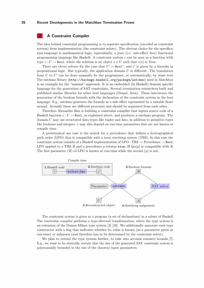
Therefore Alexander Bau is building a constraint compiler that inputs source code of a
Haskell function c : U → Bool, as explained above, and produces a satchmo program. The
domain U may use structured data types like tuples and lists, in addition to primitive types
like booleans and integers. c may also depend on run-time parameters that are not known at
compile time.
A prototypical use case is the search for a precedence that defines a lexicographical
path order (LPO) that is compatible with a term rewriting system (TRS). In this case the
constraint system consists of a Haskell implementation of LPO : TRS→ Precedence→ Bool.
LPO applied to a TRS R and a precedence p returns true, iff lpo(p) is compatible with R.
The first parameter (R) of LPO is known at run-time while the second (p) is not.
c hs2satchmo c′
Parameter satchmo
U
B
SAT solver
A
1.Haskell code 2.Satchmo code 3.Boolean formula
4.Satisfying assignment5.Reconstructed object
Compile time
The constraint system is given as a program (a set of declarations) in a subset of Haskell.
The constraint compiler performs a type-directed transformation, where the type system is
an extension of the Damas-Milner type system [2] [10]. We additionally annotate each type
constructor with a flag that indicates whether its value is known (as a parameter given at
run-time) or unknown (and therefore has to be determined by the constraint solver).
We plan to extend the type system further, to take into account resource bounds [7].
E.g., we want to be statically certain that the size of the generated SAT constraint system is
polynomially bounded in the size of the (known) input parameters.
A. Bau, T. Kalbitz, M. Voigtländer, and J. Waldmann 27
3 Massively Parallel Constraint Solving
A constraint satisfaction problem can be converted into an optimization problem that is
solved by evolutionary algorithms. For the domain of matrix interpretations, this approach
was used by Dieter Hofbauer’s termination prover MultumNonMulta (2006, 2007), see also
[5]. We return to it now, since it allows for massive parallelisation.
In the context of numerical constraint solving by randomized, directed search, parallel
processing is applicable because
basic operations (on numbers) can be executed fast
domain specific operations (matrix multiplications) can be sped up by parallelism (multi-
plication of n dimensional square matrices, using n2 cores and n time)
evolutionary search strategies can be sped up again, by treating several individuals in
parallel (e.g., computing their fitness values)
General Purpose Graphical Processing Units (GPGPUs) provide massively parallel
processing at affordable prices. Tobias Kalbitz and Maria Voigtländer are implementing
matrix constraint solvers for CUDA capable graphics cards. CUDA (Compute Unified Device
Architecture) [8] is a parallel programming model for NVIDIA’s GPGPUs.
The following approach is used to find a strictly monotone matrix interpretation of
dimension d that is compatible with a string rewriting system R over alphabet Σ (weakly
compatible with each rule, and strictly compatible with at least one rule):
A population consists of several individuals, each individual is a matrix interpretation,
that is, a mapping [·] : Σ → Nd×d, where for each a ∈ Σ, the first column of [a] is
(1, 0, . . . , 0)T , and the last row of [a] is (0, . . . , 0, 1). This condition ensures monotonicity.
The fitness of an interpretation [·] is∑max(0, [r]p,q− [l]p,q)
2 | (l, r) ∈ R, 1 ≤ p, q ≤ d,
plus some very large penalty in case that ¬∃(l, r) ∈ R : [l]1,d > [r]1,d. Lower fitness values
are better, and value zero indicates that compatibility holds.
An individual with fitness > 0 is changed by a large mutation: we randomly pick some
(l, r) ∈ R, 1 ≤ p, q ≤ d such that [l]p,q < [r]p,q, and we choose randomly a sequence
of indices p = p0, p1, . . . , pn = q with n = |l|, and then increase each [ai]pi−1,pi by one,
where l = a1 . . . an. This ensures that [l]p,q increases.
Next, this individual undergoes a series of small mutations where for any a ∈ Σ, 1 ≤
i, j ≤ d, the entry at [a]i,j is modified. We try sereval small mutations, until we find one
that decreases fitness, and then repeat. The total number of small mutations is bounded.
The resulting individual is placed back into the population, removing another individual
of larger fitness.
Example 1. With 1000 individuals, and 100 small steps after each large step, we find a
compatible 5-dimensional interpretation for a2b2 → b3a3 (Problem z001) with < 30.000 large
steps with probability > 50%. Of course, the total runtime is not bounded, as the evolution
may go into a dead-end. So it is better to re-start than to wait.
Applying this idea to rational, and arctic, numbers, we meet the following challenges:
Real numbers are approximated by rational (“floating point” values), thus results of
comparisons may be wrong. The solution is to introduce a “grid” for rounding input values,
e.g. use only integer multiples of 1/2, or 1/10, say.
A fine grid implies a smooth objective function, and this may help evolutionary algorithms.
On the other hand, a coarse grid reduces the search space, and may increase the chance that
we find a solution by luck.
Note that we do not need a grid for arctic numbers, since we can use arctic integers.
WST 2012
28 Recent Developments in the Matchbox Termination Prover
On typical CUDA cards, a large number of compute cores is available (e.g., 512). They
can only be used efficiently if the data that they process is stored in fast (thread-(block-)local)
memory. The amount of such memory is severely limited (e.g., 16 kByte total, resulting in
300 byte per core)
CUDA cards are programmed in (a dialect of) C. This allows fine-grained control, but
is highly impractical for large-scale programming. Therefore, we are isolating the low-level
details in a C library, and provide it with an interface to Haskell, where we implement global
flow of control. Still it is important that data stays on the card’s memory, since transport to
and from the host computer’s memory is slow.
4 Future plans
We stress that the above is a report on ongoing work.
We plan to have an implementation ready for the termination competition in 2012. The
code will be open-sourced.
Since the hardware of the competition platform does not include a GPGPU, we will run
Matchbox/CUDA remotely.
References
1 Thomas Arts and Jürgen Giesl. Termination of term rewriting using dependency pairs.
Theoretical Computer Science, 236(1-2):133–178, 2000.
2 Luís Damas and Robin Milner. Principal type-schemes for functional programs. In POPL,
pages 207–212, 1982.
3 Niklas Eén and Armin Biere. Effective preprocessing in sat through variable and clause
elimination. In Fahiem Bacchus and Toby Walsh, editors, SAT, volume 3569 of Lecture
Notes in Computer Science, pages 61–75. Springer, 2005.
4 Jörg Endrullis, Johannes Waldmann, and Hans Zantema. Matrix interpretations for proving
termination of term rewriting. J. Autom. Reasoning, 40(2-3):195–220, 2008.
5 Andreas Gebhardt, Dieter Hofbauer, and Johannes Waldmann. Matrix evolutions. In Dieter
Hofbauer and Alexander Serebrenik, editors, Proc. Workshop on Termination, Paris, 2007.
6 Alfons Geser, Dieter Hofbauer, and Johannes Waldmann. Match-bounded string rewriting
systems. Appl. Algebra Eng. Commun. Comput., 15(3-4):149–171, 2004.
7 Jan Hoffmann. Types with Potential: Polynomial Resource Bounds via Automatic Amor-
tized Analysis. PhD thesis, Ludwig-Maximilians-Universiät München, 2011.
8 David B. Kirk and Wne mei W. Hwu. Programming Massively Parallel Processors. Morgan
Kaufmann Publishers, 2010.
9 Adam Koprowski and Johannes Waldmann. Max/plus tree automata for termination of
term rewriting. Acta Cybern., 19(2):357–392, 2009.
10 Alan Mycroft. Incremental polymorphic type checking with update. In LFCS, pages 347–
357, 1992.
11 Johannes Waldmann. Matchbox: A tool for match-bounded string rewriting. In Vincent
van Oostrom, editor, RTA, volume 3091 of Lecture Notes in Computer Science, pages 85–94.
Springer, 2004.
The recursive path and polynomial ordering∗
Miquel Bofill1, Cristina Borralleras2, Enric Rodríguez-Carbonell3,
and Albert Rubio3
1 Universitat de Girona, Spain
2 Universitat de Vic, Spain
3 Universitat Politècnica de Catalunya, Barcelona, Spain
Abstract
In most termination tools two ingredients, namely recursive path orderings (RPO) and polyno-
mial interpretation orderings (POLO), are used in a consecutive disjoint way to solve the final
constraints generated from the termination problem.
We present a simple ordering that combines both RPO and POLO and defines a family of
orderings that includes both, and extends them with the possibility of having, at the same time,
an RPO-like treatment for some symbols and a POLO-like treatment for the others.
The ordering is extended to higher-order terms, providing an automatable use of polynomial
interpretations in combination with beta-reduction.
1 Introduction
Term orderings have been extensively used in termination proofs of rewriting. They are used
both in direct proofs of termination showing decreasingness of every rule or as ingredients for
solving the constraints generated by other methods like the Dependency Pair approach [1]
or the Monotonic Semantic Path Ordering [4].
The most widely used term orderings in automatic termination tools are the recursive
path ordering (RPO) and the polynomial ordering (POLO). Almost all known tools im-
plement these orderings. RPO and POLO are incomparable, so that they are used in a
sequential way, first trying one method (maybe under some time limit) and, in case of
failure, trying the other one afterwards.
As an alternative to this sequential application we propose a new ordering that combines
both RPO and POLO. The new family of orderings, called RPOLO, includes strictly both
RPO and POLO as well as the sequential combination of both. Our approach is based on
splitting the set of symbols into those handled in an RPO-like way (called RPO-symbols)
and those that are interpreted using a polynomial interpretation (called POLO-symbols).
In this paper, only linear polynomial interpretations are considered. These interpretations
are never applied to terms headed by an RPO-symbol. Instead, the term is interpreted
as a new variable (labeled by the term). This is crucial to be able to extend the ordering
to the higher-order case, since applying polynomial interpretations to beta-reduction is not
easy. However, the introduction of different unrelated variables for every term makes us lose
stability under substitutions and (weak) monotonicity. To avoid that, a context relating the
variables is introduced, but then a new original proof of well-foundedness is needed.
Matrix interpretations [8, 7], have recently been adopted as the third alternative to
define term orderings. As future work, it would be interesting to study if our results can
be generalized to matrix interpretations and to more general interpretations fulfilling some
required properties1.
∗ This work has been partially supported by the Spanish MEC/MICINN under grants TIN2008-04547and TIN 2010-68093-C02-01
1 We would like to thank the anonymous referee that pointed us this possible extension
© M. Bofill, C. Borralleras, E. Rodríguez-Carbonell, and A. Rubio;licensed under Creative Commons License NC-ND
WST 2012: 12th International Workshop on Termination.Editor: G. Moser; pp. 29–33
30 The recursive path and polynomial ordering
Although the new ordering is strictly more powerful than its predecessors and thus
examples that can be handled by RPOLO and neither by RPO nor by POLO can be cooked,
in practice, there is no real gain when using RPOLO on the first-order examples coming
from the Termination Problem Data Base.
Due to this, we show its practical usefulness by extending it, using the same techniques
as for the higher-order recursive path ordering [10] (HORPO), to rewriting on simply typed
higher-order terms union beta-reduction. The resulting ordering, called HORPOLO, can
hence be used to prove termination of the so called Algebraic Functional Systems [9] (AFS),
and provides an automatable termination method that allows the user to have polynomial
interpretations on some symbols in a higher-order setting. Note that, although some polyno-
mial interpretations for higher-order rewrite systems à la Nipkow where extensively studied
in [11], it is unclear how to implement those techniques in an automatic tool.
Due to the space limitations we have not included here the definitions of the higher-order
version of the ordering, but it is the natural extension following the same ideas applied to
extend RPO to HORPO (for a full version of this work see [3]).
2 The recursive path and polynomial ordering (RPOLO)
Here we present the ordering for first-order terms. Let F be a signature split into two sets
FPOLO and FRPO. We have a precedence F on FRPO and a polynomial interpretation I
over the non-negative integers Z+ for the terms in T (F ,X ). Moreover, the interpretation I
is defined by a linear interpretation fI with coefficients in Z+ for every symbol f in FPOLO
and a variable xs for every term s with top symbol in FRPO:
I(s) =
fI(I(s1), . . . , I(sn)) if s = f(s1, . . . , sn) and f ∈ FPOLOxs otherwise
In order to handle these introduced variables xs, we define a context information to be
used when comparing the interpretations. In what follows a (polynomial) context is a set of
constraints of the form x ≥ E where x is a variable and E is a linear polynomial expression
over Z+. Let us now show the way contexts are used when comparing polynomials.
Definition 1. Let C be a context. The relation→C on linear polynomial expressions over
Z+ is defined by the rules P + x→C P + E for every x ≥ E ∈ C.
Let p and q be linear polynomial expressions over Z+. Then p >C q (resp. p ≥C q) if
there is some u such that p −→q =C u > q (resp. p −→q =
C u ≥ q).
We use here (the reflexive closure of) a parallel rewriting step −→q =C instead of the tran-
sitive closure of →C because it simplifies the proofs without losing any power.
The following three mutually recursive definitions introduce respectively the context
C(S) of a set of terms S, the ordering ≻RPOLO and the compatible quasi-ordering ⊒RPOLO.
Definition 2. Let S be a set of terms u such that top(u) 6∈ FPOLO. The context C(S) is
defined as the union of
1. xu ≥ E+1 for all u ∈ S and for all linear polynomial expressions E over Z+ and variables
xv1 , . . . , xvn such that u ≻RPOLO vi for all i ∈ 1, . . . , n.
2. xu ≥ xv for all u ∈ S and all v such that u ⊒RPOLO v and top(v) ∈ FRPO.
Note that C(s) can be infinite. For this reason, in practice, when comparing a pair of
terms s and t we only generate the part of C(s) that is needed. This part is chosen by
inspecting t.
M. Bofill, C. Borralleras, E. Rodríguez-Carbonell, and A. Rubio 31
Definition 3. s ⊒RPOLO t iff
1. s = t ∈ X , or
2. s = f(s1, . . . , sn) and
a. f ∈ FPOLO, I(s) ≥C(s) I(t) or
b. t = g(t1, . . . , tn), f, g ∈ FRPO, f =F g and
i. stat(f) = mul and s1, . . . , sn(⊒RPOLO)mont1, . . . , tn, or
ii. stat(f) = lex and 〈s1, . . . , sn〉(⊒RPOLO)mon〈t1, . . . , tn〉.
Definition 4. s = f(s1, . . . , sn) ≻RPOLO t iff
1. f ∈ FPOLO and I(s) >C(s) I(t), or
2. f ∈ FRPO, and
a. si RPOLO t for some i ∈ 1, . . . , n, or
b. t = g(t1, . . . , tm), g ∈ FPOLO and s ≻RPOLO u for all u ∈ Acc(t), or
c. t = g(t1, . . . , tm), g ∈ FRPO and
i. f ≻F g and s ≻RPOLO ti for all i ∈ 1, . . . ,m, or
ii. f =F g, stat(f) = mul and s1, . . . , sn(≻RPOLO)mult1, . . . , tm, or
iii. f =F g, stat(f) = lex, 〈s1, . . . , sn〉(≻RPOLO)lex〈t1, . . . , tm〉 and s ≻RPOLO ti for all
i ∈ 1, . . . ,m,
where s RPOLO t iff s ≻RPOLO t or s ⊒RPOLO t and Acc(s) is defined as u | xu ∈ Var(I(s))
and, to ease the reading, C(s) denotes C(Acc(s)).
Note that ordering keeps the flavor of the RPO definition, but adding some cases to
handle the terms headed by polynomially interpreted symbols.
Now, we provide some examples of comparisons between terms that are included in our
ordering and are neither included in RPO nor in POLO, i.e., using (linear) integer polynomial
interpretations. In fact, since we consider constraints including both strict and non-strict
literals, what we show is that they are included in the pair (≻RPOLO,RPOLO).
Example 5. Consider the following constraint consisting of three literals:
H(f(g(g(x)), y), x) > H(f(g(y), x), f(g(y), x))
H(x, g(y)) ≥ H(y, x)
f(g(x), y) ≥ f(y, x)
The first literal cannot be proved by RPO since f(g(g(x)), y) cannot be proved larger than
f(g(y), x) as no argument of the former is greater than g(y). The constraints cannot be
proved terminating by an integer polynomial interpretation either.
Let us prove it using RPOLO. We takeH ∈ FRPO with stat(H) = mul and f, g ∈ FPOLOwith fI(x, y) = x+ y and gI(x) = x+ 1.
For the first literal, applying case 4.2(c)ii, we need to prove f(g(g(x)), y), x(≻RPOLO
)mulf(g(y), x), f(g(y), x), which holds since f(g(g(x)), y) ≻RPOLO f(g(y), x) by case 4.1 as
I(f(g(g(x)), y)) = xx + xy + 2 > xx + xy + 1 = I(f(g(y), x)). The proof of the other two
literals reuses part of the previous argument.
Let us now show an example where we need symbols in FRPO occurring below symbols
that need to be in FPOLO. Moreover, in this example a non-trivial use of the context is also
necessary.
Example 6. Consider the following constraint coming from a termination proof:
f(0, x) ≥ x
f(s(x), y) ≥ s(f(x, f(x, y)))
H(s(f(s(x), y)), z) > H(s(z), s(f(x, y)))
WST 2012
32 The recursive path and polynomial ordering
The third literal needs H and s to be in FPOLO. To hint this fact, note that we cannot
remove s and, in that case, no argument in H(s(f(s(x), y)), z) can be greater than or equal
to s(z). On the other hand, since due to the third literal, s cannot be removed and needs
a non-zero coefficient for its argument, there is no polynomial interpretation for f fulfilling
the first two literals, i.e., f must be in FRPO.
Therefore, we take H, s ∈ FPOLO with HI(x, y) = x+y and sI(x) = x+1, and f ∈ FRPOwith stat(f) = lex.
The first literal holds by case 4.2a. For the second one, f(s(x), y) ≻RPOLO s(f(x, f(x, y)))
is proved by applying case 4.2b which requires f(s(x), y) ≻RPOLO f(x, f(x, y)). We apply
then case 4.2(c)iii, showing s(x) ≻RPOLO x, by case 4.1, since I(s(x)) = xx + 1 > xx = I(x),
and f(s(x), y) ≻RPOLO x and f(s(x), y) ≻RPOLO f(x, y) for the arguments. The first one holds
by applying cases 4.2a and 4.1 consecutively, and the second one by case 4.2(c)iii as before.
Finally, for the third literal we apply case 4.1, since
xf(s(x),y) + xz + 1→xf(s(x),y)≥xf(x,y)+2 xf(x,y) + 2 + xz + 1 > xz + xf(x,y) + 2
Note that xf(s(x),y) ≥ xf(x,y) + 2 belongs to the context of H(s(f(s(x), y)), z) since we have
f(s(x), y) ≻RPOLO s(f(x, y)) and I(s(f(x, y))) = xf(x,y) + 1.
Let us mention that, although in the previous example we have used the context, in all
non cooked examples we have tried the context is not used. However, the context is still
necessary, since otherwise we can not prove neither stability under substitutions nor (weak)
monotonicity.
HORPOLO has been implemented as base ordering in THOR-1.0 2, a higher-order ter-
mination prover based on the monotonic higher-order semantic path ordering [6].
The implementation of HORPOLO is done by translating the ordering constraints s > t
and s ≥ t into problems in SAT modulo non-linear integer arithmetic (NIA) which is handled
by the Barcelogic [2, 5] SMT-solver.
Just to hint on the power of the extension of the ordering to the higher-order case we
provide an example that cannot be proved with other existing methods.
Example 7. Let nat be a data type, F = s : [nat]→ nat, 0 : []→ nat, dec : [nat×nat]→
nat, grec : [nat×nat×nat× (nat→ nat→ nat)]→ nat,+ : [nat×nat]→ nat, log2 : [nat×
nat]→ nat, sumlog : [nat]→ nat and X = x : nat, y : nat, u : nat, F : nat→ nat→ nat.
Consider the following set of rules:
dec(0, x) → 0
dec(x, 0) → x
dec(s(x), s(y)) → dec(x, y)
grec(0, d, u, F ) → u
grec(s(x), s(y), u, F ) → grec(dec(x, y), s(y),@(@(F, u), x), F )
2 See http://www.lsi.upc.edu/~albert/term.html
M. Bofill, C. Borralleras, E. Rodríguez-Carbonell, and A. Rubio 33
0 + x → x
s(x) + y → s(x+ y)
quad(0) → 0
quad(s(x)) → s(s(s(s(quad(x)))))
sqr(x) → sqrp(p(x, 0))
sqrp(p(0, 0)) → 0
sqrp(p(s(s(x)), y)) → sqrp(p(x, s(y)))
sqrp(p(0, s(y))) → quad(sqrp(p(s(y), 0)))
sqrp(p(s(0), y)) → quad(sqrp(p(y, 0))) + s(quad(y))
sumsqr(x) → grec(x, s(s(0)), 0, λz1 : nat.λz2 : nat.sqr(s(z2)) + z1)
The first rules define a tail recursive generalized form of the Gödel recursor where we can
decrease in any given fixed amount at every recursive call. Using it, the rules compute the
square root using the recurrence x2 = 4(x div 2)2 when x is even and x2 = 4(x div 2)2 +
4(x div 2) + 1 when x is odd. Note that in the square definitions the even/odd checking is
done along with the computation. To be able to handle this example we need to introduce
the symbol p, which allows us to have sqrp ∈ FRPO and p ∈ FPOLO.
Some more examples as well as all details and proofs can be found in [3].
References
1 T. Arts and J. Giesl. Termination of Term Rewriting Using Dependency Pairs. Theoretical
Computer Science, 236(1-2):133-178, 2000.
2 M. Bofill, R. Nieuwenhuis, A. Oliveras, E. Rodríguez-Carbonell and A. Rubio. The Barce-
logic SMT Solver. In Proc. 20th International Conference on Computer Aided Verification
(CAV). Springer LNCS 5123, pp. 294–298, 2008.
3 M. Bofill, C. Borralleras, E. Rodríguez-Carbonell, and A. Rubio. The recursive path and
polynomial ordering for first-order and higher-order terms. Journal submission, 2011.
4 C. Borralleras, M. Ferreira and A. Rubio. Complete monotonic semantic path orderings.
In Proc. 17th International Conference on Automated Deduction (CADE). Springer, LNAI
1831, pp. 346–364, 2000.
5 C. Borralleras, S. Lucas, E. Rodríguez-Carbonell, A. Oliveras and A. Rubio. SAT Modulo
Linear Arithmetic for Solving Polynomial Constraints. Journal of Automated Reasoning.
Springer, 2012.
6 C. Borralleras and A. Rubio. A Monotonic Higher-Order Semantic Path Ordering. In
Proceedings of the 8th International Conference on Logic for Programming, Artificial Intel-
ligence (LPAR), volume 2250 of LNAI, pages 531–547, La Havana (Cuba), December 2001.
Springer.
7 J. Endrullis, J. Waldmann and H. Zantema. Matrix interpretations for proving termination
of term rewriting. Journal of Automated Reasoning, 40(2–3):195–220, 2008.
8 D. Hofbauer and J. Waldmann. Termination of string rewriting with matrix interpretations.
In Proc. 17th International Conference on Rewriting Techniques and Applications (RTA
2006), LNCS 4098, pp. 328–342, 2006.
9 J.-P. Jouannaud and M. Okada. A computation model for executable higher-order algebraic
specification languages. In Proceedings of the 6th Annual IEEE Symposium on Logic in
Computer Science (LICS), pp. 350–361. IEEE Computer Society Press, 1991.
10 J.-P. Jouannaud and A. Rubio. Polymorphic higher-order recursive path orderings. Journal
of the ACM, 54(1):1-48, 2007.
11 J. van de Pol. Termination of Higher-order Rewrite Systems. PhD. Thesis, Utrecht Uni-
versity, 1996.
WST 2012
Proving Termination of Java Bytecode with Cyclic
Data∗
Marc Brockschmidt, Richard Musiol, Carsten Otto, and Jürgen
Giesl
LuFG Informatik 2, RWTH Aachen University, Germany
Abstract
In earlier work, we developed a technique to prove termination of Java Bytecode (JBC) automat-ically: first, JBC programs are automatically transformed to term rewrite systems (TRSs) andthen, existing methods and tools are used to prove termination of the resulting TRSs. In thispaper, we extend our technique in order to prove termination of algorithms on cyclic data suchas cyclic lists or graphs automatically. We implemented our technique in the tool AProVE andperformed extensive experiments to evaluate its practical applicability.
1998 ACM Subject Classification D.1.5 - Object-oriented Programming, D.2.4 - Software/Pro-gram Verification, D.3.3 - Language Constructs and Features, F.3.1 - Specifying and Verifying andReasoning about Programs, F.4.2 - Grammars and Other Rewriting Systems, I.2.2 - AutomaticProgramming
Keywords and phrases Termination, Java Bytecode, Cyclic Data
1 Introduction
Most techniques for proving termination of imperative languages synthesize ranking functions(e.g., [6, 13]) and localize the termination test using Ramsey’s theorem [10, 14]. For instance,such techniques are used in the tools Terminator [2, 7] and LoopFrog [9] to analyze terminationof C programs. The heap is usually abstracted to integers using separation logic, cf. e.g. [11].
On the other hand, there also exist transformational approaches which automaticallytransform imperative programs to TRSs or to (constraint) logic programs. They allow tore-use the existing techniques and tools from term rewriting or logic programming also fortermination of imperative programs. A tool to analyze C by a transformation to TRSs waspresented in [8] and the tools Julia [15] and COSTA [1] prove termination of Java Bytecode
(JBC) via a transformation to constraint logic programs. To deal with the heap, they use anabstraction to integers and represent objects by their path length (i.e., by the length of themaximal path obtained by following the fields of objects).
We presented a technique for termination of Java via a transformation to TRSs in[3, 4, 5, 12]. In contrast to other approaches for termination of imperative programs, wehandle the heap by an abstraction to terms. In this paper, we extend our technique toalso handle algorithms whose termination depends on the traversal or manipulation ofcyclic objects. Up to now, transformational approaches could not deal with such programs.Our termination technique works in two steps: first, a JBC program is transformed into atermination graph, which is a finite representation of all possible program runs. This graphtakes all sharing effects into account. In the second step, a TRS is generated from the graph.
∗ Supported by the DFG grant GI 274/5-3
© M. Brockschmidt, R. Musiol, C. Otto, and J. Giesl;licensed under Creative Commons License NC-ND
WST 2012: 12th International Workshop on Termination.Editor: G. Moser; pp. 34–38
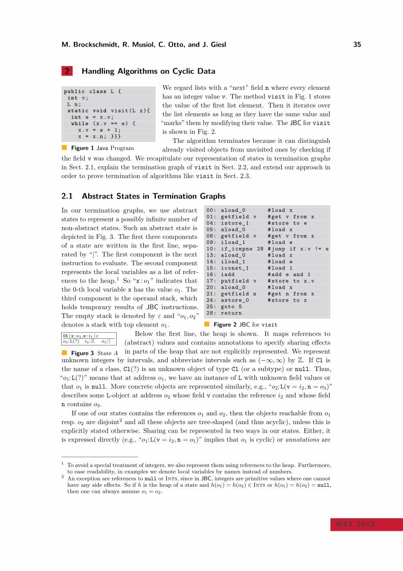
M. Brockschmidt, R. Musiol, C. Otto, and J. Giesl 35
2 Handling Algorithms on Cyclic Data
public class L int v;L n;static void visit(L x)
int e = x.v;while (x.v == e)
x.v = e + 1;x = x.n;
Figure 1 Java Program
We regard lists with a “next” field n where every elementhas an integer value v. The method visit in Fig. 1 storesthe value of the first list element. Then it iterates overthe list elements as long as they have the same value and“marks” them by modifying their value. The JBC for visit
is shown in Fig. 2.The algorithm terminates because it can distinguish
already visited objects from unvisited ones by checking ifthe field v was changed. We recapitulate our representation of states in termination graphsin Sect. 2.1, explain the termination graph of visit in Sect. 2.2, and extend our approach inorder to prove termination of algorithms like visit in Sect. 2.3.
2.1 Abstract States in Termination Graphs
00: aload_0 #load x01: getfield v #get v from x04: istore_1 #store to e05: aload_0 #load x06: getfield v #get v from x09: iload_1 #load e10: if_icmpne 28 #jump if x.v != e13: aload_0 #load x14: iload_1 #load e15: iconst_1 #load 116: iadd #add e and 117: putfield v #store to x.v20: aload_0 #load x21: getfield n #get n from x24: astore_0 #store to x25: goto 528: return
Figure 2 JBC for visit
In our termination graphs, we use abstractstates to represent a possibly infinite number ofnon-abstract states. Such an abstract state isdepicted in Fig. 3. The first three componentsof a state are written in the first line, sepa-rated by “|”. The first component is the nextinstruction to evaluate. The second componentrepresents the local variables as a list of refer-ences to the heap.1 So “x : o1” indicates thatthe 0-th local variable x has the value o1. Thethird component is the operand stack, whichholds temporary results of JBC instructions.The empty stack is denoted by ε and “o1, o2”denotes a stack with top element o1.
05 |x :o1,e : i1 |εo1:L(?) i1:Z o1
Figure 3 State A
Below the first line, the heap is shown. It maps references to(abstract) values and contains annotations to specify sharing effectsin parts of the heap that are not explicitly represented. We represent
unknown integers by intervals, and abbreviate intervals such as (−∞,∞) by Z. If Cl isthe name of a class, Cl(?) is an unknown object of type Cl (or a subtype) or null. Thus,“o1:L(?)” means that at address o1, we have an instance of L with unknown field values orthat o1 is null. More concrete objects are represented similarly, e.g., “o2:L(v = i2, n = o3)”describes some L-object at address o2 whose field v contains the reference i2 and whose fieldn contains o3.
If one of our states contains the references o1 and o2, then the objects reachable from o1resp. o2 are disjoint2 and all these objects are tree-shaped (and thus acyclic), unless this isexplicitly stated otherwise. Sharing can be represented in two ways in our states. Either, itis expressed directly (e.g., “o1:L(v = i2, n = o1)” implies that o1 is cyclic) or annotations are
1 To avoid a special treatment of integers, we also represent them using references to the heap. Furthermore,to ease readability, in examples we denote local variables by names instead of numbers.
2 An exception are references to null or Ints, since in JBC, integers are primitive values where one cannothave any side effects. So if h is the heap of a state and h(o1) = h(o2) ∈ Ints or h(o1) = h(o2) = null,then one can always assume o1 = o2.
WST 2012
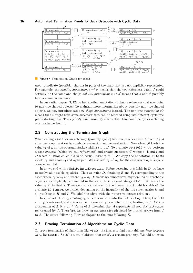
36 Automated Termination Proofs for Java Bytecode with Cyclic Data
05 |x :o1,e : i1 |εo1:L(?) i1:Z o1
A
06 |x :o1,e : i1 |o1
o1:L(?) i1:Z o1
B
06 |x :null,e : i1 |null
C
06 |x :o2,e : i1 |o2
o2:L(v= i2, n =o3)o3 : L(?) i1 : Z i2 : Z
o2,o3 o2%$o3 o2=?o3
D06 |x :o2,e : i1 |o2
o2:L(v= i2, n =o3)o3 : L(?) i1 : Z i2 : Z
o2,o3 o2%$o3
E
06 |x :o2,e : i1 |o2
o2:L(v= i2, n =o2)i1:Z i2:Z
F
10 |x :o2,e : i1 | i1, i2o2:L(v= i2, n =o3) o2%$o3
o3:L(?) i1:Z i2:Z o2,o3
G
05 |x :o2,e : i1 |εo2:L(v= i4, n =o2) i3:Z
K
10 |x :o2,e : i1 | i1, i2o2: L(v = i2, n = o3) o2%$o3
o3:L(?) i1:Z i2:Z o2,o3
H
10 |x :o2,e : i1 | i1, i1o2:L(v= i1, n =o3)o3:L(?) i1:Z
o2,o3 o2%$o3
I
10 |x :o2,e : i1 | i1, i2o2:L(v= i2, n =o2)i1:Z i2:Z
L
05 |x :o3,e : i1 |εo3:L(?) i1:Z o3
J
i1 = i2i4 = i1 +1
i1 6= i2
i1 6= i2i1
= i2
i3 = i1 +1
Figure 4 Termination Graph for visit
used to indicate (possible) sharing in parts of the heap that are not explicitly represented.For example, the equality annotation o =? o′ means that the two references o and o′ couldactually be the same and the joinability annotation o %$ o′ means that o and o′ possiblyhave a common successor.
In our earlier papers [3, 12] we had another annotation to denote references that may pointto non-tree-shaped objects. To maintain more information about possibly non-tree-shapedobjects, we now introduce two new shape annotations instead. The non-tree annotation o♦
means that o might have some successor that can be reached using two different cycle-freepaths starting in o. The cyclicity annotation o means that there could be cycles includingo or reachable from o.
2.2 Constructing the Termination Graph
When calling visit for an arbitrary (possibly cyclic) list, one reaches state A from Fig. 4after one loop iteration by symbolic evaluation and generalization. Now aload_0 loads thevalue o1 of x on the operand stack, yielding state B. To evaluate getfield v, we performa case analysis (which we call refinement) and create successors C where o1 is null andD where o1 (now called o2) is an actual instance of L. We copy the annotation to itsn-field o3 and allow o2 and o3 to join. We also add o2 =? o3, for the case where o2 is a cyclicone-element list.
In C, we end with a NullPointerException. Before accessing o2’s fields in D, we haveto resolve all possible equalities. Thus we refine D, obtaining E and F , corresponding to thecases where o2 6= o3 and where o2 = o3. F needs no annotations anymore, as all reachableobjects are completely represented in the state. In E we evaluate getfield, retrieving thevalue i2 of the field v. Then we load e’s value i1 on the operand stack, which yields G. Toevaluate if_icmpne, we branch depending on the inequality of the top stack entries i1 andi2, resulting in H and I. We label the edges with the respective integer relations.
In I, we add 1 to i1, creating i3, which is written into the field v of o2. Then, the fieldn of o2 is retrieved, and the obtained reference o3 is written into x, leading to J . As J isa renaming of A, it is an instance of A, meaning that A represents all non-abstract statesrepresented by J . Therefore, we draw an instance edge (depicted by a thick arrow) from Jto A. The states following F are analogous to the ones following E.
2.3 Proving Termination of Algorithms on Cyclic Data
To prove termination of algorithms like visit, the idea is to find a suitable marking property
M ⊆ Instances. So M is a set of objects that satisfy a certain property. We add an extra
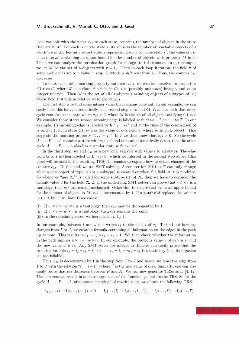
M. Brockschmidt, R. Musiol, C. Otto, and J. Giesl 37
local variable with the name cM to each state, counting the number of objects in the statethat are in M . For each concrete state s, its value is the number of reachable objects of swhich are in M . For an abstract state s representing some concrete state s′, the value of cMis an interval containing an upper bound for the number of objects with property M in s′.Then, we can analyze the termination graph for changes to this counter. In our example,we let M be the set of L-objects with v = i1. Then in each loop iteration, the field v ofsome L-object is set to a value i3 resp. i4 which is different from i1. Thus, the counter cMdecreases.
To detect a suitable marking property automatically, we restrict ourselves to properties“Cl.f ⊲⊳ i”, where Cl is a class, f a field in Cl, i a (possibly unknown) integer, and ⊲⊳ aninteger relation. Then M is the set of all Cl-objects (including objects of subtypes of Cl)whose field f stands in relation ⊲⊳ to the value i.
The first step is to find some integer value that remains constant. In our example, we caneasily infer this for i1 automatically. The second step is to find Cl, f, and ⊲⊳ such that everycycle contains some state where cM > 0, where M is the set of all objects satisfying C.f ⊲⊳ i.We consider those states whose incoming edge is labeled with “i ⊲⊳ . . .” or “. . . ⊲⊳ i”. In ourexample, I’s incoming edge is labeled with “i1 = i2” and at the time of the comparison ofi1 and i2 (i.e., in state G), i2 was the value of o2’s field v, where o2 is an L-object. Thissuggests the marking property “L.v = i1”. In I we thus know that cM > 0. So the cycleA, . . . , E, . . . A contains a state with cM > 0 and one can automatically detect that the othercycle A, . . . , F, . . . , A also has a similar state with cM > 0.
In the third step, we add cM as a new local variable with value i to all states. The edgefrom G to I is then labeled with “i > 0” which we inferred in the second step above (thislabel will be used in the resulting TRS). It remains to explain how to detect changes of thecounter cM . To this end, we use SMT solving. A counter for “Cl.f ⊲⊳ i” can only changewhen a new object of type Cl (or a subtype) is created or when the field Cl.f is modified.So whenever “new Cl′” is called for some subtype Cl′ of Cl, then we have to consider thedefault value d for the field Cl.f. If the underlying SMT solver can prove that ¬d ⊲⊳ i is atautology, then cM can remain unchanged. Otherwise, to ensure that cM is an upper boundfor the number of objects in M , cM is incremented by 1. If a putfield replaces the value uin Cl.f by w, we have three cases:
(i) If u ⊲⊳ i ∧ ¬w ⊲⊳ i is a tautology, then cM may be decremented by 1.(ii) If u ⊲⊳ i↔ w ⊲⊳ i is a tautology, then cM remains the same.(iii) In the remaining cases, we increment cM by 1.
In our example, between I and J one writes i3 to the field v of o2. To find out how cMchanges from I to J , we create a formula containing all information on the edges in the pathup to now. This results in i1 = i2 ∧ i3 = i1 + 1. We then check whether the informationin the path implies u ⊲⊳ i ∧ ¬w ⊲⊳ i. In our example, the previous value u of o2.v is i1 andthe new value w is i3. Any SMT solver for integer arithmetic can easily prove that theresulting formula i1 = i2 ∧ i3 = i1 + 1 → i1 = i1 ∧ ¬i3 = i1 is a tautology (i.e., its negationis unsatisfiable).
Thus, cM is decremented by 1 in the step from I to J and hence, we label the edge fromI to J with the relation “i′ = i− 1” (where i′ is the new value of cM ). Similarly, one can alsoeasily prove that cM decreases between F and K. We can now generate TRSs as in [4, 12].The new counter results in an extra argument of the function symbols in the TRS. So for thecycle A, . . . , E, . . . A, after some “merging” of rewrite rules, we obtain the following TRS:
fA(. . . , i)→ fI(. . . , i) | i > 0 fI(. . . , i)→ fJ(. . . , i− 1) fJ(. . . , i′)→ fA(. . . , i′)
WST 2012
38 Automated Termination Proofs for Java Bytecode with Cyclic Data
For the other cycle A, . . . , F, . . . A we obtain similar rules. Termination of the resulting TRScan easily be be shown automatically, which proves termination of the original method visit.
3 Experiments and Conclusion
We extended our earlier work [3, 4, 5, 12] on proving termination of JBC automatically toalso handle methods whose termination behaviour depends on the cyclicity of the handleddata. In the full version of the paper, we also describe additional extensions to handle furtherclasses of such algorithms besides “marking algorithms” as in Sect. 2. We implementedour new approach in the termination tool AProVE and evaluated it on a large collectionof JBC programs, including all methods of the classes LinkedList and HashMap from theCollections framework in the java.util package, which is part of the standard Java
distribution. Our experiments demonstrate the practical applicability of our approach andthey show that the new version of AProVE is significantly more powerful than its predecessorand than other tools for JBC termination analysis. For further details, we refer to theforthcoming full version of the paper.
References
1 E. Albert, P. Arenas, M. Codish, S. Genaim, G. Puebla, and D. Zanardini. Terminationanalysis of Java Bytecode. In Proc. FMOODS ’08, LNCS 5051, pages 2–18, 2008.
2 J. Berdine, B. Cook, D. Distefano, and P. O’Hearn. Automatic termination proofs forprograms with shape-shifting heaps. In Proc. CAV ’06, LNCS 4144, pages 386–400, 2006.
3 M. Brockschmidt, C. Otto, C. von Essen, and J. Giesl. Termination graphs for Java
Bytecode. In Verification, Induction, Termination Analysis, LNCS 6463, pages 17–37, 2010.4 M. Brockschmidt, C. Otto, and J. Giesl. Modular termination proofs of recursive Java
Bytecode programs by term rewriting. In Proc. RTA ’11, LIPIcs 10, pages 155–170, 2011.5 M. Brockschmidt, C. Otto, and J. Giesl. Automated detection of non-termination and
NullPointerExceptions for Java Bytecode. In Proc. FoVeOOS ’11, LNCS. To appear.6 M. Colón and H. Sipma. Practical methods for proving program termination. In Proc.
CAV ’02, LNCS 2404, pages 442–454, 2002.7 B. Cook, A. Podelski, and A. Rybalchenko. Termination proofs for systems code. In Proc.
PLDI ’06, pages 415–426. ACM Press, 2006.8 S. Falke, D. Kapur, and C. Sinz. Termination analysis of C programs using compiler
intermediate languages. In Proc. RTA ’11, LIPIcs 10, pages 41–50, 2011.9 D. Kroening, N. Sharygina, A. Tsitovich, C. M. Wintersteiger. Termination analysis with
compositional transition invariants. In Proc. CAV ’10, LNCS 6174, pages 89–103, 2010.10 C. S. Lee, N. D. Jones, and A. M. Ben-Amram. The size-change principle for program
termination. In Proc. POPL’01, pages 81–92. ACM Press, 2001.11 S. Magill, M.-H. Tsai, P. Lee, and Y.-K. Tsay. Automatic numeric abstractions for heap-
manipulating programs. In Proc. POPL ’10, pages 211–222. ACM Press, 2010.12 C. Otto, M. Brockschmidt, C. von Essen, and J. Giesl. Automated termination analysis of
Java Bytecode by term rewriting. In Proc. RTA ’10, LIPIcs 6, pages 259–276, 2010.13 A. Podelski and A. Rybalchenko. A complete method for the synthesis of linear ranking
functions. In Proc. VMCAI ’04, LNCS 2937, pages 465–486, 2004.14 A. Podelski and A. Rybalchenko. Transition invariants. In Proc. LICS ’04, pages 32–41.
IEEE, 2004.15 F. Spoto, F. Mesnard, and É. Payet. A termination analyser for Java Bytecode based on
path-length. ACM TOPLAS, 32(3), 2010.
Proving Non-Termination for Java Bytecode∗
Marc Brockschmidt, Thomas Ströder, Carsten Otto, and Jürgen
Giesl
LuFG Informatik 2, RWTH Aachen University, Germany
Abstract
Recently, we developed an approach for automated termination proofs of Java Bytecode (JBC),which is based on constructing and analyzing termination graphs. These graphs represent allpossible program executions in a finite way. In this paper, we show that this approach canalso be used to detect non-termination. We implemented our results in the termination proverAProVE and provide experimental evidence for the power of our approach.
1998 ACM Subject Classification D.1.5 - Object-oriented Programming, D.2.4 - Software/Pro-gram Verification, D.3.3 - Language Constructs and Features, F.3.1 - Specifying and Verifying andReasoning about Programs, F.4.2 - Grammars and Other Rewriting Systems, I.2.2 - AutomaticProgramming
Keywords and phrases Non-Termination, Java Bytecode, SMT Solving
1 Introduction
Our approach is based on our earlier work to prove termination of JBC [3, 4, 11]. Here, a JBC
program is first automatically transformed to a termination graph by symbolic evaluation.Afterwards, a term rewrite system is generated from the termination graph and existingtechniques from term rewriting are used to prove termination of the rewrite system. Asshown in the annual International Termination Competition,1 our corresponding tool AProVE
[9] is currently among the most powerful ones for automated termination proofs of Java
programs.Termination graphs finitely represent all runs through a program for a certain set of
input values. In Sect. 2, we show that termination graphs can also be used to detectnon-termination.
Methods to prove non-termination automatically have for example been studied for termrewriting (e.g., [8, 13]) and logic programming (e.g., [12]). We are only aware of two existingtools for automated non-termination analysis of Java: The tool Julia transforms JBC programsinto constraint logic programs, which are then analyzed for non-termination [14] and undercertain conditions, this allows to deduce non-termination of the original JBC program. Thetool Invel [15] investigates non-termination of Java programs based on a combination oftheorem proving and invariant generation using the KeY [2] system. In contrast to ourapproach, Invel and Julia only have limited support for proving non-termination of programsoperating on the heap. Moreover, in contrast to our technique, neither Julia nor Invel returnwitnesses for non-termination. In Sect. 3 we compare the implementation of our approach inthe tool AProVE with Julia and Invel. In our experiments, the non-termination analyzer inAProVE was substantially more powerful than the ones implemented in Julia and Invel.
∗ Supported by the DFG grant GI 274/5-3, the G.I.F. grant 966-116.6, and the DFG Research TrainingGroup 1298 (AlgoSyn).
1 See http://www.termination-portal.org/wiki/Termination_Competition
© M. Brockschmidt, T. Ströder, C. Otto, and J. Giesl;licensed under Creative Commons License NC-ND
WST 2012: 12th International Workshop on Termination.Editor: G. Moser; pp. 39–43
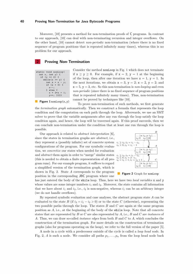
40 Proving Non-Termination for Java Bytecode Programs
Moreover, [10] presents a method for non-termination proofs of C programs. In contrastto our approach, [10] can deal with non-terminating recursion and integer overflows. Onthe other hand, [10] cannot detect non-periodic non-termination (where there is no fixedsequence of program positions that is repeated infinitely many times), whereas this is noproblem for our approach.
2 Proving Non-Termination
static void nonLoop (int x, int y)
if (y >= 0) while (x >= y)
int z = x - y;if (z > 0)
x--; else
x = 2*x + 1;y++;
Figure 1 nonLoop(x,y)
Consider the method nonLoop in Fig. 1 which does not terminateif x ≥ y ≥ 0. For example, if x = 2, y = 1 at the beginningof the loop, then after one iteration we have x = 1, y = 1. Inthe next iterations, we obtain x = 3, y = 2; x = 2, y = 2; andx = 5, y = 3, etc. So this non-termination is non-looping and evennon-periodic (since there is no fixed sequence of program positionsthat is repeated infinitely many times). Thus, non-terminationcannot be proved by techniques like [10].
To prove non-termination of such methods, we first generatethe termination graph automatically. Then we construct a formula that represents the loopcondition and the computation on each path through the loop. Afterwards, we use an SMTsolver to prove that the variable assignments after any run through the loop satisfy the loopcondition again, and hence, the loop will be traversed again. If this proof succeeds, then wecan conclude non-termination under the condition that at least one run through the loop ispossible.
. . . |x : i4, y : i2 | . . .i4:Z i2: [≥0]
B
. . . |x : i1, y : i2 | . . .i1:Z i2: [≥0]
A
. . . |x : i6, y : i7 | . . .i6:Z i7: [>0]
C
i1 ≥ i2, i3 = i1 − i2,i3 > 0, i4 = i1 − 1
i1 ≥ i2, i3 = i1 − i2,i3 ≤ 0, i5 = 2 · i1,i6 = i5 + 1, i7 = i2 + 1
Figure 2 Graph for nonLoop
Our approach is related to abstract interpretation [6],since the states in termination graphs are abstract, i.e.,they represent a (possibly infinite) set of concrete systemconfigurations of the program. For our symbolic evalua-tion, we concretize our states when needed for evaluationand abstract them again in order to “merge” similar states(this is needed to obtain a finite representation of all pro-gram runs). For our example program, it suffices to regarda simplified version of the termination graph, which isshown in Fig. 2. State A corresponds to the programposition in the corresponding JBC program where onehas just entered the body of the while loop. Thus, here we have two local variables x and y
whose values are some integer numbers i1 and i2. Moreover, the state contains all informationthat we have about i1 and i2, i.e., i2 is non-negative, whereas i1 can be an arbitrary integer(we do not handle overflows).
By repeated symbolic evaluation and case analyses, the abstract program state A can beevaluated to the state B (if i3 = i1 − i2 > 0) or to the state C (otherwise), representing thetwo possible paths through the loop. The states B and C are again at the same programposition as A, i.e., at the beginning of the body of the while loop. Note that all concretestates that are represented by B or C are also represented by A, i.e., B and C are instances ofA. Thus, we can draw so-called instance edges from both B and C to A, which concludes theconstruction of the termination graph. For more details on the construction of terminationgraphs (also for programs operating on the heap), we refer to the full version of the paper [5].
A node in a cycle with a predecessor outside of the cycle is called a loop head node. InFig. 2, A is such a node. We consider all paths p1, . . . , pn from the loop head node back
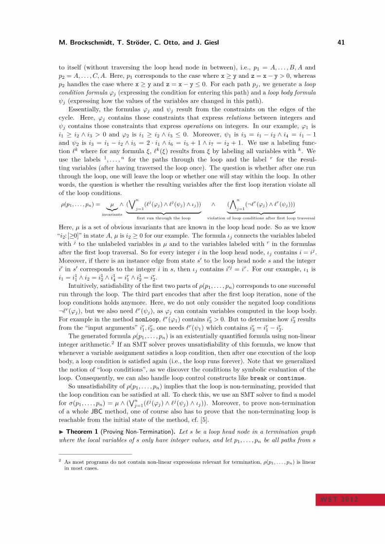
M. Brockschmidt, T. Ströder, C. Otto, and J. Giesl 41
to itself (without traversing the loop head node in between), i.e., p1 = A, . . . , B,A andp2 = A, . . . , C,A. Here, p1 corresponds to the case where x ≥ y and z = x− y > 0, whereasp2 handles the case where x ≥ y and z = x− y ≤ 0. For each path pj , we generate a loop
condition formula ϕj (expressing the condition for entering this path) and a loop body formula
ψj (expressing how the values of the variables are changed in this path).Essentially, the formulas ϕj and ψj result from the constraints on the edges of the
cycle. Here, ϕj contains those constraints that express relations between integers andψj contains those constraints that express operations on integers. In our example, ϕ1 isi1 ≥ i2 ∧ i3 > 0 and ϕ2 is i1 ≥ i2 ∧ i3 ≤ 0. Moreover, ψ1 is i3 = i1 − i2 ∧ i4 = i1 − 1and ψ2 is i3 = i1 − i2 ∧ i5 = 2 · i1 ∧ i6 = i5 + 1 ∧ i7 = i2 + 1. We use a labeling func-tion ℓk where for any formula ξ, ℓk(ξ) results from ξ by labeling all variables with k. Weuse the labels 1, . . . , n for the paths through the loop and the label r for the resul-ting variables (after having traversed the loop once). The question is whether after one runthrough the loop, one will leave the loop or whether one will stay within the loop. In otherwords, the question is whether the resulting variables after the first loop iteration violate allof the loop conditions.
ρ(p1, . . . , pn) = µ︸︷︷︸
invariants
∧ (∨n
j=1(ℓj(ϕj) ∧ ℓ
j(ψj) ∧ ιj))
︸ ︷︷ ︸
first run through the loop
∧ (∧n
j=1(¬ℓr(ϕj) ∧ ℓ
r(ψj)))
︸ ︷︷ ︸
violation of loop conditions after first loop traversal
Here, µ is a set of obvious invariants that are known in the loop head node. So as we know“i2: [≥0]” in state A, µ is i2 ≥ 0 for our example. The formula ιj connects the variables labeledwith j to the unlabeled variables in µ and to the variables labeled with r in the formulasafter the first loop traversal. So for every integer i in the loop head node, ιj contains i = ij .Moreover, if there is an instance edge from state s′ to the loop head node s and the integeri′ in s′ corresponds to the integer i in s, then ιj contains i′j = ir. For our example, ι1 isi1 = i11 ∧ i2 = i12 ∧ i
14 = ir1 ∧ i
12 = ir2.
Intuitively, satisfiability of the first two parts of ρ(p1, . . . , pn) corresponds to one successfulrun through the loop. The third part encodes that after the first loop iteration, none of theloop conditions holds anymore. Here, we do not only consider the negated loop conditions¬ℓr(ϕj), but we also need ℓr(ψj), as ϕj can contain variables computed in the loop body.For example in the method nonLoop, ℓr(ϕ1) contains ir3 > 0. But to determine how ir3 resultsfrom the “input arguments” ir1, i
r2, one needs ℓr(ψ1) which contains ir3 = ir1 − i
r2.
The generated formula ρ(p1, . . . , pn) is an existentially quantified formula using non-linearinteger arithmetic.2 If an SMT solver proves unsatisfiability of this formula, we know thatwhenever a variable assignment satisfies a loop condition, then after one execution of the loopbody, a loop condition is satisfied again (i.e., the loop runs forever). Note that we generalizedthe notion of “loop conditions”, as we discover the conditions by symbolic evaluation of theloop. Consequently, we can also handle loop control constructs like break or continue.
So unsatisfiability of ρ(p1, . . . , pn) implies that the loop is non-terminating, provided thatthe loop condition can be satisfied at all. To check this, we use an SMT solver to find a modelfor σ(p1, . . . , pn) = µ ∧ (
∨nj=1(ℓj(ϕj) ∧ ℓj(ψj) ∧ ιj)). Moreover, to prove non-termination
of a whole JBC method, one of course also has to prove that the non-terminating loop isreachable from the initial state of the method, cf. [5].
Theorem 1 (Proving Non-Termination). Let s be a loop head node in a termination graph
where the local variables of s only have integer values, and let p1, . . . , pn be all paths from s
2 As most programs do not contain non-linear expressions relevant for termination, ρ(p1, . . . , pn) is linearin most cases.
WST 2012
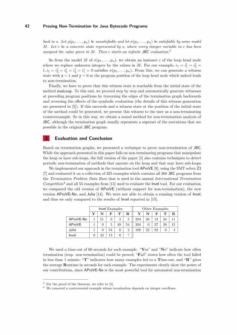
42 Proving Non-Termination for Java Bytecode Programs
back to s. Let ρ(p1, . . . , pn) be unsatisfiable and let σ(p1, . . . , pn) be satisfiable by some model
M . Let c be a concrete state represented by s, where every integer variable in c has been
assigned the value given in M . Then c starts an infinite JBC evaluation.3
So from the model M of σ(p1, . . . , pn), we obtain an instance c of the loop head nodewhere we replace unknown integers by the values in M . For our example, i1 = i11 = i13 =1, i2 = i12 = ir2 = i14 = ir1 = 0 satisfies σ(p1, . . . , pn). From this, we can generate a witnessstate with x = 1 and y = 0 at the program position of the loop head node which indeed leadsto non-termination.
Finally, we have to prove that this witness state is reachable from the initial state of themethod nonLoop. To this end, we proceed step by step and automatically generate witnessesat preceding program positions by traversing the edges of the termination graph backwardsand reversing the effects of the symbolic evaluation (the details of this witness generationare presented in [5]). If this succeeds and a witness state at the position of the initial stateof the method could be generated, we present this witness to the user as a non-terminatingcounterexample. So in this way, we obtain a sound method for non-termination analysis ofJBC, although the termination graph usually represents a superset of the executions that arepossible in the original JBC program.
3 Evaluation and Conclusion
Based on termination graphs, we presented a technique to prove non-termination of JBC.While the approach presented in this paper fails on non-terminating programs that manipulatethe heap or have sub-loops, the full version of the paper [5] also contains techniques to detectperiodic non-termination of methods that operate on the heap and that may have sub-loops.
We implemented our approach in the termination tool AProVE [9], using the SMT solver Z3
[7] and evaluated it on a collection of 325 examples which contains all 268 JBC programs fromthe Termination Problem Data Base that is used in the annual International Termination
Competition4 and all 55 examples from [15] used to evaluate the Invel tool. For our evaluation,we compared the old version of AProVE (without support for non-termination), the newversion AProVE-No, and Julia [14]. We were not able to obtain a running version of Invel,and thus we only compared to the results of Invel reported in [15].
Invel Examples Other Examples
Y N F T R Y N F T R
AProVE-No 1 51 0 3 5 204 30 12 24 11
AProVE 1 0 5 49 54 204 0 27 39 15
Julia 1 0 54 0 2 166 22 82 0 4
Invel 0 42 13 0 ?
We used a time-out of 60 seconds for each example. “Yes” and “No” indicate how oftentermination (resp. non-termination) could be proved, “Fail” states how often the tool failedin less than 1 minute, “T” indicates how many examples led to a Time-out, and “R” givesthe average Runtime in seconds for each example. The experiments clearly show the power ofour contributions, since AProVE-No is the most powerful tool for automated non-termination
3 For the proof of the theorem, we refer to [5].4 We removed a controversial example whose termination depends on integer overflows.
M. Brockschmidt, T. Ströder, C. Otto, and J. Giesl 43
proofs of Java resp. JBC programs. Moreover, the comparison between AProVE-No andAProVE indicates that the runtime for termination proofs did not increase due to the addednon-termination techniques. To experiment with our implementation via a web interface andfor further details, we refer to [1] and to the full version of the paper [5].
References
1 http://aprove.informatik.rwth-aachen.de/eval/JBC-Nonterm/.2 B. Beckert, R. Hähnle, and P. H. Schmitt. Verification of Object-Oriented Software: The
KeY Approach. LNCS 4334. 2007.3 M. Brockschmidt, C. Otto, C. von Essen, and J. Giesl. Termination graphs for Java
Bytecode. In Verification, Induction, Termination Analysis, LNCS 6463, pages 17–37, 2010.Extended version (with proofs) available at [1].
4 M. Brockschmidt, C. Otto, and J. Giesl. Modular termination proofs of recursive Java
Bytecode programs by term rewriting. In Proc. RTA ’11, LIPIcs 10, pages 155–170, 2011.Extended version (with proofs) available at [1].
5 M. Brockschmidt, T. Ströder, C. Otto, and J. Giesl. Automated detection of non-termination and NullPointerExceptions for Java Bytecode. In Proc. FoVeOOS ’11, LNCS.To appear. Extended version (with proofs) appeared as Technical Report AIB 2011-17,RWTH Aachen, 2011. Available at [1] and at aib.informatik.rwth-aachen.de.
6 P. Cousot and R. Cousot. Abstract interpretation: A unified lattice model for staticanalysis of programs by construction or approximation of fixpoints. In Proc. POPL ’77,pages 238–252. ACM Press, 1977.
7 L. de Moura and N. Bjørner. Z3: An efficient SMT solver. In Proc. TACAS ’08, LNCS4963, pages 337–340, 2008.
8 J. Giesl, R. Thiemann, and P. Schneider-Kamp. Proving and disproving termination ofhigher-order functions. In Proc. FroCoS ’05, LNAI 3717, pages 216–231, 2005.
9 J. Giesl, P. Schneider-Kamp, and R. Thiemann. AProVE 1.2: Automatic termination proofsin the dependency pair framework. In Proc. IJCAR ’06, LNAI 4130, pages 281–286, 2006.
10 A. Gupta, T. A. Henzinger, R. Majumdar, A. Rybalchenko, and R. Xu. Proving non-termination. In Proc. POPL ’08, pages 147–158. ACM Press, 2008.
11 C. Otto, M. Brockschmidt, C. von Essen, and J. Giesl. Automated termination analysisof Java Bytecode by term rewriting. In Proc. RTA ’10, LIPIcs 6, pages 259–276, 2010.Extended version (with proofs) available at [1].
12 É. Payet and F. Mesnard. Nontermination inference of logic programs. ACM Trans. Prog.
Lang. Syst., 28:256–289, 2006.13 É. Payet. Loop detection in term rewriting using the eliminating unfoldings. Theoretical
Computer Science, 403:307–327, 2008.14 É. Payet and F. Spoto. Experiments with non-termination analysis for Java Bytecode. In
Proc. BYTECODE ’09, ENTCS 5, pages 83–96, 2009.15 H. Velroyen and P. Rümmer. Non-termination checking for imperative programs. In Proc.
TAP ’08, LNCS 5051, pages 154–170, 2008.
WST 2012
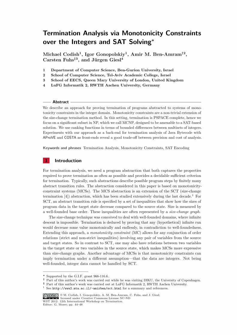
Termination Analysis via Monotonicity Constraints
over the Integers and SAT Solving∗
Michael Codish1, Igor Gonopolskiy1, Amir M. Ben-Amram†2,
Carsten Fuhs‡3, and Jürgen Giesl4
1 Department of Computer Science, Ben-Gurion University, Israel
2 School of Computer Science, Tel-Aviv Academic College, Israel
3 School of EECS, Queen Mary University of London, United Kingdom
4 LuFG Informatik 2, RWTH Aachen University, Germany
Abstract
We describe an approach for proving termination of programs abstracted to systems of mono-
tonicity constraints in the integer domain. Monotonicity constraints are a non-trivial extension of
the size-change termination method. In this setting, termination is PSPACE complete, hence we
focus on a significant subset in NP, which we call MCNP, designed to be amenable to a SAT-based
solution. We use ranking functions in terms of bounded differences between multisets of integers.
Experiments with our approach as a back-end for termination analysis of Java Bytecode with
AProVE and COSTA as front-ends reveal a good trade-off between precision and cost of analysis.
Keywords and phrases Termination Analysis, Monotonicity Constraints, SAT Encoding
1 Introduction
For termination analysis, we need a program abstraction that both captures the properties
required to prove termination as often as possible and provides a decidable sufficient criterion
for termination. Typically, such abstractions describe possible program steps by finitely many
abstract transition rules. The abstraction considered in this paper is based on monotonicity-
constraint systems (MCSs). The MCS abstraction is an extension of the SCT (size-change
termination [4]) abstraction, which has been studied extensively during the last decade.1 For
SCT, an abstract transition rule is specified by a set of inequalities that show how the sizes of
program data in the target state decrease compared to the source state. Size is measured by
a well-founded base order. These inequalities are often represented by a size-change graph.
The size-change technique was conceived to deal with well-founded domains, where infinite
descent is impossible. Termination is deduced by proving that any (hypothetical) infinite run
would decrease some value monotonically and endlessly, in contradiction to well-foundedness.
Extending this approach, a monotonicity constraint (MC) allows for any conjunction of order
relations (strict and non-strict inequalities) involving any pair of variables from the source
and target states. So in contrast to SCT, one may also have relations between two variables
in the target state or two variables in the source state, which makes MCSs more expressive
than size-change graphs. Another advantage of MCSs is that monotonicity constraints can
imply termination under a different assumption—that the data are integers. Not being
well-founded, integer data cannot be handled by SCT.
∗ Supported by the G.I.F. grant 966-116.6.† Part of this author’s work was carried out while he was visiting DIKU, the University of Copenhagen.‡ Part of this author’s work was carried out at LuFG Informatik 2, RWTH Aachen University.1 See http://www2.mta.ac.il/~amirben/sct.html for a summary and references.
© M. Codish, I. Gonopolskiy, A. M. Ben-Amram, C. Fuhs, and J. Giesl;licensed under Creative Commons License NC-ND
WST 2012: 12th International Workshop on Termination.Editor: G. Moser; pp. 44–48
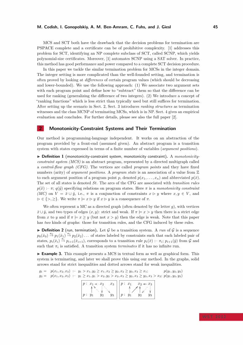
M. Codish, I. Gonopolskiy, A. M. Ben-Amram, C. Fuhs, and J. Giesl 45
MCS and SCT both have the drawback that the decision problems for termination are
PSPACE complete and a certificate can be of prohibitive complexity. [1] addresses this
problem for SCT, identifying an NP complete subclass of SCT, called SCNP, which yields
polynomial-size certificates. Moreover, [1] automates SCNP using a SAT solver. In practice,
this method has good performance and power compared to a complete SCT decision procedure.
In this paper we tackle the similar termination problem for MCSs in the integer domain.
The integer setting is more complicated than the well-founded setting, and termination is
often proved by looking at differences of certain program values (which should be decreasing
and lower-bounded). We use the following approach: (1) We associate two argument sets
with each program point and define how to “subtract” them so that the difference can be
used for ranking (generalizing the difference of two integers). (2) We introduce a concept of
“ranking functions” which is less strict than typically used but still suffices for termination.
After setting up the scenario in Sect. 2, Sect. 3 introduces ranking structures as termination
witnesses and the class MCNP of terminating MCSs, which is in NP. Sect. 4 gives an empirical
evaluation and concludes. For further details, please see also the full paper [2].
2 Monotonicity-Constraint Systems and Their Termination
Our method is programming-language independent. It works on an abstraction of the
program provided by a front-end (assumed given). An abstract program is a transition
system with states expressed in terms of a finite number of variables (argument positions).
Definition 1 (monotonicity-constraint system, monotonicity constraint). A monotonicity-
constraint system (MCS) is an abstract program, represented by a directed multigraph called
a control-flow graph (CFG). The vertices are called program points and they have fixed
numbers (arity) of argument positions. A program state is an association of a value from Z
to each argument position of a program point p, denoted p(x1, . . . , xn) and abbreviated p(x).
The set of all states is denoted St. The arcs of the CFG are associated with transition rules
p(x) :– π; q(y) specifying relations on program states. Here π is a monotonicity constraint
(MC) on V = x ∪ y, i.e., π is a conjunction of constraints x ⊲ y where x, y ∈ V , and
⊲ ∈ >,≥. We write π |= x⊲ y if x⊲ y is a consequence of π.
We often represent a MC as a directed graph (often denoted by the letter g), with vertices
x∪ y, and two types of edges (x, y): strict and weak. If π |= x > y then there is a strict edge
from x to y and if π |= x ≥ y (but not x > y) then the edge is weak. Note that this paper
has two kinds of graphs: those for transition rules, and the CFG induced by these rules.
Definition 2 (run, termination). Let G be a transition system. A run of G is a sequence
p0(x0)π0→ p1(x1)
π1→ p2(x2) . . . of states labeled by constraints such that each labeled pair of
states, pi(xi)πi→ pi+1(xi+1), corresponds to a transition rule pi(x) :– πi; pi+1(y) from G and
such that πi is satisfied. A transition system terminates if it has no infinite run.
Example 3. This example presents a MCS in textual form as well as graphical form. This
system is terminating, and later we shall prove this using our method. In the graphs, solid
arrows stand for strict inequalities and dotted arrows stand for weak inequalities.
g1 = p(x1, x2, x3) :– y1 > x1, y2 ≥ x1, x2 ≥ y2, x2 ≥ y3, x2 ≥ x1; p(y1, y2, y3)
g2 = p(x1, x2, x3) :– y1 ≥ x1, y1 > x2, y2 > x2, x3 ≥ y2, x3 ≥ y3, x3 > x2; p(y1, y2, y3)
p :
p :
x1 x2oo
x3
y1
OO
y2
^^
y3
p :
p :
x1 x2 x3oo
y1
OO @@
y2
OO
y3
WST 2012
46 Termination Analysis via Monotonicity Constraints over the Integers and SAT Solving
3 Ranking Structures for MCSs and MCNP
For a quasi-order %, its strict part x ≻ y is (x % y) ∧ (y 6% x), and it is well-founded if there
is no infinite ≻-chain. A set is well-founded if it has a tacitly-understood well-founded order.
A ranking function maps program states into a well-founded set, such that every transition
decreases the function’s value. Generalizing, we introduce ranking structures, which are more
flexible than ranking functions, and suffice for most practical termination proofs.
Definition 4 (anchor, intermittent ranking function). Let G be a MCS with state space
St. Let (D,%) be a quasi-order and D+ a well-founded subset of D. Consider a function
Φ : St→ D. We say that g ∈ G is a Φ-anchor for G (or that g is anchored by Φ for G) if for
every run p0(x0)π0→ p1(x1)
π1→ . . .πk−1
→ pk(xk)πk→ pk+1(xk+1) where both p0(x0)
π0→ p1(x1) and
pk(xk)πk→ pk+1(xk+1) correspond to the transition rule g, we have Φ(pi(xi)) % Φ(pi+1(xi+1))
for all 0 ≤ i ≤ k, where at least one of these inequalities is strict; and Φ(pi(xi)) ∈ D+ for
some 0 ≤ i ≤ k. Such a function Φ is called an intermittent ranking function (IRF).
Example 5. Consider the transition rules from Ex. 3 inducing the MCS G. Let Φ1(p(x)) =
max(x2, x3)− x1. In any run built with g1 and g2, the value of Φ1 is non-negative at least in
every state followed by a transition by g1. Moreover, a transition by g1 decreases the value
strictly and a transition by g2 decreases it weakly. Hence, g1 is anchored by Φ1 for G.
Definition 6 (ranking structure). Consider G and D as in Def. 4. Let Φ1, . . . ,Φm : St→ D.
Let G1 consist of all transition rules g ∈ G where Φ1 anchors g for G. For 2 ≤ i ≤ m, let Giconsist of all transition rules g ∈ G\(G1∪ . . .∪Gi−1) where Φi anchors g in G\(G1∪ . . .∪Gi−1).
We say that 〈Φ1, . . . ,Φm〉 is a ranking structure for G if G1 ∪ . . . ∪ Gm = G.
Note that by the above definition, for every g ∈ G there is a (unique) Gi with g ∈ Gi.
Example 7. For the program of Ex. 3, a ranking structure is 〈Φ1,Φ2〉 with Φ1 as in Ex. 5
and Φ2(p(x)) = x3 − x2. Here, we have g1 ∈ G1 and g2 ∈ G2.
Theorem 8. If there is a ranking structure for G, then G terminates.
The building blocks for our construction are two2 quasi-orders on multisets of integers
and a notion of level mappings from program states into pairs of multisets, whose difference
(not set-theoretic difference; see Def. 13 below) will be used to rank the states. The difference
will be itself a multiset, and we use the following relations to order such multisets.
Definition 9 (multiset types). Let ℘n(Z) denote the set of multisets of integers of at most
n elements, where n is fixed by context.3 The µ-ordered multiset type, for µ ∈ max,min ,
is the quasi-ordered set (℘n(Z),%µ) where:
1. (max order) S %max T holds iff max(S) ≥ max(T ), or T is empty; S ≻max T holds iff
max(S) > max(T ), or T is empty while S is not.
2. (min order) S %min T holds iff min(S) ≥ min(T ), or S is empty; S ≻min T holds iff
min(S) > min(T ), or S is empty while T is not.
Example 10. For S = 10, 8, 5, T = 9, 5: S ≻max T , T %min S.
Definition 11 (well-founded subset of multiset types). For µ ∈ max,min , we define
(℘n(Z),%µ)+ as follows: For min (respectively max) order, the subset consists of the multisets
whose minimum (resp. maximum) is non-negative.
Lemma 12. For all µ ∈ max,min , (℘n(Z),%µ) is a total quasi-order, with ≻µ its
strict part; and (℘n(Z),%µ)+ is well-founded.
2 The full version of this paper [2] additionally uses the multiset order and the dual multiset order.3 For monotonicity-constraint systems, n is the maximum arity of program points.
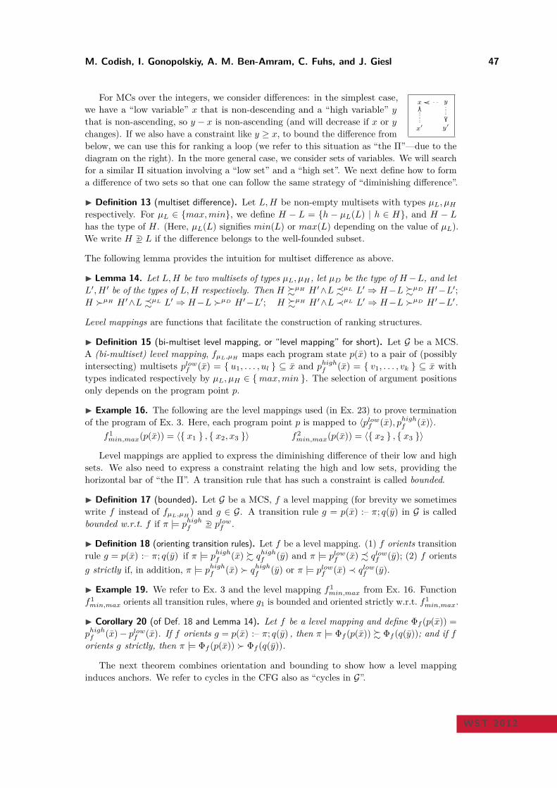
M. Codish, I. Gonopolskiy, A. M. Ben-Amram, C. Fuhs, and J. Giesl 47
x yoo
x′
OO
y′
For MCs over the integers, we consider differences: in the simplest case,
we have a “low variable” x that is non-descending and a “high variable” y
that is non-ascending, so y − x is non-ascending (and will decrease if x or y
changes). If we also have a constraint like y ≥ x, to bound the difference from
below, we can use this for ranking a loop (we refer to this situation as “the Π”—due to the
diagram on the right). In the more general case, we consider sets of variables. We will search
for a similar Π situation involving a “low set” and a “high set”. We next define how to form
a difference of two sets so that one can follow the same strategy of “diminishing difference”.
Definition 13 (multiset difference). Let L,H be non-empty multisets with types µL, µHrespectively. For µL ∈ max,min, we define H − L = h − µL(L) | h ∈ H, and H − L
has the type of H. (Here, µL(L) signifies min(L) or max(L) depending on the value of µL).
We write H G L if the difference belongs to the well-founded subset.
The following lemma provides the intuition for multiset difference as above.
Lemma 14. Let L,H be two multisets of types µL, µH , let µD be the type of H−L, and let
L′, H ′ be of the types of L,H respectively. Then H %µH H ′∧L -µL L′ ⇒ H−L %µD H ′−L′;
H ≻µH H ′∧L -µL L′ ⇒ H−L ≻µD H ′−L′; H %µH H ′∧L ≺µL L′ ⇒ H−L ≻µD H ′−L′.
Level mappings are functions that facilitate the construction of ranking structures.
Definition 15 (bi-multiset level mapping, or “level mapping” for short). Let G be a MCS.
A (bi-multiset) level mapping, fµL,µH maps each program state p(x) to a pair of (possibly
intersecting) multisets plowf (x) = u1, . . . , ul ⊆ x and phighf (x) = v1, . . . , vk ⊆ x with
types indicated respectively by µL, µH ∈ max,min . The selection of argument positions
only depends on the program point p.
Example 16. The following are the level mappings used (in Ex. 23) to prove termination
of the program of Ex. 3. Here, each program point p is mapped to 〈plowf (x), phighf (x)〉.
f1min,max(p(x)) = 〈 x1 , x2, x3 〉 f2
min,max(p(x)) = 〈 x2 , x3 〉
Level mappings are applied to express the diminishing difference of their low and high
sets. We also need to express a constraint relating the high and low sets, providing the
horizontal bar of “the Π”. A transition rule that has such a constraint is called bounded.
Definition 17 (bounded). Let G be a MCS, f a level mapping (for brevity we sometimes
write f instead of fµL,µH ) and g ∈ G. A transition rule g = p(x) :– π; q(y) in G is called
bounded w.r.t. f if π |= phighf G plowf .
Definition 18 (orienting transition rules). Let f be a level mapping. (1) f orients transition
rule g = p(x) :– π; q(y) if π |= phighf (x) % qhighf (y) and π |= plowf (x) - qlowf (y); (2) f orients
g strictly if, in addition, π |= phighf (x) ≻ qhighf (y) or π |= plowf (x) ≺ qlowf (y).
Example 19. We refer to Ex. 3 and the level mapping f1min,max from Ex. 16. Function
f1min,max orients all transition rules, where g1 is bounded and oriented strictly w.r.t. f1
min,max.
Corollary 20 (of Def. 18 and Lemma 14). Let f be a level mapping and define Φf (p(x)) =
phighf (x)− plowf (x). If f orients g = p(x) :– π; q(y) , then π |= Φf (p(x)) % Φf (q(y)); and if f
orients g strictly, then π |= Φf (p(x)) ≻ Φf (q(y)).
The next theorem combines orientation and bounding to show how a level mapping
induces anchors. We refer to cycles in the CFG also as “cycles in G”.
WST 2012
48 Termination Analysis via Monotonicity Constraints over the Integers and SAT Solving
Theorem 21. Let G be a MCS and f a level mapping. Let g = p(x) :– π; q(y) be such
that every cycle C including g satisfies these conditions: (1) all transitions in C are oriented
by f , and at least one of them strictly; (2) at least one transition in C is bounded w.r.t. f .
Then g is a Φf -anchor for G, where Φf (p(x)) = phighf (x)− plowf (x).
Definition 22 (MCNP anchors and ranking functions). Let G be a MCS and f a level
mapping. We say that g is a MCNP-anchor for G w.r.t. f if f and g satisfy the conditions of
Thm. 21. Φf is called a MCNP (intermittent) ranking function (MCNP IRF). A system of
monotonicity constraints is in MCNP if it has a tuple of MCNP IRFs as a ranking structure.
It follows from Thm. 8 that if a MCS is in MCNP, then it terminates.
Example 23. Consider again Ex. 3 and Ex. 16. Then, 〈Φf1 ,Φf2〉 is a ranking structure
for G. The facts in Ex. 19 imply that g1 is an MCNP-anchor w.r.t. f1. Moreover, f2 is both
strict and bounded on g2.
One can now show that MCNP is in NP. Thus, for automation we use a SAT encoding to
find termination proofs using an off-the-shelf SAT solver. We invoke a SAT solver iteratively
to generate level-mappings and construct a ranking structure 〈Φ1,Φ2, . . . ,Φm〉. Details on
the algorithm and on the encoding can be found in the full version of this paper [2].
4 Experiments and Conclusion
We implemented a termination analyzer based on our SAT encoding for MCNP and tested
it on several benchmark suites. For details on our experiments please see http://aprove.
informatik.rwth-aachen.de/eval/MCNP. As part of our experiments, we applied our
MCNP implementation on MCS abstractions of over 100 Java Bytecode programs which
were obtained using the termination tools AProVE and COSTA. Our results show that MCNP
is almost as powerful as the back-ends of AProVE and COSTA, and its performance is
competitive, especially in comparison to the rewrite-based tool AProVE. Thus, it could
be fruitful to use a combination of tools where the MCNP-analyzer is tried first and the
rewrite-based analyzer is only applied for the remaining “hard” examples.
To conclude, we introduced a new approach to prove termination of monotonicity-
constraint transition systems. The idea is to construct a ranking structure, of a novel kind,
extending previous work in this area. For automation, we use a SAT-based approach, which
we evaluated in extensive experiments. The results demonstrate the power of our approach
and show that its integration into termination tools for Java Bytecode advances the state of
the art of automated termination analysis. The full version of this paper has appeared in [2].
Acknowledgment. We thank Samir Genaim for help with the benchmarking.
References
1 A. M. Ben-Amram and M. Codish. A SAT-based approach to size-change termination with
global ranking functions. In Proc. TACAS ’08, LNCS 4963, pp. 218–232, 2008.
2 M. Codish, I. Gonopolskiy, A. M. Ben-Amram, C. Fuhs, J. Giesl. SAT-based termination
analysis using monotonicity constraints over the integers. In Proc. ICLP ’11, Theory and
Practice of Logic Programming, 11(4–5), 503–520, 2011.
3 M. Codish, V. Lagoon, and P. J. Stuckey. Testing for termination with monotonicity
constraints. In Proc. ICLP ’05, LNCS 3668, pp. 326–340, 2005.
4 C. S. Lee, N. D. Jones, and A. M. Ben-Amram. The size-change principle for program
termination. In Proc. POPL ’01, ACM Press, pp. 81–92, 2001.
Detecting Non-Looping Non-Termination∗
Fabian Emmes, Tim Enger, and Jürgen Giesl
LuFG Informatik 2, RWTH Aachen University, Germany
Abstract
We introduce a technique to prove non-termination of term rewrite systems automatically. Incontrast to most previous approaches, our technique is also able to detect non-looping non-termination.
1998 ACM Subject Classification D.2.4 - Software/Program Verification, F.3.1 - Specifyingand Verifying and Reasoning about Programs, F.4.2 - Grammars and Other Rewriting Systems,I.2.2 - Automatic Programming
Keywords and phrases Non-termination, Loops, Term Rewriting
1 Introduction
To prove constructively that a term rewrite system (TRS) is non-terminating, one has toprovide a finite description of how to obtain an infinite rewrite sequence. The most commonway to do so is in the form of loops. A loop is a finite sequence of rewrite steps, such thatthe start term of the sequence is embedded in the final term.
Definition 1 (Loops). A TRS R is called looping, if there is a term u, a context C, and asubstitution µ such that u→+
RC[uµ].
Since term rewriting is closed under substitutions and contexts, from any loop it ispossible to construct an infinite rewrite sequence u→n
RC[uµ]→n
RC[Cµ[uµ2]]→n
R. . . for
some n > 0.To detect loops automatically, one can start with a rule and then repeatedly narrow
it using other rules (see e.g. [3, 4, 10, 12, 14, 15] for existing work on proving loopingnon-termination of TRSs). Narrowing is similar to rewriting, but instead of matching theleft-hand side of a rule with a subterm, one uses unification. In this way, one constructslonger and longer rewrite sequences u→+
Rv. As soon as u semi-unifies with a subterm v|π
of v (i.e., uδ1δ2 = v|πδ1 for some substitutions δ1 and δ2), one has found a loop, since
uδ1 →+Rvδ1 = vδ1[v|πδ1]π = vδ1[uδ1δ2]π.
This approach is suitable for automation, since semi-unification is decidable and algorithmsfor semi-unification were presented in [6, 8], for example.
2 Non-Looping Non-Termination
While interesting classes and examples of non-looping TRSs were identified in earlier papers(e.g., [2, 13]), up to now virtually all methods to prove non-termination of TRSs automatically
∗ Supported by the DFG grant GI 274/5-3
© F. Emmes, T. Enger, and J. Giesl;
licensed under Creative Commons License NC-ND
WST 2012: 12th International Workshop on Termination.
Editor: G. Moser; pp. 49–53
50 Detecting Non-Looping Non-Termination
were restricted to looping non-termination.1 A notable exception, although restricted tostring rewrite systems (SRSs), is a technique and tool for non-termination proofs of non-looping SRSs given in [9]. This approach uses an abstract rewrite relation, where rules arenot pairs of strings, but pairs of patterns of the form uvnw. Here, u, v, and w are stringsand n can be instantiated by a natural number.
Our goal is to extend this idea in order to obtain a powerful automated technique fornon-termination of (possibly non-looping) term rewrite systems.
Example 2. Let R be the TRS consisting of the following rules:
isNat(0) → true (1)
isNat(s(x)) → isNat(x) (2)
f(true, x) → f(isNat(x), s(x)) (3)
This system is non-terminating, but not looping. To see this, note that any infiniterewrite sequence has the following form (up to contexts):
f(true, sn(0)) →R f(isNat(sn(0)), sn+1(0))→n+1R
f(true, sn+1(0))
→R f(isNat(sn+1(0)), sn+2(0))→n+2R
f(true, sn+2(0))
. . .
Since the number of steps required to reduce the isNat-terms to true increases in everyiteration, this sequence cannot be represented as a loop. In other words, loops cannot capturenon-periodic infinite rewrite sequences.
To represent such sequences, we extend the idea of [9] from strings to terms and defineso-called pattern rules which are parameterized over the natural numbers. Instantiating theparameter results in a pair of terms u, v such that u→+
Rv. This allows us to capture certain
rewrite sequences of arbitrary length by a finite representation.For instance, the effect of repeated application of rule (2) on the same position can be
captured by the pattern rule
isNat(x)[x/s(x)]n → isNat(x) (4)
with the parameter n, where [x/s(x)]n means that the substitution [x/s(x)] is applied ntimes. Then, for every natural number n, the term pair resulting from the instantiation iscontained in →n
R(i.e., isNat(sn(x))→n
RisNat(x)).
To prove non-termination, we now proceed in a similar way as in existing techniquesto find loops. More precisely, we extend the concept of narrowing from ordinary rules topattern rules. In this way, we can generate new pattern rules that describe longer and longerrewrite sequences. Finally, we use a variant of semi-unification to check whether one of thenewly obtained pattern rules directly leads to non-termination.
1 For automated non-termination proofs of programs, the situation is similar, i.e., most of the existingautomated approaches for non-termination also just detect loops. However for Java Bytecode, werecently presented an approach that can also detect certain forms of non-looping and non-periodicnon-termination automatically, based on SMT solving [1]. But an adaption of that approach to termrewriting does not seem to be promising, since [1] can only handle non-periodic non-termination incases where there are no sub-loops and where non-termination is due to operations on integers. Thus,this approach is not suitable for TRSs where one treats terms instead of integers and where sub-loops(i.e., recursively defined auxiliary functions like isNat) are common.
F. Emmes, T. Enger, and J. Giesl 51
To illustrate the narrowing of pattern rules, we first narrow the pattern rule (4) with rule(1). In other words, the variable x in the pattern rule is instantiated by the term 0, and thenthe resulting right-hand side isNat(0) is rewritten using (1). This yields the new pattern rule
isNat(x)[x/s(x)]n[x/0] → true. (5)
While we narrowed a pattern rule with an ordinary rule above, it is also possible to dothe converse, i.e., one can narrow an ordinary rule with a pattern rule. To see this, we nownarrow rule (3) with the pattern rule (5) which yields
f(true, x)[x/s(x)]n[x/0] → f(true, s(x))[x/s(x)]n[x/0]. (6)
Moreover, one can even narrow pattern rules with pattern rules.The following theorem extends the semi-unification criterion to pattern rules, in order
to detect whether a pattern rule directly leads to non-termination. For a pattern ruleuσnµ → vσnµ, we do not only check whether the base term u on the left-hand side semi-unifies with the base term v on the right-hand side. In addition, one may also apply thepattern substitution σ arbitrary many times to u before performing the semi-unification.
Theorem 3 (Detecting Non-Termination of Pattern Rules). Let uσnµ →+Rvσnµ for all
natural numbers n. If there are a position π of v, a natural number k ∈ N, and two
substitutions δ1 and δ2 such that uσkδ1δ2 = v|πδ1 and such that both δ1 and δ2 commute2
with both σ and µ, then R is non-terminating.
Proof. We show that for all natural numbers n, the term uσnµδ1 rewrites to a term containinga subterm that is an instance of uσk+nµδ1. By repeating these rewrite steps on that subterm,we obtain an infinite rewrite sequence. Here, we denote the superterm relation by D.
uσnµδ1→+Rvσnµδ1 by rewriting
= vδ1σnµ since δ1 commutes with both σ and µ
D uσkδ1δ2σnµ since uσkδ1δ2 = v|πδ1
= uσkδ1σnµδ2 since δ2 commutes with both σ and µ
= uσk+nµδ1δ2 since δ1 commutes with both σ and µ
In our example, the criterion of Thm. 3 can easily detect non-termination of the patternrule (6), i.e., of f(true, x)σnµ → f(true, s(x))σnµ where σ = [x/s(x)] and µ = [x/0]. Letk = 1. Then we have uσk = v, i.e., the term f(true, x)σk is equal to the base term f(true, s(x))of the right-hand side of the pattern rule (6). Thus, we choose δ1 and δ2 to be the identity.Since then δ1 and δ2 trivially commute with σ and µ, non-termination of the original TRSin Ex. 2 follows from Thm. 3.
3 Conclusion
We introduced a new technique to prove non-termination of possibly non-looping TRSsautomatically. The technique extends and subsumes previous approaches to detect loopswhich were based on narrowing and semi-unification. To this end, we adapted an idea of
2 We say that two substitutions δ and σ commute if δσ = σδ.
WST 2012
52 Detecting Non-Looping Non-Termination
[9] from string rewriting to term rewriting and introduced pattern rules which represent awhole class of rewrite sequences. Afterwards, we extended narrowing and semi-unification topattern rules. The technical details and extensions of our approach will be presented in aforthcoming full version of the paper.
We implemented the resulting non-termination prover in the tool AProVE [5] and comparedthe new version AProVE-NL (for non-loop) with the previous version AProVE ’11 and 3 otherpowerful tools for non-termination of TRSs (NTI [10], TTT2 [7], VMTL [11]). We ran thetools on the 1438 TRSs of the Termination Problem Data Base (TPDB) used in the annualInternational Termination Competition.3 In the table, we consider those 241 TRSs of the
TPDB nl
N R N R
AProVE-NL 232 6.6 44 5.2
AProVE ’11 228 6.6 0 60.0
NTI 214 7.3 0 60.0
TTT2 208 9.1 0 60.0
VMTL 95 16.5 0 42.8
TPDB where at least one tool proved non-termination. Moreover, we also tested the toolson a selection of 58 typical non-looping non-terminating TRSs from different sources (“nl”).We used a time-out of 1 minute for each exam-ple. “N” indicates how often Non-termination wasproved and “R” gives the average Runtime in sec-onds for each example. Thus, AProVE-NL couldsolve 75.9 % of the non-looping examples without compromising its power on looping exam-ples, whereas the other tools cannot handle non-looping non-termination. For further detailson the evaluation, we also refer to the forthcoming full version of the paper.
References
1 M. Brockschmidt, T. Ströder, C. Otto, and J. Giesl. Automated detection of non-termination and NullPointerExceptions for Java Bytecode. In Proc. FoVeOOS ’11,LNCS. To appear. Available at http://aprove.informatik.rwth-aachen.de/eval/
JBC-Nonterm and at http://aib.informatik.rwth-aachen.de.2 A. Geser and H. Zantema. Non-looping string rewriting. Informatique Théorique et Appli-
cations, 33(3):279–302, 1999.3 A. Geser, D. Hofbauer, and J. Waldmann. Termination proofs for string rewriting systems
via inverse match-bounds. Journal of Automated Reasoning, 34(4):365–385, 2005.4 J. Giesl, R. Thiemann, and P. Schneider-Kamp. Proving and disproving termination of
higher-order functions. In Proc. FroCoS ’05, LNAI 3717, pages 216–231, 2005.5 J. Giesl, P. Schneider-Kamp, and R. Thiemann. AProVE 1.2: Automatic termination proofs
in the dependency pair framework. In Proc. IJCAR ’06, LNAI 4130, pages 281–286, 2006.6 D. Kapur, D. Musser, P. Narendran, and J. Stillman. Semi-unification. Theoretical Com-
puter Science, 81(2):169–187, 1991.7 M. Korp, C. Sternagel, H. Zankl, and A. Middeldorp. Tyrolean Termination Tool 2. In Proc.
RTA ’09, LNCS 5595, pages 295–304, 2009.8 A. Oliart and W. Snyder. A fast algorithm for uniform semi-unification. In Proc. CADE ’98,
LNAI 1421, pages 239–253, 1998.9 M. Oppelt. Automatische Erkennung von Ableitungsmustern in nichtterminierenden Wort-
ersetzungssystemen, 2008. Diploma Thesis, HTWK Leipzig, Germany.10 É. Payet. Loop detection in term rewriting using the eliminating unfoldings. Theoretical
Computer Science, 403:307–327, 2008.11 F. Schernhammer and B. Gramlich. VMTL - A modular termination laboratory. In Proc.
RTA ’09, LNCS 5595, pages 285–294, 2009.
3 See http://termination-portal.org/wiki/Termination_Competition
F. Emmes, T. Enger, and J. Giesl 53
12 J. Waldmann. Matchbox: A tool for match-bounded string rewriting. In RTA ’04, LNCS3091, pages 85–94, 2004.
13 Y. Wang and M. Sakai. On non-looping term rewriting. In Proc. WST ’06, pages 17–21,2006.
14 H. Zankl, C. Sternagel, D. Hofbauer, and A. Middeldorp. Finding and certifying loops. InProc. SOFSEM ’10, LNCS 5901, pages 755–766, 2010.
15 H. Zantema. Termination of string rewriting proved automatically. Journal of Automated
Reasoning, 34:105–139, 2005.
WST 2012
Binomial Interpretations∗
Bertram Felgenhauer
Institue of Computer Science, University of Innsbruck, Austria
Abstract
Polynomial interpretations can be used for proving termination of term rewrite systems. In this
note, we contemplate binomial interpretations based on binomial coefficients, and show that they
form a suitable basis for obtaining (weakly) monotone algebras. The main motivation is that
this representation covers examples with negative coefficients like f(x) = 2x2 − x+ 1, and even
some polynomials with rational coefficients like f(x) = x(x− 1)/2 that map natural numbers to
natural numbers.
1 Introduction
Using well-founded monotone algebras is a general and common method for proving termi-
nation of term rewrite systems. Many algebras have been suggested for this purpose. Here
we are mainly interested in polynomial interpretations (introduced by Lankford, [6]). In [8]
it is shown among other things that polynomial interpretations over the real numbers do
not subsume polynomial interpretations over the natural numbers. Ultimately, the reason
for this surprising result lies in the fact that there are polynomials that are non-negative
for every natural number, but negative when evaluated for some real numbers. The exam-
ple f(x) = x(x− 1)/2 shows that there are polynomials with non-integer coefficients that
nevertheless evaluate to integers at every integer argument. Binomial functions (see below)
capture these polynomials precisely.
We are not the first to use binomial functions this way. Girard et al. [1] extend linear
logic with resources bounded by resource polynomials, which are binomial functions with
non-negative coefficients. In more recent work, Hofmann et al. [4, 3] use resource polynomials
for amortized resource analysis of programs. The observation that binomial functions are
closed under composition is much older. The earliest appearances that we are aware of
originate in the study of nilpotent groups [2] and of recursively equivalent sets [7].
In the remainder of the paper, we exhibit some fundamental properties of binomial
coefficients in Section 2, then sketch binomial interpretations in Section 3. In Section 4, we
compare the power of binomial interpretations to standard polynomial interpretations.
2 Fundamentals
Definition 1. For n ∈ N (where N is the set of non-negative integers), and x element of
some ring, the falling power, xn, is defined as follows: (This notation is used by Knuth in [5])
x0 = 1 xn = x · (x− 1)n−1
Falling powers are closely related to binomial coefficients. In fact, we can define binomial
coefficients in terms of falling powers.
Definition 2. For k ∈ N, the binomial coefficient(
xk
)
is defined as(
xk
)
= xk
k! .
∗ This research was supported by the Austrian Science Fund (FWF) project P22467-N23.
© B. Felgenhauer;licensed under Creative Commons License NC-ND
WST 2012: 12th International Workshop on Termination.Editor: G. Moser; pp. 54–58
Bertram Felgenhauer 55
Remark. Over some rings, the fraction xk
k! may not have a value for some x. For example,
in the polynomial ring Z[x],(
x2
)
does not exist. The fraction may also have several values (if
the ring is not torsion-free). But we will only work over Z or R, where this does not happen.
It is clear from the definition that the binomial coefficient(
xk
)
is a polynomial in x of
degree k with rational coefficients. It is well known that(
xk
)
∈ Z whenever x ∈ Z.
Lemma 3. Binomial coefficients satisfy a tremendous number of identities. We exhibit
two of them. (Only (1) is used later, but the second one gives some insight into why binomial
functions are closed under composition.)
(
x+ 1
k + 1
)
−
(
x
k + 1
)
=
(
x
k
)
(1)
(
x+ y
k
)
=
k∑
i=0
(
x
i
)(
y
k − i
)
(2)
3 Binomial Interpretations
Definition 4. A monomial over the variables V is a finite product∏
v∈V ′
(
vkv
)
such that
V ′ ⊆ V and 0 < kv ∈ N. We write 1 if the product is empty and v for(
v1
)
. A binomial function
f over a domain D is a linear combination of monomials, f(v1, . . . , vn) =∑
m∈M am ·m
where am ∈ D andM is a finite set of monomials over the variables V = v1, . . . , vn. We can
evaluate binomial functions in the obvious way, substituting values for the formal variables.
We define a difference operator on binomial functions, justified by the identity (1): We let
∆v(∑
m∈M am ·m)
=∑
m∈M am ·∆vm, where on monomials, ∆v∏
w∈V
(
wkw
)
= 0 if v /∈ V
or kv = 0. Otherwise, ∆v∏
w∈V
(
wkw
)
=(
wk′w
)
where k′v = kv − 1 and k′w = kw for w 6= v. It is
easy to see that f(v1, . . . , vi + 1, . . . , vn)− f(v1, . . . , vi, . . . , vn) = (∆vif)(v1, . . . , vi, . . . , vn)
for all binomial functions f and variables vi.
It is known that binomial functions over N are closed under addition, multiplication and
composition [1]. In practice, the best way to compute the results of these operations appears
to be to use the identity (∆nv(
vk
)
)(0) = δn,k, where δn,k = 1 if n = k and δn,k = 0 otherwise.
Once the degree d of a unary binomial function f(x) is known, one can compute its coefficients
from f(0), f(1), . . . , f(d). This can be extended to multiple variables by treating a binomial
function in V with v ∈ V as a unary function in v with coefficients that are binomial functions
over V \v. The difference operator also plays a crucial role in showing that all integer-valued
(over the integers) polynomials can be expressed by binomial functions, as follows. Let f(v)
be an integer-valued polynomial of degree d > 0. Then (∆vf)(v) = f(v + 1) − f(v) is an
integer-valued polynomial of degree d− 1. The function f can be reconstructed from ∆vf
and f(0), and ultimately from the values fi = (∆ivf)(0) for 0 6 i 6 d, and we have just seen
that these define a binomial function. In fact, f(v) =∑di=0 fi
(
vi
)
.
Definition 5. Let F be a signature where each f ∈ F has an arity ari(f). Furthermore let
V = v1, v2, . . . be a countable set of variables. A binomial F-algebra A over a domain D
assigns to each f ∈ F an interpretation fA that is a binomial function over D with variables
v1, . . . vari(f). A binomial F -algebra induces an F -algebra with carrier D by evaluating the
binomial functions.
To use a binomial F-algebra for proving termination of a TRS R, it has to induce a
well-founded monotone algebra that is compatible with R.
WST 2012
56 Binomial Interpretations
Theorem 6. Let A be a F-algebra over N. Then A is a well-founded monotone algebra,
provided that for all f ∈ F , fA(v1, . . . , vn) =∑
m∈M am ·m implies avi > 1 for 1 6 i 6 n.
Furthermore, for any binomial function f(v1, . . . , vn) =∑
m∈M am · m over N, we have
f(v1, . . . , vn) > 0 for all possible values of vi ∈ N, if, and only if, a1 > 0.
Proof. Note that over N, all binomial functions are weakly monotone and nowhere negative.
The theorem follows easily from that observation.
4 Comparison to Polynomial Interpretations
We will show below that neither polynomial interpretations over R nor over N subsume
binomial interpretations. Note that linear binomial interpretations are identical to linear
polynomial interpretations over the integers—the increased power requires higher degree
polynomials. Using the method by Neurauter and Middeldorp [8], which can force weakly
compatible polynomial interpretations to be linear with non-integer coefficients, it is clear
that binomial interpretations do not subsume polynomial interpretations over Q. On the
other hand, if negative coefficients are allowed, binomial interpretations subsume polynomial
interpretations over N with integer coefficients, by way of the identity
xk =
k∑
i=0
i!
n
i
(
x
i
)
where
ni
denotes Stirling numbers of the second kind, which are non-negative integers. The
same relation allows us to transform polynomial interpretations with non-negative coefficients
to binomial interpretations with non-negative coefficients.
We adapt an example from [8] to show that binomial interpretations are not subsumed
by polynomial interpretations over R or N. Let R be the following TRS.
s(0)→ f(0) (1) s(f(s(x)))→ h(f(x), g(x)) (6)
s2(0)→ f(s(0)) (2) f(g(s(x)))→ g(g(f(s(x)))) (7)
g(x)→ h(x, h(x, x)) (3) h(s2(x), h(x, x))→ g(x) (8)
s(x)→ h(0, x) (4) s(x)→ h(x, 0) (9)
g(s(x))→ s(s(g(x))) (5) h(f(x), s(g(x)))→ f(s(x)) (10)
Theorem 7. Termination of the TRS R can be shown by a binomial interpretation.
Proof. We let [0] = 0, [s](x) = x+1, [f](x) = 3(
x2
)
+x, [g](x) = 3x+1, [h](x, y) = x+y. These
are strictly monotone functions on N. For compatibility with R, we obtain the following
constraints.
1 > 0 (1) 3(
x2
)
+ 4x+ 2 > 3(
x2
)
+ 4x+ 1 (6)
2 > 1 (2) 27(
x2
)
+ 48x+ 22 > 27(
x2
)
+ 36x+ 13 (7)
3x+ 1 > 3x (3) 3x+ 2 > 3x+ 1 (8)
x+ 1 > x (4) x+ 1 > x (9)
3x+ 4 > 3x+ 3 (5) 3(
x2
)
+ 4x+ 2 >(
x2
)
+ 4x+ 1 (10)
Since these constraints are all satisfied, we conclude that R is terminating.
Theorem 8. Termination of R cannot be shown using polynomial interpretations over N
or R+ = x ∈ R | x > 0.

Bertram Felgenhauer 57
Proof. The argument follows that from [8]. We will first show that regardless of the domain
N or R+, a polynomial interpretation that is compatible with R must assign [f] a quadratic
polynomial with leading coefficient 32s0
for some s0 ∈ N, ruling out N as a domain. The
second part of the proof is devoted to showing that [s](x) = x+ δ, where δ is the parameter
defining the well-founded order <δ on R+. Using this fact we will conclude that [f](x) < 0
for some x ∈ R, establishing the claim for the domain R+.
For the first part, we can treat both domains N and R+ simultaneously, as follows. When
working over R+, we use >δ as well-founded order and > as compatible quasi-order to obtain
a well-founded monotone algebra, where a >δ b iff a > b+δ and δ > 0 is a fixed real numgber.
Over N, the well-founded order and quasi-order are > and >, respectively. If we let δ = 1
over N, then >δ = >, and the two definitions of the orders coincide.
Assume that we are given polynomials [0] = z, [s] = s, [f] = f , [g] = g and [h] =
h with coefficients in R (Z) for domain R+ (N). Furthermore let these polynomials be
strictly monotone with respect to >δ over the domain and compatible with R. To establish
compatibility with the rules, we evaluate both sides of all rules and compare the resulting
polynomials. First consider rules (7) and (5), and compare the degrees of both sides: We have
deg(f) deg(g) > deg(g)2 deg(f) and deg(g) deg(s) > deg(s)2 deg(g), from which we conclude
that deg(g) = deg(s) = 1 (note that because of strict monotonicity, none of the polynomials
can be constant). So g(x) = g1x+ g0 and s(x) = s1x+ s0 for some g1, s1 > 1 and g0, s0 > 0.
Furthermore by comparing the leading coefficients of (5), namely g1s1 > s21g1 we see that
s1 = 1. Next we find constraints on h. To that end, consider (3). Since the left-hand side
evaluates to a linear polynomial, so must the right-hand side. Therefore, we may assume that
h(x, y) = hxx+ hyy + h0 where hx, hy > 1 and h0 > 0. By comparing leading coefficients
of (4) and (9) we find that s1 > hx and s1 > hy, i.e., hx = hy = 1. Using these values, we
can find a lower bound on s0 from the compatibility of (9), namely s0 > z0 + h0 + δ, which
implies s0 > δ > 0. Finally we find a bound on the degree of f . Using (10) we conclude that
x+ 2s0 + h0 > f(x+ s0)− f(x) Because s0 > δ > 0, the degree of f(x+ s0)− f(x) is one
less than that of f(x), and since the left-hand side is linear, f can at most be quadratic. To
summarize, we can express z, s, f , g and h as follows.
z = z0 s(x) = x+ s0 f(x) = f2x2 + f1x+ f0
g(x) = g1x+ g0 h(x, y) = x+ y + h0
We also know that z0, f0, g0, h0 > 0 and s0 > δ. Next we compare the leading coefficients in
(3,8). For (3), we get g1 > 3, while for (8), 3 > g1. Therefore, g1 = 3.
Now let us determine f2. From compatibility of (6) we find that f2x2 + (2f2s0 + f1)x+
O(1) >δ f2x2 + (f1 + g1)x + O(1), where O(1) stands for a constant term not containing
x. From this we conclude that 2f2s0 > g1. Similarly from compatibility (10) we have
f2x2 +(f1 +g1)x+O(1) >δ f2x
2 +(2f2s0 +f1)x+O(1), which implies g1 > 2f2s0. Therefore,
f2 = g1
2s0
= 32s0
. In particular, no polynomial interpretation over N can exist, because s0 and
f2 cannot both be integers.
Therefore, from now on, we assume that we are given a polynomial interpretation over R.
Our next step will be to determine s0. We already know that s0 > δ. By strict monotonicity,
we must have f(δ)− f(0) > δ, which is equivalent to f2δ + f1 > 1. Now consider (2). We
have z0 + 2s0 − δ > f2(z0 + s0)2 + f1(z0 + s0) + f0 > f2s0(z0 + s0) + (1 − f2δ)(z0 + s0).
Therefore, s0 − δ > f2(z0 + s0)(s0 − δ) > f2s0(s0 − δ) = 32 (s0 − δ), which implies δ > s0,
from which we conclude that s0 = δ. Using (4), this implies z0 + h0 6 0, i.e., z0 = h0 = 0.
Then, from (1), we conclude that f0 = 0. Finally, we consider (2) once more. Compatibility
now implies 2δ − δ >32δ + f1δ, or − 1
2 > f1. This, however, leads to a contradiction, since
WST 2012

58 Binomial Interpretations
f( δ6 ) = 32δ ·
δ2
62 + f1δ6 6
124δ −
112δ < 0 lies outside the domain R+.
5 Conclusion
We have described an extension of polynomial interpretations with integer coefficients using
binomial coefficients. These binomial interpretations arise naturally as a characterization of
integer-valued polynomials with integer arguments and rational coefficients. We have also
shown that binomial interpretations are not subsumed by polynomial interpretations over
the real numbers.
As future work, we plan to incorporate binomial interpretations into TTT2.
References
1 J.-Y. Girard, A. Scedrov, and P. J. Scott. Bounded linear logic: A modular approach to
polynomial-time computability. TCS, 97(1):1–66, 1992.
2 P. Hall. The Edmonton notes on nilpotent groups. Queen Mary College, 1957.
3 J. Hoffmann, K. Aehlig, and M. Hofmann. Multivariate amortized resource analysis. In
Proc. 38th POPL, pages 357–370, 2011.
4 J. Hoffmann and M. Hofmann. Amortized resource analysis with polynomial potential. In
Proc. 19th ESOP, pages 287–306, 2010.
5 D. E. Knuth. The Art of Computer Programming, volume 1: Fundamental Algorithms.
Addison-Wesley, 1997.
6 D. Lankford. On proving term rewrite systems are noetherian. Technical Report MTP-3,
Louisiana Technical University, Ruston, 1979.
7 J. Myhill. Recursive equivalence types and combinatorial functions. Bull. Amer. Math Soc.,
64(6):373–376, 1958.
8 F. Neurauter and A. Middeldorp. Polynomial interpretations over the reals do not subsume
polynomial interpretations over the integers. In Proc. 21st RTA, pages 243–258, 2010.
On Modularity of Termination Properties of
Rewriting under Strategies
Bernhard Gramlich and Klaus Györgyfalvay
TU Wien, Austria
gramlich,[email protected]
Abstract
The modularity of termination and confluence properties of term rewriting systems has been
extensively studied, for disjoint unions and other more types of combinations. However, for
rewriting under strategies the theory is less well explored. Here we extend the modularity analysis
of termination properties systematically to (variants of) innermost and outermost rewriting. It
turns out — as expected — that in essence innermost rewriting behaves nicely w.r.t. modularity
of termination properties, whereas this is not at all the case for outermost rewriting, at least not
without further assumptions.
Keywords and phrases Modularity, Preservation under Signature Extensions, Termination Prop-
erties, Rewriting under Strategies
1 Introduction and Overview
Whereas most known modularity results refer to unrestricted rewriting, cf. e.g. [2]–[16], in
applications and programming language contexts one very often has restrictions imposed on
the evaluation mechanism like (position-based) strategies. For instance, innermost rewriting
closely corresponds to eager evaluation and call-by-value whereas outermost rewriting is
close to lazy evaluation and call-by-name. Here we will study the modularity behaviour of
normalization and termination of (different versions of) innermost and outermost rewriting.
It will turn out that in this regard innermost rewriting has nice properties (which is not very
surprising) whereas outermost rewriting is highly non-modular.
We will entirely focus here on the case of disjoint unions, cf. e.g. [14, 13]. Most results
easily extend to slightly more general combinations like (at most) constructor sharing or
composable systems, cf. e.g.[10]. The interference of the usual modularity analysis, taking
into account the layered structure of mixed terms with strategy-based restrictions of rewriting
steps is in general (highly) non-trivial, especially for the case of outermost rewriting.
The remainder of this extended abstract is structured as follows. In Section 2 we will
very briefly recall some notions and notations. In the main Section 3 we first review what is
known and then study the modularity of weak and strong termination properties of (variants
of) innermost and outermost rewriting. As a next step we analyze under which additional
assumptions modularity can be recovered (for outermost rewriting). Then, motivated by
the negative results, we study a very special case of modularity, namely preservation under
signature extensions. Finally, we briefly discuss directions for further research.
Due to lack of space we omit any proofs. Yet, for some negative results we give concrete
counterexamples.
2 Preliminaries
We assume familiarity with the basics of term rewriting and of modularity in term rewriting
(cf. e.g. [2], [4], [11]).
© B. Gramlich and K. Györgyfalvay;licensed under Creative Commons License NC-ND
WST 2012: 12th International Workshop on Termination.Editor: G. Moser; pp. 59–63
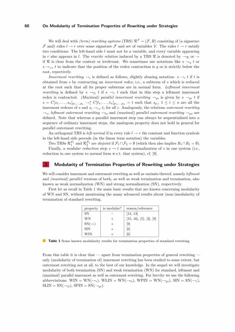
60 On Modularity of Termination Properties of Rewriting under Strategies
We will deal with (term) rewriting systems (TRS) RF = (F , R) consisting of (a signature
F and) rules l → r over some signature F and set of variables V. The rules l → r satisfy
two conditions: The left-hand side l must not be a variable, and every variable appearing
in r also appears in l. The rewrite relation induced by a TRS R is denoted by →R or →
if R is clear from the context or irrelevant. We sometimes use notations like s →q t or
s →>ǫ t to indicate that the position of the redex contraction is q or is strictly below the
root, repectively.
Innermost rewriting →i is defined as follows, slightly abusing notation: s →i t if t is
obtained from s by contracting an innermost redex, i.e., a subterm of s which is reduced
at the root such that all its proper subterms are in normal form. Leftmost innermost
rewriting is defined by s →li t if s →i t such that in this step a leftmost innermost
redex is contracted. (Maximal) parallel innermost rewriting →pi is given by s →pi t if
s = C[s1, . . . , sn]p1,...,pn →∗i C[t1, . . . , tn]p1,...,pn = t such that spi , 1 ≤ i ≤ n are all the
innermost redexes of s and si →i,ǫ ti for all i. Analogously, the relations outermost rewriting
→o, leftmost outermost rewriting →lo and (maximal) parallel outermost rewriting →po are
defined. Note that whereas a parallel innermost step can always be sequentialized into a
sequence of ordinary innermost steps, the analogous property does not hold in general for
parallel outermost rewriting.
An orthogonal TRS is left-normal if in every rule l→ r the constant and function symbols
in the left-hand side precede (in the linear term notation) the variables.
Two TRSs RF1
1 and RF2
2 are disjoint if F1∩F2 = ∅ (which then also implies R1∩R1 = ∅).
Finally, a modular reduction step s t means normalization of s in one system (i.e.,
reduction in one system to normal form w.r.t. that system), cf. [9].
3 Modularity of Termination Properties of Rewriting under Strategies
We will consider innermost and outermost rewriting as well as variants thereof, namely leftmost
and (maximal) parallel versions of both, as well as weak termination and termination, also
known as weak normalization (WN) and strong normalization (SN), respectively.
First let us recall in Table 1 the main basic results that are known concerning modularity
of WN and SN, without mentioning the many advanced results about (non-)modularity of
termination of standard rewriting.
property is modular? reason/reference
SN − [14, 13]
WN + [15, 16], [5], [3], [9]
SN( ) + [9]
SIN + [6]
WIN + [6]
Table 1 Some known modularity results for termination properties of standard rewriting
From this table it is clear that — apart from termination properties of general rewriting —
only (modularity of termination of) innermost rewriting has been studied to some extent, but
outermost rewriting not at all, to the best of our knowledge. In the sequel we will investigate
modularity of both termination (SN) and weak termination (WN) for standard, leftmost and
(maximal) parallel innermost as well as outermost rewriting. For brevity we use the following
abbreviations: WIN = WN(→i), WLIN = WN(→li), WPIN = WN(→pi), SIN = SN(→i),
SLIN = SN(→li), SPIN = SN(→pi).
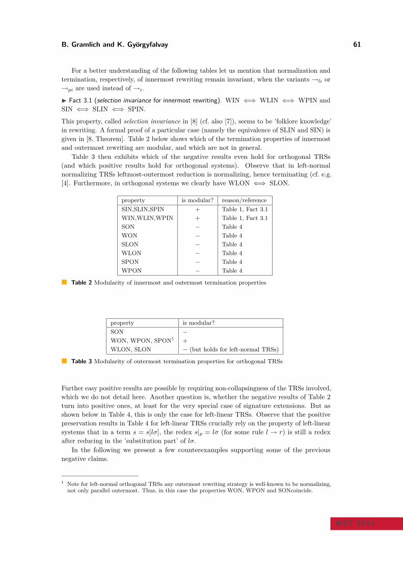
B. Gramlich and K. Györgyfalvay 61
For a better understanding of the following tables let us mention that normalization and
termination, respectively, of innermost rewriting remain invariant, when the variants →li or
→pi are used instead of →i.
Fact 3.1 (selection invariance for innermost rewriting). WIN ⇐⇒ WLIN ⇐⇒ WPIN and
SIN ⇐⇒ SLIN ⇐⇒ SPIN.
This property, called selection invariance in [8] (cf. also [7]), seems to be ’folklore knowledge’
in rewriting. A formal proof of a particular case (namely the equivalence of SLIN and SIN) is
given in [8, Theorem]. Table 2 below shows which of the termination properties of innermost
and outermost rewriting are modular, and which are not in general.
Table 3 then exhibits which of the negative results even hold for orthogonal TRSs
(and which positive results hold for orthogonal systems). Observe that in left-normal
normalizing TRSs leftmost-outermost reduction is normalizing, hence terminating (cf. e.g.
[4]. Furthermore, in orthogonal systems we clearly have WLON ⇐⇒ SLON.
property is modular? reason/reference
SIN,SLIN,SPIN + Table 1, Fact 3.1
WIN,WLIN,WPIN + Table 1, Fact 3.1
SON − Table 4
WON − Table 4
SLON − Table 4
WLON − Table 4
SPON − Table 4
WPON − Table 4
Table 2 Modularity of innermost and outermost termination properties
property is modular?
SON −
WON, WPON, SPON1 +
WLON, SLON − (but holds for left-normal TRSs)
Table 3 Modularity of outermost termination properties for orthogonal TRSs
Further easy positive results are possible by requiring non-collapsingness of the TRSs involved,
which we do not detail here. Another question is, whether the negative results of Table 2
turn into positive ones, at least for the very special case of signature extensions. But as
shown below in Table 4, this is only the case for left-linear TRSs. Observe that the positive
preservation results in Table 4 for left-linear TRSs crucially rely on the property of left-linear
systems that in a term s = s[lσ], the redex s|p = lσ (for some rule l → r) is still a redex
after reducing in the ’substitution part’ of lσ.
In the following we present a few counterexamples supporting some of the previous
negative claims.
1 Note for left-normal orthogonal TRSs any outermost rewriting strategy is well-known to be normalizing,not only parallel outermost. Thus, in this case the properties WON, WPON and SONcoincide.
WST 2012
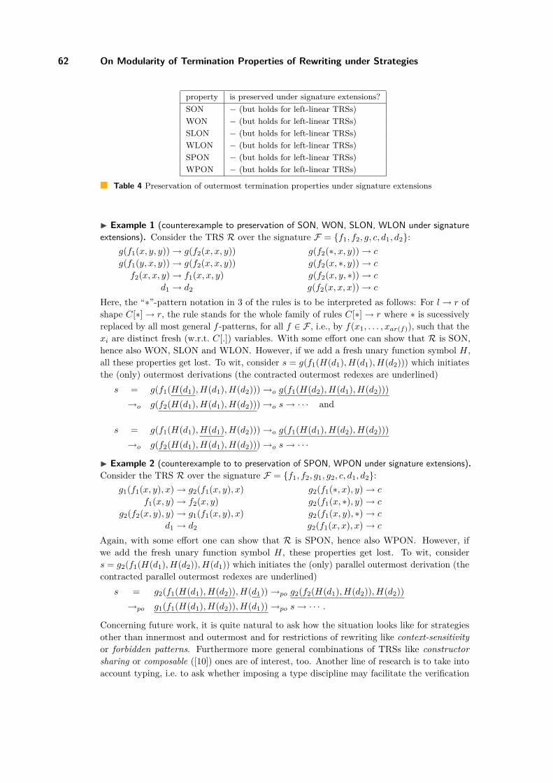
62 On Modularity of Termination Properties of Rewriting under Strategies
property is preserved under signature extensions?
SON − (but holds for left-linear TRSs)
WON − (but holds for left-linear TRSs)
SLON − (but holds for left-linear TRSs)
WLON − (but holds for left-linear TRSs)
SPON − (but holds for left-linear TRSs)
WPON − (but holds for left-linear TRSs)
Table 4 Preservation of outermost termination properties under signature extensions
Example 1 (counterexample to preservation of SON, WON, SLON, WLON under signature
extensions). Consider the TRS R over the signature F = f1, f2, g, c, d1, d2:
g(f1(x, y, y))→ g(f2(x, x, y))
g(f1(y, x, y))→ g(f2(x, x, y))
f2(x, x, y)→ f1(x, x, y)
d1 → d2
g(f2(∗, x, y))→ c
g(f2(x, ∗, y))→ c
g(f2(x, y, ∗))→ c
g(f2(x, x, x))→ c
Here, the “∗”-pattern notation in 3 of the rules is to be interpreted as follows: For l→ r of
shape C[∗]→ r, the rule stands for the whole family of rules C[∗]→ r where ∗ is sucessively
replaced by all most general f -patterns, for all f ∈ F , i.e., by f(x1, . . . , xar(f)), such that the
xi are distinct fresh (w.r.t. C[.]) variables. With some effort one can show that R is SON,
hence also WON, SLON and WLON. However, if we add a fresh unary function symbol H,
all these properties get lost. To wit, consider s = g(f1(H(d1), H(d1), H(d2))) which initiates
the (only) outermost derivations (the contracted outermost redexes are underlined)
s = g(f1(H(d1), H(d1), H(d2)))→o g(f1(H(d2), H(d1), H(d2)))
→o g(f2(H(d1), H(d1), H(d2)))→o s→ · · · and
s = g(f1(H(d1), H(d1), H(d2)))→o g(f1(H(d1), H(d2), H(d2)))
→o g(f2(H(d1), H(d1), H(d2)))→o s→ · · ·
Example 2 (counterexample to to preservation of SPON, WPON under signature extensions).
Consider the TRS R over the signature F = f1, f2, g1, g2, c, d1, d2:
g1(f1(x, y), x)→ g2(f1(x, y), x)
f1(x, y)→ f2(x, y)
g2(f2(x, y), y)→ g1(f1(x, y), x)
d1 → d2
g2(f1(∗, x), y)→ c
g2(f1(x, ∗), y)→ c
g2(f1(x, y), ∗)→ c
g2(f1(x, x), x)→ c
Again, with some effort one can show that R is SPON, hence also WPON. However, if
we add the fresh unary function symbol H, these properties get lost. To wit, consider
s = g2(f1(H(d1), H(d2)), H(d1)) which initiates the (only) parallel outermost derivation (the
contracted parallel outermost redexes are underlined)
s = g2(f1(H(d1), H(d2)), H(d1))→po g2(f2(H(d1), H(d2)), H(d2))
→po g1(f1(H(d1), H(d2)), H(d1))→po s→ · · · .
Concerning future work, it is quite natural to ask how the situation looks like for strategies
other than innermost and outermost and for restrictions of rewriting like context-sensitivity
or forbidden patterns. Furthermore more general combinations of TRSs like constructor
sharing or composable ([10]) ones are of interest, too. Another line of research is to take into
account typing, i.e. to ask whether imposing a type discipline may facilitate the verification
B. Gramlich and K. Györgyfalvay 63
of termination properties of rewriting under strategies, cf. e.g. [17, 1]. On a more technical
level it appears interesting to investigate relationships to other settings and approaches
where non-left-linearity causes major problems, e.g., in (automatically) proving outermost
termination and in dependency pair based termination proofs where signature extensions
play a major role ([12]).
References
1 Takahito Aota and Yoshihito Toyama. Persistency of confluence. Journal of Universal
Computer Science, 3(11):1134–1147, 1997.
2 Franz Baader and Tobias Nipkow. Term rewriting and All That. CUP, 1998.
3 J.A. Bergstra, Jan Willem Klop, and Aart Middeldorp. Termherschrijfsystemen. Deventer,
1989. In Dutch.
4 Marc Bezem, Jan Willem Klop, and Roel de Vrijer, editors. Term Rewriting Systems.
Cambridge Tracts in Theoretical Computer Science 55. CUP, March 2003.
5 Klaus Drosten. Termersetzungssysteme. Informatik-Fachberichte 210. Springer-Verlag,
1989. In German.
6 Bernhard Gramlich. Abstract relations between restricted termination and confluence prop-
erties of rewrite systems. Fundamenta Informaticae, 24:3–23, 1995.
7 M.R.K. Krishna Rao. Relating confluence, innermost-confluence and outermost-confluence
properties of term rewriting systems. Acta Informatica, 33:595–606, 1996.
8 M.R.K. Krishna Rao. Some characteristics of strong innermost normalization. Theoretical
Computer Science, 239(1):141–164, May 2000.
9 Masahito Kurihara and Ikuo Kaji. Modular term rewriting systems and the termination.
Information Processing Letters, 34:1–4, 1990.
10 Enno Ohlebusch. Modular properties of composable term rewriting systems. Journal of
Symbolic Computation, 20(1):1–42, July 1995.
11 Enno Ohlebusch. Advanced Topics in Term Rewriting. Springer-Verlag, 2002.
12 Christian Sternagel and René Thiemann. Signature extensions preserve termination - an al-
ternative proof via dependency pairs. In Anuj Dawar and Helmut Veith, editors, Proc. 19th
Annual Conference of the EACSL (CSL 2010), LNCS 6247, pages 514–528, 2010.
13 Yoshihito Toyama. Counterexamples to termination for the direct sum of term rewriting
systems. Information Processing Letters, 25:141–143, 1987.
14 Yoshihito Toyama. On the Church-Rosser property for the direct sum of term rewriting
systems. Journal of the ACM, 34(1):128–143, 1987.
15 Yoshihito Toyama, Jan Willem Klop, and Henk Pieter Barendregt. Termination for the di-
rect sum of left-linear term rewriting systems. In N. Dershowitz, ed., Proc. 3rd Int. Conf. on
Rewriting Techniques and Applications (RTA’89), LNCS 355, pages 477–491. 1989.
16 Yoshihito Toyama, Jan Willem Klop, and Henk Pieter Barendregt. Termination for direct
sums of left-linear complete term rewriting systems. Journal of the ACM, 42(6):1275–1304,
1995.
17 Hans Zantema. Termination of term rewriting: Interpretation and type elimination. Journal
of Symbolic Computation, 17:23–50, 1994.
WST 2012
Termination Graphs Revisited∗
Georg Moser and Michael Schaper
Institute of Computer Science, University of Innsbruck, Austria
georg.moser,[email protected]
Abstract
We revisit termination graphs from the viewpoint of runtime complexity. Suitably generalising the
construction proposed in the literature, we define an alternative representation of Jinja Bytecode
(JBC) executions as computation graphs. We show that the transformation from JBC programs
to computation graphs is sound, i.e., an infinite execution gives rise to an infinite path in the
computation graph. Moreover, we establish that the transformation is complexity preserving.
1998 ACM Subject Classification F.3.2 - Program analysis
Keywords and phrases Jinja, Runtime Complexity, Rewriting, Computation Graph
1 Introduction
In [9, 4, 3] termination of Jinja Bytecode (JBC for short) programs is studied. To this extent
the execution of a JBC program P is represented in a finite graph, a so-called termination
graph. Based on this graph, integer term rewrite systems R (cf. [5]) are defined, such that
termination of R yields termination of P . That is, the proposed transformation from JBC
to rewrite systems is non-termination preserving.
In this note we revisit termination graphs from the viewpoint of runtime complexity.
Suitably generalising the earlier construction, we propose an alternative representation of
JBC executions in graph form as computation graphs G. The nodes of the computation
graph are abstract states, representing sets of states of the Jinja Virtual Machine (JVM).
The edges represent symbolic evaluations together with refinements and abstraction steps.
We show that the transformation from JBC programs to computation graphs is non-
termination preserving, that is, any infinite evaluation of P gives rise to the existence of
infinite paths in G. Moreover, we establish that the transformation is complexity preserving.
For this we measure the runtime complexity of P as a function that relates the maximal
length of evaluations to the size of the initial state. (Note that this measure overestimates
the size of the input to P only by a constant factor.) Moreover, the computation complexity
maps the maximal length of a path in G to the size of the initial abstract state. We show
that the runtime complexity of P is asymptotically bounded in the computation complexity
of G. Disregarding the viewpoint of complexity, this paper provides a simplification and
clarification of the concepts proposed in [9, 4, 3] and thus may be of independent interest.
In the following we give a brief overview about the Jinja source language, cf. [7] for details.
Values are either Boolean, integers, references, the null reference (denoted as null), or the
dummy value (denoted as unit). We usually refer to (non-null) references as addresses. The
dummy value unit is used for the evaluation of assignments (see [7]) and also used in the
JVM to allocate uninitialised local variables.
A Jinja program consists of a set of class declarations. Each class is identified by a class
name and further consists of the name of its direct superclass, field declarations and method
∗ This work is partially supported by FWF (Austrian Science Fund) project I-608-N18.
© G. Moser and M. Schaper;
licensed under Creative Commons License NC-ND
WST 2012: 12th International Workshop on Termination.
Editor: G. Moser; pp. 64–68

G. Moser and M. Schaper 65
declarations. A field declaration is a pair of field name and field type. A method declaration
consists of the method name, a list of parameter types, the result type and the method body.
The method body consists of a list of parameter identifiers and an expression. The definition
for JBC programs is almost identical to the definition of Jinja programs. The sole exception
is that the JBC method body is represented by a triple (mxs,mxl, ins), where mxs denotes
the maximal size of the operand stack, mxl the number of registers (not including the this
pointer and the parameters) and ins a sequence of JBC instructions. We consider Jinja
programs and JBC programs to be well-formed [7]. Further, we presuppose normal evaluation,
that is, no exceptions are raised and demand that all data structures are non-cyclic.
JBC is executable on the JVM. A state of the JVM is represented by a pair of heap and
frames. The heap represents the global memory of the program and associates addresses
to objects. A frame represents the execution environment of a method and is a quintuple
(stk, loc, cn,mn, pc) such that: stk denotes the operand stack, loc denotes the registers, cn
denotes the class name, mn denotes the method name, and pc is the program counter. Both,
operand stack and registers store values. For each frame the number of registers is fixed and
the maximum size of the operand stack is computed during compilation. Thus the operand
stack can be conceived as an array. See [7] for further details.
2 Abstract States
We extend Jinja by abstract variables Class for each class considered. Further, Bool :=
true, false denotes an abstract Boolean value and any interval I ⊆ [−∞,∞] denotes an
abstract integer value. We write Int instead of I, if the concrete interval is not relevant and
we identify the interval [z, z], where z ∈ Z with the integer z. An abstract value is either a
Jinja value, or an abstract Boolean or integer value. Furthermore, we make use of an infinite
supply of abstract locations ζ0, ζ1, ζ2, . . . In the following denotes the subclass relation.
An abstract state is a triple consisting of the heap, the list of frames, and a set of
annotations. A heap is a mapping from addresses to objects, where an object is either
an abstract variable or pair (cn, ft): cn denotes the class name and ft denotes the field
table, i.e., a mapping from (cn′, fieldid) to abstract values, where cn cn′. Let obj be an
object. We define the projections cl and ft as follows: (i) cl(obj) := cn, if obj = (cn, ft), and
cl(obj) := Class, if obj is an abstract variable of type Class. (ii) ft((cn, ft)) := ft. Registers
and operand stack of a frame, now store abstract values. Furthermore, we define annotations
of addresses in a state s, denoted as iu. Annotations are pairs p 6= q of addresses, where
p, q ∈ heap and p 6= q. The intuition of iu is to express that for p 6= q ∈ iu, we disallow
sharing of these addresses in concrete states. An abstract state which does not contain
abstract variables and where addresses cannot be shared further is a concrete (or Jinja) state.
We define a bijection φ that associates every non-address value in heap with an abstract
location. We define the graph Φ as function of heap:
Φ(heap) := (ζ, val) | ∃ address a: rg(ft(heap(a))) = val, val not an address, ζ fresh .
Finally, we set φ(ζ) := val if (ζ, val) ∈ Φ(heap).
Definition 1. We represent heap as a directed graph H = (VH , SuccH , LH , EH), where
the nodes, the successor relation and the labeling function are defined as follows: (i) VH :=
dom(heap) ∪ dom(φ) (ii) SuccH(u) := [ft∗((C1, id1)), . . . , ft∗((Ck, idk))], if u is an address,
ft(heap(u)) = ft and dom(ft) = (C1, id1), . . . , (Ck, idk), otherwise SuccH(u) := []. Here
ft∗((C, id)) := ft((C, id)), if ft((C, id)) is an address and ft∗((C, id)) := φ−1(ft((C, id)))
otherwise. (iii) LH(u) := cl(heap(u)), if u is an address and LH(u) := φ(u) otherwise. (iv)
WST 2012
66 Termination Graphs Revisited
EH(u → v) := (C, id), if u is an address, ft(heap(u)) = ft and ft((C, id)) = v. Otherwise
we set EH(u→ v) := ǫ.
We call a value val reachable from an address a in heap, if there exists a path from
a to val in the heap graph of heap. For a given state s = (heap, frms, iu) with top-
frame frm = (stk, loc, cn,mn, pc), we are only concerned with the part of the heap that is
reachable from frm. Let heap frm denote the restriction of heap to all nodes reachable
from stk(i) | i ∈ 1, . . . ,m ∪ loc(i) | i ∈ 1, . . . , n. We generalise the bijection φ so that
also non-address values in the registers and on the operand stack are represented. For that
we define the graph Φ as a function of stk, loc, and heap in the natural way. Finally, we set
φ(ζ) := val if (ζ, val) ∈ Φ(stk, loc, heap).
Definition 2. Let s = (heap, frms, iu) be a state and let frm = (stk, loc, cn,mn, pc) be the
top-frame. Let dom(stk) = 1, . . . ,m and let dom(loc) = 1, . . . , n. Recall that stk can be
conceived as array. We use osi (li) to denote index i of the stack (register i). Moreover suppose
H denotes heapfrm. We define the state graph of s as 5-triple S = (VS , SuccS , LS , ES , iu),
where the first four components denote a directed graph with edge labels and iu denotes a set
of annotations. The nodes, the successor relation, and the labeling function of the directed
graph are defined as follows: (i) VS := 1, . . . ,m+n∪VH∪dom(φ) (ii) SuccS(u) := [stk∗(u)],
if u ∈ 1, . . . ,m. Otherwise, if u ∈ m+ 1, . . . , n, then SuccS(u) := [loc∗(u−m)]. Finally,
if u ∈ VH , then SuccS(u) := SuccH(u). Here stk∗(u) and loc∗(u) is defined like ft∗ as
introduced in Definition 1. (iii) LS(u) := osu, if u ∈ 1, . . . ,m and LS(u) := lu−m, if u ∈
m+ 1, . . . , n. Otherwise, LS(u) := cl(heap(u)), if u is an address. Finally, LS(u) := φ(u).
(iv) ES(u→ v) := EH(u→ v), if u, v ∈ H. Otherwise, we set ES(u→ v) := ǫ.
We often confuse a state s and its representation as a state graph and addresses v with its
corresponding object heap(v). We define a binary relation ⊑ on abstract values. Let v, w be
values. Then v ⊑ w if (i) v ∈ null, unit and either v = w or w ∈ null, Class, Bool, Int,
or (ii) v, w ⊆ [−∞,∞] and v ⊆ w, (iii) v, w ∈ true, false, Bool and either v = w or
w = Bool, or (iv) v, w are class names or abstract class variables and v w. Based on the
definition of ⊑ we introduce the following variant of graph morphism, called state morphism.
Definition 3. Let S, T be state graphs. A state morphism from T to S (denotedm : T → S)
is a function m : VT → VS such that (i) for all u ∈ T , LT (u) ⊒ LS(m(u)), (ii) for all u ∈ T ,
m∗(SuccT (u)) = SuccS(m(u)), and (iii) for all uℓ−→ v ∈ T and m(u)
ℓ′
−→ m(v) ∈ S, ℓ = ℓ′.
If no confusion can arise we refer to a state morphism simply as morphism. It is easy to
see that the composition m1 m2 of two morphisms m1, m2 is again a morphism.
Definition 4. Let s = (heap, frms, iu) and t = (heap′, frms′, iu′) be states. Then t is
an instance of s (denoted as t ⊑ s) if the following conditions hold: (i) all corresponding
program counters in the frame lists frms and frms′ coincide, (ii) there exists a morphism
m : s→ t, and (iii) for all p 6= q ∈ iu we have that m(p) 6= m(q) and iu′ ⊆ m∗(iu). If t an
instance of s, then we call s an abstraction of t, denoted as s ⊒ t.
It is an easy consequence of the composability of morphism that the instance relation ⊑
is transitive. Let s = (heap, frms, iu) be a state and let p, q denote distinct addresses in
heap such that p 6= q 6∈ iu. Then we say p and q are unifiable (denoted as p?= q) if there
exists a state t and a morphism m : s→ t, such that m(p) = m(q).
Definition 5. Let s be a state and let S = (VS , SuccS , LS , ES , iu) be its state graph. The
size of s, denoted |s|, is defined as follows:∑l∈LS|l|, where |l| is abs(l) if l ∈ Z, otherwise 1.
(As usual abs(l) denotes the absolut value of the integer l.)

G. Moser and M. Schaper 67
3 Computation Graph
The operational semantics of the JVM yields the single-step execution of each JBC com-
mand [7]. Based on these instructions, and actually mimicking them quite closely, we define
how abstract states are symbolically evaluated. We write instr_of(C,M) to denote the
instruction list of method M in class C of the considered JBC program P . Furthermore,
we set method(C,M) = (D,Ts, T,mbody) to denote that method M with type signature
M : Ts → T is defined in the superclass D of C and its body is mbody = (mxs,mxl, ins).
See [7] for a suitable implementation of the functions instr_of and method.
Let s = (heap, frms, iu) be an abstract state with top-frame frm = (stk, loc, cn,mn, pc).
Suppose instr = instr_of(C,M)(pc), i.e., the current instruction. By case distinction on
instr, one defines the symbolic evaluation of P . In Definition 6 we have worked out the cases
for Putfield and Invoke. The other cases are left to the reader.
Definition 6. Consider a Putfield F C instruction. Let v be a value and r be an address
such that heap(r) = (D, ft). We set ft′ := ft(C,F ) 7→ v to denote the updating of field
F in ft. Suppose there exists no address p ∈ heap such that r?= p. Then we define the
following step:
(heap, (v :: r :: stk, loc, cn,mn, pc) :: frms, iu)
(heapr 7→ (D, ft′), (stk, loc, cn,mn, pc+ 1) :: frms, iu) .
Now, consider an instruction Invoke M n. Suppose r denotes the address of the calling
object and cl(heap(r)) = C and method(C,M) = (D,Ts, T, (mxs,mxl, ins)). We set:
(heap, (pn−1 :: · · · :: p0 :: r :: stk, loc, cn,mn, pc) :: frms, iu)
(heap, frm′ :: (stk, loc, cn,mn, pc) :: frms, iu) ,
where loc′ := [r, p0, . . . , pn−1] @ units and frm′ = ([], loc′, D,M, 0). Here units denotes an
array of unit-values of size mxl.
In addition to symbolic evaluations, we define refinement steps on abstract states s if the
information given in s is not concrete enough to execute a given instruction. Following [4] we
make use of case distinction, class instance, sharing, and unsharing. We will restrict to an
informal explanation of these refinement steps. Case distinction refines abstract Boolean or
integer values if a symbolic instruction is otherwise not possible as the state is underspecified.
The refinement class instance either replaces an abstract class variable by the null-pointer or
refines the information about the class. Finally, the refinement steps sharing, and unsharing
either explicitly share unifiable addresses p, q by identifying them, or the annotation p 6= q is
added to mark that these references must not be shared. We arrive at the definition of a
computation graph.
Definition 7. A computation graph G = (VG, EG) is a directed graph, where VG are
abstract states and s→ t ∈ EG if either (i) t is obtained from s by a symbolic evaluation,
(ii) t is obtained by a refinement step, or (iii) s ⊑ t holds.
Let G be a computation graph. We write G : s G t to indicate that state t is directly
reachable in G from s. If s is reachable from t in G we write G : s∗G t. Let s and t be
concrete states. Then we denote by P : sjvm−−→1 t the one-step transition relation of the JVM.
If there exists a (normal) evaluation of s to t, we write P : sjvm−−→ t. The next lemma states
that any single-step execution on the JVM can be simulated by at least one step in the
computation graph.
WST 2012
68 Termination Graphs Revisited
Lemma 8. Let s be a state and let s′ be a concrete state such that s′ ⊑ s. Then P : s′jvm−−→1 t
′
implies the existence of a state t such that t′ ⊑ t and G : s+G t.
We define the runtime of a JVM for a given normal evaluation P : sjvm−−→ t as the
number of single-step executions. The computation length denotes the maximal length of
a path in the computation graph G such that G : s∗G t. Recall Definition 5, defining
the size of some state s. We define the runtime complexity with respect to P as follows:
rcj(n) := maxm | P : sjvm−−→ t holds such that the runtime is m and |s| 6 n. Similarly we
set: cc(n) := maxm | G : s∗G t holds such that the computation length is m and |s| 6 n.
Theorem 9. Let s′ and t′ be concrete states. Suppose P : s′jvm−−→ t′. Then there exists an
abstraction s of s′ and a computation G : s∗G t such that t′ ⊑ t. Furthermore rcj ∈ O(cc).
4 Conclusion
In this note we propose computation graphs as suitable representation of the execution of a
JVM. We show that this representation is complexity preserving. In future work it needs
to be clarified whether our result on complexity preservation still holds, if the cycles of the
computation graph are considered separately [9]. Furthermore, the notion of (innermost)
runtime complexity for integer rewrite systems need to be clarified (cf. [6, 2] for the standard
definition of runtime complexity of a rewrite system). Finally, methods for runtime complexity
need to be adapted to integer rewrite systems (cf. [1, 8, 6] for examples of existing techniques).
References
1 M. Avanzini and G. Moser. Dependency Pairs and Polynomial Path Orders. In Proc. of
20th RTA, volume 5595 of LNCS, pages 48–62. Springer Verlag, 2009.
2 M. Avanzini and G. Moser. Closing the gap between runtime complexity and polytime
computability. In Proc. of 21th RTA, Leibniz International Proceedings in Informatics.
Schloss Dagstuhl - Leibniz-Zentrum fuer Informatik, Germany, 2010.
3 M. Brockschmidt, C. Otto, and J. Giesl. Modular termination proofs of recursive java
bytecode programs by term rewriting. In Proc. of 22nd RTA, LIPIcs, pages 155–170, 2011.
4 M. Brockschmidt, C. Otto, C. von Essen, and J. Giesl. Termination Graphs for Java
Bytecode. In Verification, Induction, Termination Analysis, volume 6463 of LNCS, pages
17–37, 2010.
5 C. Fuhs, J. Giesl, M. Plücker, P. Schneider-Kamp, and S. Falke. Proving Termination of
Integer Term Rewriting. In Proc. of 20th RTA, volume 5595 of LNCS, pages 32–47, 2009.
6 N. Hirokawa and G. Moser. Automated complexity analysis based on the dependency pair
method. CoRR, abs/1102.3129, 2011. submitted.
7 G. Klein and T-Nipkow. A machine-checked model for a java-like language, virtual machine,
and compiler. ACM Trans. Program. Lang. Syst., 28(4):619–695, 2006.
8 L. Noschinski, F. Emmes, and J. Giesl. A dependency pair framework for innermost com-
plexity analysis of term rewrite systems. In Proc. of 23rd CADE, volume 6803 of LNCS,
pages 422–438, 2011.
9 C. Otto, M. Brockschmidt, C. v. Essen, and J. Giesl. Automated termination analysis of
Java bytecode by term rewriting. In Proc. of 21th RTA, pages 259–276, 2010.
Matrix Interpretations for Polynomial Derivational
Complexity
Friedrich Neurauter∗ and Aart Middeldorp
Institute of Computer Science, University of Innsbruck, Austria
friedrich.neurauter,[email protected]
Abstract
Matrix interpretations can be used to bound the derivational complexity of term rewrite systems.
In general, the obtained bounds are exponential. In this paper we use joint spectral radius theory
in order to completely characterize matrix interpretations that induce polynomial upper bounds
on the derivational complexity of (compatible) rewrite systems.
1998 ACM Subject Classification F.4.2 - Grammars and Other Rewriting Systems, F.4.1 -
Mathematical Logic: Computational logic.
Keywords and phrases Term rewriting, Termination, Derivational Complexity, Matrix Interpre-
tations
1 Introduction
This paper is concerned with automated complexity analysis of term rewrite systems. Given
a terminating rewrite system, the aim is to obtain information about the maximal length
of rewrite sequences in terms of the size of the initial term. This is known as derivational
complexity. Matrix interpretations [3] are a popular method for automatically proving
termination of rewrite systems. They can readily be used to establish upper bounds on
the derivational complexity of compatible rewrite systems. However, in general, matrix
interpretations induce exponential (rather than polynomial) upper bounds. In order to obtain
polynomial upper bounds, the matrices used in a matrix interpretation must satisfy certain
(additional) restrictions, the study of which is the central concern of [8, 9, 11]. So what are
the conditions for polynomial boundedness of a matrix interpretation? In the literature, two
different approaches have emerged. On the one hand, there is the automata-based approach
of [11], where matrices are viewed as weighted (word) automata computing a weight function,
which is required to be polynomially bounded. The result is a complete characterization (i.e.,
necessary and sufficient conditions) of polynomially bounded matrix interpretations over N.
On the other hand, there is the algebraic approach pursued in [9] (originating from [8]) that
can handle matrix interpretations over N, Q, and R but only provides sufficient conditions for
polynomial boundedness. In what follows, we use joint spectral radius theory [5, 4] to extend
the latter to a complete characterization of polynomially bounded matrix interpretations
over N, Q and R.
2 Preliminaries
We assume familiarity with the basics of term rewriting [1, 10]. Let V denote a countably
infinite set of variables and F a fixed-arity signature. The set of terms over F and V is
denoted by T (F ,V). The size |t| of a term t is defined as the number of function symbols and
∗ Friedrich Neurauter is supported by a grant of the University of Innsbruck.
© F. Neurauter and A. Middeldorp;
licensed under Creative Commons License NC-ND
WST 2012: 12th International Workshop on Termination.
Editor: G. Moser; pp. 69–73
70 Matrix Interpretations
variables occurring in it. A term rewrite system (TRS for short) R over T (F ,V) is a finite
set of rewrite rules ℓ→ r such that ℓ /∈ V and Var(ℓ) ⊇ Var(r). The smallest rewrite relation
that contains R is denoted by→R. As usual,→+R
(→∗R) denotes the transitive (and reflexive)
closure of →R and →nR its n-th iterate. For a terminating TRS R, the derivation height of a
term t with respect to R is defined as dh(t,→R) = max n | t→nR u for some term u. The
derivational complexity of R is the function dcR : N\0 → N, k 7→ max dh(t,→R) | |t| 6 k.
An F -algebra A consists of a carrier set A and a collection of interpretations fA : Ak → A
for each k-ary function symbol f ∈ F . By [α]A(·) we denote the usual evaluation function of
A according to an assignment α which maps variables to values in A. An F -algebra together
with a well-founded order > on A is called a (well-founded) monotone algebra if for each
function symbol f ∈ F the interpretation function fA is monotone with respect to > in all
arguments. Any monotone algebra (A, >) (or just A if > is clear from the context) induces
a well-founded order on terms: s >A t if and only if [α]A(s) > [α]A(t) for all assignments α.
A TRS R and a monotone algebra A are compatible if ℓ >A r for all ℓ→ r ∈ R.
Let R be a commutative ring (e.g., Z, Q, R). The ring of all n-dimensional square
matrices over R is denoted by Rn×n. The set of all non-negative n-dimensional square
matrices of Zn×n (Rn×n) is denoted by Nn×n (Rn×n0 ), and we write AT for the transpose of
a matrix (vector) A. With any matrix A ∈ Rn×n0 we associate a directed (weighted) graph
G(A) on n vertices, numbered from 1 to n, such that there is a directed edge (of weight Aij)
in G(A) from i to j if and only if Aij 6= 0. In this situation, A is said to be the adjacency
matrix of the graph G(A). The weight of a path in G(A) is the product of the weights of
its edges. With a (non-empty) finite set of matrices S ⊆ Rn×n0 we associate the directed
(weighted) graph G(S) := G(M), where M denotes the component-wise maximum of the
matrices in S, i.e., Mij = max Aij | A ∈ S for all 1 6 i, j 6 n. Following [5], we define
a directed graph Gk(S) for k > 2 on nk vertices representing ordered tuples of vertices of
G(S), such that there is an edge from vertex (i1, . . . , ik) to (j1, . . . , jk) if and only if there is
a matrix A ∈ S with Aiℓjℓ > 0 for all ℓ = 1, . . . , k.
For matrix interpretations (over R), we fix a dimension n ∈ N \ 0 and use the set Rn0 as
the carrier of an algebraM, together with the order >δ on Rn0 defined as (x1, x2, . . . , xn)T >δ(y1, y2, . . . , yn)
T if x1 >R,δ y1 and xi >R yi for 2 6 i 6 n. Here x >R,δ y if and only if
x >R y + δ. Each k-ary function symbol f is interpreted by a linear function of the following
shape: fM(~v1, . . . , ~vk) = F1~v1 + · · · + Fk~vk + ~f where ~v1, . . . , ~vk are (column) vectors of
variables, F1, . . . , Fk ∈ Rn×n0 and ~f is a vector in Rn0 . To ensure monotonicity, it suffices that
the top left entry (Fi)11 of each matrix Fi is at least one. Then it is easy to see that (M, >δ)
forms a well-founded monotone algebra for any δ > 0. We obtain matrix interpretations
over Q by restricting to the carrier Qn0 . Similarly, matrix interpretations over N operate
on the carrier Nn and use δ = 1. We denote by SM the set of matrices occurring in (the
interpretation functions of)M. We set SM = 0 in the pathological case whenM contains
no matrices. Further, we denote by SkM = A1 · · ·Ak | Ai ∈ SM, 1 6 i 6 k the set of all
products of length k of matrices taken from SM. For k = 0, this yields the singleton set
S0M = I containing only the identity matrix. Finally, S∗M denotes the (matrix) monoid
generated by SM, i.e., S∗M =⋃∞k=0 S
kM. We often drop the subscriptM if it is clear from
the context.
Let t be an arbitrary term and α0 the assignment that maps every variable to 0. In the
sequel, we abbreviate [α0]M(t) by [t]M (or just [t] ifM is clear from the context), and we
write [t]j (1 6 j 6 n) for the j-th component of [t].
F. Neurauter and A. Middeldorp 71
3 Growth of Matrix Interpretations
Following [11], we define the notion of growth of a matrix interpretation as follows.
Definition 3.1. LetM be a matrix interpretation. The growth function ofM is defined
as growthM(k) = max [t]1 | t is a term and |t| 6 k.
According to [9], for a TRS R and a compatible matrix interpretation M, we have
dh(t,→R) 61δ · [t]1, and therefore dcR(k) 6
1δ · growthM(k). As the growth ofM is at most
exponential (in the worst case), the derivational complexity of the TRSs one can handle
in this way can at most be exponential. This was shown in [3] for matrix interpretations
over N, but the result obviously extends to matrix interpretations over Q and R. In order
to establish polynomial derivational complexity, the matrices occurring inM must satisfy
certain additional properties that guarantee polynomial boundedness of growthM(k).
4 Algebraic Methods for Bounding Polynomial Growth
In this section we study an algebraic approach to characterize polynomial growth of matrix
interpretations (over N, Q, and R). We employ the following definition [7, 8, 9].
Definition 4.1. A matrix interpretationM is polynomially bounded (with degree d ∈ N) if
the growth of the entries of all matrix products in S∗M is polynomial (with degree d) in the
length of such products, i.e., max Mij |M ∈ SkM ∈ O(kd) for all 1 6 i, j 6 n, where n is
the dimension ofM.
Obviously, the condition given in Definition 4.1 is sufficient for polynomial boundedness
of growthM(k). Moreover, as shown in [7], it is also necessary in the following sense. If
growthM(k) is polynomially bounded and M is compatible with a TRS R, then there
exists a matrix interpretation N compatible with R such that growthN (k) = growthM(k)
and the entries of all matrix products in S∗N are of polynomial growth (i.e., N conforms to
Definition 4.1). The proof given in [7] leverages the connection between matrix interpretations
and weighted word automata. This is possible since matrix interpretations correspond to a
rather restricted form of tree automata, called path-separated [6]. The idea is to transform a
matrix interpretation into the corresponding automaton, trim this automaton by removing
useless states and then transform the resulting automaton back into a (compatible) matrix
interpretation. Thus, the interpretation N can be obtained from M by simply dropping
some rows and columns (the ones whose indices correspond to the useless states) in the
matrices and vectors occurring in the interpretation functions ofM.
The relationship between polynomially bounded matrix interpretations and the deriva-
tional complexity of compatible TRSs is as follows (cf. [9, 7]).
Lemma 4.2. Let R be a TRS and M a compatible matrix interpretation. If M is
polynomially bounded with degree d, then dcR(k) ∈ O(kd+1).
In the sequel, we employ joint spectral radius theory [5, 4], a branch of mathematics
dedicated to studying the growth rate of products of matrices taken from a set, to obtain a
complete characterization of polynomially bounded matrix interpretations (over N, Q and R).
All matrix norms ‖·‖ are assumed to be submultiplicative, i.e., ‖AB‖ 6 ‖A‖ · ‖B‖.
Definition 4.3. Let S ⊆ Rn×n be a finite set of real square matrices, and let ‖·‖ denote a
matrix norm. The growth function growthS associated with S is defined as growthS(k, ‖·‖) =
max ‖A1 · · ·Ak‖ | Ai ∈ S, 1 6 i 6 k .
WST 2012
72 Matrix Interpretations
Using the (submultiplicative) matrix norm ‖·‖1 given by the sum of the absolute values of
all matrix entries, we observe that a matrix interpretationM is polynomially bounded (with
degree d) if and only if growthSM(k, ‖·‖1) is polynomial in k (with degree d). The asymptotic
behaviour of growthSM(k, ‖·‖1) can be characterized by the joint spectral radius of SM.
Definition 4.4. Let S ⊆ Rn×n be finite, and let ‖·‖ denote a matrix norm. The joint spectral
radius ρ(S) of S is defined as ρ(S) = limk→∞max ‖A1 · · ·Ak‖1/k | Ai ∈ S, 1 6 i 6 k .
It is well-known that this limit always exists and that it does not depend on the chosen
norm, which follows from the equivalence of all norms in Rn. Because of this and due to the
fact that we are only interested in the asymptotic behaviour of growthS(k, ‖·‖), from now on
we simply write growthS(k). The following theorem (due to [2]) provides a characterization
of polynomial boundedness of growthS(k) by the joint spectral radius of S.
Theorem 4.5 ([2, Theorem 1.2]). Let S ⊆ Rn×n be a finite set of matrices. Then
growthS(k) ∈ O(kd) for some d ∈ N if and only if ρ(S) 6 1. In particular, d 6 n− 1.
Hence, polynomial boundedness of growthS(k) is decidable if ρ(S) 6 1 is decidable. But
it is well-known that the latter is undecidable in general, even if S consists of finitely many
non-negative rational matrices (cf. [5, Theorem 2.6]). However, in case S is a finite set of
non-negative integer matrices, then ρ(S) 6 1 is decidable. In particular, there exists a
polynomial-time algorithm that decides it (cf. [5, Theorem 3.1]). This algorithm is based on
the following lemma.
Lemma 4.6 ([5, Lemma 3.3]). Let S ⊆ Rn×n0 be a finite set of non-negative real square
matrices. Then there is a product A ∈ S∗ such that Aii > 1 for some i ∈ 1, . . . , n if and
only if ρ(S) > 1.
According to [5], for S ⊆ Nn×n, the existence of such a product can be characterized in
terms of the graphs G(S) and G2(S) one can associate with S. More precisely, there is a
product A ∈ S∗ with Aii > 1 if and only if
1. there is a cycle in G(S) containing at least one edge of weight w > 1, or
2. there is a cycle in G2(S) containing at least one vertex (i, i) and at least one vertex (p, q)
with p 6= q.
Hence, we have ρ(S) 6 1 if and only if neither of the two conditions holds, which can
be checked in polynomial time according to [5]. Furthermore, as already mentioned in [5,
Chapter 3], this graph-theoretic characterization does not only hold for non-negative integer
matrices, but for any set of matrices such that all matrix entries are either zero or at least
one (because then all paths in G(S) have weight at least one).
Lemma 4.7. Let S ⊆ Rn×n0 be a finite set of matrices where all matrix entries are either
zero or at least one. Then ρ(S) 6 1 is decidable in polynomial time.
So, in the situation of Lemma 4.7, polynomial boundedness of growthS(k) is decidable in
polynomial time. In addition, the exact degree of growth can be computed in polynomial
time (cf. [5, Theorem 3.3, Lemma 3.2 and Proposition 3.3]).
Theorem 4.8. Let S ⊆ Rn×n0 be a finite set of matrices such that ρ(S) 6 1 and all matrix
entries are either zero or at least one, and let d > 0 be the largest integer possessing the
following property: there exist d different pairs of indices (i1, j1), . . . , (id, jd) such that for
every pair (is, js) the indices is, js are different and there is a product A ∈ S∗ for which
Aisis , Aisjs , Ajsjs > 1, and for each 1 6 s 6 d − 1, there exists B ∈ S∗ with Bjsis+1> 1.
Then growthS(k) ∈ Θ(kd) if d > 1 and growthS(k) ∈ O(kd) if d = 0. Moreover, the growth
rate d is computable in polynomial time and d 6 n− 1.
F. Neurauter and A. Middeldorp 73
Next we elaborate on the ramifications of joint spectral radius theory on complexity
analysis of TRSs via polynomially bounded matrix interpretations. To begin with, we note
that a matrix interpretation M is polynomially bounded if and only if ρ(SM) 6 1. This
follows directly from Theorem 4.5. Due to the relationship between polynomially bounded
matrix interpretations and the derivational complexity of compatible TRSs expressed in
Lemma 4.2, we immediately obtain the following result, which holds for matrix interpretations
over N, Q, and R.
Theorem 4.9. Let R be a TRS andM a compatible matrix interpretation of dimension n.
If ρ(SM) 6 1, then dcR(k) ∈ O(kn).
As this theorem assumes the worst-case growth rate for growthSM(k), the inferred degree
of the polynomial bound may generally be too high (and unnecessarily so). Yet with the
help of Theorem 4.8, from which we obtain the exact growth rate, Theorem 4.9 can be
strengthened (in this respect), at the expense of having to restrict the set of permissible
matrices.
Theorem 4.10. Let R be a TRS andM a compatible matrix interpretation of dimension n
where all matrix entries are either zero or at least one. If ρ(SM) 6 1, then dcR(k) ∈ O(kd+1),
where d refers to the growth rate obtained from Theorem 4.8.
References
1 F. Baader and T. Nipkow. Term Rewriting and All That. Cambridge University Press,
1998.
2 J.P. Bell. A gap result for the norms of semigroups of matrices. LAA, 402:101–110, 2005.
3 J. Endrullis, J. Waldmann, and H. Zantema. Matrix interpretations for proving termination
of term rewriting. JAR, 40(2–3):195–220, 2008.
4 R. M. Jungers, V. Protasov, and V. D. Blondel. Efficient algorithms for deciding the type
of growth of products of integer matrices. LAA, 428(10):2296–2311, 2008.
5 R.M. Jungers. The Joint Spectral Radius: Theory and Applications. Springer Verlag, 2009.
6 A. Koprowski and J. Waldmann. Max/plus tree automata for termination of term rewriting.
AC, 19(2):357–392, 2009.
7 A. Middeldorp, G. Moser, F. Neurauter, J. Waldmann, and H. Zankl. Joint spectral radius
theory for automated complexity analysis of rewrite systems. In CAI 2011, volume 6742 of
LNCS, pages 1–20, 2011.
8 G. Moser, A. Schnabl, and J. Waldmann. Complexity analysis of term rewriting based
on matrix and context dependent interpretations. In FSTTCS 2008, volume 2 of LIPIcs,
pages 304–315, 2008.
9 F. Neurauter, H. Zankl, and A. Middeldorp. Revisiting matrix interpretations for polyno-
mial derivational complexity of term rewriting. In LPAR-17, volume 6397 of LNCS, pages
550–564, 2010.
10 Terese. Term Rewriting Systems, volume 55 of Cambridge Tracts in Theoretical Computer
Science. Cambridge University Press, 2003.
11 J. Waldmann. Polynomially bounded matrix interpretations. In RTA 2010, volume 6 of
LIPIcs, pages 357–372, 2010.
WST 2012
Encoding Induction in Correctness Proofs of
Program Transformations as a Termination
Problem∗
Conrad Rau, David Sabel, and Manfred Schmidt-Schauß
Dept. Informatik und Mathematik, Inst. Informatik, Goethe-University
D-60054 Frankfurt, Germany
rau,sabel,[email protected]
Abstract
The diagram-based method to prove correctness of program transformations consists of comput-
ing complete set of (forking and commuting) diagrams, acting on sequences of standard reductions
and program transformations. In many cases, the only missing step for proving correctness of a
program transformation is to show the termination of the rearrangement of the sequences. There-
fore we encode complete sets of diagrams as term rewriting systems and use an automated tool
to show termination, which provides a further step in the automation of the inductive step in
correctness proofs.
1998 ACM Subject Classification F.3.1 - Specifying and Verifying and Reasoning about Pro-
grams, F.3.2 - Semantics of Programming Languages
Keywords and phrases Termination, Program Transformations, Correctness
1 Introduction
The motivation for this work is derived from proving correctness of program transformations
in program calculi, in particular in extended lambda calculi that model core-languages of
variants of Haskell.
In our setting a program calculus is a tuple (E , C,sr−→,A) where E is the set of expressions,
C is the set of contexts, i.e. usually C consists of all expressions of E where one subexpression
is replaced by the context hole,sr−→ ⊆ E×E is a small-step reduction relation (called standard
reduction) which defines the operational semantics of the program calculus and A ⊆ E is a
set of answers, which are usuallysr−→-irreducible. The evaluation of a program expression
e ∈ E is a sequence of standard reduction steps to an answer a ∈ A, i.e. esr,∗−−→ a, where
sr,∗−−→ denotes the reflexive-transitive closure of
sr−→. If such an evaluation exists, then we
write e⇓ and say e converges, otherwise we write e⇑ and say e diverges. The semantics
is the contextual equivalence of expressions: e ∼c e′ : ⇐⇒ e ≤c e
′ ∧ e′ ≤c e, where
e ≤c e′ :⇐⇒ ∀C ∈ C : C[e]⇓ =⇒ C[e′]⇓.
A program transformationT−→ ⊆ (E × E) is a binary relation on expressions. It is called
correct if for all e, e′ with eT−→ e′ the equivalence e ∼c e
′ holds. Usually a context-closure T ′ of
the program transformation T is considered (w.r.t. all contexts, or a restricted class of contexts,
if a context lemma is available), such that proving eT ′
−→ e′ implies e⇓ ⇐⇒ e′⇓ suffices to
conclude that T is a correct program transformation. In the following we do not distinguish
between T and its context-closure T ′, and assume that a program transformation is always
closed by an appropriate class of contexts such that the correctness proof is reduced to show
∗ This work was supported by the DFG under grant SCHM 986/9-1.
© C. Rau, D. Sabel, and M. Schmidt-Schauß;
licensed under Creative Commons License NC-ND
WST 2012: 12th International Workshop on Termination.
Editor: G. Moser; pp. 74–78
C. Rau, D. Sabel, and M. Schmidt-Schauß 75
equivalence of convergence for all eT−→ e′. Moreover, with
T←− denoting the inverse of
T−→
the correctness ofT−→ holds, if
T−→ as well as
T←− are convergence preserving (where
T−→ is
convergence preserving if eT−→ e′ =⇒ (e⇓ =⇒ e′⇓)).
In the application below, we will use different program transformations T1, . . . , Tk in
which case we set T =⋃ki=1 Ti. In general, there are also different kinds of standard
reductions, which are used in the concrete proofs, hence we extend the standard reduction tosr−→ ⊆ E ×E ×L where L is a set of labels. Sometimes we indicate the label l by writing
sr,l−−→.
We say the program transformationT−→ is answer-preserving, if a ∈ A and a
T−→ e implies
e ∈ A; and weakly answer-preserving, if a ∈ A and aT−→ e implies e⇓.
The diagram-based proof method operates on abstract reduction sequences (ARS), which
are strings consisting only of the standard reductions with their labels, and the program
transformations, but the expressions are ignored with the exception of an abstract symbol
A for an answer. A forking diagram is a rewriting rule L R on ARSs. The semantics of
a diagram L R is that the reduction sequence L can be transformed (or rewritten) into
the reduction sequence R. We also allow diagrams that speak about transitive closures of
reductions. We are only interested in ARSs that are a mix ofsr←− and
T−→-reductions, perhaps
labeled, together with an answer token A to the left. The idea of the diagrams is that they
transform reduction sequences into evaluations. In general, this rewriting is non-deterministic,
which is the price for abstracting away the term structure. Completeness of a set DF (T−→) of
forking diagrams for transformationT−→ means that every ARS A
sr,+←−−−
T−→ is modifiable by
a diagram. ForT←− we call the diagrams in DF (
T←−) commuting diagrams.
Usually, forking diagrams are of the formsr,ln←−−− . . .
sr,l1←−−−
Tk−→
T1−→ . . .
Tm−−→
sr,ln′
←−−− . . .sr,l1←−−−
where labels li may also be omitted and where also the meta-symbols + and ∗ may occur for
the transitive/transitive-reflexive closure of a standard reduction or transformation.
We also need another form of diagrams, the answer diagrams, DA(T−→), which are called
complete (for transformationT−→), if every ARS A
T,+−−→ is modifiable by a diagram in DA. In
the case of answer-preservation, these extra diagrams are simply AT−→ A, and for a weakly
answer-preserving transformation, the diagrams are of the form AT−→ A
sr,ln←−−− . . .
sr,l1←−−−,
where usually only a subset of the labels occur as li which may ease the termination proof.
In applications to calculi, the computation of the diagram sets for a given program
transformation is done by analyzing the syntax of expressions and the syntax of rules and
by covering all possibilities, where usually labels are heavily used atsr←−, depending on the
kind of reduction rules, and often, several program transformations occur in the diagram set.
This computation may be done by hand, but there is also a proposal for automating this in
an expressive core calculus of Haskell, see [3, 4].
The diagram based method to show correctness of a program transformationT−→ is
performed by the steps:
1. Show (weak) answer-preservation ofT−→ and compute the DA-diagrams.
2. Compute complete sets of forking-diagrams forT−→.
3. Show that every reduction sequence asr,∗←−− e
T−→ e′ where a ∈ A can be transformed
using the diagrams from steps 1 and 2 into a′sr,∗←−− e′, where a′ ∈ A. This is usually done
by an induction on the application of diagrams.
4. Do the same by performing steps (1), (2), (3) for the inverse relationT←−.
Since answer-preservation implies weak answer-preservation, we show the next theorem
only for the weak case.
WST 2012
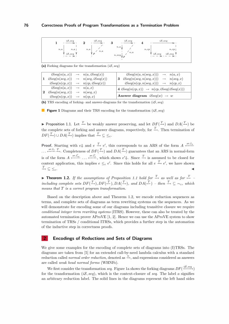
76 Correctness Proofs of Program Transformations as a Termination Problem
1 ·iS,seq
//
n,a
·
n,a
·iS,seq
//___ ·
2 ·iS,seq
//
n,a
·
n,a
·
3 ·iS,seq
//
n,a
·
n,a
·
n,seq·
4 ·iS,seq
//
n,cp
·
n,cp
·iS,seq
//___ ·iS,seq
//___ ·
(a) Forking diagrams for the transformation (iS, seq)
1
iSseq(n(a, x)) → n(a, iSseq(x))
iSseq(n(seq, x)) → n(seq, iSseq(x))
iSseq(n(cp, x)) → n(cp, iSseq(x))
3
iSseq(n(a, n(seq, x))) → n(a, x)
iSseq(n(seq, n(seq, x))) → n(seq, x)
iSseq(n(cp, n(seq, x))) → n(cp, x)
2
iSseq(n(a, x)) → n(a, x)
iSseq(n(seq, x)) → n(seq, x)
iSseq(n(cp, x)) → n(cp, x)
4 iSseq(n(cp, x)) → n(cp, iSseq(iSseq(x)))
Answer diagram iSseq(w) → w
(b) TRS encoding of forking- and answer-diagrams for the transformation (iS, seq)
Figure 1 Diagrams and their TRS encoding for the transformation (iS, seq)
Proposition 1.1. LetT−→ be weakly answer preserving, and let DF (
T−→) and DA(
T−→) be
the complete sets of forking and answer diagrams, respectively, forT−→. Then termination of
DF (T−→) ∪DA(
T−→) implies that
T−→ ⊆ ≤c.
Proof. Starting with e⇓ and eT−→ e′, this corresponds to an ARS of the form A
sr,ln←−−−
. . .sr,l1←−−−
T−→. Completeness of DF (
T−→) and DA(
T−→) guarantees that an ARS in normal-form
is of the form Asr,l′
m
←−−− . . .sr,l′1←−−−, which shows e′⇓. Since
T−→ is assumed to be closed for
context application, this implies e ≤c e′. Since this holds for all e
T−→ e′, we have shown
T−→ ⊆ ≤c.
Theorem 1.2. If the assumptions of Proposition 1.1 hold forT−→ as well as for
T←− –
including complete sets DF (T−→), DF (
T←−), DA(
T−→), and DA(
T←−) – then
T−→ ⊆ ∼c, which
means that T is a correct program transformation.
Based on the description above and Theorem 1.2, we encode reduction sequences as
terms, and complete sets of diagrams as term rewriting systems on the sequences. As we
will demonstrate for encoding some of our diagrams including transitive closure we require
conditional integer term rewriting systems (ITRS). However, these can also be treated by the
automated termination prover AProVE [1, 2]. Hence we can use the AProVE system to show
termination of TRSs / conditional ITRSs, which provides a further step in the automation
of the inductive step in correctness proofs.
2 Encodings of Reductions and Sets of Diagrams
We give some examples for the encoding of complete sets of diagrams into (I)TRSs. The
diagrams are taken from [5] for an extended call-by-need lambda calculus with a standard
reduction called normal order reduction, denoted asn−→, and expressions considered as answers
are called weak head normal forms (WHNFs).
We first consider the transformation seq. Figure 1a shows the forking diagrams DF(iS,seq−−−−→)
for the transformation (iS, seq), which is the context-closure of seq. The label a signifies
an arbitrary reduction label. The solid lines in the diagrams represent the left hand sides
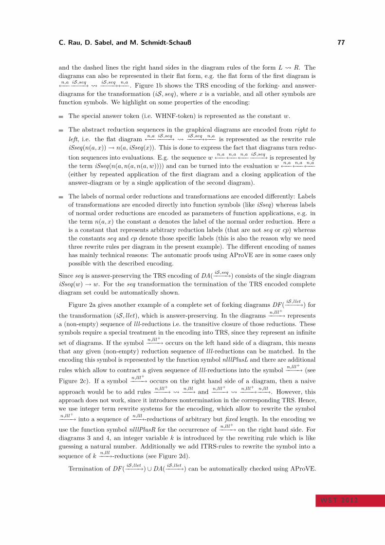
C. Rau, D. Sabel, and M. Schmidt-Schauß 77
and the dashed lines the right hand sides in the diagram rules of the form L R. The
diagrams can also be represented in their flat form, e.g. the flat form of the first diagram isn,a←−−
iS,seq−−−−→
iS,seq−−−−→
n,a←−−. Figure 1b shows the TRS encoding of the forking- and answer-
diagrams for the transformation (iS, seq), where x is a variable, and all other symbols are
function symbols. We highlight on some properties of the encoding:
The special answer token (i.e. WHNF-token) is represented as the constant w.
The abstract reduction sequences in the graphical diagrams are encoded from right to
left, i.e. the flat diagramn,a←−−
iS,seq−−−−→
iS,seq−−−−→
n,a←−− is represented as the rewrite rule
iSseq(n(a, x))→ n(a, iSseq(x)). This is done to express the fact that diagrams turn reduc-
tion sequences into evaluations. E.g. the sequence wn,a←−−
n,a←−−
n,a←−−
iS,seq−−−−→ is represented by
the term iSseq(n(a, n(a, n(a,w)))) and can be turned into the evaluation wn,a←−−
n,a←−−
n,a←−−
(either by repeated application of the first diagram and a closing application of the
answer-diagram or by a single application of the second diagram).
The labels of normal order reductions and transformations are encoded differently: Labels
of transformations are encoded directly into function symbols (like iSseq) whereas labels
of normal order reductions are encoded as parameters of function applications, e.g. in
the term n(a, x) the constant a denotes the label of the normal order reduction. Here a
is a constant that represents arbitrary reduction labels (that are not seq or cp) whereas
the constants seq and cp denote those specific labels (this is also the reason why we need
three rewrite rules per diagram in the present example). The different encoding of names
has mainly technical reasons: The automatic proofs using AProVE are in some cases only
possible with the described encoding.
Since seq is answer-preserving the TRS encoding of DA(iS,seq−−−−→) consists of the single diagram
iSseq(w) → w. For the seq transformation the termination of the TRS encoded complete
diagram set could be automatically shown.
Figure 2a gives another example of a complete set of forking diagrams DF(iS,llet−−−−→) for
the transformation (iS, llet), which is answer-preserving. In the diagramsn,lll+
−−−−→ represents
a (non-empty) sequence of l ll-reductions i.e. the transitive closure of those reductions. These
symbols require a special treatment in the encoding into TRS, since they represent an infinite
set of diagrams. If the symboln,lll+
−−−−→ occurs on the left hand side of a diagram, this means
that any given (non-empty) reduction sequence of l ll-reductions can be matched. In the
encoding this symbol is represented by the function symbol nlllPlusL and there are additional
rules which allow to contract a given sequence of l ll-reductions into the symboln,lll+
−−−−→ (see
Figure 2c). If a symboln,lll+
−−−−→ occurs on the right hand side of a diagram, then a naive
approach would be to add rulesn,lll+
−−−−→ n,lll−−−→ and
n,lll+
−−−−→ n,lll+
−−−−→n,lll−−−→. However, this
approach does not work, since it introduces nontermination in the corresponding TRS. Hence,
we use integer term rewrite systems for the encoding, which allow to rewrite the symboln,lll+
−−−−→ into a sequence ofn,lll−−−→-reductions of arbitrary but fixed length. In the encoding we
use the function symbol nlllPlusR for the occurrence ofn,lll+
−−−−→ on the right hand side. For
diagrams 3 and 4, an integer variable k is introduced by the rewriting rule which is like
guessing a natural number. Additionally we add ITRS-rules to rewrite the symbol into a
sequence of kn,lll−−−→-reductions (see Figure 2d).
Termination of DF(iS,llet−−−−→) ∪DA(
iS,llet−−−−→) can be automatically checked using AProVE.
WST 2012
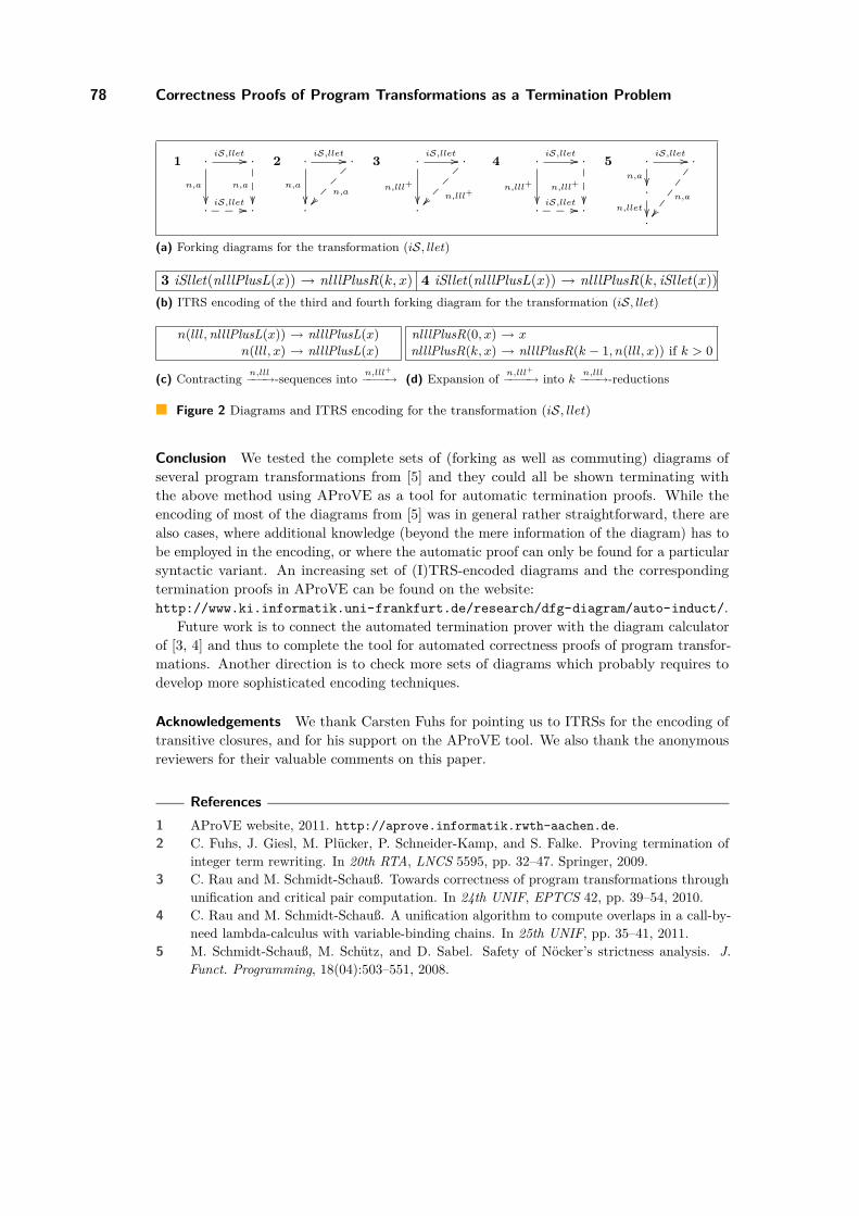
78 Correctness Proofs of Program Transformations as a Termination Problem
1 ·iS,llet
//
n,a
·
n,a
·iS,llet
//___ ·
2 ·iS,llet
//
n,a
·
n,a
·
3 ·iS,llet
//
n,lll+
·
n,lll+
·
4 ·iS,llet
//
n,lll+
·
n,lll+
·iS,llet
//___ ·
5 ·iS,llet
//
n,a
·
n,a
·
n,llet·
(a) Forking diagrams for the transformation (iS, llet)
3 iSllet(nlllPlusL(x)) → nlllPlusR(k, x) 4 iSllet(nlllPlusL(x)) → nlllPlusR(k, iSllet(x))
(b) ITRS encoding of the third and fourth forking diagram for the transformation (iS, llet)
n(lll,nlllPlusL(x)) → nlllPlusL(x)
n(lll, x) → nlllPlusL(x)
(c) Contractingn,lll−−−→-sequences into
n,lll+
−−−−→
nlllPlusR(0, x) → x
nlllPlusR(k, x) → nlllPlusR(k − 1, n(lll, x)) if k > 0
(d) Expansion ofn,lll+
−−−−→ into kn,lll−−−→-reductions
Figure 2 Diagrams and ITRS encoding for the transformation (iS, llet)
Conclusion We tested the complete sets of (forking as well as commuting) diagrams of
several program transformations from [5] and they could all be shown terminating with
the above method using AProVE as a tool for automatic termination proofs. While the
encoding of most of the diagrams from [5] was in general rather straightforward, there are
also cases, where additional knowledge (beyond the mere information of the diagram) has to
be employed in the encoding, or where the automatic proof can only be found for a particular
syntactic variant. An increasing set of (I)TRS-encoded diagrams and the corresponding
termination proofs in AProVE can be found on the website:
http://www.ki.informatik.uni-frankfurt.de/research/dfg-diagram/auto-induct/.
Future work is to connect the automated termination prover with the diagram calculator
of [3, 4] and thus to complete the tool for automated correctness proofs of program transfor-
mations. Another direction is to check more sets of diagrams which probably requires to
develop more sophisticated encoding techniques.
Acknowledgements We thank Carsten Fuhs for pointing us to ITRSs for the encoding of
transitive closures, and for his support on the AProVE tool. We also thank the anonymous
reviewers for their valuable comments on this paper.
References
1 AProVE website, 2011. http://aprove.informatik.rwth-aachen.de.
2 C. Fuhs, J. Giesl, M. Plücker, P. Schneider-Kamp, and S. Falke. Proving termination of
integer term rewriting. In 20th RTA, LNCS 5595, pp. 32–47. Springer, 2009.
3 C. Rau and M. Schmidt-Schauß. Towards correctness of program transformations through
unification and critical pair computation. In 24th UNIF, EPTCS 42, pp. 39–54, 2010.
4 C. Rau and M. Schmidt-Schauß. A unification algorithm to compute overlaps in a call-by-
need lambda-calculus with variable-binding chains. In 25th UNIF, pp. 35–41, 2011.
5 M. Schmidt-Schauß, M. Schütz, and D. Sabel. Safety of Nöcker’s strictness analysis. J.
Funct. Programming, 18(04):503–551, 2008.
A Relative Dependency Pair Framework∗
Christian Sternagel1 and René Thiemann2
1 School of Information Science,
Japan Advanced Institute of Science and Technology, Japan
2 Institute of Computer Science, University of Innsbruck, Austria
1 Introduction
Relative rewriting and the dependency pair framework (DP framework) are two strongly
related termination methods. In both formalisms we consider whether the combination of
two TRSs allows an infinite derivation:
Relative termination of R/S can be defined as strong normalization of →R · →∗S
.
Finiteness of a DP problem (P,R) can be defined as strong normalization ofǫ→P · →
∗R
whereǫ→ allows steps only at the top. Moreover, minimality can be incorporated by
requiring that all terms are terminating w.r.t. R.
The above definitions have two orthogonal distinctions of rules. In both formalisms there
are strict and weak rules: P and R are the strict rules of (P,R) and R/S, respectively,
while R and S are the respective weak rules. In the DP framework, there is the additional
distinction between rules that may only be applied at the top (P) and those that can be
applied at arbitrary positions (R).
Note that the restriction to top rewriting is an important advantage for proving termination
in the DP framework. It allows to use non-monotone orders for orienting the strict rules.
Furthermore, if minimality is considered, we can use termination techniques (e.g., usable
rules or the subterm criterion) that are not available for relative rewriting.
However, also relative rewriting has some advantages which are currently not available in
the DP framework: Geser showed that it is always possible to split a relative termination
problem into two parts [4]. Relative termination of (Rs ∪Rw)/(Ss ∪ Sw) can be shown by
relative termination of both (Rs ∪ Ss)/(Rw ∪ Sw) and Rw/Sw. Hence, it is possible to show
(in a first relative termination proof) that the strict rules Rs∪Ss cannot occur infinitely often
and afterwards continue (in a second relative termination proof) with the problem Rw/Sw. A
major advantage of this approach is that in the first proof we can apply arbitrary techniques
which may increase the size of the TRSs drastically (e.g., semantic labeling [11]), or which
may even be incomplete (e.g., string reversal in combination with innermost rewriting, where
by reversing the rules we have to forget about the strategy). As long as relative termination
of (Rs ∪ Ss)/(Rw ∪ Sw) could be proven, we can afterwards continue independently with the
problem Rw/Sw.
Such a split is currently not possible in the DP framework since there are no top weak
rules and also no strict rules which can be applied everywhere.
In this paper we generalize the DP framework to a relative DP framework, where such a
split is possible. To this end, we consider DP problems of the form (P,Pw,R,Rw), where we
have strict and weak, top and non-top rules. (This kind of DP problems were first suggested
by Jörg Endrullis at the Workshop on the Certification of Termination Proofs in 2007 and
∗ This research is supported by the Austrian Science Fund (FWF): P22767, J3202.
© C. Sternagel and R. Thiemann;
licensed under Creative Commons License NC-ND
WST 2012: 12th International Workshop on Termination.
Editor: G. Moser; pp. 79–83
80 A Relative Dependency Pair Framework
are already used in his termination tool Jambox [3]. Unfortunately the suggestion did not get
much attention back then and we are not aware of any publications on this topic.) In this way,
problems that occur in combination with semantic labeling and dependency pairs—which
can otherwise be solved by using a dedicated semantics for DP problems [9]—can easily be
avoided. Furthermore, the new framework is more general than [9] since it also solves some
problems that occur when using other termination techniques like uncurrying [6, 8].
2 A Relative Dependency Pair Framework
We assume familiarity with term rewriting [2] and the DP framework [5].
Definition 1. A relative dependency pair problem (P,Pw,R,Rw) is a quadruple of TRSs
with pairs P ∪ Pw (where pairs from P are called strict and those of Pw weak) and rules
R∪Rw (where rules of R are called strict and those of Rw weak).
For relative DPPs the notion of chains and finiteness is adapted in the following way.
Definition 2. An infinite sequence of pairs s1 → t1, s2 → t2, . . . forms a (P,Pw,R,Rw)-
chain if there exists a corresponding sequence of substitutions σ1, σ2, . . . such that
si → ti ∈ P ∪ Pw for all i (1)
tiσi →∗
R∪Rw
si+1σi+1 for all i (2)
si → ti ∈ P or tiσi →∗
R∪Rw
· →R · →∗
R∪Rw
si+1σi+1 for infinitely many i (3)
For minimal chains, we additionally require
SNR∪Rw(tiσi) for all i (4)
A relative DPP (P,Pw,R,Rw) is finite, iff there is no minimal infinite (P,Pw,R,Rw)-chain.
Hence, a (minimal) (P,Pw,R,Rw)-chain is like a (minimal) (P ∪Pw,R∪Rw)-chain—as
defined in [1]—with the additional demand that there are infinitely many strict steps using
P or R. It is easy to see that (P,R)-chains can be expressed in the new framework.
Lemma 3. The DP problem (P,R) is finite iff there exists a minimal (P,R)-chain iff
there exists a minimal (P, ∅, ∅,R)-chain iff the relative DPP (P, ∅, ∅,R) is finite.
Note that in contrast to DPPs (P,R), for relative DPPs, P = ∅ does not imply finiteness
of (P,Pw,R,Rw).
Example 4. The relative DPP (∅, F(a)→ F(b), b→ a, ∅) is not finite.
However, a sufficient criterion for finiteness is that there are either no pairs, or that there
are neither strict pairs nor strict rules.
Lemma 5 (Trivially finite relative DPPs). If P ∪Pw = ∅ or P ∪R = ∅ then (P,Pw,R,Rw)
is finite.
3 Processors in the Relative Dependency Pair Framework
Processors and soundness of processors in the relative DP framework are defined as in the DP
framework, but operate on relative DPPs instead of DPPs (a processor is sound if finiteness
of all resulting relative DPPs implies finiteness of the given relative DPP).
C. Sternagel and R. Thiemann 81
Note that most processors can easily be adapted to the new framework where most often
it suffices to treat the relative DPP (P,Pw,R,Rw) as the DPP (P ∪ Pw,R∪Rw).
However, when starting with the initial relative DPP (DP(R), ∅, ∅,R) it is questionable
whether we ever reach relative DPPs containing weak pairs or strict rules. If this is not the
case, then our generalization would be useless. Therefore, in the following we give evidence
that the additional flexibility is beneficial.
Easy examples are semantic labeling and uncurrying. Both techniques are transformational
techniques where each original step is transformed into one main transformed step together
with some auxiliary steps. For the auxiliary steps one uses auxiliary pairs and rules (the
decreasing rules and the uncurrying rules, respectively). If there are auxiliary pairs Paux ,
then in the DP framework, Paux can only be added as strict pairs, whereas in the relative
DP framework, we can add Paux to the weak pairs, and hence we do not have to delete all
pairs of Paux anymore for proving finiteness.
As another example, we consider top-uncurrying of [8, Def. 19], where some rules R are
turned into pairs. Again, in the DP framework this would turn the weak rules R into strict
pairs, which in fact would demand that we prove termination of R twice: Once via the
original DPs for R, and a second time after the weak rules of R have been converted into
strict pairs. For example, in [8, Ex. 21] termination of the minus-rules is proven twice. This
is no longer required in the relative DP framework where one can just turn the weak rules R
into weak pairs R.
Finally, in the relative DP framework we can apply the split technique known from
relative rewriting.
Definition 6 (Split processor). The relative DPP (P1s∪ P1
w,P2
s∪ P2
w,R1
s∪R1
w,R2
s∪R2
w)
is finite if both (P1s∪ P2
s,P1
w∪ P2
w,R1
s∪R2
s,R1
w∪R2
w) and (P1
w,P2
w,R2
w,R2
w) are finite.
A more instructive way of putting the above definition for termination tool authors that
are used to standard DP problems is as follows. Start from the relative DPP (P, ∅, ∅,R).
Identify pairs P ′ and rules R′ that should be deleted. Then use the split processor to obtain
the two relative DPPs (P ′,P \ P ′,R′,R \R′) and (P \ P ′, ∅, ∅,R \R′).
Clearly, the split processor can be used to obtain relative DPPs with strict rules and
weak pairs, but the question is how to apply it. We give two possibilities.
Semantic labeling is often used in a way, that after labeling one tries to remove all labeled
variants of some rules Rs and pairs Ps, and afterwards removes the labels again to continue
on a smaller unlabeled problem.
Example 7. Consider a DP problem p1 = (1, 2, 3). After applying semantic labeling,
all pairs and rules occur in labeled variants 1.x, 2.x, and 3.x, so the resulting DP problem
might look like (1.a, 1.b, 2.a, 2.b, 3.a, 3.b, 3.c). Applying standard techniques to remove
pairs and rules one might get stuck at p2 = (2.a, 2.b, 3.a, 3.c). Although p1 contains less
rules than p2, p2 is somehow simpler since all rules 1.x have been removed. And indeed, after
applying unlabeling on p2 the resulting DP problem p3 = (2, 3) is smaller than p1.
Since the removal of labels is problematic for soundness, a special semantics was developed
in [9]. This is no longer required in the relative DP framework. After Rs and Ps have
been identified, one just applies the split processor to transform (P, ∅, ∅,R) into (Ps,P \
Ps,Rs,R \Rs) and (P \ Ps, ∅, ∅,R \Rs). The proof that all labeled variants of rules in Rs
and pairs in Ps can be dropped, proves finiteness of the first problem, and one can continue
on the latter problem without having to apply unlabeling.
WST 2012
82 A Relative Dependency Pair Framework
Example 8. Using split, we can restructure the proof of Example 7 without using unlabeling:
We know that in the end, we only get rid of pair 1. Hence, we apply split on p1 to obtain
p3 and p4 = (1, 2, ∅, 3). Thus, we get the same remaining problem p3 if we can prove
finiteness of p4. But this can be done by replaying the proof steps in Example 7. Applying
the same labeling as before, we obtain p5 = (1.a, 1.b, 2.a, 2.b, ∅, 3.a, 3.b, 3.c). Removing
pairs and rules as before, we simplify p5 to p6 = (∅, 2.a, 2.b, ∅, 3.a, 3.c) and this relative
DP problem is trivially finite by Lemma 5.
Note that using [9] it was only possible to revert the labeling, but not to revert other
techniques like the closure under flat contexts which is used in combination with root-labeling
[7]. However, using the split processor this is also easily possible, since one just has to apply
the split processor before applying the closure under flat contexts.
A further advantage of the relative DP framework in comparison to [9] can be seen in the
combination of semantic labeling with the dependency graph processor.
Example 9. Consider a DP problem p1 = (1, 2, 3, 4) which is transformed into
(1.a, 1.b, 2.a, 2.b, 3.a, 3.b, 4.a, 4.b) using semantic labeling. Applying the dependency
graph and reduction pairs yields two remaining DP problems p2 = (2.a, 4.a) and
p3 = (2.b, 3.a, 4.b). Using unlabeling we have to prove finiteness of the two remaining
problems p4 = (2, 4) and p5 = (2, 3, 4). Note that finiteness of p5 does not imply
finiteness of p4, so one indeed has to perform two proofs.
However, when using the split processor, only p5 remains: we observe from p2 and p3 that
only pair 1 could be removed. So, we start to split p1 into p5 and p6 = (1, 2, ∅, 3, 4).
Labeling p6 yields (1.a, 1.b, 2.a, 2.b, ∅, 3.a, 3.b, 4.a, 4.b) which is simplified to the two
problems (∅, 2.a, ∅, 4.a) and (∅, 2.b, ∅, 3.a, 4.b) with the same techniques as before.
Both problems are trivially finite by Lemma 5.
Other Techniques may also take advantage of the split processor. For example, the
dependency pair transformation of narrowing [1,5] is not complete in the innermost case but
might help to remove some pairs and rules. If it turns out that after some narrowing steps
some original pairs and rules can be removed, then one can just insert a split processor before
narrowing has been performed. In this way one has obtained progress in proving finiteness
and in the remaining system the potential incomplete narrowing steps have not been applied.
In other words, the split processor allows to apply incomplete techniques without losing
overall completeness.
4 Conclusions and Future Work
We presented the relative DP framework which generalizes the existing DP framework by
allowing weak pairs and strict rules. It forms the basis of our proof checker CeTA (since version
2.0) [10] where we additionally integrated innermost rewriting (in the form of Q-restricted
rewriting) [5]. One of the main features of the new framework is the possibility to split a DP
problem into two DP problems which can be treated independently. Examples to illustrate
the new features are provided in the IsaFoR-repository (e.g., div_uncurry.proof.xml uses
weak pairs for uncurrying, and in secret_07_trs_4_top.proof.xml the split processor is
used to avoid unlabeling).
It is an obvious question, whether the relative DP framework can be used to characterize
relative termination. In a preliminary version we answered this question positively by present-
ing a theorem that R/S is relative terminating iff there is no infinite (DP(R), DP(S),R,S)-
chain. However, it was detected that the corresponding proof contained a gap (it was the
C. Sternagel and R. Thiemann 83
only proof that we did not formalize in Isabelle/HOL) and that the whole theorem did not
hold (by means of a counterexample).
An interesting direction for future work is to unify termination (via relative DP problems)
with relative termination. One reason is that this would allow to reduce the formalization
effort, since results for termination are expected to be corollaries carrying over from relative
termination.
Acknowledgments We would like to thank Jörg Endrullis and an anonymous referee for
pointing out that our attempt to characterize relative termination using the relative DP
framework is unsound. It remains as interesting open problem to give such a characterization.
References
1 Thomas Arts and Jürgen Giesl. Termination of term rewriting using dependency pairs.
Theoretical Computer Science, 236(1-2):133–178, 2000.
2 Franz Baader and Tobias Nipkow. Term Rewriting and All That. Cambridge University
Press, 1999.
3 Jörg Endrullis. Jambox. Available at http://joerg.endrullis.de.
4 Alfons Geser. Relative Termination. PhD thesis, University of Passau, Germany, 1990.
5 Jürgen Giesl, René Thiemann, and Peter Schneider-Kamp. The dependency pair framework:
Combining techniques for automated termination proofs. In LPAR’04, volume 3452 of
LNAI, pages 301–331. Springer, 2004.
6 Nao Hirokawa, Aart Middeldorp, and Harald Zankl. Uncurrying for termination. In
LPAR’08, volume 5330 of LNAI, pages 667–681. Springer, 2008.
7 Christian Sternagel and Aart Middeldorp. Root-Labeling. In RTA’08, volume 5117 of
LNCS, pages 336–350. Springer, 2008.
8 Christian Sternagel and René Thiemann. Generalized and formalized uncurrying. In Fro-
CoS’11, volume 6989 of LNAI, pages 243–258. Springer, 2011.
9 Christian Sternagel and René Thiemann. Modular and certified semantic labeling and
unlabeling. In RTA’11, volume 10 of LIPIcs, pages 329–344. Dagstuhl, 2011.
10 René Thiemann and Christian Sternagel. Certification of termination proofs using CeTA. In
TPHOLs’09, volume 5674 of LNCS, pages 452–468. Springer, 2009.
11 Hans Zantema. Termination of term rewriting by semantic labelling. Fundamenta Infor-
maticae, 24:89–105, 1995.
WST 2012
Automated Runtime Complexity Analysis for
Prolog by Term Rewriting∗
Thomas Ströder1, Fabian Emmes1, Peter Schneider-Kamp2, and
Jürgen Giesl1
1 LuFG Informatik 2, RWTH Aachen University, Germany
stroeder,emmes,[email protected]
2 IMADA, University of Southern Denmark, Denmark
Abstract
For term rewrite systems (TRSs), a huge number of automated termination analysis techniques
have been developed during the last decades, and by automated transformations of Prolog pro-
grams to TRSs, these techniques can also be used to prove termination of Prolog programs. Very
recently, techniques for automated termination analysis of TRSs have been adapted to prove
asymptotic upper bounds for the runtime complexity of TRSs automatically. In this paper, we
present ongoing work to transform Prolog programs automatically into TRSs in such a way that
the resulting TRSs have at least the same asymptotic upper complexity bound. Thus, tech-
niques for complexity analysis of TRSs can be applied to prove upper complexity bounds for
Prolog programs.
1998 ACM Subject Classification D.1.6 - Logic Programming, F.2 - Analysis of Algorithms and
Problem Complexity, F.3.1 - Specifying and Verifying and Reasoning about Programs, F.4.2 -
Grammars and Other Rewriting Systems, I.2.3 - Deduction and Theorem Proving
Keywords and phrases Prolog, Complexity, Analysis, Term Rewriting, Automated Reasoning
1 Introduction
Automated complexity analysis of term rewrite systems has recently gained a lot of attention
(see e.g., [2, 3, 5, 7, 9, 10, 17, 18]). In particular, there are also new complexity categories
for TRSs at the annual International Termination Competition [16]. The reason why these
complexity categories are integrated in the termination competition is that the techniques
used to analyze asymptotic complexity of TRSs were adapted from techniques used for
automated termination analysis of TRSs.
Moreover, techniques for termination analysis of TRSs were used to analyze termination
of logic programs by transforming such programs into TRSs in a non-termination preserving
way (see e.g., [11, 12]). In fact, this transformational approach for termination analysis of
logic programs turned out to be more powerful than techniques to analyze termination of
logic programs directly.
While there already exists some work on direct complexity analysis for logic programs
(e.g., [6]), these approaches can only handle restricted classes of definite logic programs and
logic programs with linear arithmetic. Our goal is to achieve better results for automated
complexity analysis of logic programs by a transformational approach similar to the ones
∗ Supported by DFG grant GI 274/5-3, DFG Research Training Group 1298 (AlgoSyn), and the DanishNatural Science Research Council.
© T. Ströder, F. Emmes, P. Schneider-Kamp, and J. Giesl;
licensed under Creative Commons License NC-ND
WST 2012: 12th International Workshop on Termination.
Editor: G. Moser; pp. 84–88
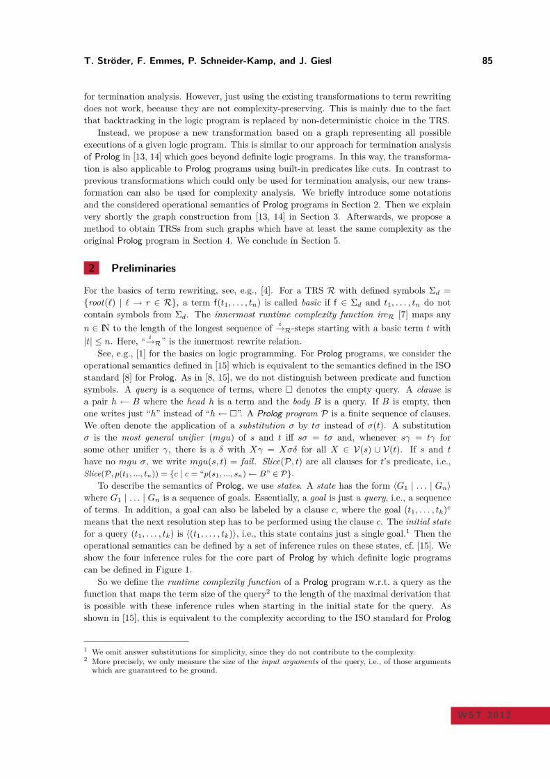
T. Ströder, F. Emmes, P. Schneider-Kamp, and J. Giesl 85
for termination analysis. However, just using the existing transformations to term rewriting
does not work, because they are not complexity-preserving. This is mainly due to the fact
that backtracking in the logic program is replaced by non-deterministic choice in the TRS.
Instead, we propose a new transformation based on a graph representing all possible
executions of a given logic program. This is similar to our approach for termination analysis
of Prolog in [13, 14] which goes beyond definite logic programs. In this way, the transforma-
tion is also applicable to Prolog programs using built-in predicates like cuts. In contrast to
previous transformations which could only be used for termination analysis, our new trans-
formation can also be used for complexity analysis. We briefly introduce some notations
and the considered operational semantics of Prolog programs in Section 2. Then we explain
very shortly the graph construction from [13, 14] in Section 3. Afterwards, we propose a
method to obtain TRSs from such graphs which have at least the same complexity as the
original Prolog program in Section 4. We conclude in Section 5.
2 Preliminaries
For the basics of term rewriting, see, e.g., [4]. For a TRS R with defined symbols Σd =
root(ℓ) | ℓ → r ∈ R, a term f(t1, . . . , tn) is called basic if f ∈ Σd and t1, . . . , tn do not
contain symbols from Σd. The innermost runtime complexity function ircR [7] maps any
n ∈ IN to the length of the longest sequence ofi→R-steps starting with a basic term t with
|t| ≤ n. Here, “i→R” is the innermost rewrite relation.
See, e.g., [1] for the basics on logic programming. For Prolog programs, we consider the
operational semantics defined in [15] which is equivalent to the semantics defined in the ISO
standard [8] for Prolog. As in [8, 15], we do not distinguish between predicate and function
symbols. A query is a sequence of terms, where denotes the empty query. A clause is
a pair h ← B where the head h is a term and the body B is a query. If B is empty, then
one writes just “h” instead of “h← ”. A Prolog program P is a finite sequence of clauses.
We often denote the application of a substitution σ by tσ instead of σ(t). A substitution
σ is the most general unifier (mgu) of s and t iff sσ = tσ and, whenever sγ = tγ for
some other unifier γ, there is a δ with Xγ = Xσδ for all X ∈ V(s) ∪ V(t). If s and t
have no mgu σ, we write mgu(s, t) = fail. Slice(P, t) are all clauses for t’s predicate, i.e.,
Slice(P, p(t1, ..., tn)) = c | c = “p(s1, ..., sn)← B” ∈ P.
To describe the semantics of Prolog, we use states. A state has the form 〈G1 | . . . | Gn〉
where G1 | . . . | Gn is a sequence of goals. Essentially, a goal is just a query, i.e., a sequence
of terms. In addition, a goal can also be labeled by a clause c, where the goal (t1, . . . , tk)c
means that the next resolution step has to be performed using the clause c. The initial state
for a query (t1, . . . , tk) is 〈(t1, . . . , tk)〉, i.e., this state contains just a single goal.1 Then the
operational semantics can be defined by a set of inference rules on these states, cf. [15]. We
show the four inference rules for the core part of Prolog by which definite logic programs
can be defined in Figure 1.
So we define the runtime complexity function of a Prolog program w.r.t. a query as the
function that maps the term size of the query2 to the length of the maximal derivation that
is possible with these inference rules when starting in the initial state for the query. As
shown in [15], this is equivalent to the complexity according to the ISO standard for Prolog
1 We omit answer substitutions for simplicity, since they do not contribute to the complexity.2 More precisely, we only measure the size of the input arguments of the query, i.e., of those arguments
which are guaranteed to be ground.
WST 2012
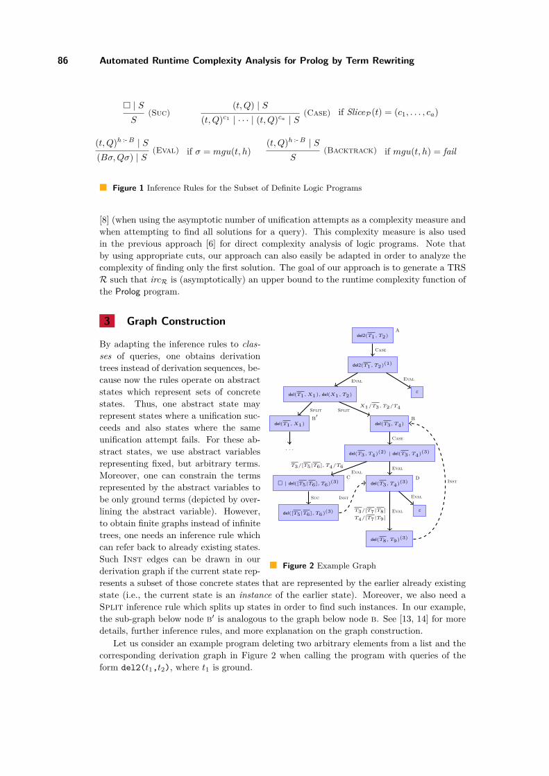
86 Automated Runtime Complexity Analysis for Prolog by Term Rewriting
| S
S(Suc)
(t, Q) | S
(t, Q)c1 | · · · | (t, Q)ca | S(Case) if SliceP(t) = (c1, . . . , ca)
(t, Q)h :-B | S
(Bσ,Qσ) | S(Eval) if σ = mgu(t, h)
(t, Q)h :-B | S
S(Backtrack) if mgu(t, h) = fail
Figure 1 Inference Rules for the Subset of Definite Logic Programs
[8] (when using the asymptotic number of unification attempts as a complexity measure and
when attempting to find all solutions for a query). This complexity measure is also used
in the previous approach [6] for direct complexity analysis of logic programs. Note that
by using appropriate cuts, our approach can also easily be adapted in order to analyze the
complexity of finding only the first solution. The goal of our approach is to generate a TRS
R such that ircR is (asymptotically) an upper bound to the runtime complexity function of
the Prolog program.
3 Graph Constructiondel2(T1, T2)
a
del2(T1, T2)(1)
Case
del(T1, X1), del(X1, T2)
Eval
ε
Eval
del(T3, T4)b
SplitX1/T3, T2/T4
del(T1, X1)b′
Split
. . .del(T3, T4)(2) | del(T3, T4)(3)
Case
| del([T5|T6], T6)(3)c
Eval
T3/[T5|T6], T4/T6
del(T3, T4)(3)d
Eval
del([T5|T6], T6)(3)
Suc Inst
del(T8, T9)(3)
EvalT3/[T7|T8]
T4/[T7|T9]
Inst
ε
Eval
Figure 2 Example Graph
By adapting the inference rules to clas-
ses of queries, one obtains derivation
trees instead of derivation sequences, be-
cause now the rules operate on abstract
states which represent sets of concrete
states. Thus, one abstract state may
represent states where a unification suc-
ceeds and also states where the same
unification attempt fails. For these ab-
stract states, we use abstract variables
representing fixed, but arbitrary terms.
Moreover, one can constrain the terms
represented by the abstract variables to
be only ground terms (depicted by over-
lining the abstract variable). However,
to obtain finite graphs instead of infinite
trees, one needs an inference rule which
can refer back to already existing states.
Such Inst edges can be drawn in our
derivation graph if the current state rep-
resents a subset of those concrete states that are represented by the earlier already existing
state (i.e., the current state is an instance of the earlier state). Moreover, we also need a
Split inference rule which splits up states in order to find such instances. In our example,
the sub-graph below node b′ is analogous to the graph below node b. See [13, 14] for more
details, further inference rules, and more explanation on the graph construction.
Let us consider an example program deleting two arbitrary elements from a list and the
corresponding derivation graph in Figure 2 when calling the program with queries of the
form del2(t1,t2), where t1 is ground.
T. Ströder, F. Emmes, P. Schneider-Kamp, and J. Giesl 87
(1) del2(XS, YS) :- del(XS, ZS), del(ZS, YS).
(2) del([X|XS], XS).
(3) del([X|XS], [X|YS]) :- del(XS, YS).
This program has quadratic complexity due to backtracking. However, if one encodes
the clauses directly as rules in a TRS, the backtracking is lost and we generate a TRS with
linear complexity. To obtain a transformation which over-approximates the complexity of
the original program (i.e., where the innermost runtime complexity of the resulting TRS is
an upper bound for the complexity of the Prolog program), we encode the paths of the graph
representation of the program, which explicitly represents the backtracking possibilities.
4 Synthesizing TRSs
To obtain TRSs from the graph, we consider the different successors of Split nodes sep-
arately. So in our example, we first generate a TRS from the graph that results from
removing the sub-graph with root node b and then we generate a TRS from the graph that
(essentially) results from removing the sub-graph with root node b′. Afterwards the runtime
complexities of these two TRSs are multiplied in order to obtain an upper bound for the
runtime complexity of the original logic program. The reason is that due to backtracking,
every solution for the query in the leftmost Split child triggers an evaluation of the query
in the rightmost Split child.
To generate TRSs from graphs, we encode each state s by two fresh function symbols
f ins
and fouts
. The arguments of f ins
are the (ground) input arguments of s and for fouts
, we
use the output arguments of s that are guaranteed to be ground after evaluating the query
in s. (To detect those arguments, we use a groundness analysis for the logic program.)
We generate rewrite rules for the paths that start in the initial node of the graph or in a
successor state of an Inst or Split node and that end in a Suc node or in a successor of an
Inst or Split node. Moreover, except for the first and last node of the path, the path may
not traverse successors of Inst or Split nodes. In our example we obtain a TRS R1 for
the graph where we disregard the subgraph with root node b and a TRS R2 for the graph
where we disregard the subgraph with root node b′. So in R2 we obtain rules for the paths
from a to b (Rule (1)), b to c (Rule (2)), b to d directly (Rule (3)), b to d via c (Rule (4)),
and d to b (Rule (5)). We always apply all substitutions along the path to the left-hand
side of the resulting rewrite rule. See [12] for more details on how to encode clauses as rules
in a TRS. Moreover, the rule from a to b has to take into account that the input argument
T3 of b is the result of evaluating b′. Thus, when computing the complexity of R2, we can
also use the rules of R1 for evaluating terms, but these evaluations do not contribute to the
complexity of R2. Such notions of complexity have already been used in existing frameworks
for complexity analysis of TRSs [7, 10, 18]. For space reasons, here we only present R2. The
TRS R1 is analogous to R2 except for R1’s first rule which is f ina (T1)→ f inb′ (T1).
f ina (T1) → f inb (T3) | f ina (T1) →∗ foutb′ (T3) (1)
f inb ([T5 | T6]) → foutb (T6) (2)
f inb (T3) → foutb (T4) | f ind (T3) →∗ foutd (T4) (3)
f inb ([T5 | T6]) → foutb (T6) | f ind ([T5 | T6]) →∗ foutd (T6) (4)
f ind ([T7 | T8]) → foutd ([T7 | T9]) | f inb (T8) →∗ foutb (T9) (5)
To analyze these conditional TRSs for complexity, they are first transformed into uncon-
ditional TRSs using a standard transformation, cf. e.g., [11]. In our example, the resulting
WST 2012
88 Automated Runtime Complexity Analysis for Prolog by Term Rewriting
complexities of R1 and R2 are both linear. Since their complexities have to be multiplied
due to backtracking, this yields a quadratic upper bound for our example logic program.
5 Conclusion
We proposed a new method for automated complexity analysis of Prolog programs based
on automated complexity analysis of term rewriting. First experiments with a prototype
implementation have shown promising results. The next steps for this approach are formal
definitions and proofs of correctness, a complete implementation, and a thorough experi-
mental evaluation.
References
1 K. R. Apt. From Logic Programming to Prolog. Prentice Hall, 1997.
2 M. Avanzini, G. Moser, and A. Schnabl. Automated implicit computational complexity
analysis. In IJCAR ’08, LNAI 5195, pages 132–138, 2008.
3 M. Avanzini and G. Moser. Dependency pairs and polynomial path orders. In RTA ’09,
LNCS 5595, pages 48–62, 2009.
4 F. Baader and T. Nipkow. Term Rewriting and All That. Cambridge University Press,
1998.
5 G. Bonfante, A. Cichon, J.-Y. Marion, and H. Touzet. Algorithms with polynomial inter-
pretation termination proof. Journal of Functional Programming, 11(1):33–53, 2001.
6 S. K. Debray and N.-W. Lin. Cost analysis of logic programs. ACM Transactions on
Programming Languages and Systems, 15:826–875, 1993.
7 N. Hirokawa and G. Moser. Automated complexity analysis based on the dependency pair
method. In IJCAR ’08, LNAI 5195, pages 364–379, 2008.
8 ISO/IEC 13211-1. Information technology - Programming languages - Prolog. 1995.
9 J.-Y. Marion and R. Péchoux. Characterizations of polynomial complexity classes with a
better intensionality. In PPDP ’08, pages 79–88. ACM Press, 2008.
10 L. Noschinski, F. Emmes, J. Giesl. The dependency pair framework for automated com-
plexity analysis of term rewrite systems. In CADE ’11, LNAI 6803, pages 422–438, 2011.
11 E. Ohlebusch. Termination of Logic Programs: Transformational Methods Revisited. Ap-
plicable Algebra in Engineering, Communication and Computing, 12(1–2):73–116, 2001.
12 P. Schneider-Kamp, J. Giesl, A. Serebrenik, and R. Thiemann. Automated Termination
Proofs for Logic Programs by Term Rewriting. ACM Transactions on Computational Logic,
10(1), 2009.
13 P. Schneider-Kamp, J. Giesl, T. Ströder, A. Serebrenik, and R. Thiemann. Automated
termination analysis for logic programs with cut. In ICLP ’10, Theory and Practice of
Logic Programming, 10(4-6):365–381, 2010.
14 T. Ströder, P. Schneider-Kamp, J. Giesl. Dependency Triples for Improving Termination
Analysis of Logic Programs with Cut. In LOPSTR ’10, LNCS 6564, pages 184–199, 2011.
15 T. Ströder, F. Emmes, P. Schneider-Kamp, J. Giesl, and C. Fuhs. A linear operational
semantics for termination and complexity analysis of ISO Prolog. In LOPSTR ’11, 2011.
To appear.
16 The Termination Competition.
http://www.termination-portal.org/wiki/Termination_Competition.
17 J. Waldmann. Polynomially bounded matrix interpretations. In RTA ’10, LIPIcs 6, pages
357–372, 2010.
18 H. Zankl and M. Korp. Modular complexity analysis via relative complexity. In RTA ’10,
LIPIcs 6, pages 385–400, 2010.
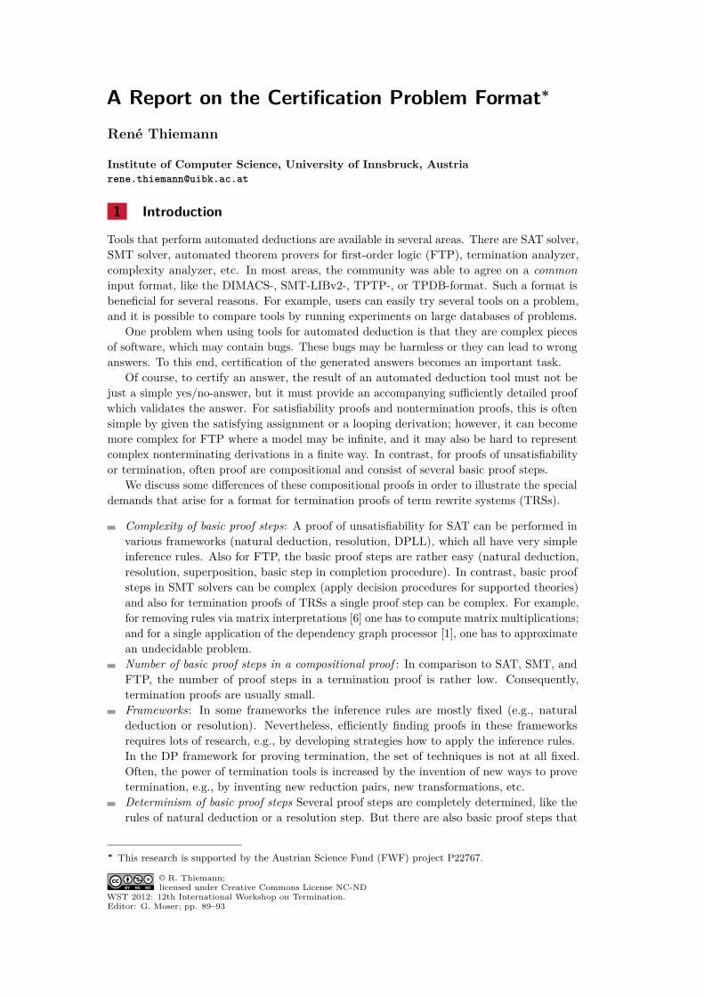
A Report on the Certification Problem Format∗
René Thiemann
Institute of Computer Science, University of Innsbruck, Austria
1 Introduction
Tools that perform automated deductions are available in several areas. There are SAT solver,SMT solver, automated theorem provers for first-order logic (FTP), termination analyzer,complexity analyzer, etc. In most areas, the community was able to agree on a common
input format, like the DIMACS-, SMT-LIBv2-, TPTP-, or TPDB-format. Such a format isbeneficial for several reasons. For example, users can easily try several tools on a problem,and it is possible to compare tools by running experiments on large databases of problems.
One problem when using tools for automated deduction is that they are complex piecesof software, which may contain bugs. These bugs may be harmless or they can lead to wronganswers. To this end, certification of the generated answers becomes an important task.
Of course, to certify an answer, the result of an automated deduction tool must not bejust a simple yes/no-answer, but it must provide an accompanying sufficiently detailed proofwhich validates the answer. For satisfiability proofs and nontermination proofs, this is oftensimple by given the satisfying assignment or a looping derivation; however, it can becomemore complex for FTP where a model may be infinite, and it may also be hard to representcomplex nonterminating derivations in a finite way. In contrast, for proofs of unsatisfiabilityor termination, often proof are compositional and consist of several basic proof steps.
We discuss some differences of these compositional proofs in order to illustrate the specialdemands that arise for a format for termination proofs of term rewrite systems (TRSs).
Complexity of basic proof steps: A proof of unsatisfiability for SAT can be performed invarious frameworks (natural deduction, resolution, DPLL), which all have very simpleinference rules. Also for FTP, the basic proof steps are rather easy (natural deduction,resolution, superposition, basic step in completion procedure). In contrast, basic proofsteps in SMT solvers can be complex (apply decision procedures for supported theories)and also for termination proofs of TRSs a single proof step can be complex. For example,for removing rules via matrix interpretations [6] one has to compute matrix multiplications;and for a single application of the dependency graph processor [1], one has to approximatean undecidable problem.Number of basic proof steps in a compositional proof : In comparison to SAT, SMT, andFTP, the number of proof steps in a termination proof is rather low. Consequently,termination proofs are usually small.Frameworks: In some frameworks the inference rules are mostly fixed (e.g., naturaldeduction or resolution). Nevertheless, efficiently finding proofs in these frameworksrequires lots of research, e.g., by developing strategies how to apply the inference rules.In the DP framework for proving termination, the set of techniques is not at all fixed.Often, the power of termination tools is increased by the invention of new ways to provetermination, e.g., by inventing new reduction pairs, new transformations, etc.Determinism of basic proof steps Several proof steps are completely determined, like therules of natural deduction or a resolution step. But there are also basic proof steps that
∗ This research is supported by the Austrian Science Fund (FWF) project P22767.
© R. Thiemann;
licensed under Creative Commons License NC-ND
WST 2012: 12th International Workshop on Termination.
Editor: G. Moser; pp. 89–93

90 A Report on the Certification Problem Format
tool 1
tool 2
tool 3
...
human readable
Rainbow output
CiME3 output
CeTA output
Rainbow/CoLoR
CiME3/Coccinelle
CeTA/IsaFoR
Figure 1 Certification of termination proofs before CPF
need further information to determine the result. For example, from one conflict in DPLLone can learn different conflict clauses; and for an application of the dependency graphprocessor, the result depends on the used approximation.
To summarize, termination proofs are usually small, but each basic proof step is complex.Moreover, the set of applied termination techniques is constantly growing.
In this report, we shortly present the certification problem format (CPF), a formatdeveloped to represent termination proofs. It has four major benefits. First, it is easy fortermination tools to generate CPF files; second, it is easy to add new techniques to CPF;third, it provides enough information for certification; finally, it is a common proof formatthat is supported by several tools and certifiers.
All details on CPF and several example proofs are freely available at the following URL.
http://cl-informatik.uibk.ac.at/software/cpf/
2 The Certification Problem Format
Before any certifiers for termination proofs have been developed, each termination tool forTRSs provided proofs in a human-readable HTML or plain text file. From these files it washard to extract the relevant proof steps since parameters of termination techniques are mixedwith human readable explanations. Moreover, the output was not standardized at all, butevery tool produced proofs in its own output format.
Hence, when the first certifiers for termination proofs have been developed (Rainbow/CoLoR
[2], CiME3/Coccinelle [4], and later CeTA/IsaFoR [19]), each of the certifiers demanded a proofwritten in their own format as input. Hence, to support certifiable proofs using all certifiers,a termination tool had to write several proof routines output, as illustrated in Figure 1.
To reduce the number of required proof outputs for termination tools, the three groups ofthe certifiers decided to develop one proof format that should be supported by all certifiers,namely CPF. Therefore, for generation of certifiable proofs, termination tools now only haveto support CPF output. As CPF was also developed with several feedbacks from varioustermination tools it is widely accepted in the community and it is currently used as the onlyformat during the termination competition for certified categories.
CPF is an XML-format. Choosing XML instead of ASCII was possible as terminationproofs are rather small. So, the additional size-overhead of XML documents does not playsuch a crucial role as it might have played for (large) unsatisfiability proofs for SAT or SMT.
Using XML has several advantages: it is easy to generate, since often programminglanguages directly offer libraries for XML processing; even before certifiers can check thegenerated proofs, one can use standard XML programs to check whether a CPF file respectsthe required XML structure; and finally, it was easy to write a pretty printer to obtain
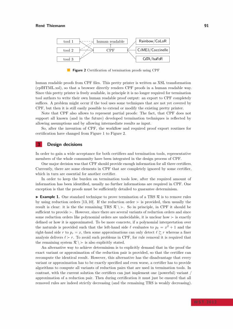
René Thiemann 91
tool 1
tool 2
tool 3
human readable
CPF
Rainbow/CoLoR
CiME3/Coccinelle
CeTA/IsaFoR
Figure 2 Certification of termination proofs using CPF
human readable proofs from CPF files. This pretty printer is written as XSL transformation(cpfHTML.xsl), so that a browser directly renders CPF proofs in a human readable way.Since this pretty printer is freely available, in principle it is no longer required for terminationtool authors to write their own human readable proof output: an export to CPF completelysuffices. A problem might occur if the tool uses some techniques that are not yet covered byCPF, but then it is still easily possible to extend or modify the existing pretty printer.
Note that CPF also allows to represent partial proofs: The fact, that CPF does notsupport all known (and in the future) developed termination techniques is reflected byallowing assumptions and by allowing intermediate results as input.
So, after the invention of CPF, the workflow and required proof export routines forcertification have changed from Figure 1 to Figure 2.
3 Design decisions
In order to gain a wide acceptance for both certifiers and termination tools, representativemembers of the whole community have been integrated in the design process of CPF.
One major decision was that CPF should provide enough information for all three certifiers.Currently, there are some elements in CPF that are completely ignored by some certifier,which in turn are essential for another certifier.
In order to keep the burden on termination tools low, after the required amount ofinformation has been identified, usually no further informations are required in CPF. Oneexception is that the proofs must be sufficiently detailed to guarantee determinism.
Example 1. One standard technique to prove termination of a TRS R is to remove rulesby using reduction orders [13, 10]. If the reduction order ≻ is provided, then usually theresult is clear: it is the the remaining TRS R \ ≻. So in principle, in CPF it should besufficient to provide ≻. However, since there are several variants of reduction orders and sincesome reduction orders like polynomial orders are undecidable, it is unclear how ≻ is exactlydefined or how it is approximated. To be more concrete, if a polynomial interpretation overthe naturals is provided such that the left-hand side ℓ evaluates to pℓ = x2 + 1 and theright-hand side r to pr = x, then some approximations can only detect ℓ % r whereas a fineranalysis delivers ℓ ≻ r. To avoid such problems in CPF, for rule removal it is required thatthe remaining system R \ ≻ is also explicitly stated.
An alternative way to achieve determinism is to explicitly demand that in the proof theexact variant or approximation of the reduction pair is provided, so that the certifier canrecompute the identical result. However, this alternative has the disadvantage that everyvariant or approximation has to be exactly specified and even worse, a certifier has to providealgorithms to compute all variants of reduction pairs that are used in termination tools. Incontrast, with the current solution the certifiers can just implement one (powerful) variant /approximation of a reduction pair. Then during certification it must just be ensured that allremoved rules are indeed strictly decreasing (and the remaining TRS is weakly decreasing).
WST 2012
92 A Report on the Certification Problem Format
Note that determinism of each proof step is also important for an early detection of errors.Otherwise, it might happen that a difference in the internal proof state of the terminationtool and the state in the certifier remains undetected for several proof steps. And then errorsare reported in proof steps which are perfectly okay.
Example 2. Let R = f(s(x))→ f(t(x)), g(x)→ g(s(x)). Consider a wrong proof wherefirst the polynomial order with Pol(h(x)) = x for all h ∈ f, g, s, t is used to remove the ruleg(x) → g(s(x)); second, the only dependency pair f♯(s(x)) → f♯(t(x)) is generated; finally,termination is proven since the dependency graph contains no edges.
If during the certification one just applies the same techniques without checking theintermediate results, then one first applies rule removal without removing any rule; second,one computes the dependency pairs including g♯(x) → g♯(s(x)); and finally, the error isreported that the dependency graph is not empty. Hence, the error in the first step is notdetected, but in the final step—although the final step in the termination tool is sound.
Minor design decisions had to be made for all supported techniques,1 e.g., the exact namesand the exact representation of the relevant parameters, etc. For these decisions, usually theperson who wanted to add a new technique to CPF was asked to provide a proposal. Thisproposal was then integrated into a development version of CPF and put under discussion onthe CPF mailing list. Comments during the discussion were integrated in the proposal, andafter the discussion has stopped, the modified proposal was then integrated into the officialCPF version.
4 Problems and Future of CPF
Very recently, other classes than termination proofs were added to CPF, namely confluenceproofs, completion proofs (is a TRS convergent and equivalent to an equational theory?),and equational proofs. Especially for completion proofs, the size of CPF files has growntremendously. In experiments, example proofs of over 400 megabytes have been generated.2
For these large proofs, both the completion tool and the certifier spend most of their timefor proof export or parsing of XML documents.
Hence, action is required to counter the size-overhead of XML documents. Possibilitieswould include indexing of terms and rules. Moreover, for rule removal techniques, onemight change CPF in such a way that the removed rules have to be provided instead of theremaining rules.3 The latter change would also allow to represent the rule removal techniquesfor termination and relative termination in the same way, which in turn would allow to mergethe proof techniques for termination and relative termination.
1 Currently CPF supports several classes of reduction pairs (in alphabetical order): argument filters [1],matrix orders [6], polynomial orders over several carriers [13, 12, 15], recursive path orders [5], andSCNP reduction pairs [3]. Moreover, the techniques of dependency graph [1], dependency pairs [1, 8],dependency pair transformations [1, 8], loops, matchbounds [7], root labeling [16], rule removal [13, 10],semantic labeling [21], size-change termination [14, 18], string reversal, subterm criterion [10], switchingto innermost termination [9], uncurrying [11,17], and usable rules[1, 20,8] are supported.
2 We mention a completion proof for an example with 4 equations and 11 rules in the completed TRS.In this proof, only to show that all rules in the TRS can be derived from the equations, ≈ 90, 000reductions have been performed, and the accumulated terms in these derivations consists of over 5million function symbols and variables. Since symbols are strings and since there is the XML-overhead,in total, one obtains a 406 MB file (converting all symbols to integers still results in a 266 MB file).CeTA spend only 1 % of its time for checking the proof, and 99 % for parsing.
3 If the remaining system has to specified, several steps of removing a single rule require quadratic size,whereas if one specifies the removed rules, then the size of the overall proof is linear.
René Thiemann 93
However, these changes would be non-conservative changes which requires adaptations ofthe proof generating tools and the certifiers. Therefore, we believe that it should be discussedthoroughly by the community whether such changes should be made. Everyone is invited tocontribute in the discussion.
References
1 T. Arts and J. Giesl. Termination of term rewriting using dependency pairs. Theoretical
Computer Science, 236(1-2):133–178, 2000.2 F. Blanqui and A. Koprowski. CoLoR: a Coq library on well-founded rewrite relations
and its application on the automated verification of termination certificates. Mathematical
Structures in Computer Science, 21(4):827–859, 2011.3 M. Codish, C. Fuhs, J. Giesl, and P. Schneider-Kamp. Lazy abstraction for size-change
termination. In Proc. LPAR ’10, volume 6397 of LNCS, pages 217–232, 2010.4 É. Contejean, P. Courtieu, J. Forest, O. Pons, and X. Urbain. Automated certified proofs
with CiME3 3. In Proc. RTA ’11, volume 10 of LIPIcs, pages 21–30. 2011.5 N. Dershowitz. Termination of rewriting. J. Symb. Comp., 3(1-2):69–116, 1987.6 J. Endrullis, J. Waldmann, and H. Zantema. Matrix interpretations for proving termination
of term rewriting. Journal of Automated Reasoning, 40(2-3):195–220, 2008.7 A. Geser, D. Hofbauer, J. Waldmann, and H. Zantema. On Tree Automata that Certify
Termination of Left-Linear Term Rewriting Systems. Inf. & Comp., 205(4):512–534, 2007.8 J. Giesl, R. Thiemann, P. Schneider-Kamp, and S. Falke. Mechanizing and improving
dependency pairs. Journal of Automated Reasoning, 37(3):155–203, 2006.9 B. Gramlich. Abstract relations between restricted termination and confluence properties
of rewrite systems. Fundamenta Informaticae, 24:3–23, 1995.10 N. Hirokawa and A. Middeldorp. Tyrolean Termination Tool: Techniques and features. Inf.
& Comp., 205(4):474–511, 2007.11 N. Hirokawa, A. Middeldorp, and H. Zankl. Uncurrying for termination. In Proc. LPAR’08,
volume 5330 of LNAI, pages 667–681. 2008.12 A. Koprowski and J. Waldmann. Arctic termination . . . below zero. In Proc. RTA’08,
volume 5117 of LNCS, pages 202–216, 2008.13 D. Lankford. On proving term rewriting systems are Noetherian. Technical Report MTP-3,
Louisiana Technical University, Ruston, LA, USA, 1979.14 C. S. Lee, N. D. Jones, and A. M. Ben-Amram. The size-change principle for program
termination. In Proc. POPL ’01, pages 81–92, 2001.15 S. Lucas. Polynomials over the reals in proofs of termination: From theory to practice.
RAIRO – Theoretical Informatics and Applications, 39(3):547–586, 2005.16 C. Sternagel and A. Middeldorp. Root-Labeling. In RTA’08, volume 5117 of LNCS, pages
336–350. 2008.17 C. Sternagel and R. Thiemann. Generalized and formalized uncurrying. In Proc. FroCoS’11,
volume 6989 of LNAI, pages 243–258. 2011.18 R. Thiemann and J. Giesl. The size-change principle and dependency pairs for termination
of term rewriting. Appl. Alg. Eng. Comm. Comput., 16(4):229–270, 2005.19 R. Thiemann and C. Sternagel. Certification of termination proofs using CeTA. In
TPHOLs’09, volume 5674 of LNCS, pages 452–468. 2009.20 X. Urbain. Automated incremental termination proofs for hierarchically defined term rewrit-
ing systems. In Proc. IJCAR 2001, volume LNAI 2083, pages 485–498, 2001.21 H. Zantema. Termination of term rewriting by semantic labelling. Fundamenta Informati-
cae, 24:89–105, 1995.
WST 2012
Automating Ordinal Interpretations
Harald Zankl, Sarah Winkler∗, and Aart Middeldorp
Institute of Computer Science, University of Innsbruck, Austria
Abstract
In this note we study weakly monotone interpretations for direct proofs of termination which is
sound if the interpretation functions are “simple”. This is e.g. the case for standard addition and
multiplication of ordinal numbers. We compare the power of such interpretations to polynomial
interpretations over the natural numbers and report on preliminary experimental results.
1 Introduction
Polynomial interpretations [9] are a well-established termination technique. By now powerful
techniques are known for their automation [1, 5]. Recently it has been shown that allowing
different domains, (e.g., N, Q, R) results in incomparable termination criteria [11,14]. Matrix
interpretations consider linear interpretations over vectors or matrices of numbers (in N, Q,
R) and have been shown to be powerful in theory and practice [2,6,4,18]. However, for other
extensions (e.g., elementary functions [10, 12] or interpretations into ordinal numbers [16])
practical implementations remain an open problem.
In this note we revisit polynomial interpretations using ordinals as carrier [16]. Based on
recent results [17], we present an implementation for string rewrite systems (with interpreta-
tion functions of a special shape), which is the first one to our knowledge. Our efforts could
be seen as a first step towards automatically proving the battle of Hercules and Hydra [16]
terminating. However—for the encoding of the battle from [3]—Moser [13, Section 7] antic-
ipates that an extension of polynomial interpretations into ordinal domains is not sufficient.
In the remainder of this introductory section we recall preliminaries.
Ordinals: We assume basic knowledge of ordinals [8]. By O we denote the set of ordinal
numbers strictly less than ǫ0. Every ordinal α ∈ O has a unique representation in Cantor
Normal Form (CNF): α =∑
16i6n ωαi · ai, where a1, . . . , an ∈ N \ 0 and α1, . . . , αn ∈ O
are also in CNF, with α > α1 > · · · > αn. We denote standard addition and multiplication
on O (and hence also on N) by + and ·. We furthermore drop · whenever convenient.
Term Rewriting: We assume familiarity with term rewriting and termination [15]. Let >
be a relation and > its reflexive closure. A function f is monotone if a > b implies
f(. . . , a, . . .) > f(. . . , b, . . .) and weakly monotone if a > b implies f(. . . , a, . . .) > f(. . . , b, . . .).
A function f is simple if f(. . . , a, . . .) > a.
An F-algebra A consists of a carrier set A and an interpretation function fA : Ak → A
for each k-ary function symbol f ∈ F . By [α]A(·) we denote the usual evaluation function of
A according to an assignment α which maps variables to values in A. An F-algebra together
with a well-founded order > on A is called a (well-founded) F-algebra (A, >). Often we
denote (A, >) by A if > is clear from the context. The order > induces a well-founded order
on terms: s >A t if and only if [α]A(s) > [α]A(t) for all assignments α. A TRS R and
an algebra A are compatible if ℓ >A r for all ℓ → r ∈ R. A well-founded algebra (A, >)
is a monotone (weakly monotone / simple) algebra if for every function symbol f ∈ F the
interpretation function fA is monotone (weakly monotone / simple) in all arguments. By O
(N ) we denote well-founded algebras with the carrier O (N) and the standard order >.
∗ Supported by a DOC-fFORTE fellowship of the Austrian Academy of Sciences.
© H. Zankl, S. Winkler, and A. Middeldorp;
licensed under Creative Commons License NC-ND
WST 2012: 12th International Workshop on Termination.
Editor: G. Moser; pp. 94–98
H. Zankl, S. Winkler, and A. Middeldorp 95
For (direct) termination proofs one typically exploits the following theorem.
Theorem 1.1. A TRS is terminating if and only if it is compatible with a well-founded
monotone algebra.
However, monotonicity can be replaced by weak monotonicity, provided the interpreta-
tion functions are simple. This result is less known.
Theorem 1.2 ([19, Proposition 12]). A TRS is terminating if it is compatible with a
well-founded weakly monotone simple algebra.
2 Ordinal Interpretations
Although standard addition, multiplication and exponentiation on ordinals are in general
only weakly monotone, Theorem 1.2 nevertheless constitutes a way to use interpretations
into the ordinals with these operations in termination proofs.
The next example shows that (fairly small) ordinals add power to linear interpretations.
Example 2.1. Consider the SRS R consisting of the rule a(b(x))→ b(a(a(x))). The linear
ordinal interpretation
aO(x) = x+ 1 bO(x) = x+ ω
is simple and proves termination of R since x + ω + 1 >O x + 1 + 1 + ω = x + ω. Linear
interpretations with coefficients in N are not sufficient. Assuming abstract interpretations
aN (x) = a1x+ a0 and bN (x) = b1x+ b0, we obtain the constraints
a1b1 > b1a1a1 a1b0 + a0 > b1a1a0 + b1a0 + b0
Since aN and bN must be simple (or monotone) a1, b1 > 1. From the first constraint we
conclude a1 = 1, which makes the second one unsatisfiable.
In the rest of this note we consider ordinal interpretations (for SRSs) of the following
shape
fO(x) = x · f ′ + ωd · fd + · · ·+ ω1 · f1 + f0 (1)
where f ′, fd, . . . , f0 ∈ N. Interpretations of the shape (1) will be called linear ordinal in-
terpretations (of degree d). Note that interpretations of the shape (1) are weakly monotone
and simple if f ′ > 1. To show the power of linear ordinal interpretations (with respect to
the derivational complexity) we define the parametrized SRS Rm.
Definition 2.2. For any m ∈ N the SRS Rm consists of the rules
ai(ai+1(x))→ ai+1(ai(ai(x))) ai+1(x)→ x
for each 0 6 i < m.
Note that R0 is empty. We have the following properties.
Lemma 2.3. For any Rm and i 6 m we have ai(an
i+1(x))→2n−1 ani+1(a2n
i(x)).
Proof. By induction on n. In the base case n = 0 and ai(x)→0 ai(x). In the step case
ai(an+1i+1 (x))→ ai+1(ai(ai(a
n
i+1(x))))→2n−1 ai+1(ai(an
i+1(a2n
i(x))))
→2n−1 ai+1(ani+1(a2n
i(a2n
i(x)))) = an+1
i+1 (a2n+1
i(x))
WST 2012
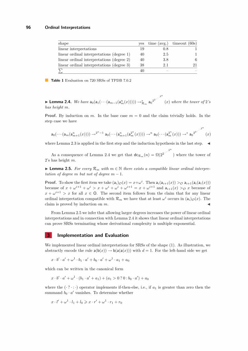
96 Ordinal Interpretations
shape yes time (avg.) timeout (60s)
linear interpretations 19 0.8 1
linear ordinal interpretations (degree 1) 40 2.5 1
linear ordinal interpretations (degree 2) 40 3.8 6
linear ordinal interpretations (degree 3) 38 2.1 21∑
40 – –
Table 1 Evaluation on 720 SRSs of TPDB 7.0.2
Lemma 2.4. We have a0(a1(· · · (am−1(anm
(x)))))→∗Rm a022 ·
·
·
2n
(x) where the tower of 2’s
has height m.
Proof. By induction on m. In the base case m = 0 and the claim trivially holds. In the
step case we have
a0(· · · (am(anm+1(x))))→2n−1 a0(· · · (an
m+1(a2n
m(x))))→n a0(· · · (a2n
m(x)))→∗ a0
22 ··
·
2n
(x)
where Lemma 2.3 is applied in the first step and the induction hypothesis in the last step.
As a consequence of Lemma 2.4 we get that dcRm(n) = Ω(22 ··
·
2n
) where the tower of
2’s has height m.
Lemma 2.5. For every Rm with m ∈ N there exists a compatible linear ordinal interpre-
tation of degree m but not of degree m− 1.
Proof. To show the first item we take (ai)O(x) = x+ωi. Then ai(ai+1(x)) >O ai+1(ai(ai(x)))
because of x + ωi+1 + ωi > x + ωi + ωi + ωi+1 = x + ωi+1 and ai+1(x) >O x because of
x + ωi+1 > x for all x ∈ O. The second item follows from the claim that for any linear
ordinal interpretation compatible with Rm we have that at least ωi occurs in (ai)O(x). The
claim is proved by induction on m.
From Lemma 2.5 we infer that allowing larger degrees increases the power of linear ordinal
interpretations and in connection with Lemma 2.4 it shows that linear ordinal interpretations
can prove SRSs terminating whose derivational complexity is multiple exponential.
3 Implementation and Evaluation
We implemented linear ordinal interpretations for SRSs of the shape (1). As illustration, we
abstractly encode the rule a(b(x))→ b(a(a(x))) with d = 1. For the left-hand side we get
x · b′ · a′ + ω1 · b1 · a′ + b0 · a
′ + ω1 · a1 + a0
which can be written in the canonical form
x · b′ · a′ + ω1 · (b1 · a′ + a1) + (a1 > 0 ? 0 : b0 · a
′) + a0
where the (· ? · : ·) operator implements if-then-else, i.e., if a1 is greater than zero then the
summand b0 · a′ vanishes. To determine whether
x · l′ + ω1 · l1 + l0 > x · r′ + ω1 · r1 + r0
H. Zankl, S. Winkler, and A. Middeldorp 97
for all values of x, we use the criterion l′ > r′ ∧ (l1 > r1 ∨ (l1 = r1 ∧ l0 > r0)). Finally,
f ′ > 1 ensures that the interpretation fO is simple while the interpretation functions are
then weakly monotone for free. Hence the search for suitable coefficients can be encoded in
non-linear integer arithmetic.
The results1 are given in Table 1 where 4 bits are used to represent the coefficients
f0, . . . , fn, f′ and 8 bits are allowed for intermediate calculations. The column labeled “yes”
indicates how many systems the given method could show terminating. Times are given in
seconds.
4 Conclusion
We conclude this note with a short discussion on the relationship of linear ordinal inter-
pretations with matrix interpretations [4]. In contrast to the latter the induced ordering
is still total which makes it valuable for ordered completion. Secondly as Lemmata 2.4
and 2.5 show interpretations of the shape (1) allow to prove termination of SRSs whose
derivational complexity is beyond exponential while matrix interpretations are restricted to
an exponential upper bound.
Concerning future work we want to investigate if and how Theorem 1.2 could make
automated termination and complexity tools more powerful.
For matrix interpretations over N (as defined in [4]) the answer is that Theorem 1.2 does
not increase the power of the method. The reason is that the condition for a function to be
simple (Mii > 1 for all 1 6 i 6 d where d is the dimension of the matrices) is a stronger
requirement than monotonicity demanding M11 > 1.
However, if one considers matrix interpretations over O then additional termination
proofs can be obtained (note that any linear ordinal interpretation corresponds to a matrix
interpretation over O).
Another natural question is whether Theorem 1.2 helps arctic interpretations. Because
of monotonicity requirements, direct proofs with arctic matrices are currently limited to
dummy systems (SRSs augmented with constants).
Finally we recall that Theorem 1.2 allows direct proofs with polynomial interpretations
augmented with “max”. This has already been observed in [19, example on p. 13] but seems
to have been forgotten. A similar statement holds for quasi-periodic functions [20].
As future work we want to consider linear ordinal interpretations for TRSs. The problem
for TRSs is that for comparisons of polynomials the absolute positiveness approach [7] might
not apply. To see this note that f1 > g1 and f2 > g2 does not imply x·f1+y ·f2 > y ·g2+x·g1for all values of x and y if f1, f2, g1, g2 ∈ N and x, y ∈ O. To also cope with such cases we
propose a combination of standard and natural operations on ordinals, as illustrated in the
following example, where ⊕ denotes natural addition on O.
Example 4.1 (Adapted from [17, Example 17]). Consider the TRS R consisting of the
single rule s(f(x, y)) → f(s(y), s(s(x))). The weakly monotone interpretation fO(x, y) =
(x ⊕ y) + ω and sO(x) = x + 1 is simple and induces a strict decrease between left- and
right-hand side:
(x⊕ y) + ω + 1 >O ((y + 1)⊕ (x+ 2)) + ω = (x⊕ y) + 3 + ω = (x⊕ y) + ω
1 Details are available from http://colo6-c703.uibk.ac.at/ttt2/tpoly/.
WST 2012
98 Ordinal Interpretations
Hence R can be oriented by a linear ordinal interpretation. Again, linear interpretations
with coefficients in N are not sufficient. Assuming abstract interpretations fN (x, y) = f1x+
f2y + f0 and sN (x) = s1x+ s0, we get the constraints
s1f1 > f2s1s1 s1f2 > f1s1 s1f0 + s0 > f1s0 + f2(s0 + s1s0) + f0
Since sN and fN must be simple (or monotone) s1, f1, f2 > 1. From the first two constraints
we conclude s1 = 1, such that the third simplifies to f0 + s0 > f0 + (f1 + 2f2)s0. This
contradicts f1 and f2 being positive.
Acknowledgments: We thank Bertram Felgenhauer and the reviewers for useful comments.
References
1 Contejean, E., Marché, C., Tomás, A.P., Urbain, X.: Mechanically proving termination
using polynomial interpretations. JAR 34(4), 325–363 (2005)
2 Courtieu, P., Gbedo, G., Pons, O.: Improved matrix interpretations. In: SOFSEM 2009.
LNCS, vol. 5901, pp. 283–295 (2009)
3 Dershowitz, N., Jouannaud, J.P. In: Rewrite Systems. Handbook of Theoretical Computer
Science. vol. B: Formal Models and Sematics. (1990) 243–320
4 Endrullis, J., Waldmann, J., Zantema, H.: Matrix interpretations for proving termination
of term rewriting. JAR 40(2-3), 195–220 (2008)
5 Fuhs, C., Giesl, J., Middeldorp, A., Schneider-Kamp, P., Thiemann, R., Zankl, H.: SAT
solving for termination analysis with polynomial interpretations. In: SAT 2007. LNCS, vol.
4501, pp. 340–354 (2007)
6 Hofbauer, D., Waldmann, J.: Termination of string rewriting with matrix interpretations.
In: RTA 2006. LNCS, vol. 4098, pp. 328–342 (2006)
7 Hong, H., Jakuš, D.: Testing positiveness of polynomials. JAR 21(1), 23–38 (1998)
8 Jech, T.: Set Theory. Springer, Heidelberg (2002)
9 Lankford, D.: On proving term rewrite systems are noetherian. Technical Report MTP-3,
Louisiana Technical University, Ruston, LA, USA (1979)
10 Lescanne, P.: Termination of rewrite systems by elementary interpretations. Formal Asp.
Comp. 7(1), 77–90 (1995)
11 Lucas, S.: On the relative power of polynomials with real, rational, and integer coefficients
in proofs of termination of rewriting. AAECC 17(1), 49–73 (2006)
12 Lucas, S.: Automatic proofs of termination with elementary interpretations. ENTCS
258(1), 41–61 (2009)
13 Moser, G.: The Hydra battle and Cichon’s principle. AAECC 20(2), 133–158 (2009)
14 Neuratuer, F., Middeldorp, A.: Polynomial interpretations over the reals do not subsume
polynomial interpretations over the integers. In: RTA 2010. LIPIcs, vol. 6, pp. 243–258
(2010)
15 TeReSe: Term Rewriting Systems. vol. 55 of Cambridge Tracts in Theoretical Computer
Science. Cambridge University Press (2003)
16 Touzet, H.: Encoding the Hydra battle as a rewrite system. In: MFCS 1998. LNCS, vol.
1450, pp. 267–276 (1998)
17 Winkler, S., Zankl, H., Middeldorp, A.: Ordinals and Knuth-Bendix orders. In: LPAR-18.
LNCS (ARCoSS), vol. 7180, pp. 420–434 (2012)
18 Zankl, H., Middeldorp, A.: Satisfiability of non-linear (ir)rational arithmetic. In: LPAR-16.
LNCS (LNAI), vol. 6355, pp. 481–500 (2010)
19 Zantema, H.: The termination hierarchy for term rewriting. AAECC 12(1-2), 3–19 (2001)
20 Zantema, H., Waldmann, J.: Termination by quasi-periodic interpretations. In: RTA 2007.
LNCS, vol. 4533, pp. 404–418 (2007)


![13th International Workshop on Termination (WST 2013) · redex is removed. Compare [6], where -monotone orders are used in a similar spirit. An argument ltering (for a signature F](https://img.pdfslide.us/doc/110x75/605b3e4c231d222c671654a6/13th-international-workshop-on-termination-wst-2013-redex-is-removed-compare.jpg)