1.231 Planning and Design of Airport System Term Projectardent.mit.edu/airports/ASP_exercises/ASP matl for posting 2007/1... · composed of approx. 200 steel jacket units 60 meters

1.231 Planning and Design of Airport System Term Project

Flexible Design of Airport System Using Real Options Analysis

Case Study of New Runway Extension Project

of Tokyo International Airport

Dai Ohama Technology and Policy Program Engineering Systems Division

Massachusetts Institute of Technology

December 14, 2007

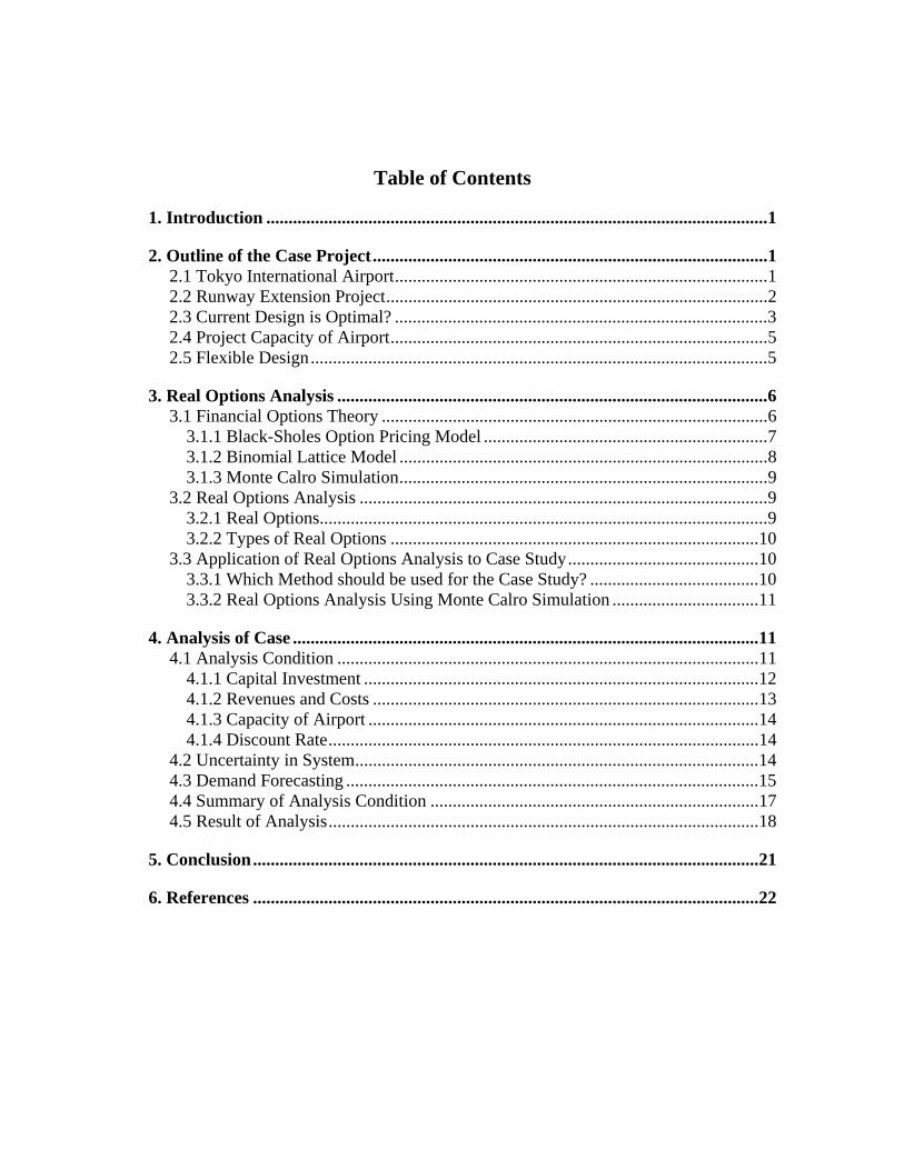
Table of Contents

1. Introduction .................................................................................................................1

2. Outline of the Case Project.........................................................................................1 2.1 Tokyo International Airport....................................................................................1 2.2 Runway Extension Project......................................................................................2 2.3 Current Design is Optimal? ....................................................................................3 2.4 Project Capacity of Airport.....................................................................................5 2.5 Flexible Design.......................................................................................................5

3. Real Options Analysis .................................................................................................6 3.1 Financial Options Theory .......................................................................................6

3.1.1 Black-Sholes Option Pricing Model ................................................................7 3.1.2 Binomial Lattice Model ...................................................................................8 3.1.3 Monte Calro Simulation...................................................................................9

3.2 Real Options Analysis ............................................................................................9 3.2.1 Real Options.....................................................................................................9 3.2.2 Types of Real Options ...................................................................................10

3.3 Application of Real Options Analysis to Case Study...........................................10 3.3.1 Which Method should be used for the Case Study? ......................................10 3.3.2 Real Options Analysis Using Monte Calro Simulation .................................11

4. Analysis of Case .........................................................................................................11 4.1 Analysis Condition ...............................................................................................11

4.1.1 Capital Investment .........................................................................................12 4.1.2 Revenues and Costs .......................................................................................13 4.1.3 Capacity of Airport ........................................................................................14 4.1.4 Discount Rate.................................................................................................14

4.2 Uncertainty in System...........................................................................................14 4.3 Demand Forecasting .............................................................................................15 4.4 Summary of Analysis Condition ..........................................................................17 4.5 Result of Analysis.................................................................................................18

5. Conclusion..................................................................................................................21

6. References ..................................................................................................................22

12/14/2007 1.231 Planning and Design of Airport System Dai Ohama

1. Introduction

The Airport systems not only in the U.S. but also all over the world are now very

complex. However, all of them are not always designed optimally. Some facilities are

built excessively compared to their estimation during planning phases, others are required

improvement since they are too large for the actual situations. [1] For example, the size of

the New Denver Airport is too big, and as a matter of fact there is an unnecessary passenger

building. The Newark airport is unsuited for the actual transfer and international traffic,

and major changes should be required. The reason for them is that the master plan of these

airport systems did not anticipate future risks and uncertainties of possible changes in market

conditions, and did not consider the countermeasure of those real risks. Eventually, it leads

to losses or extra costs, and even losses of opportunities happen. Thus, the master plan is

often inflexible and inherently cannot respond to the risks. In order to respond to this

situation, it is essential to plan strategically by considering future risks and uncertainties and

by applying flexibility into design.

This project is to consider one of the possible effective ways to incorporate flexibility

into design by using real options analysis. The goal of this project is to demonstrate how

the flexible design is conducted and how it works. The case of “Tokyo International

Airport New Runway Extension Project” is applied as a case study.

2. Outline of the Case Project

2.1 Tokyo International Airport

Tokyo International Airport or Haneda Airport (HND) is located in the bay area, near

the center of Tokyo. Haneda Airport is the busiest and an important hub airport in Japan

for domestic air traffic.[2] Haneda Airport is consistently ranked among the world's busiest

passenger airports in terms of the number of passengers, and its ranking was fourth in 2006.

Currently it has three runways (Runway A: 3,500m, Runway B: 2,500m, Runway C:

3,000m), serving nearly 60 million passengers every year. The total capacity of Haneda

Airport is 296,000 aircraft (a/c) per year.

Term Project: Flexible Design of Airport System Page 1 of 22


Japan

Kyoto Tokyo

Chiba

Haneda Airport Yokohama

Tokyo

Tokyo Bay Osaka

Figure 2-1 Location

Figure 2-2 Tokyo Int’l Airport Source: Ministry of Land, Infrastructure and Transport in Japan, Kanto

Regional Development Bureau [2]

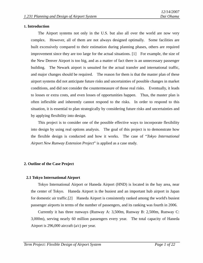
2.2 Runway Extension Project

However, its capacity has already reached a limit of airport capacity against the

increasing demand, and it is necessary to respond to the demand as soon as possible. In

order to solve this problem, Tokyo International Airport Extension Project was launched in

2002 to build 4th runway, which is called Runway D, to increase the total capacity of the

airport. [2] This extension enables the airport to have the capacity from of 296,000 a/c per

year to 407,000 a/c per year.

Extension Project “Runway D”

(Under Construction)

Runway A

Runway B

Runway C

Figure 2-3 Plan of New Runway Island in Haneda Airport Source: Ministry of Land, Infrastructure and Transport in Japan, Kanto Regional Development Bureau [2]



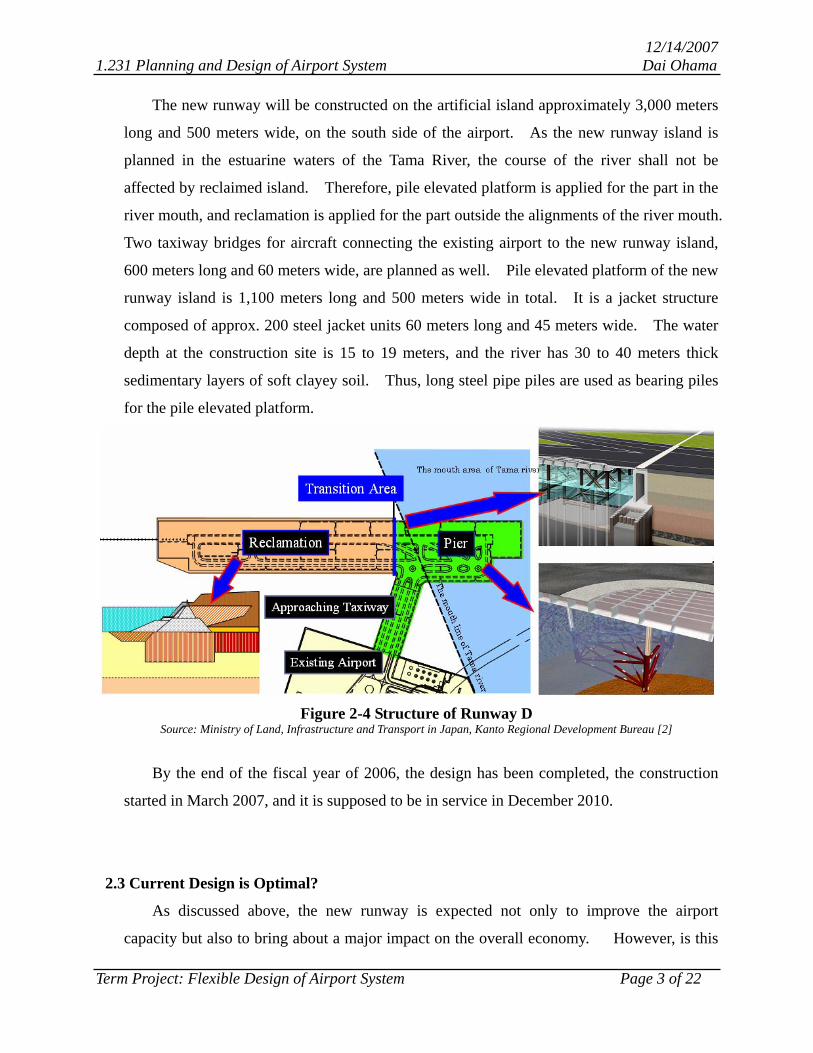
The new runway will be constructed on the artificial island approximately 3,000 meters

long and 500 meters wide, on the south side of the airport. As the new runway island is

planned in the estuarine waters of the Tama River, the course of the river shall not be

affected by reclaimed island. Therefore, pile elevated platform is applied for the part in the

river mouth, and reclamation is applied for the part outside the alignments of the river mouth.

Two taxiway bridges for aircraft connecting the existing airport to the new runway island,

600 meters long and 60 meters wide, are planned as well. Pile elevated platform of the new

runway island is 1,100 meters long and 500 meters wide in total. It is a jacket structure

composed of approx. 200 steel jacket units 60 meters long and 45 meters wide. The water

depth at the construction site is 15 to 19 meters, and the river has 30 to 40 meters thick

sedimentary layers of soft clayey soil. Thus, long steel pipe piles are used as bearing piles

for the pile elevated platform.

Figure 2-4 Structure of Runway D

Source: Ministry of Land, Infrastructure and Transport in Japan, Kanto Regional Development Bureau [2]

By the end of the fiscal year of 2006, the design has been completed, the construction

started in March 2007, and it is supposed to be in service in December 2010.

2.3 Current Design is Optimal?

As discussed above, the new runway is expected not only to improve the airport

capacity but also to bring about a major impact on the overall economy. However, is this



new project really optimal? Can the design of this project respond to the future

uncertainty?

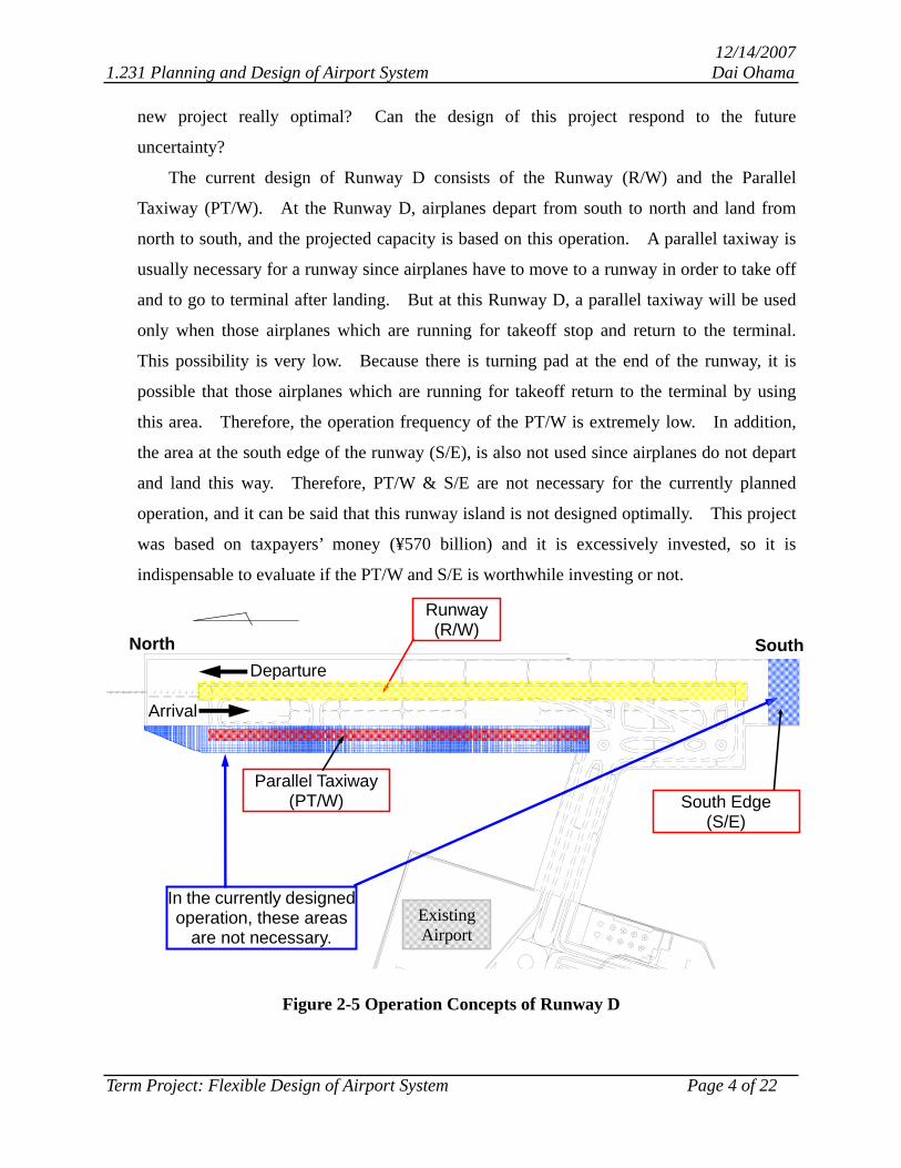
The current design of Runway D consists of the Runway (R/W) and the Parallel

Taxiway (PT/W). At the Runway D, airplanes depart from south to north and land from

north to south, and the projected capacity is based on this operation. A parallel taxiway is

usually necessary for a runway since airplanes have to move to a runway in order to take off

and to go to terminal after landing. But at this Runway D, a parallel taxiway will be used

only when those airplanes which are running for takeoff stop and return to the terminal.

This possibility is very low. Because there is turning pad at the end of the runway, it is

possible that those airplanes which are running for takeoff return to the terminal by using

this area. Therefore, the operation frequency of the PT/W is extremely low. In addition,

the area at the south edge of the runway (S/E), is also not used since airplanes do not depart

and land this way. Therefore, PT/W & S/E are not necessary for the currently planned

operation, and it can be said that this runway island is not designed optimally. This project

was based on taxpayers’ money (¥570 billion) and it is excessively invested, so it is

indispensable to evaluate if the PT/W and S/E is worthwhile investing or not.

Existing Airport

Runway (R/W)

Parallel Taxiway (PT/W)

In the currently designedoperation, these areas

are not necessary.

Departure

Arrival

North South

South Edge (S/E)

Figure 2-5 Operation Concepts of Runway D



These areas such as PT/W and S/E would be used if airplanes depart from north to south

and land from south to north. Thus, if they need this operation in the future, they should be

constructed, otherwise they should not be constructed.

2.4 Projected Capacity of Airport

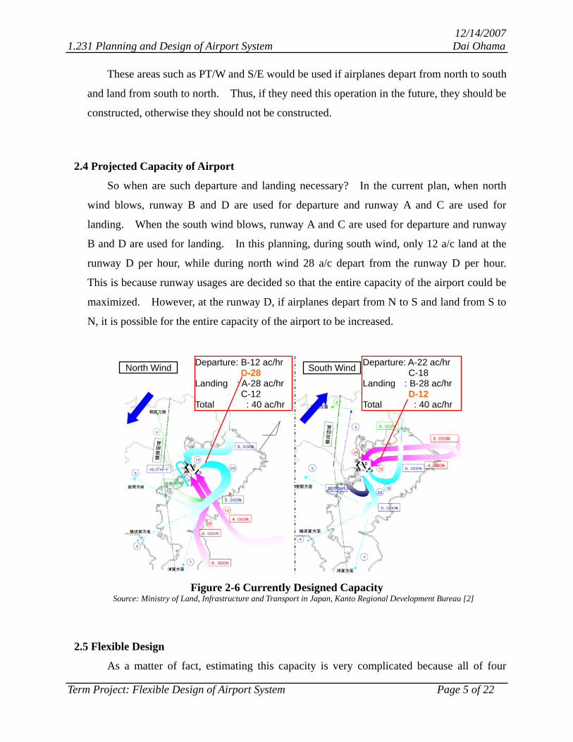
So when are such departure and landing necessary? In the current plan, when north

wind blows, runway B and D are used for departure and runway A and C are used for

landing. When the south wind blows, runway A and C are used for departure and runway

B and D are used for landing. In this planning, during south wind, only 12 a/c land at the

runway D per hour, while during north wind 28 a/c depart from the runway D per hour.

This is because runway usages are decided so that the entire capacity of the airport could be

maximized. However, at the runway D, if airplanes depart from N to S and land from S to

N, it is possible for the entire capacity of the airport to be increased.

North Wind South Wind Departure: B-12 ac/hr D-28 Landing : A-28 ac/hr C-12 Total : 40 ac/hr

Departure: A-22 ac/hr C-18 Landing : B-28 ac/hr D-12 Total : 40 ac/hr

Figure 2-6 Currently Designed Capacity Source: Ministry of Land, Infrastructure and Transport in Japan, Kanto Regional Development Bureau [2]

2.5 Flexible Design

As a matter of fact, estimating this capacity is very complicated because all of four



runways’ capacities are related complexly to one another. So, in this project, estimating

this capacity is outside of the scope of the goal. I assume that the opposite departure (from

north to south) and landing (from south to north) could increase the total capacity of the

airport. In other words, PT/W and S/E could increase the capacity. If the demand is more

than the capacity, PT/W and S/E should be constructed. If the demand is less than the

capacity, it’s not necessary to construct them. Therefore, PT/W and R/E should be

constructed when they become necessary. In other words, they don’t have to be

constructed until the demand of passengers exceeds the projected capacity. If such

flexibility is incorporated into design, managers are able to respond to future risks and

uncertainties such as demand of passengers. Therefore, flexible design can minimize the

initial investment, reduce risks, respond to uncertainties, and maximize the value of the

project. By doing so, this runway extension project would be optimized.

3. Real Options Analysis

In order to evaluate those projects, one of the best possible ways is real options analysis,

which is an evaluation method for those projects which involve decision opportunities.

Real options analysis is the application of financial options theory to the actual projects such

as infrastructure developments, real asset investments, research and development, and so on.

In these projects, those who make decision generally have options such as the option to defer,

the option to defer, and the option to abandon. In this case study, the option to expand

should be applied.

3.1 Financial Options Theory

Financial options theory is a basis for the real options analysis. In finance, an option

contract is an agreement where the owner has the right, but not the obligation, to buy or sell

an “underlying asset,” such as a stock, at a pre-determined price on or before the expiration

date. [3]

There are two types of options in terms of the right. A call option refers to the right to

buy a stock at the strike price, the pre-determined price. A put option refers to the right to

sell a stock at the strike price. [3] Options are also divided into two categories in terms of



expiration date. An American option is exercised when the owners are allowed to exercise

them on or before the expiration date. A European option is exercised only on the

expiration date. [3]

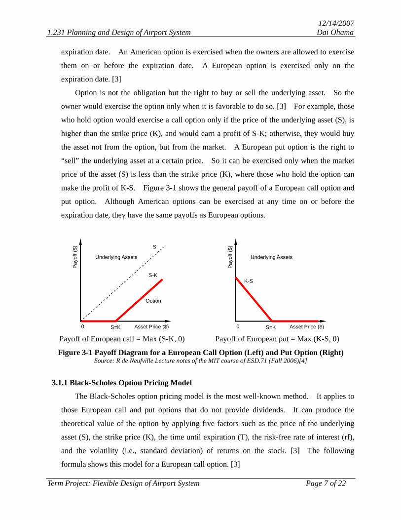
Option is not the obligation but the right to buy or sell the underlying asset. So the

owner would exercise the option only when it is favorable to do so. [3] For example, those

who hold option would exercise a call option only if the price of the underlying asset (S), is

higher than the strike price (K), and would earn a profit of S-K; otherwise, they would buy

the asset not from the option, but from the market. A European put option is the right to

“sell” the underlying asset at a certain price. So it can be exercised only when the market

price of the asset (S) is less than the strike price (K), where those who hold the option can

make the profit of K-S. Figure 3-1 shows the general payoff of a European call option and

put option. Although American options can be exercised at any time on or before the

expiration date, they have the same payoffs as European options.

Asset Price ($)

Pay

off (

$)

Underlying Assets

S

S-K

S=K0

Option

Payoff of European call = Max (S-K, 0)

Asset Price ($)

Pay

off (

$)

Underlying Assets

K-S

S=K0 Payoff of European put = Max (K-S, 0)

Figure 3-1 Payoff Diagram for a European Call Option (Left) and Put Option (Right) Source: R de Neufville Lecture notes of the MIT course of ESD.71 (Fall 2006)[4]

3.1.1 Black-Scholes Option Pricing Model

The Black-Scholes option pricing model is the most well-known method. It applies to

those European call and put options that do not provide dividends. It can produce the

theoretical value of the option by applying five factors such as the price of the underlying

asset (S), the strike price (K), the time until expiration (T), the risk-free rate of interest (rf),

and the volatility (i.e., standard deviation) of returns on the stock. [3] The following

formula shows this model for a European call option. [3]



( ) ( )21 dNeKdNSC Trf ⋅⋅−⋅= −

Where C: Theoretical value of a European call option with no dividends

( ) ( )T

TrKSd f

σ

σ ⋅++=

2//ln 2

1

Tdd σ−= 12

N(x): Cumulative probability function for a standardized normal distribution

The following formula shows the theoretical value of European put options.

( ) ( )12 dNSdNeKP Trf −⋅−−⋅⋅= −

Where P: Theoretical value of a European put option with no dividends

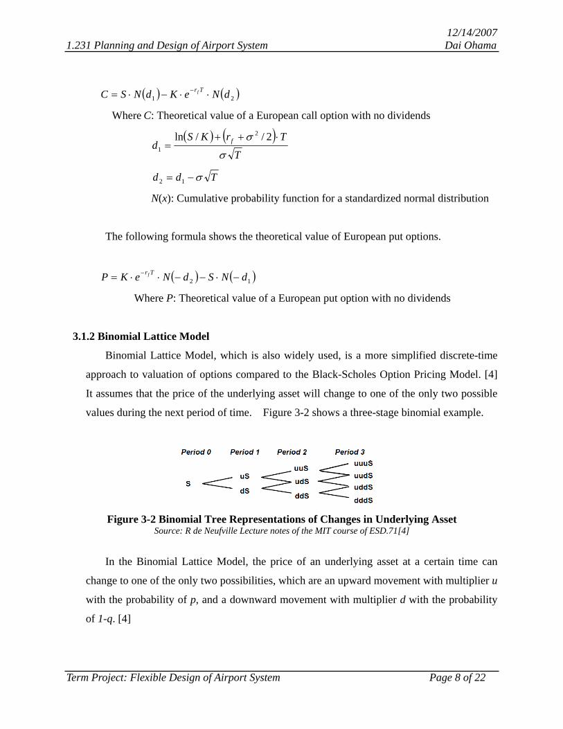
3.1.2 Binomial Lattice Model

Binomial Lattice Model, which is also widely used, is a more simplified discrete-time

approach to valuation of options compared to the Black-Scholes Option Pricing Model. [4]

It assumes that the price of the underlying asset will change to one of the only two possible

values during the next period of time. Figure 3-2 shows a three-stage binomial example.

Figure 3-2 Binomial Tree Representations of Changes in Underlying Asset

Source: R de Neufville Lecture notes of the MIT course of ESD.71[4]

In the Binomial Lattice Model, the price of an underlying asset at a certain time can

change to one of the only two possibilities, which are an upward movement with multiplier u

with the probability of p, and a downward movement with multiplier d with the probability

of 1-q. [4]



( ) Tdvp

ued

euT

T

Δ+=

==

=Δ−

Δ

/5.05.0

/1σ

σ

3.1.3 Monte Calro Simulation

Monte Calro Simulation is an analytical method that generates the stochastic

distribution of possible outcome that correspond to probability-distributed sampled inputs.

[5] Because of the development of computer technology, large computer simulation such

as Monte Calro Simulation can be constructed easily. Spread sheet software such as

Microsoft Excel is the tool for conducting Monte Calro Simulation.

3.2 Real Options Analysis

In the previous section, financial options theory including Black-Scholes option pricing

model, Binomial Lattice Model, and Monte Calro Simulation were introduced. In this

section, real options analysis, which was the application of financial options theory to the

actual projects, is introduced.

3.2.1 Real Options

Real option is the option to undertake some business decision under high uncertainty.

In real options analysis, they are associated with flexibilities in designing systems or the

evolution of projects. [4] Option - like flexibilities are included in systems and projects,

represent opportunities to increase the value of the project through design or through

management actions. [4] It is not obligation, and only when future asset price is preferable

for you, you can exercise it, otherwise you don’t have to do it. This allows

decision-makers to avoid downside losses as well as to obtain upside opportunities. These

flexibilities are called “real” options. [4] Managers have applied real options analysis to

business strategies including large-scale engineering systems. Although real options are

very similar to financial options, they are different from financial options in terms of what

should be assessed and the time span. [4] In financial options, the actual price such as



stock price is evaluated, while in real options, the value of the project itself is evaluated.

Financial options are usually very short span such as two years, while the time span of real

options is very long-term.

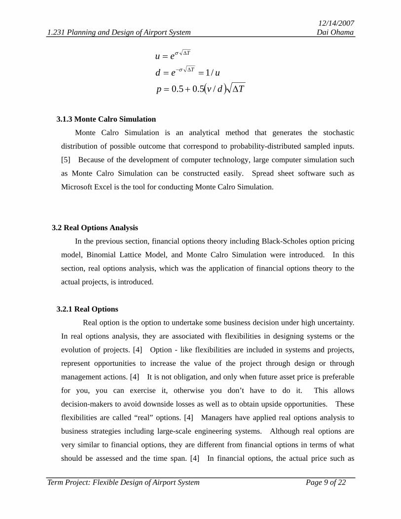
3.2.2 Types of Real Options

There are several types of real options, such as deferral options, abandonment options,

expansion options, growth options, and compound options. [6] Applying appropriate type

of options enables managers to actively manage risks and uncertainties. For example, in

this case study, expansion options is appropriate to be applied. In the current design, which

is inflexible design, the whole facilities such as a runway, a parallel taxiway, and a south

edge would be constructed at the initial construction. On the other hand, in flexible design

that should be proposed in this study, only a runway would be constructed at the initial

construction and then sometime after 10 years of operation, if the demand of passengers

exceeds the capacity, a parallel taxiway and a south edge should be constructed; otherwise

they would not be constructed. Thus, if uncertain demand is unfavorable, it is not

necessary to exercise the option. It is possible to reduce upfront capital investment and

therefore reduce losses. The Flexibility to expand them takes advantage of demand that is

higher than expected in the deterministic projections.

Value of Project

Payoff Expansion

No Expansion

Figure 3-3 Payoff of Expansion Option

3.3 Application of Real Options Analysis to Case Study

3.3.1 Which Method should be used for the Case Study



As introduced in section 3.1, there are three types of evaluation method in financial

options, and these are also applied to real options analysis. Black-Scholes option pricing

model and Binomial Lattice Model are widely used in financial options, but because they are

very complex and needs financial skills, they are not so widely used in real options in

engineering practice as in financial field. [7] Even if those methods are used appropriately,

it is very difficult to explain to those managers who are not familiar with financial skills. [7]

On the other hand, Monte Calro Simulation can be used more easily by using spread sheet

than those two methods. Compared to conventional methods using financial mathematics,

real options analysis using Monte Calro Simulation has advantages such as user friendly

procedure, being based on data availability in practice, and being easy to explain graphically.

[7] Thus real options analysis based on Monte Calro Simulation can be the appropriate as a

tool for the valuation method for this case study.

3.3.2 Real Options Analysis Using Monte Calro Simulation

In this case study, real options analysis using Monte Calro Simulation method is used

and its procedure is: 1) to estimate cash flows pro forma including capital investment, future

costs and revenues of the project, and calculate the economic value of currently designed

case, 2) to explore the effects of uncertainty by simulating possible scenarios, each of which

leads to a various NPVs, and the collection of each scenario generate both an “expected net

present value” (ENPV) and the distribution of possible outcomes for a project by

demonstrating cumulative distribution functions, and 3) to explore ways to avoid the

downside risk and take advantage of upside potential by exercising options. [7]

4. Analysis of Case - Tokyo Int’l Airport New Runway Extension Project

4.1 Analysis Condition

In order to conduct real options analysis, it is necessary to set up analysis conditions

such as cash flow pro forma including capital investment, revenue scheme, operating and

maintenance costs.

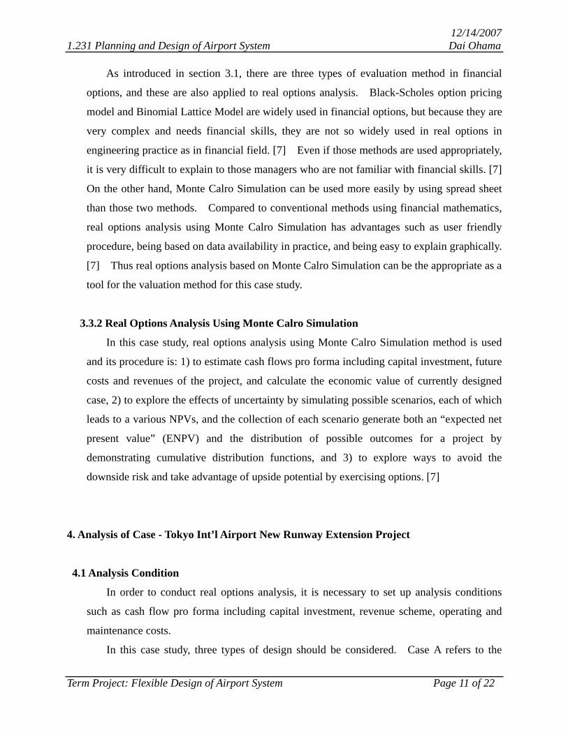
In this case study, three types of design should be considered. Case A refers to the



current design that government actually planned and that would construct the whole runway

island, including a parallel taxiway and a south edge. This design does not include

flexibility.

Case B refers to the design that constructs the whole runway island in the same way as

Case A. But this design recognizes future uncertainty which is demand of passengers,

while Case A considers deterministic projection of the demand of passengers.

Case C refers to the design that constructs only runway area without parallel taxiway

and south edge of the runway at the initial construction, and expands the parallel taxiway

and south edge after 10 years operation if the demand exceeds the capacity of the airport for

two consecutive years.

Table 4-1 shows the summary of case of analysis.

Table 4-1 Cases of Analysis

Case Initial Investment

Future Uncertainty Flexibility

Case A R/W, PT/W & SE N/A N/A

Case B R/W, PT/W & SE Recognizing N/A

Case C R/W Recognizing Future Expansion PT/W & SE

Source: Applied R de Neufville,et al [7]

4.1.1 Capital Investment

Capital investment here means the initial construction fee and the expansion fee of the

parallel taxiway and the south edge. In the “New Runway Extension Project”, the

construction fee is ¥570 billion, [2] so the initial investment in Case A and Case B is ¥570

billion. In Case C, I assume that the initial investment can be set by prorating the area

where it needs. In the area of the taxiway (827,625m2), the structure of the runway island

is landfill (¥64,700/m2), [2] so the construction fee is ¥53.55 billion. In the area of the

south edge (45,120m2), the structure of the runway island is piled pier (¥786,500/m2), [2] so

the construction fee is ¥35.48 billion. Therefore, considering the bank revetment area

(assumed 5% extra) and the joint area for the both areas so that the expansion could be

possible, the initial construction fee of Case C is ¥505 billion. ([570-(53.55+35.48)]*1.05)



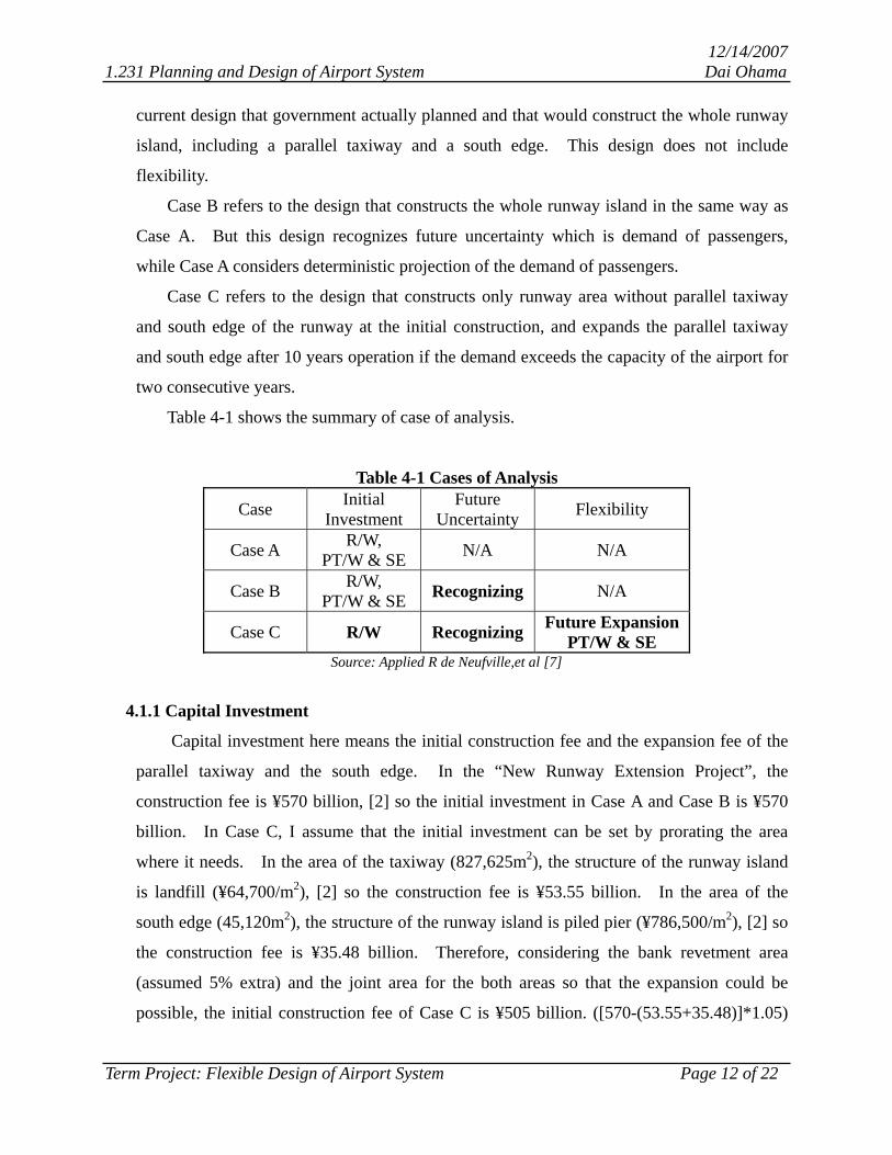
The expansion cost of Case C is only the area of taxiway and the south edge, which is the

same as the difference between the initial cost of Case A, B and that of Case C.

Considering the extra fee of the joint area (assumed 10% extra), the expansion fee is ¥97.9

billion. ((53.55+35.48)*1.05) The initial investment is assumed to be paid equally every

year through the construction for 4 years, while the expansion investment is supposed to be

paid equally every year for 2 years.

Runway (R/W)

Parallel Taxiway (Landfill)

827,625m2

South Edge (Piled Pier) 45,120m2

Figure 4-1 Expansion Area of Runway D

4.1.2 Revenues and Costs

There are several types of revenues and costs in the airport system such as from

aeronautical charges, non-aeronautical charges, and off-airport or non-operate charges. [8]

In the current operation of Tokyo Int’l Airport, these charges applies, but in terms of a

runway, aeronautical charges, which is the charges for services or facilities directly related to

the processing of aircraft and their passengers, is the main charge. [8] The aeronautical

charges have several categories such as landing charge, terminal-area air navigation charge,

passenger service charge in terminals, security charge, charges for airport noise, and so on.

[8] In terms of a runway, landing charge is the main source of the revenue. Thus, I

assume that the revenue is only from the landing charge. The current landing charge in

Tokyo Int’l Airport as of 2006 is ¥490,000 for B747-400D, ¥350,000 for B777-200, and

¥230,000 for B777-724, and so on. [9] I set the average landing fee of this airport as

¥332,000 / aircraft by assuming the probabilities for each type of aircraft of 23% for

B747-400D, 35% for B777-200D, and 41% for B767-300. I also assume that this landing

charge is fixed for the next 20 years. For the simplicity, I also set the revenue for each year

is landing charge multiplied by the minimum of the number of passenger or the capacity.



Costs for the operation and maintenance are categorized into the ones above. From the

past disclosed information by the government, operating and maintenance cost in all airports

in Japan in 2005 was ¥147.4 billion. [10] I assume that these costs depend on the scale of

air traffic. The whole air traffic in Japan in 2005 was 1,431,000 and 300,000 in Tokyo Int’l

Airport, which is about 20% of the whole traffic, so the operating and maintenance costs for

Tokyo Int’l Airport in each year is assumed ¥29.48 billion, which is also assumed equally for

the current three runways. So the operating cost and maintenance costs for the one runway

is one-third of ¥29.48, which is equal to ¥9.84 billion. In addition, in the current

construction plan indicates that the specific maintenance cost for the runway D is ¥100

billion for the next 30 years. Thus the maintenance cost of ¥3.33 billion should also be

included in the operating and maintenance cost for the new runway. Therefore, the

operating and maintenance costs for the runway D are set as ¥13.17 billion.

4.1.3 Capacity of Airport

According to the Ministry of Land, Infrastructure and Transport in Japan, the improved

maximum capacity of the airport by the runway extension in Tokyo Int’l Airport is 40

aircrafts per hour, and it estimated this capacity can accommodate 87 million passengers per

year. [2] So the capacity in terms of the number of passenger in this airport is 87 million.

4.1.4 Discount Rate

Discount rate is the opportunity cost of capital, and it can be calculated by the capital

asset pricing model (CAPM). CAPM requires the risk-free rate of interest, the sensitivity

of specific project or company to stock price, and the expected rate of return of the market.

However, the government used the discount rate of 4% when it assessed not only this project

but also any airport related project. [11] Thus, the discount rate of 4% is also used in this

case study.

4.2 Uncertainty in System

There are usually a lot of uncertainties in large-scale engineering systems which include

technical change, economic change, regulatory change, industrial change, political change,

and so on. [4] This case also includes a lot of uncertainties such as demand of the number



of passengers, capital investment in the future, the operating and maintenance costs, and

unexpected events in the future. For the sake of the simplicity, I set only demand of the

number of passengers as uncertainty. When forecasting the number of passenger in airports,

the time span should be considered at most 20 years span and the volatility, which is the

range of the chance the demand is higher or lower, should be considered by plus or minus

50%. [12]

4.3 Demand Forecasting

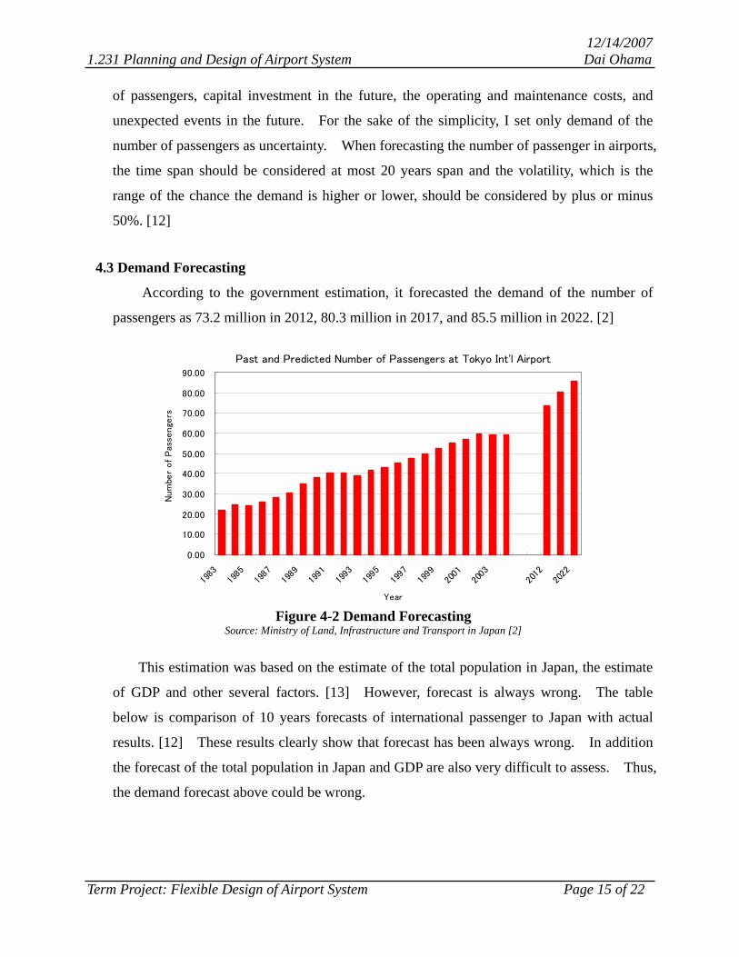
According to the government estimation, it forecasted the demand of the number of

passengers as 73.2 million in 2012, 80.3 million in 2017, and 85.5 million in 2022. [2]

Past and Predicted Number of Passengers at Tokyo Int'l Airport

0.00

10.00

20.00

30.00

40.00

50.00

60.00

70.00

80.00

90.00

1983

1985

1987

1989

1991

1993

1995

1997

1999

2001

2003

2012

2022

Year

Num

ber

of

Pas

senge

rs

Figure 4-2 Demand Forecasting

Source: Ministry of Land, Infrastructure and Transport in Japan [2]

This estimation was based on the estimate of the total population in Japan, the estimate

of GDP and other several factors. [13] However, forecast is always wrong. The table

below is comparison of 10 years forecasts of international passenger to Japan with actual

results. [12] These results clearly show that forecast has been always wrong. In addition

the forecast of the total population in Japan and GDP are also very difficult to assess. Thus,

the demand forecast above could be wrong.



Table 4-2 Comparison of 10-year forecasts of international passengers to Japan with actual results

Forecast Passengers (millions) Percent error For Done in Actual Forecast Over actual

1980 1970 12.1 20.0 65 1985 1975 17.6 27.0 53 1990 1980 31.0 39.5 27 1995 1985 43.6 37.9 (13)

Source: R. de Neufville, A. Odoni, Airport Systems: Planning, Design, and Management[12]

However, when assessing the real options analysis, it is necessary to rely on some

forecasts, although they are nothing but estimation. Thus, in this case study, the demand

curve that is based on the estimation of the total population and the estimation of GDP in

Japan should be considered. The important thing is to recognize that this forecast is just an

assumption and to evaluate this by using various demand scenarios with volatility.

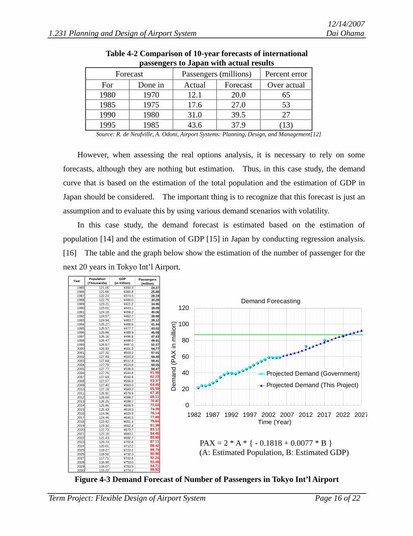
In this case study, the demand forecast is estimated based on the estimation of

population [14] and the estimation of GDP [15] in Japan by conducting regression analysis.

[16] The table and the graph below show the estimation of the number of passenger for the

next 20 years in Tokyo Int’l Airport. Year Population

(Thousands)GDP

(in trillion)Passengers

(million)1985 121.05 ¥350.3 24.271986 121.66 ¥360.8 25.881987 122.24 ¥374.5 28.191988 122.75 ¥400.0 30.281989 123.21 ¥421.2 34.961990 123.61 ¥443.1 38.091991 124.10 ¥458.2 40.061992 124.57 ¥462.7 39.981993 124.94 ¥463.7 39.121994 125.27 ¥468.8 41.441995 125.57 ¥477.7 43.021996 125.86 ¥489.9 45.081997 126.16 ¥496.8 47.431998 126.47 ¥488.0 49.911999 126.67 ¥487.0 52.272000 126.93 ¥501.3 54.772001 127.32 ¥503.2 57.012002 127.49 ¥503.9 59.492003 127.69 ¥512.8 59.412004 127.79 ¥524.6 59.052005 127.77 ¥538.9 59.472006 127.76 ¥544.8 61.08

62.2363.3764.4965.5967.3569.1170.8772.6374.3976.1477.8979.6481.3883.1284.4685.8087.1188.4289.7090.9892.2493.4894.71

2007 127.69 ¥550.82008 127.57 ¥556.92009 127.40 ¥563.02010 127.18 ¥569.22011 126.91 ¥578.92012 126.60 ¥588.72013 126.25 ¥598.72014 125.86 ¥608.92015 125.43 ¥619.32016 124.96 ¥629.82017 124.46 ¥640.52018 123.92 ¥651.42019 123.34 ¥662.42020 122.73 ¥673.72021 122.10 ¥683.12022 121.43 ¥692.72023 120.74 ¥702.42024 120.01 ¥712.22025 119.27 ¥722.22026 118.50 ¥732.32027 117.71 ¥742.62028 116.90 ¥753.02029 116.07 ¥763.52030 115.22 ¥774.2 95.92

Demand Forecasting

0

20

40

60

80

100

120

1982 1987 1992 1997 2002 2007 2012 2017 2022 2027Time (Year)

Dem

and

(PA

X in

mill

ion)

Projected Demand (Government)

Projected Demand (This Project)

PAX = 2 * A * { - 0.1818 + 0.0077 * B }

(A: Estimated Population, B: Estimated GDP)

Figure 4-3 Demand Forecast of Number of Passengers in Tokyo Int’l Airport



The demand curve shown in Figure 4-3 is still deterministic projection, and this is

usually used for the static analysis. However, it is essential to recognize and consider the

uncertainty in this demand forecasting. Thus, uncertainty is recognized in the model by

simulating possible scenarios. It indicates how fluctuations can be incorporated around

deterministic projections based on the relevant probability distribution. [17] In this case

study, 2,000 Monte Calro Simulations are generated where all of those simulations create

each demand scenarios over the 20 years span. Figure 4-4 shows some of the examples of

simulations of the uncertain demand. All of these scenarios can be considered and

incorporated into the calculation of the expected value of the plans statistically.

Demand Forecasting

0

20

40

60

80

100

120

1982 1987 1992 1997 2002 2007 2012 2017 2022 2027Time (Year)

Dem

and

(PAX

in m

illio

n)

Projected Demand (Government)Projected Demand (This Project)Demand scenario

Demand Forecasting

0

20

40

60

80

100

120

1982 1987 1992 1997 2002 2007 2012 2017 2022 2027Time (Year)

Dem

and

(PA

X in

mill

ion)


Demand Forecasting

0

20

40

60

80

100

120

1982 1987 1992 1997 2002 2007 2012 2017 2022 2027Time (Year)

Dem

and

(PA

X in

milli

on)


Demand Forecasting

0

20

40

60

80

100

120

1982 1987 1992 1997 2002 2007 2012 2017 2022 2027Time (Year)

Dem

and

(PA

X in

milli

on)


Figure 4-4 Examples of Simulation of the Uncertain Demand

4.4 Summary of Analysis Condition

The Table 4-3 shows the summary of analysis condition.



Table 4-3 Summary of Analysis Condition

Initial Investment

Future Expansion Perspective Simulation Option

Design A R/W, PT/W & SE N/A Deterministic No No

Design B R/W, PT/W & SE N/A Recognizing

Uncertainty Yes No

Design C R/W PT/W & SE Incorporating Flexibility Yes Yes

Source: Applied R de Neufville, S. Scholtes, T. Wang [7]

4.5 Result of Analysis

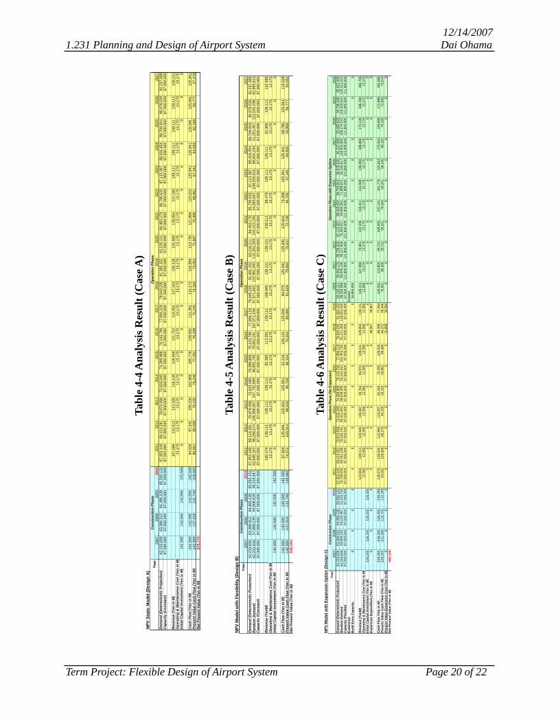
Table 4-4, 4-5, 4-6 shows the cash flow pro forma for three cases. Table 4-4 shows the

cash flow pro forma and calculating the NPV of the project assuming the demand of the

number of passengers grows as projected. (Case A) In this case, the expected NPV

(ENPV) of the project is ¥678.8 billion. However, this value is not realistic since the actual

demand of the number of passengers can change from this deterministic value.

Table 4-5 shows the cash flow pro forma and calculating the NPV of the project

recognizing uncertainty. (Case B) In this case, Monte Calro Simulation is conducted and it

produces 2,000 possible demand scenarios. The ENPV of this case is ¥638.3 billion. But

this ENPV is just one of the 2,000 scenarios. This simulation can generate 2,000 ENPV in

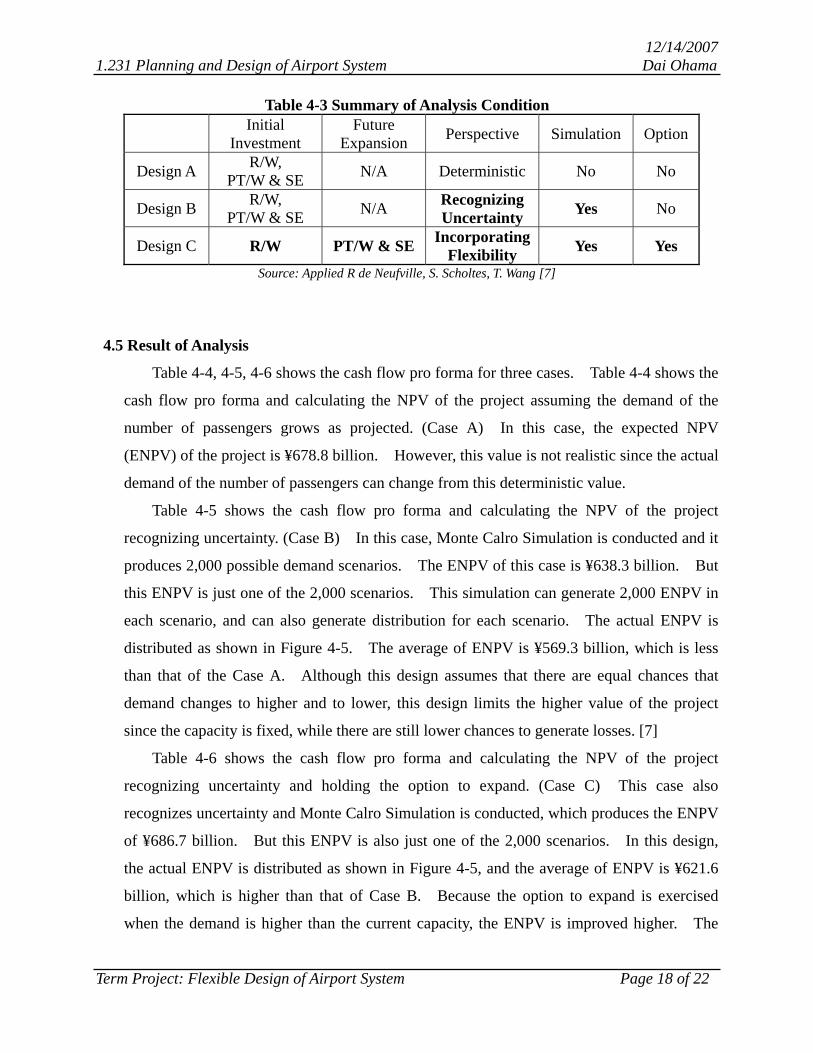
each scenario, and can also generate distribution for each scenario. The actual ENPV is

distributed as shown in Figure 4-5. The average of ENPV is ¥569.3 billion, which is less

than that of the Case A. Although this design assumes that there are equal chances that

demand changes to higher and to lower, this design limits the higher value of the project

since the capacity is fixed, while there are still lower chances to generate losses. [7]

Table 4-6 shows the cash flow pro forma and calculating the NPV of the project

recognizing uncertainty and holding the option to expand. (Case C) This case also

recognizes uncertainty and Monte Calro Simulation is conducted, which produces the ENPV

of ¥686.7 billion. But this ENPV is also just one of the 2,000 scenarios. In this design,

the actual ENPV is distributed as shown in Figure 4-5, and the average of ENPV is ¥621.6

billion, which is higher than that of Case B. Because the option to expand is exercised

when the demand is higher than the current capacity, the ENPV is improved higher. The



estimated value of the option exercised in order to incorporate the flexibility into design can

be calculated by the difference between the ENPV of Case C and that of Case B, which is

¥52.3 billion. Table 4-7 shows the summary of this analysis. Case C, which holds

flexibility in design has advantages over Case B in every aspect. Table 4-6 shows the

summary of the analysis. [7] The initial investment in Case C is less than that of Case B,

which means that the flexibility can reduce the initial investment. The ENPV, the

maximum and minimum NPV in Case C is higher than that of Case B, so the flexibility can

enhance the overall value of the project.

Cumulative distribution function

0.0%

10.0%

20.0%

30.0%

40.0%

50.0%

60.0%

70.0%

80.0%

90.0%

100.0%

200,000 300,000 400,000 500,000 600,000 700,000 800,000 900,000

Target value \ million

Prob

abili

ty

Case C Case B

Average ENPV(B)¥569.3 B

Average ENPV(C) ¥621.6 B

Option Value ¥52.3 B

Case A (¥678.7 B)

Figure 4-5 Cumulative Distribution Function (Value at Risk)

Table 4-7 Summary of the Analysis Case B

(No Flexibility)Case C

(with Flexibility) Initial Investment (¥ in billion) 570.0 505.0 ENPV (¥ in billion) 569.3 621.6 Minimum NPV (¥ in billion) 339.3 338.1 Maximum NPV (¥ in billion) 773.4 899.1




NPV

Mod

el w

ith E

xpan

sion

Opt

ion

(Des

ign

C)

2007

2008

2009

2010

2011

2012

2013

2014

2015

2016

2017

2018

2019

2020

2021

2022

2023

2024

2025

2026

2027

2028

2029

2030

Dem

and

(Det

erm

inis

tic P

roje

ctio

n)62

,233

,839

63,3

66,5

1264

,486

,139

65,5

9267

,353

,149

69,1

14,2

8170

,874

,568

72,6

33,3

4074

,389

,968

76,1

43,7

9077

,894

,119

79,6

40,2

3581

,381

,152

83,1

16,1

1184

,463

,179

85,7

95,6

3387

,113

,387

88,4

16,4

5489

,704

,914

90,9

78,5

3092

,237

,068

93,4

80,0

2994

,706

,438

95,9

15,4

30R

ando

m D

eman

d62

,233

,839

39,8

94,3

3554

,103

,487

51,5

25,7

0276

,708

,558

90,4

11,1

8678

,516

,141

85,4

21,8

4258

,639

,900

53,1

41,8

1310

1,46

3,79

281

,211

,366

116,

851,

429

99,5

58,9

9980

,045

,196

46,2

17,6

5876

,364

,557

94,0

04,5

8171

,889

,072

85,1

06,6

1711

8,00

2,96

010

8,27

4,52

311

6,42

3,51

413

4,21

1,22

1C

a

,131

paci

ty (F

lexi

ble)

87,0

00,0

0087

,000

,000

87,0

00,0

0087

,000

,000

87,0

00,0

0087

,000

,000

87,0

00,0

0087

,000

,000

87,0

00,0

0087

,000

,000

87,0

00,0

0087

,000

,000

87,0

00,0

0087

,000

,000

121,

800,

000

121,

800,

000

121,

800,

000

121,

800,

000

121,

800,

000

121,

800,

000

121,

800,

000

121,

800,

000

121,

800,

000

121,

800,

000

Expa

nsio

nE

x pan

dB

uild

Ext

ra C

apac

ity0

00

00

00

00

00

00

34,8

00,0

000

00

00

00

00

0

Rev

enue

(Yen

M)

122,

655

139,

111

125,

545

136,

587

93,7

6484

,972

139,

111

129,

855

139,

111

139,

111

127,

990

73,9

0112

2,10

515

0,31

111

4,94

913

6,08

318

8,68

317

3,12

818

6,15

819

4,75

5O

pera

ting

& M

aint

enan

ce C

ost (

Yen

in M

)12

,580

12,5

8012

,580

12,5

8012

,580

12,5

8012

,580

12,5

8012

,580

12,5

8013

,170

13,1

7013

,170

13,1

7013

,170

13,1

7013

,170

13,1

7013

,170

13,1

70In

itial

Cap

ital I

nves

tmen

t (Ye

n in

M)

126,

255

126,

255

126,

255

126,

255

00

00

00

00

00

00

00

00

00

00

Expa

nsio

n Ex

pend

iture

(Yen

in M

)0

00

00

00

00

00

48,9

6748

,967

00

00

00

00

00

0

Cas

h Fl

ow (Y

en in

M)

-126

,255

-126

,255

-126

,255

-126

,255

110,

075

126,

531

112,

965

124,

007

81,1

8472

,392

126,

531

68,3

0877

,564

126,

531

114,

820

60,7

3110

8,93

513

7,14

110

1,77

912

2,91

317

5,51

315

9,95

817

2,98

818

1,58

5Pr

esen

t Val

ue C

ash

Flow

(Yen

in M

)-1

26,2

55-1

21,3

99-1

16,7

29-1

12,2

4094

,092

103,

999

89,2

7894

,235

59,3

2050

,862

85,4

8044

,372

48,4

4675

,991

66,3

0633

,722

58,1

6170

,404

50,2

4158

,340

80,1

0270

,195

72,9

9373

,674

Pres

ent V

alue

Exp

ansi

on C

ost (

Yen

in M

)0

00

00

00

00

00

31,8

0830

,584

00

00

00

00

00

0N

et P

rese

nt V

alue

(Yen

in M

)68

6,72

8

Con

stru

ctio

n Ph

ase

Ope

ratio

n Ph

ase

with

Exp

ansi

on O

ptito

nO

peYe

arra

tion

Phas

e (N

o Ex

pans

ion)

NPV

Mod

el w

ith F

lexi

bilit

y (D

esig

n B

)

2007

2008

2009

2011

2012

2013

2014

2015

2016

2017

2018

2019

2020

2021

2022

2023

2024

2025

2026

2027

Dem

and

2010

(Det

erm

inis

tic P

roje

ctio

n)62

,233

,839

63,3

66,5

1264

,486

,139

65,5

9267

,353

,149

69,1

14,2

8170

,874

,568

72,6

33,3

4074

,389

,968

76,1

43,7

9077

,894

,119

79,6

40,2

3581

,381

,152

83,1

16,1

1184

,463

,179

85,7

95,6

3387

,113

,387

88,4

16,4

5489

,704

,914

90,9

78,5

3092

,237

,068

Ran

dom

Dem

and

62,1

31,2

33,8

3957

,868

,139

65,9

08,6

2938

,319

,447

62,6

49,1

5396

,258

,574

105,

906,

007

107,

792,

690

40,8

92,7

4570

,852

,191

107,

971,

158

67,5

71,6

0210

2,96

1,94

311

5,20

2,20

910

3,42

3,18

554

,083

,607

108,

556,

015

89,9

44,2

4451

,261

,467

122,

025,

498

82,9

89,8

13C

a pac

ity (C

onst

ant)

87,0

00,0

0087

,000

,000

87,0

00,0

0087

,000

,000

87,0

00,0

0087

,000

,000

87,0

00,0

0087

,000

,000

87,0

00,0

0087

,000

,000

87,0

00,0

0087

,000

,000

87,0

00,0

0087

,000

,000

87,0

00,0

0087

,000

,000

87,0

00,0

0087

,000

,000

87,0

00,0

0087

,000

,000

87,0

00,0

00

Rev

enue

(Yen

M)

100,

174

139,

111

139,

111

139,

111

65,3

8611

3,29

113

9,11

110

8,04

513

9,11

113

9,11

113

9,11

186

,478

139,

111

139,

111

81,9

6613

9,11

113

2,69

8O

pera

ting

& M

aint

enan

ce C

ost (

Yen

in M

)13

,170

13,1

7013

,170

13,1

7013

,170

13,1

7013

,170

13,1

7013

,170

13,1

7013

,170

13,1

7013

,170

13,1

7013

,170

13,1

7013

,170

Initi

al C

a pita

l Inv

estm

ent (

Yen

in M

)14

2,50

014

2,50

014

2,50

014

2,50

00

00

00

00

00

00

00

00

00

Cas

h Fl

ow (Y

en in

M)

-142

,500

-142

,500

-142

,500

-142

,500

87,0

0412

5,94

112

5,94

112

5,94

152

,216

100,

121

125,

941

94,8

7512

5,94

112

5,94

112

5,94

173

,308

125,

941

125,

941

68,7

9612

5,94

111

9,52

8Pr

esen

t Val

ue C

ash

Flow

(Yen

in M

)-1

42,5

00-1

37,0

19-1

31,7

49-1

26,6

8274

,372

103,

514

99,5

3395

,705

38,1

5470

,343

85,0

8161

,629

78,6

6275

,637

72,7

2840

,705

67,2

4164

,655

33,9

5959

,777

54,5

51N

et P

rese

nt V

alue

(Yen

in M

)63

8,29

4

Con

stru

ctio

n Ph

ase

Ope

ratio

n Ph

ase

Year

NPV

Sta

tic M

odel

(Des

ign

A)

2007

2008

2009

2011

2012

2013

2014

2015

2016

2017

2018

2019

2020

2021

2022

2023

2024

2025

2026

2027

Dem

and

2010

(Det

erm

inis

tic P

roje

ctio

n)62

,233

,839

63,3

66,5

1264

,486

,139

65,5

92,1

3167

,353

,149

69,1

14,2

8170

,874

,568

72,6

33,3

4074

,389

,968

76,1

43,7

9077

,894

,119

79,6

40,2

3581

,381

,152

83,1

16,1

1184

,463

,179

85,7

95,6

3387

,113

,387

88,4

16,4

5489

,704

,914

90,9

78,5

3092

,237

,068

Ca p

acity

(Con

stan

t)87

,000

,000

87,0

00,0

0087

,000

,000

87,0

00,0

0087

,000

,000

87,0

00,0

0087

,000

,000

87,0

00,0

0087

,000

,000

87,0

00,0

0087

,000

,000

87,0

00,0

0087

,000

,000

87,0

00,0

0087

,000

,000

87,0

00,0

0087

,000

,000

87,0

00,0

0087

,000

,000

87,0

00,0

0087

,000

,000

Rev

enue

(Yen

in M

)10

7,69

611

0,51

211

3,32

611

6,13

911

8,94

812

1,75

212

4,55

112

7,34

313

0,12

613

2,90

013

5,05

413

7,18

513

9,11

113

9,11

113

9,11

113

9,11

113

9,11

1O

pera

ting

& M

aint

enan

ce C

ost (

Yen

in M

)13

,170

13,1

7013

,170

13,1

7013

,170

13,1

7013

,170

13,1

7013

,170

13,1

7013

,170

13,1

7013

,170

13,1

7013

,170

13,1

7013

,170

Initi

al C

a pita

l Inv

estm

ent (

Yen

in M

)14

2,50

014

2,50

014

2,50

014

2,50

00

00

00

00

00

00

00

00

00

Cas

h Fl

ow (Y

en in

M)

-142

,500

-142

,500

-142

,500

-142

,500

94,5

2697

,342

100,

156

102,

969

105,

778

108,

582

111,

381

114,

173

116,

956

119,

730

121,

884

124,

015

125,

941

125,

941

125,

941

125,

941

125,

941

Pres

ent V

alue

Cas

h Fl

ow (Y

en in

M)

-142

,500

-137

,019

-131

,749

-126

,682

80,8

0180

,008

79,1

5578

,248

77,2

9176

,288

75,2

4574

,164

73,0

5171

,907

70,3

8568

,861

67,2

4164

,655

62,1

6859

,777

57,4

78N

et P

rese

nt V

alue

(Yen

in M

)67

8,77

0

Con

stru

ctio

n Ph

ase

Ope

ratio

n Ph

ase

Year

Tabl

e 4-

4 A

naly

sis R

esul

t (C

ase A

)

Tabl

e 4-

5 A

naly

sis R

esul

t (C

ase

B)

Tabl

e 4-

6 A

naly

sis R

esul

t (C

ase

C)


5. Conclusion

There are a lot of facilities that are not designed optimally in airport systems. The

master plan of those designs does not anticipate and consider future risks and uncertainties.

Thus, inflexible design cannot manage risks and uncertainties, and it leads to losses. In

order to solve this problem, it is essential to incorporate flexibility into design. As

demonstrated in the case study in this paper, the real option analysis is the useful way to

recognize uncertainty and incorporate flexibility into design. The case study demonstrated

that flexibility can enhance the expected value of the project, and reduce the possible losses

by using the option to expand. Also it can demonstrate that flexibility can keep the initial

cost lower than that of the current design. Therefore, at the initial construction phase, only

runway should be constructed and if the demand of the number of passenger exceeds the

capacity after 10 years operation, a parallel taxiway and a south edge should be constructed.

Furthermore, real options analysis using Monte Calro Simulation is very useful in that it just

focuses on the ENPV of options and it does not require any financial skills unlike typical

financial options approaches such as Black-Sholes option pricing model and binomial lattice

model. Thus, those who are in charge of design can relatively easily use this method.

Flexible design thus enables projects to be optimized and reduce excessiveness and losses in

airport systems.



6. Reference

[1] R. de Neufville, Lecture note of the MIT course of 1.231: Planning and Design of Airport System (Fall 2007).

[2] Ministry of Land, Infrastructure and Transport in Japan, Outline of Tokyo Int’l Airport New Runway Extension Project, 2007. http://www.mlit.go.jp/koku/04_outline/01_kuko/02_haneda/index.html

[3] R. A. Brealey, S.C. Myers, and F. Allen, Principles of Corporate Finance, 8th ed., (New York: McGraw-Hill Publishing Company, 2005).

[4] R. de Neufville, Lecture notes of the MIT course of ESD.71: Engineering Systems Analysis for Design (Fall 2006).

[5] K. Hodota, “R&D and Deployment Valuation of Intelligent Transportation Systems: A Case Example of the Intersection Collision Avoidance Systems,” M.S. Thesis in Master of Science in Transportation, MIT, Cambridge, MA, 2006.

[6] T. Copeland, T. Koller, J. Murrin, Valuation: Measuring and Managing the Value of Companies, Fourth Edition (McKinsey & Company Inc., 2002).

[7] R. de Neufville, S. Scholtes, T. Wang, Valuing Real Options by Spread Sheet : Parking Garage Case Example, January 2005.

[8] A. Odoni, Lecture notes of the MIT course of 1.231: Planning and Design of Airport System (Fall 2007).

[9] Ministry of Land, Infrastructure and Transport in Japan, Civil Aviation Breau. http://www.mlit.go.jp/singikai/koutusin/koku/seibi/14/images/shiryou1_22.pdf

[10] Ministry of Land, Infrastructure and Transport in Japan, Survey of the Air Traffic Condition in Japan, 2003, http://www.mlit.go.jp/kisha/kisha03/12/120523_3/05.pdf

[11] Katsuya Hihara, Research for New Operation System of Transportation Policy Considering Uncertainty, 2004, Policy Research Institute for Land Infrastructure and Transport, https://www.mlit.go.jp/pri/houkoku/gaiyou/pdf/kkk9.pdf

[12] R. de Neufville, A. Odoni, Airport Systems: Planning, Design, and Management, 2nd ed., (New York: McGraw-Hill Publishing Company, 2003)

[13] Ministry of Land, Infrastructure and Transport in Japan, Forecast of air traffic, http://www.mlit.go.jp/singikai/koutusin/koku/07_9/01.pdf

[14] National Institute of Population and Social Security Research, Forecast of Population http://www.ipss.go.jp/syoushika/tohkei/suikei07/suikei.html#chapt1-1

[15] Ministry of Land, Infrastructure and Transport in Japan, Transition and Forecast of GDP, http://www.mlit.go.jp/road/kanren/suikei/7-1.pdf

[16] R. de Neufville, Forecasting Assignment of the MIT course of 1.231: Planning and Design of Airport System (Fall 2007)

[17] Michel-Alexandre Cardin, “Facing Reality: Designing and Management of Flexibility Engineering Systems,” M.S. Thesis in Master of Science in Technology and Policy, Massachusetts Institute of Technology, Cambridge, MA, 2007.


Documents

1.231 Planning and Design of Airport System Term Projectardent.mit.edu/airports/ASP_exercises/ASP matl for posting 2007/1... · composed of approx. 200 steel jacket units 60 meters