12.010 Computational Methods of Scientific Programming

Lecturers Thomas A Herring

Chris Hill

9/15/2011 12.010 Lec 03 2

Review of Lecture 2 • Examined computer hardware • Computer basics and the main features of programs • Program design: Consider the case of calculating the

area of an arbitrary n-sided polygon. – We had considered input of points that make up

polynomial • Finish this discussion and then start Fortran

9/15/2011 12.010 Lec 03 3

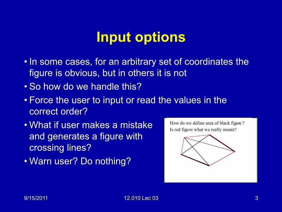
Input options • In some cases, for an arbitrary set of coordinates the

figure is obvious, but in others it is not • So how do we handle this? • Force the user to input or read the values in the

correct order? • What if user makes a mistake

and generates a figure with crossing lines?

• Warn user? Do nothing?

How do we define area of black figure ?

Is red figure what we really meant?

9/15/2011 12.010 Lec 03 4

Input options for Polygon • By considering scenarios before hand we can make a

robust program. • Inside your program and in documentation you

describe what you have decided to assume • You may also leave "place-holders" for features that

you may add later – not everything needs to be done in the first release.

• Final input option: Ask user number of points that will be entered? Or read list until End-of-file?

• Maximum number of points user can enter

9/15/2011 12.010 Lec 03 5

Calculation of area • Option 1: Area = base*height/2

– Base compute by Pythagoras theorem; height some method

• Option 2: Cross product: form triangle by two vectors and magnitude of cross product is twice the area

• This sounds appealing since forming vectors is easy and forming magnitude of cross product is easy

• If we decide to go with option 2, then this sets how we will form the triangles.

9/15/2011 12.010 Lec 03 6

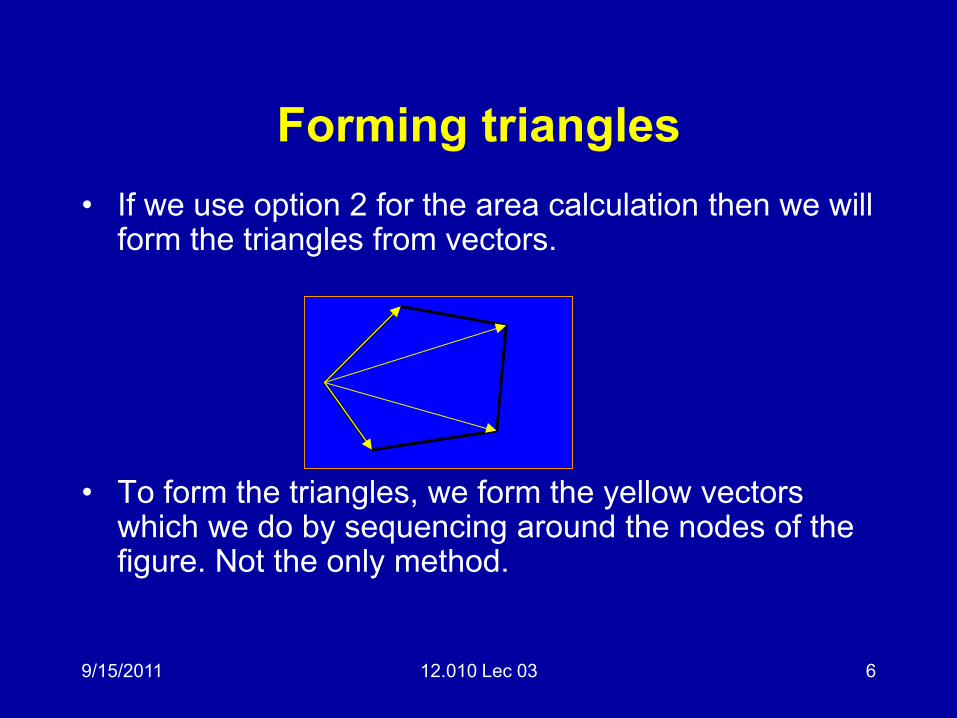
Forming triangles • If we use option 2 for the area calculation then we will

form the triangles from vectors.

• To form the triangles, we form the yellow vectors which we do by sequencing around the nodes of the figure. Not the only method.

9/15/2011 12.010 Lec 03 7

Output • Mainly we need to report the area. What units will say

the area is in? Need to ask user at being what the coordinate units are (e.g., m, km etc).

• Should we tell the user if lines cross? • Anything we have forgotten? • So we have now designed the basic algorithms we will

use, now we need to implement.

9/15/2011 12.010 Lec 03 8

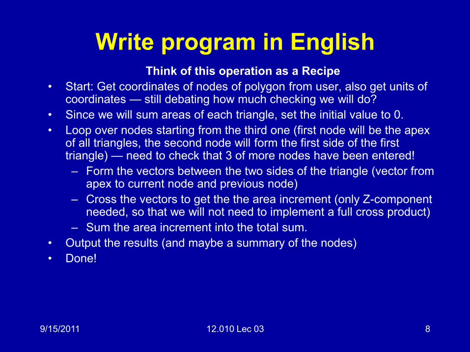
Write program in English Think of this operation as a Recipe

• Start: Get coordinates of nodes of polygon from user, also get units of coordinates — still debating how much checking we will do?

• Since we will sum areas of each triangle, set the initial value to 0. • Loop over nodes starting from the third one (first node will be the apex

of all triangles, the second node will form the first side of the first triangle) — need to check that 3 of more nodes have been entered! – Form the vectors between the two sides of the triangle (vector from

apex to current node and previous node) – Cross the vectors to get the the area increment (only Z-component

needed, so that we will not need to implement a full cross product) – Sum the area increment into the total sum.

• Output the results (and maybe a summary of the nodes) • Done!

9/15/2011 12.010 Lec 03 9

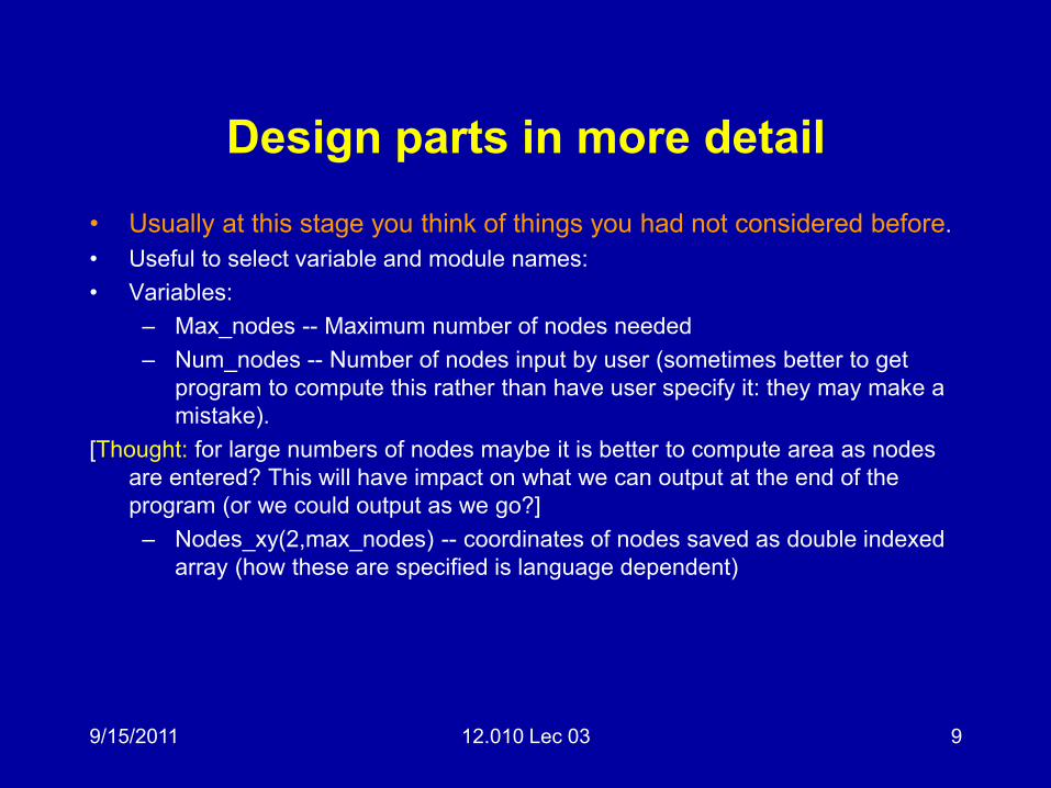
Design parts in more detail • Usually at this stage you think of things you had not considered before. • Useful to select variable and module names: • Variables:

– Max_nodes -- Maximum number of nodes needed – Num_nodes -- Number of nodes input by user (sometimes better to get

program to compute this rather than have user specify it: they may make a mistake).

[Thought: for large numbers of nodes maybe it is better to compute area as nodes are entered? This will have impact on what we can output at the end of the program (or we could output as we go?]

– Nodes_xy(2,max_nodes) -- coordinates of nodes saved as double indexed array (how these are specified is language dependent)

9/15/2011 12.010 Lec 03 10

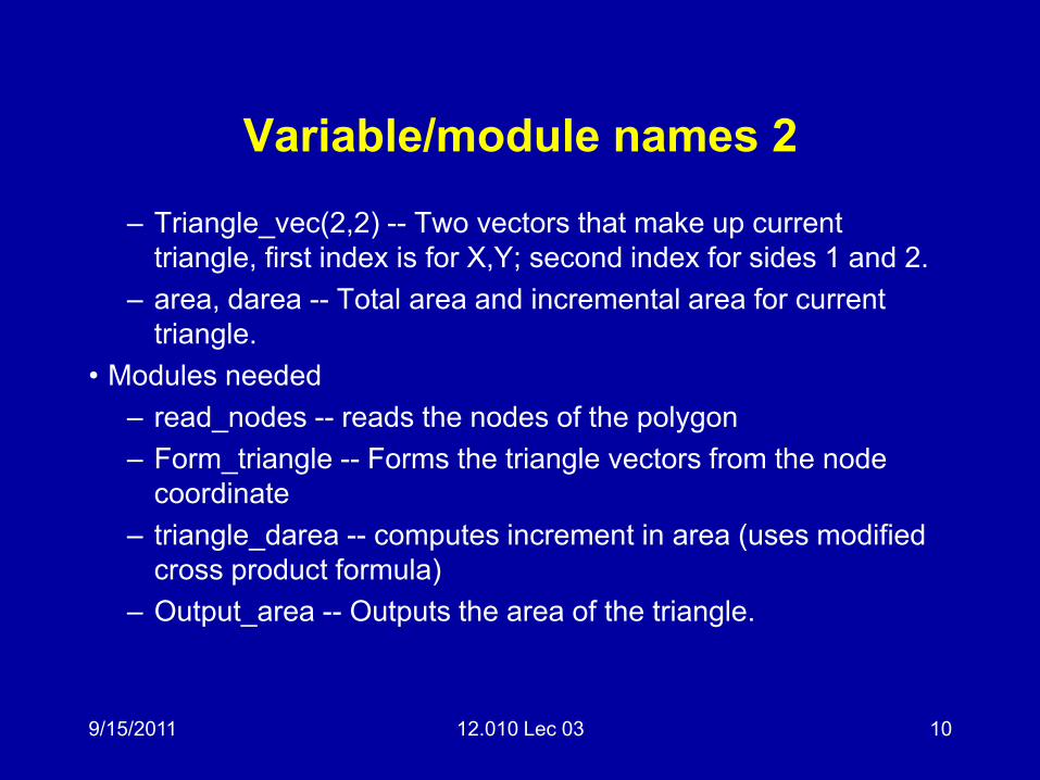
Variable/module names 2

– Triangle_vec(2,2) -- Two vectors that make up current triangle, first index is for X,Y; second index for sides 1 and 2.

– area, darea -- Total area and incremental area for current triangle.

• Modules needed – read_nodes -- reads the nodes of the polygon – Form_triangle -- Forms the triangle vectors from the node

coordinate – triangle_darea -- computes increment in area (uses modified

cross product formula) – Output_area -- Outputs the area of the triangle.

9/15/2011 12.010 Lec 03 11

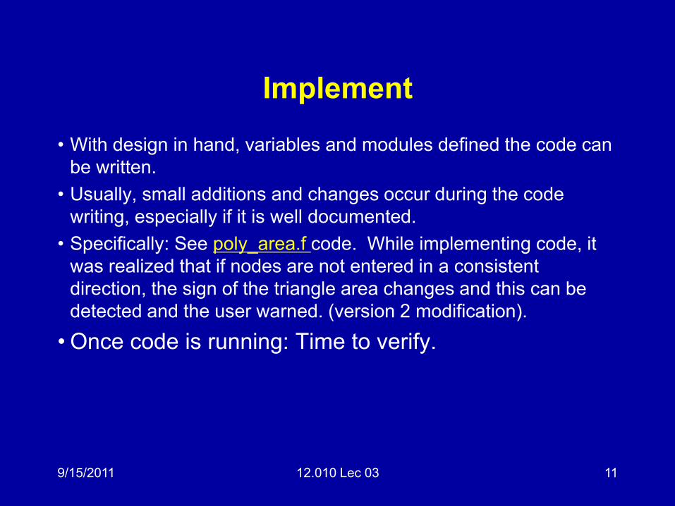
Implement

• With design in hand, variables and modules defined the code can be written.

• Usually, small additions and changes occur during the code writing, especially if it is well documented.

• Specifically: See poly_area.f code. While implementing code, it was realized that if nodes are not entered in a consistent direction, the sign of the triangle area changes and this can be detected and the user warned. (version 2 modification).

• Once code is running: Time to verify.

9/15/2011 12.010 Lec 03 12

Verification • Once code is implemented and running verification

can be done a number of ways. • Each module can be checked separately to ensure

that it works. Especially check the error treatment routines to make sure that they work.

• One then tests with selected examples where the results are known.

9/15/2011 12.010 Lec 03 13

Examine the program poly_area.f • Implementation of algorithm described above. • Take note of documentation • Checks on human input • This program will be looked in more detail when we

cover Fortran. • http://geoweb.mit.edu/~tah/12.010/poly_area.f

9/15/2011 12.010 Lec 03 14

Common problems • Numerical problems. Specifically

• Adding large and small numbers • Mixed type computations (i.e., integers, 4-byte and

8-byte floating point) • Division by zero. Generate not-a-number (Inf) on

many machines • Square root of a negative number (Not-a-Number,

NaN) • Values which should sum to zero but can be slightly

negative.

9/15/2011 12.010 Lec 03 15

Common problems 02 • Trigonometric functions computed low gradient points

[e.g., cos-1(~1), tan(~p)] • Quadrants of trigonometric functions

– For angle return, best to compute sin and cosine independently and use two-argument tan -1.

• Wrong units on functions (e.g., degrees instead of radians)

• Exceeding the bounds of memory and arrays. • Infinite loops (waiting for an input that will never come

or miscoding the exit) • Unexpected input that is not checked.

9/15/2011 12.010 Lec 03 16

Reading other’s code • Often you will asked to existing software and add

features to it • You should apply the techniques described in normal

program development to "reverse engineer" the program

• Specifically look for failure modes that you might fall into as you modify code (see check in form_triangles routine.

9/15/2011 12.010 Lec 03 17

Start of Fortran • Start examining the FORTRAN language • Development of the language • "Philosophy" of language: Why is FORTRAN still used

(other than you can’t teach an old dog new tricks) • Basic structure of its commands • Communications inside a program and with users • Next lecture will go into commands in more detail • There are many books on Fortran and an on-line

reference manual at: http://www.fortran.com/fortran/F77_std/rjcnf0001.html

9/15/2011 12.010 Lec 03 18

FORTRAN (Formula Translation).

• History – Developed between 1954-1957 at IBM – FORTRAN II released in 1958 – FORTRAN IV released in 1962 (standard for next 15 years) – FORTRAN 66 ANSI standard (basically FORTRAN IV). – FORTRAN 77 standard in 1977 – Fortran 90 Added new features, in 1997 Fortran 95 released

(started phasing out some FORTRAN 77 features). – Fortran 2000 and 2008 have been released but we will not

cover here.

9/15/2011 12.010 Lec 03 19

FORTRAN Philosophy • FORTRAN developed a time when computers needed

to do numerical calculations. • Its design is based on the idea of having modules

(subroutines and functions) that do calculations with variables (that contain numeric values) and to return the results of those calculations.

• FORTRAN programs are a series of modules that do calculations with typically the results of one module passed to the next.

• Usually programs need some type of IO to get values to computations with and to return the results.

9/15/2011 12.010 Lec 03 20

FORTRAN 77: • Commands are divided into executable and non-executable

ones. All non-executable commands must appear before the executable ones.

• Between commands, lines that start with C,* or ! are considered "comments" and are ignored

• Syntax is quite rigid (discuss later) • Basic Structure:

– Module types: • Program (only one per program, optional) • Subroutine — Multi-argument return • Function —single return (although not forced) • Block data —discuss later

9/15/2011 12.010 Lec 03 21

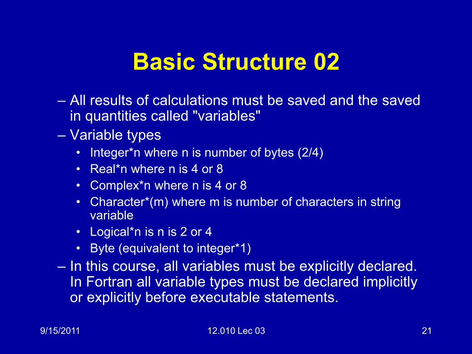
Basic Structure 02 – All results of calculations must be saved and the saved

in quantities called "variables" – Variable types

• Integer*n where n is number of bytes (2/4) • Real*n where n is 4 or 8 • Complex*n where n is 4 or 8 • Character*(m) where m is number of characters in string

variable • Logical*n is n is 2 or 4 • Byte (equivalent to integer*1)

– In this course, all variables must be explicitly declared. In Fortran all variable types must be declared implicitly or explicitly before executable statements.

9/15/2011 12.010 Lec 03 22

Basic Structure 03

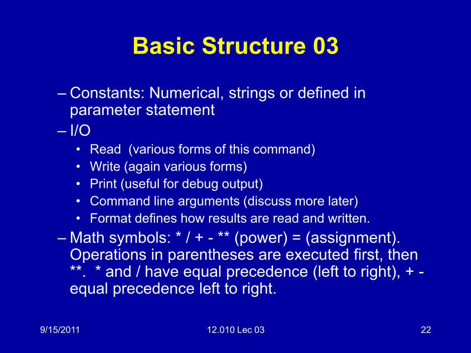
– Constants: Numerical, strings or defined in parameter statement

– I/O • Read (various forms of this command) • Write (again various forms) • Print (useful for debug output) • Command line arguments (discuss more later) • Format defines how results are read and written.

– Math symbols: * / + - ** (power) = (assignment). Operations in parentheses are executed first, then **. * and / have equal precedence (left to right), + - equal precedence left to right.

9/15/2011 12.010 Lec 03 23

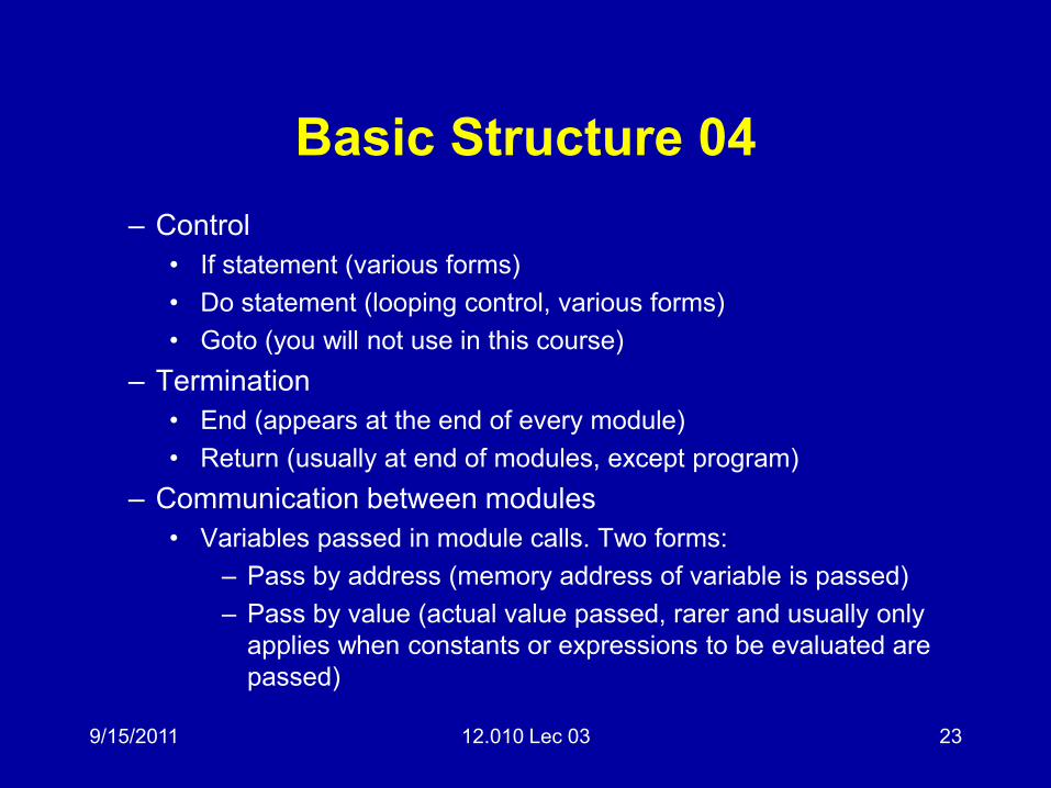
Basic Structure 04 – Control

• If statement (various forms) • Do statement (looping control, various forms) • Goto (you will not use in this course)

– Termination • End (appears at the end of every module) • Return (usually at end of modules, except program)

– Communication between modules • Variables passed in module calls. Two forms:

– Pass by address (memory address of variable is passed) – Pass by value (actual value passed, rarer and usually only

applies when constants or expressions to be evaluated are passed)

9/15/2011 12.010 Lec 03 24

Summary • Look at the basic characteristics of FORTRAN • Next lecture we look in more details of the syntax of

the commands (e.g., the arguments that can be used with an open statement)

• Trial FORTRAN programs will also be shown to examine the actual structure of a program.

MIT OpenCourseWarehttp://ocw.mit.edu

12.010 Computational Methods of Scientific ProgrammingFall 2011

For information about citing these materials or our Terms of Use, visit: http://ocw.mit.edu/terms.