Embed Size (px)
Citation preview
Vector-Valued Functions 12
Copyright © Cengage Learning. All rights reserved.
Vector-Valued Functions
Copyright © Cengage Learning. All rights reserved.
12.1
3
! Analyze and sketch a space curve given by a vector-valued function.
! Extend the concepts of limits and continuity to vector-valued functions.
Objectives
4
Space Curves and Vector-Valued Functions
5
Space Curves and Vector-Valued Functions
A plane curve is defined as the set of ordered pairs (f(t), g(t)) together with their defining parametric equations
x = f(t) and y = g(t)
where f and g are continuous functions of t on an interval I.
6
This definition can be extended naturally to three-dimensional space as follows.
A space curve C is the set of all ordered triples (f(t), g(t), h(t)) together with their defining parametric equations
x = f(t), y = g(t), and z = h(t)
where f, g and h are continuous functions of t on an interval I.
A new type of function, called a vector-valued function, is introduced. This type of function maps real numbers to vectors.
Space Curves and Vector-Valued Functions
7
A
Space Curves and Vector-Valued Functions
8
Technically, a curve in the plane or in space consists of a collection of points and the defining parametric equations.
Two different curves can have the same graph.
For instance, each of the curves given by
r(t) = sin t i + cos t j and r(t) = sin t2 i + cos t2 j
has the unit circle as its graph, but these equations do not represent the same curve—because the circle is traced out in different ways on the graphs.
Space Curves and Vector-Valued Functions
9
Be sure you see the distinction between the vector-valued function r and the real-valued functions f, g, and h.
All are functions of the real variable t, but r(t) is a vector, whereas f(t), g(t), and h(t) are real numbers (for each specific value of t).
Space Curves and Vector-Valued Functions
10
Vector-valued functions serve dual roles in the representation of curves.
By letting the parameter t represent time, you can use a vector-valued function to represent motion along a curve.
Or, in the more general case, you can use a vector-valued function to trace the graph of a curve.
Space Curves and Vector-Valued Functions
11
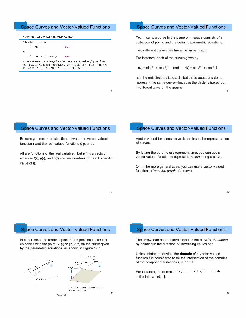
In either case, the terminal point of the position vector r(t) coincides with the point (x, y) or (x, y, z) on the curve given by the parametric equations, as shown in Figure 12.1.
Figure 12.1
Space Curves and Vector-Valued Functions
12
The arrowhead on the curve indicates the curve’s orientation by pointing in the direction of increasing values of t.
Unless stated otherwise, the domain of a vector-valued function r is considered to be the intersection of the domains of the component functions f, g, and h.
For instance, the domain of is the interval (0, 1].
Space Curves and Vector-Valued Functions
13
Sketch the plane curve represented by the vector-valued function r(t) = 2cos t i – 3sin t j, 0 ! t ! 2!. Vector-valued function
Solution: From the position vector r(t), you can write the parametric equations x = 2cos t and y = –3sin t.
Solving for cos t and sin t and using the identity cos2 t + sin2 t = 1 produces the rectangular equation
Rectangular equation
Example 1 – Sketching a Plane Curve
14
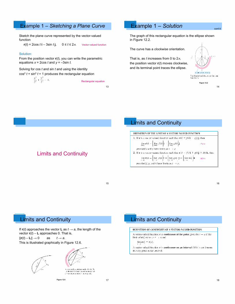
The graph of this rectangular equation is the ellipse shown in Figure 12.2.
The curve has a clockwise orientation.
That is, as t increases from 0 to 2!, the position vector r(t) moves clockwise, and its terminal point traces the ellipse.
Figure 12.2
cont’d Example 1 – Solution
15
Limits and Continuity
16
Limits and Continuity
17
If r(t) approaches the vector L as t " a, the length of the vector r(t) – L approaches 0. That is, ||r(t) – L|| " 0 as t " a. This is illustrated graphically in Figure 12.6.
Figure 12.6
Limits and Continuity
18
Limits and Continuity
19
Discuss the continuity of the vector-valued function given by r(t) = ti + aj + (a2 – t2)k a is a constant.
at t = 0.
Solution: As t approaches 0, the limit is
Example 5 – Continuity of Vector-Valued Functions
20
Because
r(0) = (0)i + (a)j + (a2)k = aj + a2k
you can conclude that r is continuous at t = 0.
By similar reasoning, you can conclude that the vector-valued function r is continuous at all real-number values of t.
Example 5 – Solution cont’d
21
Differentiation and Integration of Vector-Valued Functions
Copyright © Cengage Learning. All rights reserved.
12.2
22
! Differentiate a vector-valued function.
! Integrate a vector-valued function.
Objectives
23
Differentiation of Vector-Valued Functions
24
Differentiation of Vector-Valued Functions
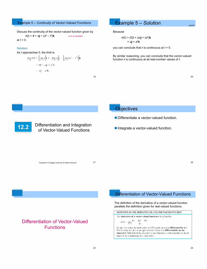
The definition of the derivative of a vector-valued function parallels the definition given for real-valued functions.
25
Differentiation of Vector-Valued Functions
Differentiation of vector-valued functions can be done on a component-by-component basis.
To see why this is true, consider the function given by r(t) = f(t)i + g(t)j.
26
Differentiation of Vector-Valued Functions
Applying the definition of the derivative produces the following.
This important result is listed in the theorem 12.1.
27
Note that the derivative of the vector-valued function r is itself a vector-valued function.
You can see from Figure 12.8 that r#(t) is a vector tangent to the curve given by r(t) and pointing in the direction of increasing t-values.
Figure 12.8
Differentiation of Vector-Valued Functions
28
Differentiation of Vector-Valued Functions
29
Example 1 – Differentiation of Vector-Valued Functions
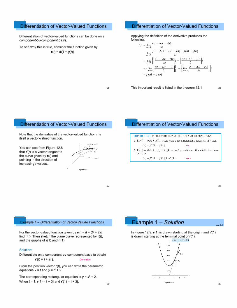
For the vector-valued function given by r(t) = ti + (t2 + 2)j, find r#(t). Then sketch the plane curve represented by r(t), and the graphs of r(1) and r#(1).
Solution: Differentiate on a component-by-component basis to obtain
r#(t) = i + 2t j. Derivative
From the position vector r(t), you can write the parametric equations x = t and y = t2 + 2.
The corresponding rectangular equation is y = x2 + 2. When t = 1, r(1) = i + 3j and r#(1) = i + 2j.
30
Example 1 – Solution
In Figure 12.9, r(1) is drawn starting at the origin, and r#(1) is drawn starting at the terminal point of r(1).
Figure 12.9
cont’d
31
Differentiation of Vector-Valued Functions
The parametrization of the curve represented by the vector-valued function
r(t) = f(t)i + g(t)j + h(t)k is smooth on an open interval " if f#, g#, and h# are continuous on " and r#(t) $ 0 for any value of t in the interval ".
32
Example 3 – Finding Intervals on Which a Curve Is Smooth
Find the intervals on which the epicycloid C given by r(t) = (5cos t – cos 5t)i + (5sin t – sin 5t)j, 0 ! t ! 2! is smooth.
Solution:
The derivative of r is
r#(t) = (–5sin t + 5sin 5t)i + (5cos t – 5cos 5t)j.
In the interval [0, 2!], the only values of t for which
r#(t) = 0i + 0j are t = 0, !/2, !, 3!/2, and 2!.
33
Example 3 – Solution
Therefore, you can conclude that C is smooth in the intervals
as shown in Figure 12.10.
In Figure 12.10, note that the curve is not smooth at points at which the curve makes abrupt changes in direction.
Such points are called cusps or nodes.
Figure 12.10
cont’d
34
Differentiation of Vector-Valued Functions
35
Example 4 – Using Properties of the Derivative
For the vector-valued functions given by
find
a. Dt[r(t) . u(t)]
and
b. Dt[u(t) " u#(t)].
36
Example 4(a) – Solution
Because and u#(t) = 2ti – 2j, you have
37
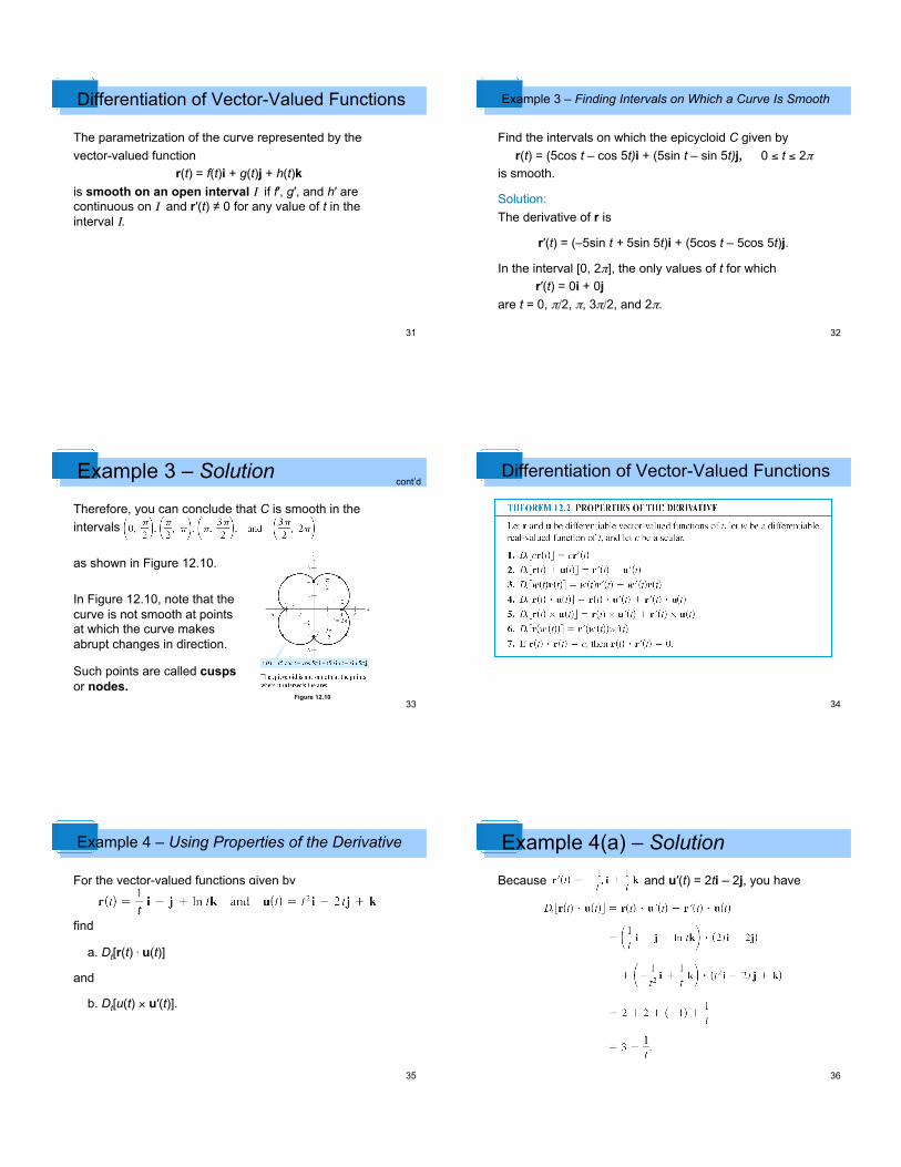
Example 4(b) – Solution
Because u#(t) = 2ti – 2j and u##(t) = 2i, you have
cont’d
38
Integration of Vector-Valued Functions
39
Integration of Vector-Valued Functions
The following definition is a rational consequence of the definition of the derivative of a vector-valued function.
40
The antiderivative of a vector-valued function is a family of vector-valued functions all differing by a constant vector C.
For instance, if r(t) is a three-dimensional vector-valued function, then for the indefinite integral !r(t) dt, you obtain three constants of integration
where F!(t) = f(t), G!(t) = g(t), and H!(t) = h(t). These three scalar constants produce one vector constant of integration, !r(t) dt = [F(t) + C1]i + [G(t) + C2]j + [H(t) + C3]k
Integration of Vector-Valued Functions
41
= [F(t)i + G(t)j + H(t)k] + [C1i + C2 j + C3k] = R(t) + C
where R"(t) = r(t).
Integration of Vector-Valued Functions
42
Example 5 – Integrating a Vector-Valued Function
Find the indefinite integral !(t i + 3j) dt.
Solution: Integrating on a component-by-component basis produces
43
Velocity and Acceleration
Copyright © Cengage Learning. All rights reserved.
12.3
44
! Describe the velocity and acceleration associated with a vector-valued function.
! Use a vector-valued function to analyze projectile motion.
Objectives
45
Velocity and Acceleration
46
Velocity and Acceleration
As an object moves along a curve in the plane, the coordinates x and y of its center of mass are each functions of time t.
Rather than using the letters f and g to represent these two functions, it is convenient to write x = x(t) and y = y(t).
So, the position vector r(t) takes the form r(t) = x(t)i + y(t)j.
47
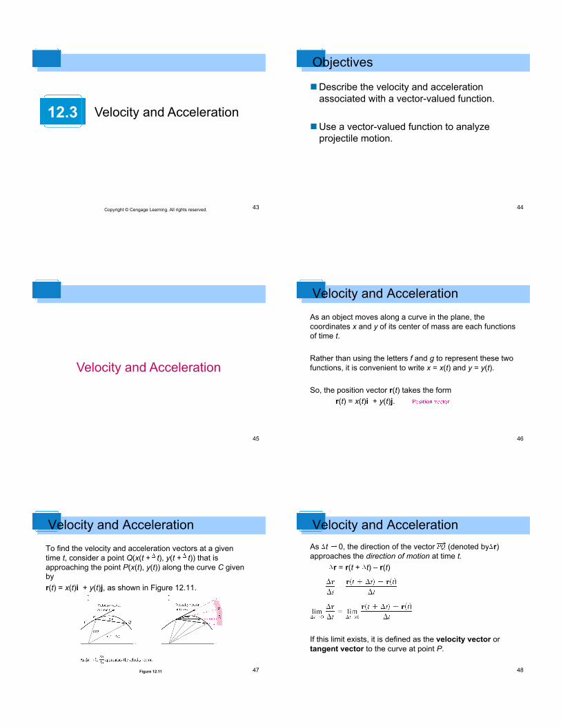
To find the velocity and acceleration vectors at a given time t, consider a point Q(x(t + t), y(t + t)) that is approaching the point P(x(t), y(t)) along the curve C given by r(t) = x(t)i + y(t)j, as shown in Figure 12.11.
Figure 12.11
Velocity and Acceleration
48
As t 0, the direction of the vector (denoted by r) approaches the direction of motion at time t. r = r(t + t) – r(t)
If this limit exists, it is defined as the velocity vector or tangent vector to the curve at point P.
Velocity and Acceleration
49
Note that this is the same limit used to define r'(t). So, the direction of r'(t) gives the direction of motion at time t.
Moreover, the magnitude of the vector r'(t)
gives the speed of the object at time t.
Similarly, you can use r''(t) to find acceleration.
Velocity and Acceleration
50
Velocity and Acceleration
51
For motion along a space curve, the definitions are similar.
That is, if r(t) = x(t)i + y(t)j + z(t)k, you have
Velocity = v(t) = r'(t) = x'(t)i + y'(t)j + z'(t)k
Acceleration = a(t) = r''(t) = x''(t)i + y''(t)j + z''(t)k
Speed =
Velocity and Acceleration
52
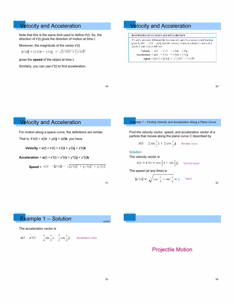
Find the velocity vector, speed, and acceleration vector of a particle that moves along the plane curve C described by
Solution: The velocity vector is
The speed (at any time) is
Example 1 – Finding Velocity and Acceleration Along a Plane Curve
53
The acceleration vector is
Example 1 – Solution cont’d
54
Projectile Motion
55
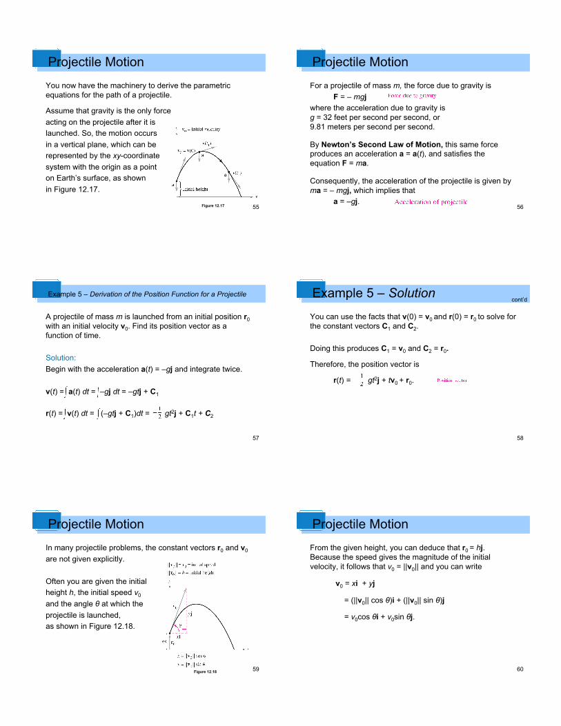
You now have the machinery to derive the parametric equations for the path of a projectile.
Assume that gravity is the only force acting on the projectile after it is launched. So, the motion occurs in a vertical plane, which can be represented by the xy-coordinate system with the origin as a point on Earth’s surface, as shown in Figure 12.17.
Figure 12.17
Projectile Motion
56
For a projectile of mass m, the force due to gravity is F = – mgj
where the acceleration due to gravity is g = 32 feet per second per second, or 9.81 meters per second per second.
By Newton’s Second Law of Motion, this same force produces an acceleration a = a(t), and satisfies the equation F = ma.
Consequently, the acceleration of the projectile is given by ma = – mgj, which implies that
a = –gj.
Projectile Motion
57
A projectile of mass m is launched from an initial position r0 with an initial velocity v0. Find its position vector as a function of time.
Solution: Begin with the acceleration a(t) = –gj and integrate twice.
v(t) = a(t) dt = –gj dt = –gtj + C1
r(t) = v(t) dt = (–gtj + C1)dt = gt2j + C1t + C2
Example 5 – Derivation of the Position Function for a Projectile
58
You can use the facts that v(0) = v0 and r(0) = r0 to solve for the constant vectors C1 and C2.
Doing this produces C1 = v0 and C2 = r0.
Therefore, the position vector is
r(t) = gt2j + tv0 + r0.
Example 5 – Solution cont’d
59 Figure 12.18
In many projectile problems, the constant vectors r0 and v0 are not given explicitly.
Often you are given the initial height h, the initial speed v0 and the angle " at which the projectile is launched, as shown in Figure 12.18.
Projectile Motion
60
From the given height, you can deduce that r0 = hj. Because the speed gives the magnitude of the initial velocity, it follows that v0 = ||v0|| and you can write
v0 = xi + yj
= (||v0|| cos ")i + (||v0|| sin ")j
= v0cos "i + v0sin "j.
Projectile Motion
61
So, the position vector can be written in the form
= gt2j + tv0cos "i + tv0sin "j + hj
= (v0cos ")ti +
Projectile Motion
62
Projectile Motion
63
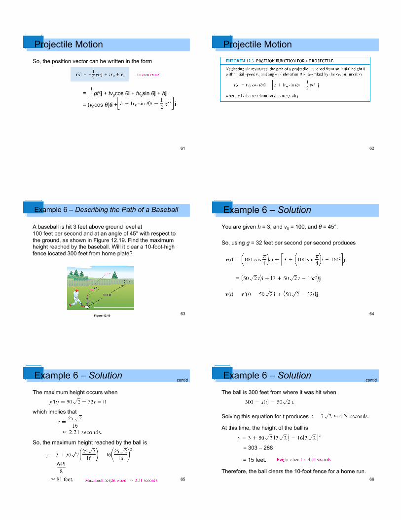
A baseball is hit 3 feet above ground level at 100 feet per second and at an angle of 45° with respect to the ground, as shown in Figure 12.19. Find the maximum height reached by the baseball. Will it clear a 10-foot-high fence located 300 feet from home plate?
Example 6 – Describing the Path of a Baseball
Figure 12.19 64
You are given h = 3, and v0 = 100, and " = 45°.
So, using g = 32 feet per second per second produces
Example 6 – Solution
65
The maximum height occurs when
which implies that
So, the maximum height reached by the ball is
Example 6 – Solution cont’d
66
The ball is 300 feet from where it was hit when
Solving this equation for t produces
At this time, the height of the ball is
= 303 – 288
= 15 feet.
Therefore, the ball clears the 10-foot fence for a home run.
Example 6 – Solution cont’d
67
Tangent Vectors and Normal Vectors
Copyright © Cengage Learning. All rights reserved.
12.4
68
! Find a unit tangent vector at a point on a space curve.
! Find the tangential and normal components of acceleration.
Objectives
69
Tangent Vectors and Normal Vectors
70
Tangent Vectors and Normal Vectors
71
Example 1 – Finding the Unit Tangent Vector
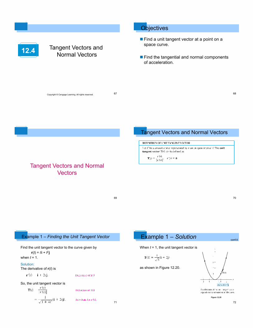
Find the unit tangent vector to the curve given by r(t) = t i + t2 j when t = 1.
Solution: The derivative of r(t) is
So, the unit tangent vector is
72
Example 1 – Solution
When t = 1, the unit tangent vector is
as shown in Figure 12.20.
Figure 12.20
cont’d

73
The tangent line to a curve at a point is the line that passes through the point and is parallel to the unit tangent vector.
Tangent Vectors and Normal Vectors
74
Example 2 – Finding the Tangent Line at a Point on a Curve
Find T(t) and then find a set of parametric equations for the tangent line to the helix given by r(t) = 2cos t i + 2sin t j + t k
at the point
Solution: The derivative of r(t) is r'(t) = –2sin t i + 2cos t j + k, which implies that
Therefore, the unit tangent vector is
75
Example 2 – Solution
At the point and the unit tangent vector is
cont’d
76
Using the direction numbers and the point you can obtain the following parametric equations (given with parameter s).
Example 2 – Solution cont’d
77 Figure 12.21
This tangent line is shown in Figure 12.21.
Example 2 – Solution cont’d
78
In Example 2, there are infinitely many vectors that are orthogonal to the tangent vector T(t). One of these is the vector T'(t) . This follows the property
T(t) ! T(t) = ||T(t)||2 =1 T(t) ! T'(t) = 0
By normalizing the vector T'(t) , you obtain a special vector called the principal unit normal vector, as indicated in the following definition.
Tangent Vectors and Normal Vectors
79
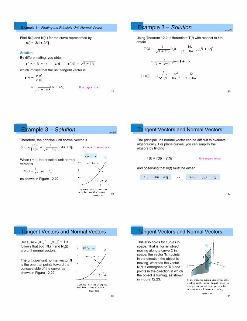
Example 3 – Finding the Principle Unit Normal Vector
Find N(t) and N(1) for the curve represented by r(t) = 3t i + 2t2 j.
Solution: By differentiating, you obtain
which implies that the unit tangent vector is
80
Example 3 – Solution
Using Theorem 12.2, differentiate T(t) with respect to t to obtain
cont’d
81
Therefore, the principal unit normal vector is
When t = 1, the principal unit normal vector is
as shown in Figure 12.22.
Figure 12.22
Example 3 – Solution cont’d
82
The principal unit normal vector can be difficult to evaluate algebraically. For plane curves, you can simplify the algebra by finding
T(t) = x(t)i + y(t)j Unit tangent vector
and observing that N(t) must be either
Tangent Vectors and Normal Vectors
83
Because it follows that both N1(t) and N2(t) are unit normal vectors.
The principal unit normal vector N is the one that points toward the concave side of the curve, as shown in Figure 12.22
Figure 12.22
Tangent Vectors and Normal Vectors
84
This also holds for curves in space. That is, for an object moving along a curve C in space, the vector T(t) points in the direction the object is moving, whereas the vector N(t) is orthogonal to T(t) and points in the direction in which the object is turning, as shown in Figure 12.23.
Figure 12.23
Tangent Vectors and Normal Vectors
85
Tangential and Normal Components of Acceleration
86
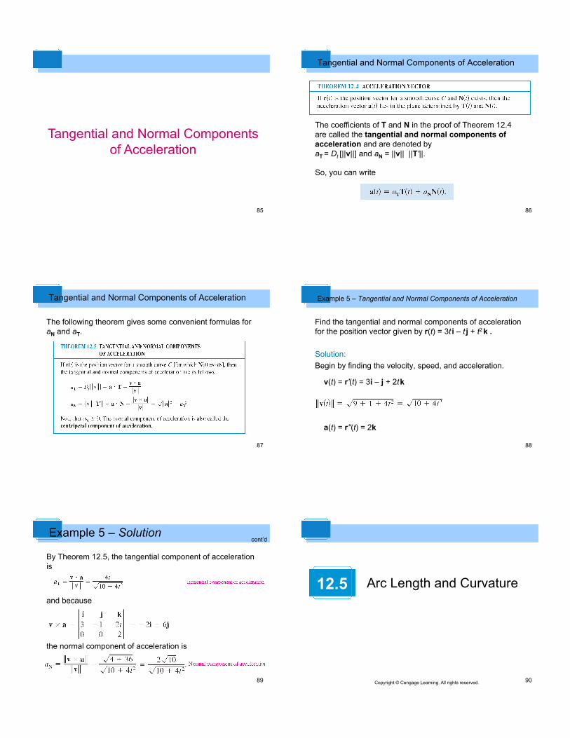
The coefficients of T and N in the proof of Theorem 12.4 are called the tangential and normal components of acceleration and are denoted by aT = Dt [||v||] and aN = ||v|| ||T'||.
So, you can write
Tangential and Normal Components of Acceleration
87
The following theorem gives some convenient formulas for aN and aT.
Tangential and Normal Components of Acceleration
88
Example 5 – Tangential and Normal Components of Acceleration
Find the tangential and normal components of acceleration for the position vector given by r(t) = 3t i – t j + t2 k .
Solution: Begin by finding the velocity, speed, and acceleration.
v(t) = r'(t) = 3i – j + 2t k
a(t) = r''(t) = 2k
89
Example 5 – Solution
By Theorem 12.5, the tangential component of acceleration is
and because
the normal component of acceleration is
cont’d
90
Arc Length and Curvature
Copyright © Cengage Learning. All rights reserved.
12.5
91
! Find the arc length of a space curve.
! Use the arc length parameter to describe a plane curve or space curve.
! Find the curvature of a curve at a point on the curve.
! Use a vector-valued function to find frictional force.
Objectives
92
Arc Length
93
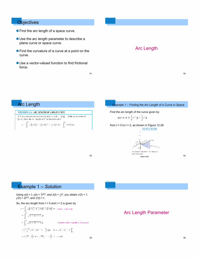
Arc Length
94
Find the arc length of the curve given by
from t = 0 to t = 2, as shown in Figure 12.28.
Example 1 – Finding the Arc Length of a Curve in Space
Figure 12.28
95
Using x(t) = t, y(t) = t3/2, and z(t) = t2, you obtain x!(t) = 1, y!(t) = 2t1/2, and z!(t) = t.
So, the arc length from t = 0 and t = 2 is given by
Example 1 – Solution
96
Arc Length Parameter
97
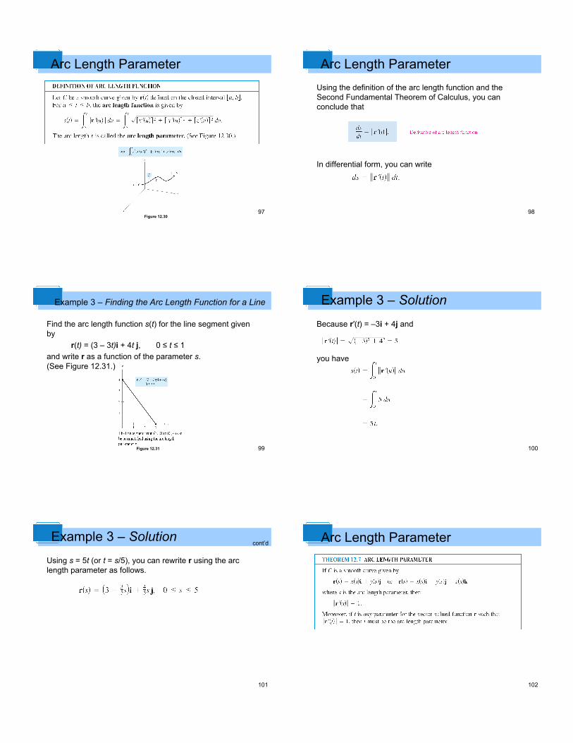
Arc Length Parameter
Figure 12.30 98
Using the definition of the arc length function and the Second Fundamental Theorem of Calculus, you can conclude that
In differential form, you can write
Arc Length Parameter
99
Find the arc length function s(t) for the line segment given by r(t) = (3 – 3t)i + 4t j, 0 ! t ! 1 and write r as a function of the parameter s. (See Figure 12.31.)
Example 3 – Finding the Arc Length Function for a Line
Figure 12.31 100
Because r#(t) = –3i + 4j and
you have
Example 3 – Solution
101
Using s = 5t (or t = s/5), you can rewrite r using the arc length parameter as follows.
Example 3 – Solution cont’d
102
Arc Length Parameter
103
Curvature
104
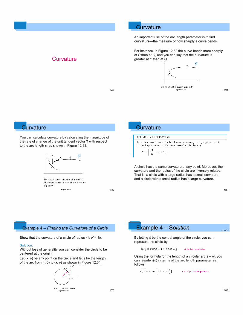
An important use of the arc length parameter is to find curvature—the measure of how sharply a curve bends.
For instance, in Figure 12.32 the curve bends more sharply at P than at Q, and you can say that the curvature is greater at P than at Q.
Curvature
Figure 12.32
105
You can calculate curvature by calculating the magnitude of the rate of change of the unit tangent vector T with respect to the arc length s, as shown in Figure 12.33.
Curvature
Figure 12.33 106
A circle has the same curvature at any point. Moreover, the curvature and the radius of the circle are inversely related. That is, a circle with a large radius has a small curvature, and a circle with a small radius has a large curvature.
Curvature
107 Figure 12.34
Show that the curvature of a circle of radius r is K = 1/r.
Solution: Without loss of generality you can consider the circle to be centered at the origin. Let (x, y) be any point on the circle and let s be the length of the arc from (r, 0) to (x, y) as shown in Figure 12.34.
Example 4 – Finding the Curvature of a Circle
108
By letting # be the central angle of the circle, you can represent the circle by
r(#) = r cos # i + r sin # j. # is the parameter.
Using the formula for the length of a circular arc s = r#, you can rewrite r(#) in terms of the arc length parameter as follows.
Example 4 – Solution cont’d

109
So, , and it follows that , which implies that the unit tangent vector is
and the curvature is given by
at every point on the circle.
Example 4 – Solution cont’d
110
Because , the first formula implies that curvature is the ratio of the rate of change in the tangent vector T to the rate of change in arc length. To see that this is reasonable, let #t be a “small number.” Then,
Curvature
111
In other words, for a given #s, the greater the length of #T, the more the curve bends at t, as shown in Figure 12.35.
Curvature
Figure 12.35
112
Find the curvature of the curve given by
Solution: It is not apparent whether this parameter represents arc length, so you should use the formula
r#(t) = 2i + 2t j – t2k
Example 5 – Finding the Curvature of a Space Curve
113
Therefore,
Example 5 – Solution cont’d
114
Curvature
115
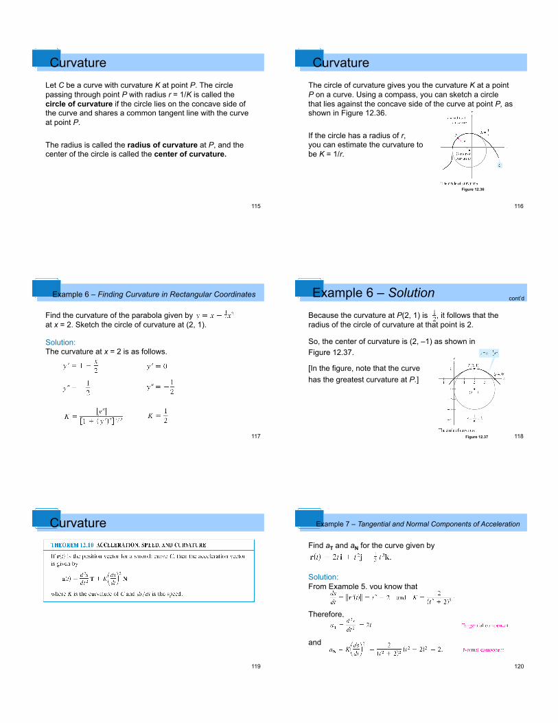
Let C be a curve with curvature K at point P. The circle passing through point P with radius r = 1/K is called the circle of curvature if the circle lies on the concave side of the curve and shares a common tangent line with the curve at point P.
The radius is called the radius of curvature at P, and the center of the circle is called the center of curvature.
Curvature
116
The circle of curvature gives you the curvature K at a point P on a curve. Using a compass, you can sketch a circle that lies against the concave side of the curve at point P, as shown in Figure 12.36.
If the circle has a radius of r, you can estimate the curvature to be K = 1/r.
Figure 12.36
Curvature
117
Find the curvature of the parabola given by at x = 2. Sketch the circle of curvature at (2, 1).
Solution: The curvature at x = 2 is as follows.
Example 6 – Finding Curvature in Rectangular Coordinates
118
Because the curvature at P(2, 1) is , it follows that the radius of the circle of curvature at that point is 2.
So, the center of curvature is (2, –1) as shown in Figure 12.37.
[In the figure, note that the curve has the greatest curvature at P.]
Example 6 – Solution
Figure 12.37
cont’d
119
Curvature
120
Find aT and aN for the curve given by
Solution: From Example 5, you know that
Therefore,
and
Example 7 – Tangential and Normal Components of Acceleration
121
Application
122
There are many applications in physics and engineering dynamics that involve the relationships among speed, arc length, curvature, and acceleration. One such application concerns frictional force.
A moving object with mass m is in contact with a stationary object. The total force required to produce an acceleration a along a given path is
The portion of this total force that is supplied by the stationary object is called the force of friction.
Application
123
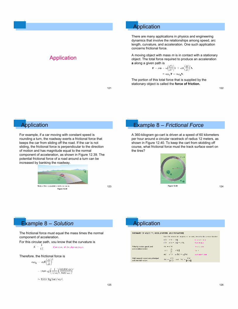
For example, if a car moving with constant speed is rounding a turn, the roadway exerts a frictional force that keeps the car from sliding off the road. If the car is not sliding, the frictional force is perpendicular to the direction of motion and has magnitude equal to the normal component of acceleration, as shown in Figure 12.39. The potential frictional force of a road around a turn can be increased by banking the roadway.
Application
Figure 12.39 124
A 360-kilogram go-cart is driven at a speed of 60 kilometers per hour around a circular racetrack of radius 12 meters, as shown in Figure 12.40. To keep the cart from skidding off course, what frictional force must the track surface exert on the tires?
Example 8 – Frictional Force
Figure 12.40
125
The frictional force must equal the mass times the normal component of acceleration. For this circular path, you know that the curvature is
Therefore, the frictional force is
Example 8 – Solution
126
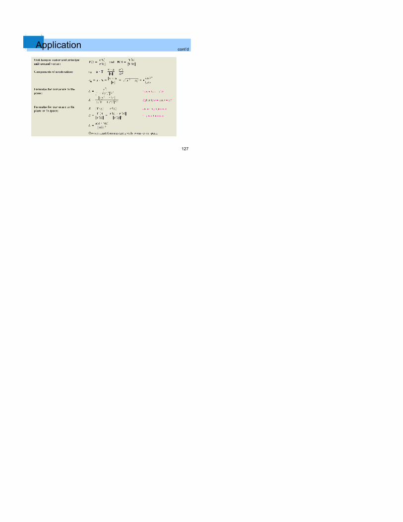
Application
127
Application cont’d