12 - Université de Nantes

DRAFT12

Informed learners

Understanding is compression, comprehension is compression!Greg Chaitin (Chaitin, 2007)

Comprendo. Habla de un juego donde las reglas no sean la líneade salida, sino el punto de llegada ¿No?

Arturo Pérez-Reverte, el pintor de batallas

‘Learning from an informant’ is the setting in which the data consists of labelled strings,each label indicating whether or not the string belongs to the target language.

Of all the issues which grammatical inference scientists have worked on, this is prob-ably the one on which most energy has been spent over the years. Algorithms have beenproposed, competitions have been launched, theoretical results have been given. On onehand, the problem has been proved to be on a par with mighty theoretical computer sci-ence questions arising from combinatorics, number theory and cryptography, and on theother hand cunning heuristics and techniques employing ideas from artificial intelligenceand language theory have been devised.

There would be a point in presenting this theme with a special focus on the class ofcontext-free grammars with a hope that the theory for the particular class of the finiteautomata would follow, but the history and the techniques tell us otherwise. The mainfocus is therefore going to be on the simpler yet sufficiently rich question of learningdeterministic finite automata from positive and negative examples.

We shall justify this as follows:

• On one hand the task is hard enough, and, through showing what doesn’t work and why, we willhave a precious insight into more complex classes.

• On the other hand anything useful learnt on DFAs can be nicely transferred thanks to reductions(see Chapter 7) to other supposedly richer classes.

• Finally, there are historical reasons: on the specific question of learning DFAs from an informedpresentation, some of the most important algorithms in grammatical inference have been invented,and many new ideas have been introduced due to this effort.

The specific question of learning context-free grammars and languages from an informantwill be studied as a separate problem, in Chapter 15.

237

DRAFT238 Informed learners

12.1 The prefix tree acceptor (PTA)

We shall be dealing here with learning samples composed of labelled strings:

Definition 12.1.1 Let � be an alphabet. An informed learning sample is made of twosets S+ and S− such that S+ ∩ S− = ∅. The sample will be denoted as S = 〈S+, S−〉.We will alternatively denote (x, 1) ∈ S for x ∈ S+ and (x, 0) ∈ S for x ∈ S−. LetA = 〈�, Q, qλ,FA,FR, δ〉 be a DFA.

Definition 12.1.2 A is weakly consistent with the sample S= 〈S+, S−〉 ifdef

∀x ∈ S+, δ(qλ, x) ∈ FA and ∀x ∈ S−, δ(qλ, x) �∈ FA.

Definition 12.1.3 A is strongly consistent with the sample S= 〈S+, S−〉 ifdef

∀x ∈ S+, δ(qλ, x) ∈ FA and ∀x ∈ S−, δ(qλ, x) ∈ FR.

Example 12.1.1 The DFA from Figure 12.1 is only weakly consistent with the sample{(aa, 1), (abb, 0), (b, 0)} which can also be denoted as:

S+ = {aa}S− = {abb,b}.

String abb ends in state qλ which is unlabelled (neither accepting nor rejecting), and stringb (from S−) cannot be entirely parsed. Therefore the DFA is not strongly consistent. Onthe other hand the same automaton can be shown to be strongly consistent with the sample{(aa, 1), (aba, 1)(abab, 0)}.

A prefix tree acceptor (PTA) is a tree-like DFA built from the learning sample by takingall the prefixes in the sample as states and constructing the smallest DFA which is a tree(∀q ∈ Q, | {q ′ : δ(q ′, a) = q}| ≤ 1}), strongly consistent with the sample. A formalalgorithm (BUILD-PTA) is given (Algorithm 12.1).

An example of a PTA is shown in Figure 12.2.Note that we can also build a PTA from a set of positive strings only. This corresponds

to building the PTA (〈S+,∅〉). In that case, for the same sample we would get the PTArepresented in Figure 12.3.

qλ

qa

qaa

qab

a a

b

a

b

b

a

Fig. 12.1. A DFA.

DRAFT12.1 The prefix tree acceptor (PTA) 239

Algorithm 12.1: BUILD-PTA.

Input: a sample 〈S+, S−〉Output: A = PTA(〈S+, S−〉) = 〈�, Q, qλ,FA,FR, δ〉FA ← ∅;FR ← ∅;Q ← {qu : u ∈ PREF(S+ ∪ S−)};for qu·a ∈ Q do δ(qu, a)← qua ;for qu ∈ Q do

if u ∈ S+ then FA ← FA ∪ {qu};if u ∈ S− then FR ← FR ∪ {qu}

endreturn A

qλ

qa

qb

qaa

qab

qbb

qaba

qbba

qabab

a

b

a

b

b

a b

a

Fig. 12.2. PTA ({(aa, 1), (aba, 1), (bba, 1), (ab, 0), (abab, 0)}).

qλ

qa

qb

qaa

qab

qbb

qaba

qbba

a

b

a

b

b

a

a

Fig. 12.3. PTA ({(aa, 1), (aba, 1), (bba, 1)}).

In Chapter 6 we will consider the problem of grammatical inference as the one ofsearching inside a space of admissible biased solutions, in which case we will introduce anon-deterministic version of the PTA.

Most algorithms will take the PTA as a starting point and try to generalise from itby merging states. In order not to get lost in the process (and not undo merges thathave been made some time ago) it will be interesting to divide the states into threecategories:


qλ

qa

qb

qaa

qab

qbb

qaba

qbba

qabab

a

b

a

b

b

a b

a

Fig. 12.4. Colouring of states: RED = {qλ, qa}, BLUE = {qb, qaa, qab}, and all theother states are WHITE.

qλ

qa

qaa

qab

a a

b

a

b

b

a

Fig. 12.5. The DFA Aqab .

• The RED states which correspond to states that have been analysed and which will not be revisited;they will be the states of the final automaton.

• The BLUE states which are the candidate states: they have not been analysed yet and it should befrom this set that a state is drawn in order to consider merging it with a RED state.

• The WHITE states, which are all the others. They will in turn become BLUE and then RED.

Example 12.1.2 We conventionally draw the RED states in dark grey and the BLUE onesin light grey as in Figure 12.4, where RED = {qλ, qa} and BLUE = {qb, qaa, qab}.We will need to describe the suffix language in any state q, consisting of the languagerecognised by the automaton when taking this state q as initial. We denote this automatonformally by Aq with L(Aq) = {w ∈ �� : δ(q, w) ∈ FA}. In Figure 12.5 we have used theautomaton A from Figure 12.1 and chosen state qab as initial.

12.2 The basic operations

We first describe some operations common to many of the state merging techniques. Statemerging techniques iteratively consider an automaton and two of its states and aim tomerge them. This will be done when these states are compatible. Sometimes, when notic-ing that a particular state cannot be merged, it gets promoted. Furthermore at any momentall states are either RED, BLUE or WHITE. Let us also suppose that the current automatonis consistent with the sample. The starting point is the prefix tree acceptor (PTA). Ini-tially, in the PTA, the unique RED state is qλ whereas the BLUE states are the immediatesuccessors of qλ.

DRAFT12.2 The basic operations 241

qλ qa qaaa a

(a) PTA({aa, 1), (λ, 0)}.

qλ qaa

a

a

(b) After merging qλ and qa.

qλ

a

(c) After mergingqλ, qa and qaa.

Fig. 12.6. Incompatibility is not a local affair.

There are three basic operations that shall be systematically used and need to be studiedindependently of the learning algorithms: COMPATIBLE, MERGE and PROMOTE.

12.2.1 COMPATIBLE: deciding equivalence between states

The question here is of deciding if two states are compatible or not. This is the same asdeciding equivalence for the Nerode relation, but with only partial knowledge about thelanguage. As obviously we do not have the entire language to help us decide upon this, butonly the learning sample, the question is to know if merging these two states will not resultin creating confusion between accepting and rejecting states. Typically the compatibilitymight be tested by:

q �A q ′ ⇐⇒ LFA(Aq) ∩ LFR

(Aq ′) = ∅ and LFR(Aq) ∩ LFA

(Aq ′) = ∅.But this is usually not enough as the following example (Figure 12.6) shows. Consider

the three-state PTA (Figure 12.6(a)) built from the sample S = {(aa, 1), (λ, 0)}. Decidingequivalence between states qλ and qa through the formula above is not sufficient. Indeedlanguages L(Aqλ) and L(Aqa) are weakly consistent, but if qλ and qa are merged together(Figure 12.6(b)), the state qaa must also be merged with these (Figure 12.6(c)) to preservedeterminism. This results in a problem: is the new unique state accepting or rejecting?

Therefore more complex operations will be needed, involving merging, folding and thentesting consistency.

12.2.2 MERGE: merging two states

The merging operation takes two states from an automaton and merges them into a singlestate. It should be noted that the effect of the merge is that a deterministic automaton (seeFigure 12.7(a)) will possibly lose the determinism property through this (Figure 12.7(b)).Indeed this is where the algorithms can reject a merge. Consider for instance automa-ton 12.8(a). If states q1 and q2 are merged, then to ensure determinism, states q3 and q4

will also have to be merged, resulting in automaton 12.8(b). If we have in our learningsample string aba (in S−), then the merge should be rejected.

Algorithm 12.2 is given an NFA (with just one initial state, for simplicity), and twostates. It updates the automaton.


q

q1

q2

q3

q4

a

b

a

a

(a) Before merging states q1 and q2.

q q1

q3

q4

a,ba

a

(b) After merging the states.

Fig. 12.7. Merging two states may result in the automaton not remaining deterministic.

q

q1

q2

q3

q4

q5

q6

a

b

a

a

a

b

(a) Before merging states 1 and 2.

q q1 q3

q5

q6

a,b aa

b

(b) After merging the states recursively (from1 and 2).

Fig. 12.8. About merging.

Algorithm 12.2: MERGE.

Input: an NFA : A = 〈�, Q, I,FA,FR, δN 〉, q1 and q2 in Q, with q2 �∈ IOutput: an NFA : A = 〈�, Q, I,FA,FR, δN 〉 in which q1 and q2 have been merged into

q1

for q ∈ Q dofor a ∈ � do

if q2 ∈ δN (q, a) then δN (q, a)← δN (q, a) ∪ {q1};if q ∈ δN (q2, a) then δN (q1, a)← δN (q1, a) ∪ {q}

endendif q2 ∈ I then I ← I ∪ {q1};if q2 ∈ FA then FA ← FA ∪ {q1};if q2 ∈ FR then FR ← FR ∪ {q1};Q ← Q \ {q2};return A

Since non-deterministic automata are in many ways cumbersome, we will attemptto avoid having to use these to define merging when manipulating only deterministicautomata.

12.2.3 PROMOTE: promoting a state

Promotion is another deterministic and greedy decision. The idea here is that havingdecided, at some point, that a BLUE candidate state is different from all the RED states, it

DRAFT12.3 Gold’s algorithm 243

Algorithm 12.3: PROMOTE.

Input: a DFA : A = 〈�, Q, qλ,FA,FR, δ〉, a BLUE state qu , sets RED, BLUE

Output: a DFA : A = 〈�, Q, qλ,FA,FR, δ〉, sets RED, BLUE updatedRED ← RED ∪ {qu};for a ∈ � : qua is not RED do add qua to BLUE;return A

should become RED. We call this a promotion and describe the process in Algorithm 12.3.The notations that are used here apply to the case where the states involved in a promotionare the basis of a tree. Therefore, the successors of node qu are named qua with a in �.

12.3 Gold’s algorithm

The first non-enumerative algorithm designed to build a DFA from informed data is dueto E. Mark Gold, which is why we shall simply call this algorithm GOLD. The goal ofthe algorithm is to find the minimum DFA consistent with the sample. For that, there aretwo steps. The first is deductive: from the data, find a set of prefixes that have to lead todifferent states for the reasons given in Section 12.2.2 above, and therefore represent anincompressible set of states. The second step is inductive: alas, after finding the incom-pressible set of states, we are not done because it is not usually easy or even possible to‘fold in’ the rest of the states. Since a direct construction of the DFA from there is usuallyimpossible, (contradictory) decisions have to be taken. This is where artificial intelligencetechniques might come in (see Chapter 14) as the problems one has to solve are proved tobe intractable (in Chapter 6).

But as more and more strings become available to the learning algorithm (i.e. in theidentification in the limit paradigm), the number of choices left will become more andmore restricted, with, finally, just one choice. This is what allows convergence.

12.3.1 The key ideas

The main ideas of the algorithm are to represent the data (positive and negative strings) ina table, where each row corresponds to a string, some of which will correspond to the RED

states and the others to the BLUE states. The goal is to create through promotion as manyRED states as possible. For this to be of real use, the set of strings denoting the states willbe closed by prefixes, i.e. if quv is a state so is qu . Formally:

Definition 12.3.1 (Prefix- and suffix-closed sets) A set of strings S is prefix-closed(respectively suffix-closed) ifdef uv ∈ S =⇒ u ∈ S (respectively if uv ∈ S =⇒ v ∈ S).

No inference is made during this phase of representation of the data: the algorithm ispurely deductive.


The table then expresses an inequivalence relation between the strings and we shouldaim to complete this inequivalence related to the Nerode relation that defines the language:

x ≡ y ⇐⇒ [∀w ∈ �� xw ∈ L ⇐⇒ yw ∈ L].

Once the RED states are decided, the algorithm ‘chooses’ to merge the BLUE statesthat are left with the RED ones and then checks if the result is consistent. If it is not, thealgorithm returns the PTA.

In the following we will voluntarily accept a confusion between the states themselvesand the names or labels of the states.

The information is organised in a table 〈STA,EXP,OT〉, called an observation table,used to compare the candidate states by examining the data, where the three compo-nents are:

• STA ⊂ �� is a finite set of (labels of) states. The states will be denoted by the indexes (strings)from a finite prefix-closed set. Because of this labelling, we will often conveniently use stringterminology when referring to the states. Set STA will therefore both refer to the set of states andto the set of labels of these states, with context always allowing us to determine which.

We partition STA as follows: STA = RED ∪ BLUE. The BLUE states (or state labels) are thoseu in STA such that uv ∈ STA =⇒ v = λ. The RED states are the others. BLUE = {ua �∈ RED :u ∈ RED} is the set of states successors of RED that are not RED.

• EXP ⊂ �� is the experiment set. This set is closed by suffixes, i.e. if uv is an experiment, so is v.• OT : STA × EXP → {0, 1, ∗} is a function that indicates if making an experiment in state qu is

going to result into an accepting, a rejecting or an unknown situation: the value OT[u][e] is thenrespectively 1,0 or ∗. In order to improve readability we will write it as a table indexed by twostrings, the first indicating the label of the state from which the experiment is made and the secondbeing the experiment itself:

OT[u][e] =

⎧⎪⎨⎪⎩1 if ue ∈ L0 if ue �∈ L∗ otherwise (not known).

Obviously, the table should be redundant in the following sense. Given three strings u, vand w, if OT[u][vw] and OT[uv][w] are defined (i.e. u, uv ∈ STA and w, vw ∈ EXP), thenOT[u][vw] = OT[uv][w].

Example 12.3.1 In observation table 12.1 we can read:

• STA = {λ,a,b,aa,ab} and among these RED = {λ,a}.• OT[aa][λ] = 0 so aa �∈ L .• On the other hand we have OT[b][λ] = 1 which means that b ∈ L .• Note also that the table is redundant: for example, OT[aa][λ] = OT[a][a] = 0, and similarly

OT[λ][a] = [a][λ] = ∗. This is only due to the fact that the table is an observation of the data. Itdoes not compute or invent new information.

In the following, we will be only considering legal tables, i.e. those that are based ona set STA prefix-closed, a set EXP suffix-closed and a redundant table. Legality can be


Table 12.1. An observation table.

λ a b

λ 0 ∗ 1a ∗ 0 0b 1 1 ∗aa 0 0 ∗ab 0 ∗ ∗

Algorithm 12.4: GOLD-check legality.

Input: a table 〈STA,EXP,OT〉Output: a Boolean indicating if the table is legal or notOK← true;for s ∈ STA do /* check if STA is prefix-closed */

if PREF(s) �⊂ STA then OK← falseendfor e ∈ EXP do /* check if EXP is suffix-closed */

if PREF(e) �⊂ EXP then OK← falseendfor p ∈ STA do /* check if all is legal */

for e ∈ EXP dofor p ∈ PREF(e) do

if [sp ∈ STA ∧ OT[s][e] �= OT[sp][p−1e] then OK← falseend

endendreturn OK

checked with Algorithm 12.4. The complexity of the algorithm can be easily improved(see Exercise 12.1). In practice, a good policy is to stock the data in an association table,with the string as key and the label as value, and to manipulate in the observation table justthe keys to the table. This makes the legality issue easy to deal with.

Definition 12.3.2 (Holes)A hole in a table 〈STA,EXP,OT〉 is a pair (u, e) such that OT[u][e] = ∗.

A hole corresponds to a missing observation.

Definition 12.3.3 (Complete table)The table 〈STA,EXP,OT〉 is complete (or has no holes) ifdef ∀u ∈ STA, ∀e ∈EXP, OT[u][e] ∈ {0, 1}.


λ a

λ 0 1a 1 0b 1 0aa 0 0ab 1 0

(a) An observation table,which is not closed, becauseof row aa.

λ a

λ 0 1a 1 0b 0 1aa 0 1ab 1 0

(b) A complete and closedobservation table.

Fig. 12.9.

Definition 12.3.4 (Rows)We will refer to OT[u] as the row indexed by u and will say that two rows OT[u] and OT[v]are compatible for OT (or u and v are consistent for OT) ifdef �e ∈ EXP : (OT[u][e] = 0and OT[v][e] = 1

)or(OT[u][e] = 1 and OT[v][e] = 0

). We denote this by u �OT v.

The goal is not going to be to detect if two rows are compatible, but if they are not.

Definition 12.3.5 (Obviously different rows)Rows u and v are obviously different (OD) for OT (we also write OT[u] and OT[v]are obviously different) ifdef ∃e ∈ EXP : OT[u][e], OT[v][e] ∈ {0, 1} and OT[u][e] �=OT[v][e].Example 12.3.2 Table 12.1 is incomplete since it has holes. Rows OT[λ] and OT[a] areincompatible (and OD), but row OT[aa] is compatible with both OT[λ] and OT[a].

12.3.2 Complete tables

We now consider the ideal (albeit unrealistic) setting where there are no holes in the table.

Definition 12.3.6 (Closed table)A table OT is closed ifdef ∀u ∈ BLUE, ∃s ∈ RED : OT[u] = OT[s].The table presented in Figure 12.9(a) is not closed (because of row aa) but Table 12.9(b)is. Being closed means that every BLUE state can be matched with a RED one.

12.3.3 Building a DFA from a complete and closed table

Building an automaton from a table 〈STA,EXP,OT〉 can be done very easily as soon ascertain conditions are met:

• The set of strings marking the states in STA is prefix-closed,• The set EXP is suffix-closed,• The table should be complete: holes correspond to undetermined pieces of information,• The table should be closed.


λ a

λ 0 1a 1 0b 1 0aa 0 1ab 1 0

(a) The observationtable.

a b

qλ qa qaqa qλ qa

(b) The transitiontable.

qλ qa

a,b

a

b

(c) The automaton.

Fig. 12.10. A table and the corresponding automaton.

Once these conditions hold we can use Algorithm GOLD-BUILDAUTOMATON (12.5)and convert the table into a DFA.

Algorithm 12.5: GOLD-BUILDAUTOMATON.

Input: a closed and complete observation table (STA,EXP,OT)Output: a DFA A = 〈�, Q, qλ,FA,FR, δ〉Q ← {qr : r ∈ RED};FA ← {qwe : we ∈ RED ∧ OT[w][e] = 1};FR ← {qwe : we ∈ RED ∧ OT[w][e] = 0};for qw ∈ Q do

for a ∈ � do δ(qw, a)← qu : u ∈ RED ∧ OT[u] = OT[wa]endreturn 〈�, Q, qλ,FA,FR, δ〉

Example 12.3.3 Consider Table 12.10(a). We can apply the construction fromAlgorithm 12.5 and obtain Q = {qλ, qa}, FA = {qa}, FR = {qλ} and δ is given bythe transition table 12.10(b). Automaton 12.10(c) can be built.

Definition 12.3.7 (Consistent table) Given an automaton A and an observation table〈STA,EXP,OT〉, A is consistent with 〈STA,EXP,OT〉 when the following holds:

• OT[u][e] = 1 =⇒ ue ∈ LFA(A),

• OT[u][e] = 0 =⇒ ue ∈ LFR(A).

LFA(A) is the language recognised by A by accepting states, whereas LFR

(A) is thelanguage recognised by A by rejecting states.

Theorem 12.3.1 (Consistency theorem) Let 〈STA,EXP,OT〉 be an observationtable closed and complete. If STA is prefix-closed and EXP is suffix-closed thenGOLD-BUILDAUTOMATON(〈STA,EXP,OT〉) is consistent with the information in〈STA,EXP,OT〉.


Proof The proof is straightforward as GOLD-BUILDAUTOMATON builds a DFAdirectly from the data from 〈STA,EXP,OT〉.

12.3.4 Building a table from the data

The second question is that of obtaining a table from a sample. At this point we want thetable to be consistent with the sample, and to be just an alternative representation of thesample. Given a sample S and a set of states RED prefix-closed, it is always possibleto build a set of experiments EXP such that the table 〈STA,EXP,OT〉 contains all theinformation in S (and no other information!). There can be many possible tables, one cor-responding to each set of RED states we wish to consider. And, of course, in most cases,these tables are going to have holes.

Algorithm 12.6: GOLD-BUILDTABLE.

Input: a sample S = 〈S+, S−〉, a set RED prefix-closedOutput: table 〈STA,EXP,OT〉EXP ← SUFF(S);BLUE ← RED ·� \ RED;for p ∈ RED ∪ BLUE do

for e ∈ EXP doif p.e ∈ S+ then OT[p][e] ← 1else

if p.e ∈ S− then OT[p][e] ← 0 else OT[p][e] ← ∗end

endendreturn 〈STA,EXP,OT〉

Algorithm GOLD-BUILDTABLE (12.6) builds the table corresponding to a givensample and a specific set RED.

Example 12.3.4 Table 12.2 constructed for the sample S = {(aa, 1), (bbaa, 1),(aba, 0)} and for the set of RED states {λ,a} is given here. We have not entered the ‘∗’symbols to increase readability (i.e. an empty cell denotes a symbol ∗).

12.3.5 Updating the table

We notice the following:

Proposition 12.3.2 If ∃t ∈ BLUE such that OT[t] is obviously different from any OT[s](with s ∈ RED), then whatever way we fill the holes in 〈STA,EXP,OT〉, the table will notbe closed.


Table 12.2. GOLD-BUILDTABLE({(aa, 1), (bbaa, 1), (aba, 0)}), {λ, a}).λ a aa ba aba baa bbaa

λ 1 0 1a 1 0b 1aa 1ab 0

In other words, if one BLUE state is obviously different from all the RED states, theneven guessing each ∗ correctly is not going to be enough. This means that this BLUE stateshould be promoted before attempting to fill in the holes.

12.3.6 Algorithm GOLD

The general algorithm can now be described.It is composed of four steps requiring four sub-algorithms:

(i) Given sample S, Algorithm GOLD-BUILDTABLE (12.6, page 248) builds an initial table withRED = {λ}, BLUE = � and E = SUFF(S).

(ii) Find a BLUE state obviously different (OD) with all RED states. Promote this BLUE state toRED and repeat.

(iii) Fill in the holes that are left (using Algorithm GOLD-FILLHOLES). If the filling of the holesfails, return the PTA (using Algorithm BUILD-PTA (12.1, page 239)).

(iv) Using Algorithm GOLD-BUILDAUTOMATON (12.5, page 247), build the automaton. If it isinconsistent with the original sample, return the PTA instead.

12.3.7 A run of the algorithm

Example 12.3.5 We provide an example run of Algorithm GOLD (12.7).We use the following sample:

S+ = {bb,abb,bba,bbb}S− = {a,b,aa,bab}.

We first build the observation table corresponding to RED = {λ}.Now, Table 12.3 is not closed because of row OT[b]. So we promote qb and update the

table, obtaining Table 12.4.

Table 12.3. The table for S+ = {bb,abb,bba,bbb}S− = {a,b,aa,bab} and RED = {λ}.

λ a b aa ab ba bb abb bab bba bbb

λ 0 0 0 1 1 0 1 1a 0 0 1b 0 1 0 1 1


Algorithm 12.7: GOLD for DFA identification.

Input: a sample SOutput: a DFA consistent with the sampleRED ← {λ};BLUE ← �;〈STA,EXP,OT〉 ← GOLD-BUILDTABLE(S,RED);while ∃x ∈ BLUE such that OT[x] is OD do

RED ← RED ∪ {x};BLUE ← BLUE ∪ {xa : a ∈ �};for u ∈ STA do

for e ∈ EXP doif ue ∈ S+ then OT[u][e] ← 1else if ue ∈ S− then OT[u][e] ← 0else OT[u][e] ← ∗

endend

endOT ← GOLD-FILLHOLES(OT);if fail then return BUILD-PTA(S)else

A ← GOLD-BUILDAUTOMATON(〈STA,EXP,OT〉);if CONSISTENT(A,S) then return Aelse return BUILD-PTA(S)

end

Table 12.4. The table for S+ = {bb,abb,bba,bbb}S− = {a,b,aa,bab} and RED = {λ,b}.


λ 0 0 0 1 1 0 1 1b 0 1 0 1 1a 0 0 1ba 0bb 1 1 1

But Table 12.4 is not closed because of OT[bb]. Since qbb is obviously different fromboth qλ (because of experiment λ) and qb (because of experiment b), we promote qbb andupdate the table to Table 12.5.

At this point there are no BLUE rows that are obviously different from the RED rows.Therefore all that is needed is to fill the holes. Algorithm GOLD-FILLHOLES is now usedto make the table complete.


Table 12.5. The table for S+ = {bb,abb,bba,bbb}S− = {a,b,aa,bab} and RED = {λ,b,bb}.


λ 0 0 0 1 1 0 1 1b 0 1 0 1 1bb 1 1 1a 0 0 1ba 0bba 1bbb 1

Table 12.6. The table for S+ = {bb,abb,bba,bbb}S− = {a,b,aa,bab} after running the first phase ofGOLD-FILLHOLES.


λ 1 0 0 0 1 1 0 1 1b 0 0 1 0 1 1bb 1 1 1a 0 0 1ba 0bba 1bbb 1

Table 12.7. The table for S+ = {bb,abb,bba,bbb}S− = {a,b,aa,bab} after phase 2 of GOLD-FILLHOLES.


λ 1 0 0 0 1 1 1 1 0 1 1b 0 0 1 1 0 1 1 1 1 1 1bb 1 1 1 1 1 1 1 1 1 1 1a 0 0 1ba 0bba 1bbb 1

This algorithm first fills the rows corresponding to the RED rows by using the informa-tion contained in the BLUE rows which are compatible (in the sense of Definition 12.3.4).In this case there are a number of possibilities which may conflict. For example, we havea �OT λ but also a �OT b. And we are only considering pairs where the first prefix/stateis BLUE and the second is RED.

We suppose that in this particular case, the algorithm has selected a �OT b, ba �OT λ,bba �OT λ and bbb �OT bb. This results in building first Table 12.6. Then all the holesin the RED rows are filled by 1s (Table 12.7).


Table 12.8. The complete table for S+ = {bb,abb,bba,bbb}S− = {a,b,aa,bab} after running GOLD-FILLHOLES.


λ 1 0 0 0 1 1 1 1 0 1 1b 0 0 1 1 0 1 1 1 1 1 1bb 1 1 1 1 1 1 1 1 1 1 1a 0 0 1 1 0 1 1 1 1 1 1ba 1 0 0 0 1 1 1 1 0 1 1bba 1 0 0 0 1 1 1 1 0 1 1bbb 1 1 1 1 1 1 1 1 1 1 1

Algorithm 12.8: GOLD-FILLHOLES.

Input: a table 〈STA,EXP,OT〉Output: the table OT updated, with holes filledfor p ∈ BLUE do /* First fill in all the RED lines */

if ∃r ∈ RED : p �OT r then /* Find a compatible RED */for e ∈ EXP do

if OT[p][e] �= ∗ then OT[r ][e] ← OT[p][e]end

elsereturn fail

endendfor r ∈ RED do

for e ∈ EXP do if OT[r ][e] = ∗ then OT[r ][e] ← 1endfor p ∈ BLUE do /* Now fill in all the BLUE lines */

if ∃r ∈ RED : p �OT r then /* Find a compatible RED */for e ∈ EXP do

if OT[p][e] = ∗ then OT[p][e] ← OT[r ][e]end

elsereturn fail

endendreturn 〈STA,EXP,OT〉

The second part of the algorithm again visits the BLUE states, tries to find a compatibleRED state and copies the corresponding RED row. This results in Table 12.8.

Finally, the third part of Algorithm 12.8 fills the remaining holes of the BLUE rows. Thisresults in Table 12.8.


qλ

qb qbb

b

a

b

(a) The ‘safe’ information.

qλ

qb qbb

a,b

a

b

a

b

(b) Guessing the missing information.

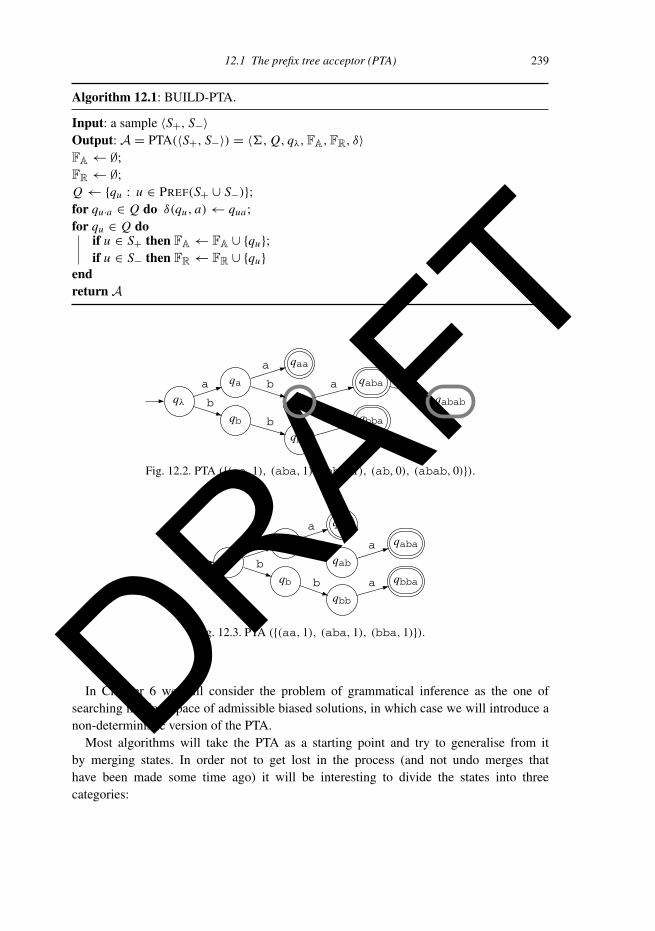
Fig. 12.11. The final filling of the holes for GOLD.

Next, Algorithm GOLD-BUILDAUTOMATON (12.5) is run on the table, with theresulting automaton depicted in Figure 12.11(b). The DFA accepts aa which is in S+,therefore the PTA is returned instead.

One might consider that GOLD-FILLHOLES is far too trivial for such a complex taskas that of learning automata. Indeed, when considering Table 12.5 a certain number of safedecisions about the automaton can be made. These are depicted in Figure 12.11(a). Theothers have to be guessed:

• equivalent lines for a could be λ and b (so qa could be either qλ or qb),• possible candidates for bba are λ and bb (so qbba could be either qλ or qbb),• possible candidates for bbb are λ and bb (so qbbb could be either qλ or qbb).

In the choices above not only should the possibilities before merging be considered, butalso the interactions between the merges. For example, even if in theory both states qa andqbba could be merged into state qλ, they both cannot be merged together! We will not enterhere into how this guessing can be done (greediness is one option).

Therefore the algorithm, having failed, returns the PTA depicted in Figure 12.12(a). If ithad guessed the holes correctly an automaton consistent with the data (see Figure 12.12(b))might have been returned.

12.3.8 Proof of the algorithm

We first want to prove that, alas, filling in the holes is where the real problems start. Thereis no tractable strategy that will allow us to fill the holes easily:

Theorem 12.3.3 (Equivalence of problems) Let RED be a set of states prefix-closed,and S be a sample. Let 〈STA,EXP,OT〉 be an observation table consistent with all thedata in S, with EXP suffix-closed.


qλ

qa

qb

qab

qbb

qabb

qbba

qbbb

a

b

b

b

b

a

b

(a) The PTA.

qλ

qb qbb

b

a

a

b

a,b

(b) The correct solution.

Fig. 12.12. The result and the correct solution.

The question:

Name: ConsistentInstance: A sample S, a prefix-closed set RED

Question: Does there exist a DFA = 〈�, Q, qλ,FA,FR, δ〉 with Q = {qu :u ∈ RED}, and if ua ∈ RED, δ(qu, a) = qua, consistent with S?

is equivalent to:

Name: HolesInstance: An observation table 〈STA,EXP,OT〉Question: Can we fill the holes in such a way as to have 〈STA,EXP,OT〉closed?

Proof If we can fill the holes and obtain a closed table, then a DFA can be constructedwhich is consistent with the data (by Theorem 12.3.1). If there is a DFA with the states ofRED then we can use the DFA to fill the holes.

From this we have:

Theorem 12.3.4 The problem:

Name: Minimum consistent DFA reachable from RED

Instance: A sample S, a set RED prefix-closed such that each OT[s](s ∈ RED) is obviously different from all the others with respect to S, and apositive integer nQuestion: Is there a DFA = 〈�, Q, qλ,FA,FR, δ〉 with the conditions{qu : u ∈ RED} ⊆ Q, |Q| = n, consistent with S?

is NP-complete.

DRAFT12.4 RPNI 255

And as a consequence:

Corollary 12.3.5 Given S and a positive integer n, the question:

Name: Minimum consistent DFAInstance: A sample S and a positive integer nQuestion: Is there a DFA with n states consistent with S?

is NP-complete.

Proof We leave the proofs that these problems are NP-hard to Section 6.2 (page 119).Proving that either of the problems belongs to NP is not difficult: simply producing

a DFA and checking consistency is going to take polynomial time only as it consists ofparsing the strings in S.

On the positive side, identification in the limit can be proved:

Theorem 12.3.6 Algorithm GOLD, given any sample S = 〈S+, S−〉:• outputs a DFA consistent with S,• admits a polynomial-sized characteristic sample,• runs in time and space polynomial in ‖S‖.

Proof• Remember that in the worst case the PTA is returned.• The characteristic sample can be constructed in such a way as to make sure that all the states

are found to be OD. The number of such strings is quadratic in the size of the target automaton.Furthermore it can be proved that none of these strings needs to be of length more than n2. It shouldbe noted that for this to work, the order in which the BLUE states are explored for promotionmatters. If the size of the canonical acceptor of the language is n, then there is a characteristicsample CSL with ‖CSL‖ = 2n2(|�| + 1), such that GOLD(S) produces the canonical acceptorfor all S ⊇ CSL .

• Space complexity is in O(‖S‖·n)whereas time complexity is in O(n2 ·‖S‖). We leave for Exercise12.5 the question of obtaining a faster algorithm.

Corollary 12.3.7 Algorithm GOLD identifies DFA(�) in POLY-CS time.

Identification in the limit in POLY-CS polynomial time follows from the previousremarks.

12.4 RPNI

In Algorithm GOLD, described in Section 12.3, there is more than a real chance that aftermany iterations the final problem of ‘filling the holes’ is not solved at all (and perhapscannot be solved unless more states are added) and the PTA is returned. Even if this ismathematically admissible (since identification in the limit is ensured), in practice one


would prefer an algorithm that does some sort of generalisation in all circumstances, andnot just in the favourable ones.

This is what is proposed by algorithm RPNI (Regular Positive and Negative Inference).The idea is to greedily create clusters of states (by merging) in order to come up with asolution that is always consistent with the learning data. This approach ensures that sometype of generalisation takes place and, in the best of cases (which we can characterise bygiving sufficient conditions that permit identification in the limit), returns the correct targetautomaton.

12.4.1 The algorithm

We describe here a generic version of Algorithm RPNI. A number of variants havebeen published that are not exactly equivalent. These can be studied in due course.Basically, Algorithm RPNI (12.13) starts by building PTA(S+) from the positive data(Algorithm BUILD-PTA (12.1, page 239)), then iteratively chooses possible merges,checks if a given merge is correct and is made between two compatible states (AlgorithmRPNI-COMPATIBLE (12.10)), makes the merge (Algorithm RPNI-MERGE (12.11)) ifadmissible and promotes the state if no merge is possible (Algorithm RPNI-PROMOTE(12.9)).

The algorithm has as a starting point the PTA, which is a deterministic finite automaton.In order to avoid problems with non-determinism, the merge of two states is immediatelyfollowed by a folding operation: the merge in RPNI always occurs between a RED stateand a BLUE state. The BLUE states have the following properties:

• If q is a BLUE state, it has exactly one predecessor, i.e. whenever δ(q1, a1) = δ(q2, a2) = q , thennecessarily q1 = q2 and a1 = a2.

• q is the root of a tree, i.e. if δ(q, u · a)=δ(q, v · b) then necessarily u = v and a = b.

Algorithm 12.9: RPNI-PROMOTE.

Input: a DFA A = 〈�, Q, qλ,FA,FR, δ〉, sets RED,BLUE ⊆ Q, qu ∈ BLUE

Output: A,RED,BLUE updatedRED ← RED ∪ {qu};BLUE ← BLUE ∪ {δ(qu, a), a ∈ �};return A,RED,BLUE

Algorithm RPNI-PROMOTE (12.9), given a BLUE state qu , promotes this state to RED

and all the successors in A of this state become BLUE.Algorithm RPNI-COMPATIBLE (12.10) returns YES if the current automaton cannot

parse any string from S− but returns NO if some counter-example is accepted by the currentautomaton. Note that the automaton A is deterministic.

DRAFT12.4 RPNI 257

Algorithm 12.10: RPNI-COMPATIBLE.

Input: A, S−Output: a Boolean, indicating if A is consistent with S−for w ∈ S− do

if δA(qλ,w) ∩ FA �= ∅ then return falseendreturn true

Algorithm RPNI-MERGE (12.11) takes as arguments a RED state q and a BLUE state q ′.It first finds the unique pair (q f , a) such that q ′ = δA(q f , a). This pair exists and is uniquebecause q ′ is a BLUE state and therefore the root of a tree. RPNI-MERGE then redirectsδ(q f , a) to q. After that, the tree rooted in q ′ (which is therefore disconnected from therest of the DFA) is folded (RPNI-FOLD) into the rest of the DFA. The possible interme-diate situations of non-determinism (see Figure 12.7, page 242) are dealt with during therecursive calls to RPNI-FOLD. This two-step process is shown in Figures 12.13 and 12.14.

Algorithm 12.11: RPNI-MERGE.

Input: a DFA A, states q ∈ RED, q ′ ∈ BLUE

Output: A updatedLet (q f , a) be such that δA(q f , a) = q ′;δA(q f , a)← q;return RPNI-FOLD(A, q, q ′)

Algorithm RPNI (12.13) depends on the choice of the function CHOOSE. Provided it isa deterministic function (such as one that chooses the minimal 〈u, a〉 in the lexicographicorder), convergence is ensured.

The RED states

qλ

q

q f

q ′a

Fig. 12.13. The situation before merging.


Algorithm 12.12: RPNI-FOLD.

Input: a DFA A, states q, q ′ ∈ Q, q ′ being the root of a treeOutput: A updated, where subtree in q ′ is folded into qif q ′ ∈ FA then FA ← FA ∪ {q};for a ∈ � do

if δA(q ′, a) is defined thenif δA(q, a) is defined then

A ←RPNI-FOLD(A, δA(q, a), δA(q ′, a))else

δA(q, a)← δA(q ′, a);end

endendreturn A

The RED states

qλ

q

q f

q ′

a

Fig. 12.14. The situation after merging and before folding.

12.4.2 The algorithm’s proof

Theorem 12.4.1 Algorithm RPNI (12.13) identifies in the limit DFA(�) in POLY-CStime.

Proof We use here Definition 7.3.3 (page 154). We first prove that the algorithm computesa consistent solution in polynomial time. First note that the size of the PTA (‖PTA‖ beingthe number of states) is polynomial in ‖S‖. The function CHOOSE can only be called atmost ‖PTA‖ number of times. At each call, compatibility of the running BLUE state willbe checked with each state in RED. This again is bounded by the number of states in thePTA. And checking compatibility is also polynomial.

Then to prove that there exists a polynomial characteristic set we constructively addthe examples sufficient for identification to take place. Let A = 〈�, Q, qλ,FA,FR, δ〉be the complete minimal canonical automaton for the target language L . Let <CHOOSE

be the order relation associated with function CHOOSE. Then compute the minimum

DRAFT12.4 RPNI 259

Algorithm 12.13: RPNI.

Input: a sample S = 〈S+, S−〉, functions COMPATIBLE, CHOOSEOutput: a DFA A = 〈�, Q, qλ,FA,FR, δ〉A ← BUILD-PTA(S+);RED ← {qλ};BLUE ← {qa : a ∈ � ∩ PREF(S+)};while BLUE �= ∅ do

CHOOSE(qb ∈ BLUE);BLUE ← BLUE \ {qb};if ∃qr ∈ RED such that RPNI-COMPATIBLE(RPNI-MERGE(A, qr , qb), S−) then

A ← RPNI-MERGE(A, qr , qb);BLUE ← BLUE ∪ {δ(q, a) : q ∈ RED ∧ a ∈ � ∧ δ(q, a) �∈ RED};

elseA ← RPNI-PROMOTE(qb,A)

endendfor qr ∈ RED do /* mark rejecting states */

if λ ∈ (L(Aqr )−1S−) then FR ← FR ∪ {qr }

endreturn A

distinguishing string between two states qu, qv (MD), and the shortest prefix of a statequ (SP):

• MD(qu , qv) = min<CHOOSE{w ∈ �� : (δ(qu , w) ∈ FA ∧ δ(qv, w) ∈ FR

) ∨ (δ(qu , w) ∈

FR ∧ δ(qv, w) ∈ FA

)}.• SP(qu) = min<CHOOSE{w ∈ �� : δ(qλ,w) = qu}.RPNI-CONSTRUCTCS(A) (Algorithm 12.14) uses these definitions to build a character-istic sample for RPNI, for the order <CHOOSE, and the target language.

MD(qu, qv) represents the minimum suffix allowing us to establish that states qu andqv should never be merged. For example, if we consider the automaton in Figure 12.15,in which the states are numbered in order to avoid confusion, this string is aa for q1

and q2.SP(qu) is the shortest prefix in the chosen order that leads to state qu . Normally this

string should be u itself. For example, for the automaton represented in Figure 12.15,SP(q1) = λ, SP(q2) = a, SP(q3) = aa and SP(q4) = b.

12.4.3 A run of the algorithm

To run RPNI we first have to select a function CHOOSE. In this case we use the lex-lengthorder over the prefixes leading to a state in the PTA. This allows us to mark the states once


Algorithm 12.14: RPNI-CONSTRUCTCS.

Input: A = 〈�, Q, qλ,FA,FR, δ〉Output: S = 〈S+, S−〉S+ ← ∅;S− ← ∅;for qu ∈ Q do

for qv ∈ Q dofor a ∈ � such that L(Aqv ) ∩ a�� = ∅ and qu �= δ(qv, a) do

w ← MD(qu, qv);if δ(qλ, u · w) ∈ FA then

S+ ← S+ ∪ SP(qu) · w; S− ← S− ∪ SP(qv)a · welse S− ← S− ∪ SP(qu) · w; S+ ← S+ ∪ SP(qv)a · w

endend

endreturn 〈S+, S−〉

q1

q2

q3

q4

a a

b

a

b

b

b

a

Fig. 12.15. Shortest prefixes of a DFA.

and for all. With this order, state q1 corresponds to qλ in the PTA, q2 to qa, q3 to qb ,q4 toqaa, and so forth.

The data for the run are:

S+ = {aaa,aaba,bba,bbaba}S− = {a,bb,aab,aba}

From this we build PTA(S+), depicted in Figure 12.16.We now try to merge states q1 and q2, by using Algorithm RPNI-MERGE with values

A, q1, q2. Once transition δA(q1,a) is redirected to q1, we reach the situation representedin Figure 12.17.

This is the point where Algorithm RPNI-FOLD is called, in order to fold the subtreerooted in q2 into the rest of the automaton; the result is represented in Figure 12.18.

DRAFT12.4 RPNI 261

q1

q2

q3

q4

q5

q6

q7

q8

q9

q10

q11

a

b

a

b

a

b

a

a

b a

Fig. 12.16. PTA(S+).

q1

q2

q3

q4

q5

q6

q7

q8

q9

q10

q11

a

b

a

b

a

b

a

a

b a

Fig. 12.17. After δA(q1,a) = q1.

q1

q3q5

q8

q9

q10

q11

a

b

b

a

a b a

Fig. 12.18. After merging q2 and q1.

q1

q2

q3

q4

q5

q6

q7

q8

q9

q10

q11

a

b

a

b

a

b

a

a

b a

Fig. 12.19. The PTA with q2 promoted.

The resulting automaton can now be tested for compatibility but if we try to parsethe negative examples we notice that counter-example a is accepted. The merge is thusabandoned and we return to the PTA.

State q2 is now promoted to RED, and its successor q4 is BLUE (Figure 12.19).


q1

q2

q3

q4

q5

q6

q7

q8

q9

q10

q11

a

ba

b

a

b

a

a

b a

Fig. 12.20. Trying to merge q3 and q1.

q1

q2

q4

q6

q7

q9

q10 q11

a

ba

a

b a

b

a

Fig. 12.21. After the folding.

q1 q2

q4

q5

q6

q7

q8

q9

q10 q11

a,b

a

b

a

b

a

a

b a

Fig. 12.22. Trying to merge q3 and q2.

So the next BLUE state is q3 and we now try to merge q3 with q1. The automaton inFigure 12.20 is built by considering the transition δA(q1,b) = q1. Then RPNI-FOLD(A,q1, q3) is called.

After folding, we get an automaton (see Figure 12.21) which again parses counter-example a as positive.

Therefore the merge {q1, q3} is abandoned and we must now check the merge betweenq3 and q2. After folding, we are left with the automaton in Figure 12.22 which this timeparses the counter-example aba as positive.

Since q3 cannot be merged with any RED state, there is again a promotion: RED ={q1, q2, q3}, and BLUE = {q4, q5}. The updated PTA is depicted in Figure 12.23.

The next BLUE state is q4 and the merge we try is q4 with q1. But a (which is thedistinguishing suffix) is going to be accepted by the resulting automaton (Figure 12.24).

DRAFT12.4 RPNI 263

q1

q2

q3

q4

q5

q6

q7

q8

q9

q10

q11

a

b

a

b

a

b

a

a

b a

Fig. 12.23. The PTA with q3 promoted.

q1

q2

q3q5

q8

q9

q10

q11

a

bb

a

a

a

b a

Fig. 12.24. Merging q4 with q1 and folding.

q1

q2

q3q5

q6

q8q10

q11

a

ba

b

a

a b a

Fig. 12.25. Automaton after merging q4 with q3.

The merge between q4 and q2 is then tested and fails because of a now being parsed.The next merge (q4 with q3) is accepted. The resulting automaton is shown in Figure 12.25.

The next BLUE state is q5; notice that state q6 has the shortest prefix at that point, butwhat counts is the situation in the original PTA. The next merge to be tested is q5 with q1:it is rejected because of string a which is a counter-example that would be accepted bythe resulting automaton (represented in Figure 12.26). Then the algorithm tries merging q5

with q2: this involves folding in the different states q8, q10 and q11. The merge is accepted,and the automaton depicted in Figure 12.27 is constructed.

Finally, BLUE state q6 is merged with q1. This merge is accepted, resulting in theautomaton represented in Figure 12.28.

Last, the states are marked as final (rejecting). The final accepting ones are correct, butby parsing strings from S−, state q2 is marked as rejecting (Figure 12.29).


q1

q2

q3 q6

q10q11a

b

b

a

b

a

a

Fig. 12.26. Automaton after merging q5 with q1, and folding.

q1

q2

q3

q6a

bab a

Fig. 12.27. Automaton after merging q5 with q2, and folding.

q1

q2

q3

a

b

ab

a

Fig. 12.28. Automaton after merging q6 with q1.

q1

q2

q3

a

b

ab

a

Fig. 12.29. Automaton after marking the final rejecting states.

12.4.4 Some comments about implementation

The RPNI algorithm, if implemented as described above, does not scale up. It needs a lot offurther work done to it before reaching a satisfactory implementation. It will be necessaryto come up with a correct data structure for the PTA and the intermediate automata. Oneshould consider the solutions proposed by the different authors working in the field.

DRAFT12.5 Exercises 265

The presentation we have followed here avoids the heavy non-deterministic formalismsthat can be found in the literature and that add an extra (and mostly unnecessary) difficultyto the implementation.

12.5 Exercises

12.1 Algorithm 12.4 (page 245) has a complexity in O(|STA|2 + |STA| · |E |2). Find analternative algorithm, with a complexity in O(|STA| · |E |).

12.2 Run Gold’s algorithm for the following data:

S+ = {a,abb,bab,babbb}S− = {ab,bb,aab,b,aaaa,babb}

12.3 Take RED = {qλ}, EXP = {λ,b,bbb}. Suppose S+ = {λ,b} and S− = {bbb}.Construct the corresponding DFA, with Algorithm GOLD-BUILDAUTOMATON12.5 (page 247). What is the problem?

12.4 Build an example where RED is not prefix-closed and for which Algorithm GOLD-BUILDAUTOMATON 12.5 (page 247) fails.

12.5 In Algorithm GOLD the complexity seems to depend on revisiting each cell in OTvarious times in order to decide if two lines are obviously different. Propose a datastructure which allows the first phase of the algorithm (the deductive phase) to be inO(n · ‖S‖) where n is the size (number of states) of the target DFA.

12.6 Construct the characteristic sample for the automaton depicted in Figure 12.30(a)with Algorithm RPNI-CONSTRUCTCS (12.14).

12.7 Construct the characteristic sample for the automaton depicted in Figure 12.30(b),as defined in Algorithm RPNI-CONSTRUCTCS (12.14).

12.8 Run Algorithm RPNI for the order relations ≤alpha and ≤lex-length on

S+ = {a,abb,bab,babbb}S− = {ab,bb,aab,b,aaaa,babb}.

12.9 We consider the following definition in which a learning algorithm is supposed tolearn from its previous hypothesis and the new example:

q1

q2

q3

a

b

b

a

ab

(a)

q1

q2

q3

a

a

b

a

b

b

(b)

Fig. 12.30. Target automata for the exercises.


Definition 12.5.1 An algorithm A incrementally identifies grammar class G inthe limit ifdef given any T in G, and any presentation φ of L(T ), there is a rank nsuch that if i ≥ n, A(φ(i),Gi ) ≡ T .

Can we say that RPNI is incremental? Can we make it incremental?12.10 What do you think of the following conjecture?

Conjecture of non-incrementality of the regular languages. There exists noincremental algorithm that identifies the regular languages in the limit from aninformant. More precisely, let A be an algorithm that given a DFA Ak , a currenthypothesis, and a labelled string wk (hence a pair 〈wk, l(wk)〉), returns an automa-ton Ak+1. In that case we say that A identifies in the limit an automaton T ifdef forno rank k above n, Ak �≡ T .

Note that l(w) is the label of string w, i.e. 1 or 0.12.11 Devise a collusive algorithm to identify DFAs from an informant. The algorithm

should rely on an encoding of DFAs over the intended alphabet �. The algorithmchecks the data, and, if some string corresponds to the encoding of a DFA, thisDFA is built and the sample is reconsidered: is the DFA minimal and compatible forthis sample? If so, the DFA is returned. If not, the PTA is returned. Check that thisalgorithm identifies DFAs in POLY-CS time.

12.6 Conclusions of the chapter and further reading

12.6.1 Bibliographical background

In Section 12.1 we have tried to define in a uniform way the problem of learning DFAsfrom an informant. The notions developed here are based on the common notion of theprefix tree acceptor, sometimes called the augmented PTA, which has been introduced byvarious authors (Alquézar & Sanfeliu, 1994, Coste & Fredouille, 2003). It is customary topresent learning in a more asymmetric way as generalising from the PTA and controllingthe generalisation (i.e. avoiding over-generalisation) through the negative examples. Thisapproach is certainly justified by the capacity to define the search space neatly (Dupont,Miclet & Vidal, 1994): we will return to it in Chapters 6 and 14.

Here the presentation consists of viewing the problem as a classification question andgiving no advantage to one class over another. Among the number of reasons for preferringthis idea, there is a strong case for manipulating three types of states, some of which are ofunknown label. There is a point to be made here: if in ideal conditions, and when conver-gence is reached, the hypothesis DFA (being exactly the target) will only have final states(some accepting and some rejecting), this will not be the case when the result is incorrect.In that case deciding that all the non-accepting states are rejecting is bound to be worsethan leaving the question unsettled.

The problem of identifying DFAs from an informant has attracted a lot of attention:E. Mark Gold (Gold, 1978) and Dana Angluin (Angluin, 1978) proved the intractability of

DRAFT12.6 Conclusions of the chapter and further reading 267

finding the smallest consistent automaton. Lenny Pitt and Manfred Warmuth extended thisresult to non-approximability (Pitt & Warmuth, 1993). Colin de la Higuera (de la Higuera,1997) noticed that the notion of polynomial samples was non-trivial.

E. Mark Gold’s algorithm (GOLD) (Gold, 1978) was the first grammatical inferencealgorithm with strong convergence properties. Because of its incapacity to do better thanreturn the PTA the algorithm is seldom used in practice. There is nevertheless room forimprovement. Indeed, the first phase of the algorithm (the deductive step) can be imple-mented with a time complexity of O(‖S‖ · n) and can be used as a starting point forheuristics.

Algorithm RPNI is described in Section 12.4. It was developed by Jose Oncina andPedro García (Oncina & García, 1992). Essentially this presentation respects the originalalgorithm. We have only updated the notations and somehow tried to use a terminologycommon to the other grammatical inference algorithms. There have been other alter-native approaches based on similar ideas: work by Boris Trakhtenbrot and Ya Barzdin(Trakhtenbrot & Bardzin, 1973) and by Kevin Lang (Lang, 1992) can be checked fordetails.

A more important difference in this presentation is that we have tried to avoid the non-deterministic steps altogether. By replacing the symmetrical merging operation, whichrequires determinisation (through a cascade of merges), by the simpler asymmetric foldingoperation, NFAs are avoided.

In the same line, an algorithm that doesn’t construct the PTA explicitly is presented in(de la Higuera, Oncina & Vidal, 1996). The RED, BLUE terminology was introduced in(Lang, Pearlmutter & Price, 1998), even if does not coincide exactly with previous defini-tions: in the original RPNI the authors use shortest prefixes to indicate the RED states andelements of the kernel for some prefixes leading to the BLUE states. Another analysis ofmerging can be found in (Lambeau, Damas & Dupont, 2008).

Algorithm RPNI has been successfully adapted to tree automata (García & Oncina,1993), and infinitary languages (de la Higuera & Janodet, 2004).

An essential reference for those wishing to write their own algorithms for this task isthe datasets. Links about these can be found on the grammatical inference webpage (vanZaanen, 2003). One alternative is to generate one’s own targets and samples. This can bedone with the GOWACHIN machine (Lang, Pearlmutter & Coste, 1998).

12.6.2 Some alternative lines of research

Both GOLD and RPNI have been considered as good starting points for other algorithms.During the ABBADINGO competition, state merging was revisited, the order relationbeing built during the run of the algorithm. This led to heuristic EDSM (evidence drivenstate merging), which is described in Section 14.5.

More generally the problem of learning DFAs from positive and negative strings hasbeen tackled by a number of other techniques (some of which are presented in Chapter 14).


12.6.3 Open problems and possible new lines of research

There are a number of questions that still deserve to be looked into concerning the problemof learning DFAs from an informant, and the algorithms GOLD and RPNI:

Concerning the problem of learning DFAs from an informant. Both algorithms wehave proposed are incapable of adapting correctly to an incremental setting. Even if a firsttry was made by Pierre Dupont (Dupont, 1996), there is room for improvement. Moreover,one aspect of incremental learning is that we should be able to forget some of the data weare learning from during the process. This is clearly not the case with the algorithms wehave seen in this chapter.

Concerning the GOLD algorithm. There are two research directions one could recom-mend here. The first corresponds to the deductive phase. As mentioned in Exercise 12.5,clever data structures should accelerate the construction of the table with as manyobviously different rows as possible.

The second line of research corresponds to finding better techniques and heuristics to fillthe holes.

Concerning the RPNI algorithm. The complexity of the RPNI algorithm remains looselystudied. The actual computation which is proposed is not convincing, and empirically,those that have consistently used the algorithm certainly do not report a cubic behaviour. Abetter analysis of the complexity (joined with probably better data structures) is of interestin that it would allow us to capture the parts where most computational effort is spent.

Other related topics. A tricky open question concerns the collusion issues. An alternative‘learning’ algorithm could be to find in the sample a string which would be the encodingof a DFA, decode this string and check if the characteristic sample for this automaton isincluded. This algorithm would then rely on collusion: it needs a teacher to encode theautomaton. Collusion is discussed in (Goldman & Mathias, 1996): for the learner-teachermodel to be able to resist collusion, an adversary is introduced. This, here, corresponds tothe fact that the characteristic sample is to be included in the learning sample for identifica-tion to be mandatory. But the fact that one can encode the target into a unique string, whichis then correctly labelled and passed to the learner together with a proof that the numberof states is at least n, which has been remarked in a number of papers (Castro & Guijarro,2000, Denis & Gilleron, 1997, Denis, d’Halluin & Gilleron, 1996) remains troubling.

Documents

12 - Université de Nantes