Embed Size (px)
Citation preview
(12) United States Patent Krishnamurthy et al.
USOO881.2487B2
US 8,812,487 B2 Aug. 19, 2014
(10) Patent No.: (45) Date of Patent:
(54)
(75)
(73)
(*)
(21)
(22)
(65)
(60)
(51)
(52)
(58)
ADDITION AND PROCESSING OF CONTINUOUS SQL QUERIES INA STREAMING RELATIONAL DATABASE MANAGEMENT SYSTEM
Inventors: Saileshwar Krishnamurthy, Palo Alto, CA (US); Neil Thombre, Santa Clara, CA (US); Neil Conway, Berkeley, CA (US); Wing Hang Li, San Bruno, CA (US); Morten Hoyer, Montclair, NJ (US)
Assignee: Cisco Technology, Inc., San Jose, CA (US)
Notice: Subject to any disclaimer, the term of this patent is extended or adjusted under 35 U.S.C. 154(b) by 306 days.
Appl. No.: 12/398.944
Filed: Mar. 5, 2009
Prior Publication Data
US 2009/0228434 A1 Sep. 10, 2009
Related U.S. Application Data Provisional application No. 61/068,572, filed on Mar. 6, 2008.
Int. C. G06F 7700 (2006.01) G06F 7/30 (2006.01) U.S. C. CPC. G06F 17/30516 (2013.01); G06F 17/30445
(2013.01); G60F 17/30545 (2013.01) USPC .......................................................... T07/718 Field of Classification Search CPC .................... G06F 17/30516; G06F 17/30424;
GO6F 17/30929 USPC .......................................................... 707/718 See application file for complete search history.
(56) References Cited
U.S. PATENT DOCUMENTS
2009/0106198 A1* 4/2009 Srinivasan et al. ................ 707/3 2009/0106214 A1* 4/2009 Jain et al. .......................... 7O7/4 2009/02284.65 A1 9/2009 Krishnamurthy et al. 2011/0302164 Al 12/2011 Krishnamurthy et al.
OTHER PUBLICATIONS
"Shared Query Processing in Data Streaming Systems” by Saileshwar Krishnamurthy, Fall 2006.* Saileshwar Krishnamurthy, "Shared Query Processing in Data Streaming Systems.” University of California, Berkeley, 2006, pp. 1-212.
(Continued)
Primary Examiner — Jacob F Bétit Assistant Examiner — Christy Lin (74) Attorney, Agent, or Firm — Hickman Palermo Truong Becker Bingham Wong LLP
(57) Systems, methods, and media are disclosed herein that can be embodied in a traditional Relational Database Management System (RDBMS) in order to transform it into a Streaming Relational Database Management System (SRDBMS). An SRDBMS may provide functionality such as to manage and populate streams, tables, and archived stream histories and Support the evaluation of continuous queries on streams and tables. Both continuous and Snapshot queries Support the full spectrum of the industry standard, widely used, Structured Query Language. The present technology can Support a high number of concurrent continuous queries using a scalable and efficient shared query evaluation scheme, Support on-the-fly addition of continuous queries into a mechanism that imple ments the shared evaluation scheme, reuse RDBMS modules Such as relational operators and expression evaluators, and visualize results of continuous queries in real time.
ABSTRACT
8 Claims, 4 Drawing Sheets
- N 200
Runtime Module plar
Folding Module 232
230 Tuple Router 234.

US 8,812.487 B2 Page 2
(56) References Cited
OTHER PUBLICATIONS
Altinel, Mehmet etal. "Cache Tables: Paving the Way for an Adaptive Database Cache.” Proceedings of the 29th VLDB Conference, Berlin, Germany, 2003. Franklin, Michael J. et al. “Design Considerations for High Fan-in Systems: the HiFi Approach.” Proceedings of the 2nd CIDR Confer ence, Asilomar, California, 2005. Krishnamurthy, Sailesh et al. "On-the-Fly Sharing for Streamed Aggregation.” SIGMOD Conference 2006, Chicago, Illinois, Jun. 27-29, 2006. Krishnamurthy, Sailesh et al. “The Case for Precision Sharing.” Pro ceedings of the 30th VLDB Conference, Toronto, Canada, 2004. Krishnamurthy, Sailesh et al. “Shared Hierarachical Aggregation for Monitoring Distributed Streams.” Report No. UCB/CSD-05-1381. Computer Science Division, University of California, Berkeley, Oct. 18, 2005. Chandrasekaran, Sirish et al. “TelegraphCQ: Continuous Dataflow Processing for an Uncertain World.” Proceedings of the 1st CIDR Conference, Asilomar, California, 2003.
Krishnamurthy, Sailesh etal. “Telegraph CQ: An Architectural Status Report.” Bulletin of the IEEE Computer Society Technical Commit tee on Data Engineering, Nov. 18, 2003. Krishnamurthy, Saileshwar. “Shared Query Processing in Data Streaming Systems.” A dissertating Submitted in partial satisfaction of the requirements for the degree of Doctor of Philoshophy in Computer Science in the graduate division of the University of Cali fornia, Berkeley. Fall 2006. "Shared Query Processing in Data Streaming Systems', by Saileshwar Krishnamurthy, Fall 2006, http://citeseerx.ist.psu.edu/ viewdoc/download? Doi=10.1.1. 122, 1989&rep1&type=pdf. T. Johnson et al., “A Heartbeat Mechanism and its Application in Gigascope'. Proceedings of the 31 VLDB Conference, Norway 2005, pp. 1079-1088. Nalamwar, A., “Blocking Operators and Punctuated Data Streams in Continuous Query Systems' Compter Science, Feb. 1, 2003, pp. 1-19. Tucker, Peter A. et al., “Exploiting Punctuation Semantics in Con tinuous Data Streams”, IEEE Transactions on Knowledge and Data Engineering, May/Jun. 2003, pp. 555-568.
* cited by examiner

US 8,812.487 B2 Sheet 1 of 4 Aug. 19, 2014 U.S. Patent
| eun61–
?ssepold Å?enb snonu?uoo • Lueens eleC ,
bussooid kºnb ºpou ?pieg • uueens elepandul „eilua, e uene? Auenb "sug euous •
US 8,812.487 B2 U.S. Patent

U.S. Patent Aug. 19, 2014 Sheet 3 of 4 US 8,812.487 B2
Eiff grass: First
elapse 8888 pšrisixar &xseisskie
to press Sists of


US 8,812,487 B2 1.
ADDITION AND PROCESSING OF CONTINUOUS SQL QUERIES INA
STREAMING RELATIONAL DATABASE MANAGEMENT SYSTEM
CROSS-REFERENCE TO RELATED APPLICATIONS
This application claims the priority benefit of U.S. Provi sional Patent Application No. 61/068,572 filed on Mar. 6, 2008, titled "On-the-Fly Addition, Shared Evaluation, and Declarative Visualization of Continuous SQL Queries in a Streaming Relational Database Management System.” which is incorporated herein by reference. The present application is with U.S. patent application Ser. No. 12/398.959 filedon Mar. 5, 2009, titled “Systems and Methods for Managing Queries.” which also claims priority to U.S. Provisional Patent Appli cation No. 61/068,572.
FIELD OF THE APPLICATION
The present application relates to database management.
SUMMARY
Various embodiments of the invention disclose techniques that can be embodied in a traditional RDBMS (Relational Database Management System) in order to transform it into an SRDBMS (Streaming Relational Database Management System). Such a transformed SRDBMS may provide at least the following functionality:
1. Manage and populate streams, tables, and archived stream histories.
2. Support the evaluation of continuous queries on streams and tables.
3. Both continuous and Snapshot queries Support the full spectrum of the industry standard, widely used, Struc tured Query Language (SQL).
Various embodiments of the invention provide: 1. Support for a very high number of concurrent continuous
queries using a highly scalable and efficient shared query evaluation scheme.
2. Support for on-the-fly addition of continuous queries into the mechanism that implements the shared evalua tion scheme.
3. To reuse existing modules of the RDBMS such as rela tional operators and expression evaluators as much as possible.
4. To visualize the results of continuous queries in real time
BRIEF DESCRIPTION OF THE DRAWINGS
FIG. 1 is a block diagram illustrating a database centric environment and a database stream environment.
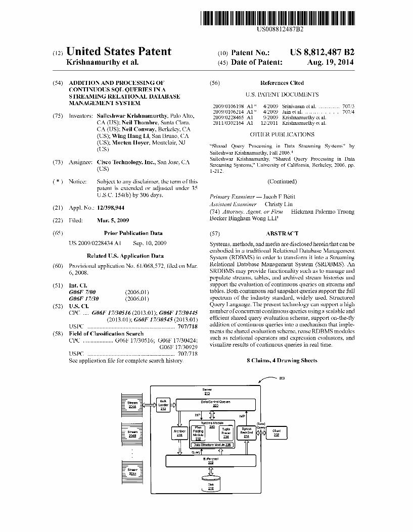
FIG. 2 is a block diagram illustrating an embodiment of a streaming relational database management system.
FIG. 3 is a block diagram illustrating an embodiment of a streaming relational database management system.
FIG. 4 illustrates a prompt for entering query parameters in a streaming relational database management system.
DETAILED DESCRIPTION
A Relational Database Management System (RDBMS) is used to store and manipulate finite sets of structured data. At a bare minimum, an RDBMS provides facilities to create and populate database objects such as tables, modify the contents
10
15
25
30
35
40
45
50
55
60
65
2 of these objects, and evaluate SQL queries that process one or more tables in order to produce a relation as an output. More over, a traditional database uses a paradigm called “store first, query later where new data is stored in the database before it can be queried. In effect, these systems manage data that is “at rest' where a query operates on a Snapshot of the database at any point in time—Such a query is called 'snapshot queries' (SQ). An SQ runs in a finite amount of time and produces a single set of records every time it is invoked.
FIG. 1 illustrates the contrasts between database-centric approaches versus datastream-centric approaches. Streams of data may include data that is “on the move' in addition to data that is at rest. Systems that manage streams of data are called Streaming Relational Database Management Systems (SRDBMS) and are disclosed herein. A query that is deployed over one or more stream in an SRDBMS runs forever and is called a “continuous query” (CQ). As a new datum enters the system it is processed in order to produce additional results for the queries. Logically, a stream of data can be thought of as an unbounded set of tuples (i.e., records), ordered by a designated timestamp attribute called the CQTIME attribute. A stream appears in a CO with an associated 'stream-to relation” (StoR) or window clause that expresses how to generate an ordered sequence of finite relations from an unbounded stream. The semantics of a CO is to apply its associated SQ (formed by eliding all StoR clauses in the CQ) in turn on each Such finite relation in the generated sequence, and concatenating the resulting relations into an output Stream.
A stream query processor such as an SRDBMS is primarily used for monitoring and alerting applications. However, an SRDBMS is more than avanilla stream query processor since it integrates the world of streams with those of relations. Thus, in addition to monitoring applications, an SRDBMS can be used to dramatically speed up the performance of traditional analytical and reporting database systems. This performance boost is achieved by exploiting the fact that all data originates as part of some stream (e.g., application, trans action, logs) and can be pre-processed in incremental fashion using CQ technology.
Various embodiments of the invention can be realized using several techniques that are added to a traditional RDBMS along with the development of a client-server inter net infrastructure. We first describe the general architecture of such a system (a Streaming RDBMS) and then embodiments of the invention. Note that, while this document refers to the names of certain data structures and components from the PostgreSQL RDBMS for ease of exposition, the techniques that comprise the embodiments of the invention can be imple mented in any traditional RDBMS.
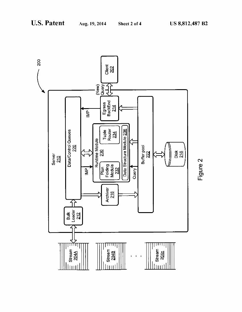
FIG. 2 illustrates an exemplary environment in which embodiments of the present invention may be practiced. FIG. 2 illustrates a block diagram of an embodiment of a streaming relational database management system (SRDBMS) 200 in accordance with aspects of the technology. As with all other figures provided herein, FIG. 2 is exemplary only. The system 200 includes a client 202 in communication with a server 210. For simplicity and clarity, only one client 202 is illustrated in FIG. 2. However, a person having ordinary skill in the art will appreciate that multiple clients 202 may communicate with the server 210.
In some embodiments, the server 210 may include a bulk loader 212, an egress backend 214, an optional archiver 216, a disk 218, data/control queues 220, a buffer pool 222, and a runtime module 230. The egress backend 214 may include a planner, a parser, an optimizer, an executor, and/or the like (not illustrated). The buffer pool 222 may be a disk cache. The

US 8,812,487 B2 3
runtime module 230 includes a plan folding module 232, a tuple router 234, and a data structure module 236. Further details of these elements are provided later herein. The bulk loader 212 is configured to receive tuples from
one or more stream 204A. . .204n. In some embodiments, the bulk loader 212 receives tuples from a client application (not shown) configured to process streams of data (e.g., stream 204A-204n) and provide the tuples to the bulkloader 212. For simplicity and clarity, only one bulk loader 212 is illustrated in FIG. 2. However, a person having ordinary skill in the art will appreciate that the server 210 may include multiple bulk loaders 212 in communication with multiple streams 204A. . . 204n. In some embodiments, the streams 204A. . . 204n communicate the tuples to the server 210 via a network (not shown). The network may be a local area network, a wide area network, a wireless network, a mobile network, the Inter net, the worldwide web, a client and/or the like. Vastarrays of information may be accessible via data sources coupled to networks other than Streams 204A. . . 204n. For example, data can be Supplied by one or more data sources within a local area network, a wide area network, and/or a mobile network. The bulkloader 212 may provide the tuples received from the streams 204A. . . 204n to the data/control queues 220.
In some embodiments, the bulk loader 212 and the egress backend 214 comprise common code configured to receive data including queries and/or tuples from a client application. The common code may be referred to as a bulk loader 212 when receiving tuples. The common code may be referred to as an egress backend 214 when receiving a query. The data/control queues 220 may be configured to receive
tuples from the bulk loader 212 and/or the runtime module 230. The data/control queues 220 may provide the received tuples to the archiver 216, the runtime module 230, and/or the egress backend 214. For example, data/control queues 220 may provide the tuples received from the bulk loader 212 and/or the runtime module 230 to the archiver 216 for storage on the disk 218. The data/control queues 220 may also retrieve the tuples from the bulk loader 212 and provide them to the runtime module 230 for processing.
In some embodiments, the data/control queues 220 and the buffer pool 222 both occupy shared memory. However, they may serve different functions. For example, the buffer pool 222 may function as a disk cache configured to store and retrieve data from tables (e.g., on the disk 218). Thus, the archiver 216 may write data to the disk 218 via the buffer pool 222. However, the buffer pool 222 may be separate and dis tinct from the data/control queues 220.
The disk 218 may be a computer readable medium config ured to store data. Computer readable storage media may include a hard disk, random access memory, read only memory, an optical disk, a magnetic disk, Virtual memory, a network disk, and/or the like. Data may include tuples, tables, variables, constants, queries, continuous queries, programs, IMPs, SCPs, and/or the like. The disk 218 may also store instructions for execution by a processor (not shown), which causes the processor to manage a query. In various embodi ments, instructions for execution on the processor include instructions for implementing the bulk loader 212, the egress backend 214, the archiver 216, the data/control queues 220, the buffer pool 222, and/or the runtime module 230 (including the plan folding module 232, the tuple router 234, and the data structure module 236). The egress backend 214 may receive a query from the
client 202. In various embodiments, the query is a CO or a static query. Optionally, the query received from the client 202 is a new query. The egress backend 214 is configured to
10
15
25
30
35
40
45
50
55
60
65
4 process the new query using a planner, a parser, an optimizer and/or an executor. In some embodiments, the egress backend 214 provides an IMP to the data/control queues 220. The data/control queues 220 may provide the IMP to the runtime module 230. The plan folding module 232 of runtime module 230 is configured to fold the received IMP into a SCP in the data structure module 236. Alternatively, the data/control queues 220 may store the IMP on the disk 218 (e.g., via the archiver 216 and the buffer pool 222) for later use.
In some embodiments, the data/control queues 220 receives database objects (such as streams, tables, relations, views, and/or the like) and provides the database objects to the buffer pool 222 via the archiver 216. The buffer pool 222 may store the database objects on the disk 218. The data/ control queues 220 may provide the database objects to the runtime module 230. Optionally, the data/control queues 220 provide multiple objects to the runtime module 230 at the same time. For example, the data/control queues 220 may provide tuples from two or more streams 204A. . . 204n and a table to a SCP in the data structure module 236 of the runtime module 230. The runtime module 230 is configured to receive tuples
and/or tables from the data/control queues 220. The runtime module 230 may evaluate the tuples and/or tables using the tuple router 234 and the data structures in the data structure module 236. In various embodiments, the runtime module 230 outputs streams, tables, and/or data to the data/control queues 220. The data/control queues 220 may communicate output from the runtime module 230 to the client 202 via the egress backend 214. For example, the data/control queues 220 may receive a tuple from the runtime module 230 and provide the tuple to the archiver 216. The archiver 216 may provide the tuple to the buffer pool 222. The buffer pool 222 may provide the tuple to the egress backend 214. The egress backend 214 may provide the tuple to the client 202. Alter natively, the buffer pool 222 may provide the tuple to the disk 218. Thus, the data/control queues 220 may store output from the runtime module 230 onto the disk 218 via the archiver 216 and the buffer pool 222.
Various kinds of objects (e.g., tables or views) behave like relations in a traditional RDBMS. Objects that behave like streams may be used in the SRDBMS200. In various embodi ments, a stream (e.g., the streams 204A. . . 204n) is classified as a raw stream or derived stream. The classification may be based on how the stream is populated. A raw stream may be populated by an external data provider. In some embodi ments, the external data provider connects to the server 210 using a secure and well-defined protocol that authenticates itself, and advertises the identity of the stream being popu lated. If authorized, the provider may provide data tuples that are appended to the stream. In practice, a data provider will use a call-level API that the SRDBMS provides. A produced stream may be defined using a query (e.g., a
defining query) and may be populated by the SRDBMS 200. A produced stream may be one of multiple types of database objects, including a view and a derived stream. A view may be a database object that is defined using a query and has macro semantics. A view may be defined using a CO as a streaming view. A view may be used in another query in a place that a raw stream can be used. A defining query of a view runs only when a query that uses the view runs as well.
In some embodiments, a derived stream is a materialized CQ that may be associated with a stream using a special syntax (e.g., CREATE STREAM. . . AS query). The associ ated stream is similar to a view and may be used in another query in a place that a raw stream can be used. Unlike a view, however, a derived stream does not have macro Semantics. A

US 8,812,487 B2 5
derived stream may be active, whether or not it is used in another active query. A raw stream and/or a derived stream may be stored on the disk 218, as discussed elsewhere herein. For example, a raw stream and/or a derived stream may be archived using the archiver 216 for storing on the disk 218.
In some embodiments, the runtime module 230 receives a query from the disk 218 via the buffer pool 222. The runtime module 230 may also receive various kinds of objects (e.g., a stream, a data table, metadata, tuples, views, relations, expressions, and/or the like) from the buffer pool 222. These objects may be received by the buffer pool 222 from the disk 218 and/or the archiver 216.
FIG. 3 illustrates the architecture of an SRDBMS that is built using such an RDBMS as a substrate. The following embodiments are exemplary and are meant to be illustrative of the disclosure herein. The examples are not intended to be interpreted as limiting the scope of the present disclosure.
In a traditional process-oriented RDBMS, there is gener ally a process that listens on to incoming connections on a specified socket (the Listener) and forks off a separate “back end process' to handle a new connection. In addition to the Listener, there may be a process dedicated to shared evalua tion of CQs (the Runtime) as well as process dedicated to archiving the results of CQs (the Archiver) in tables. The Archiver process is used to materialize the results of a CO into a persistent RDBMS object such as a traditional table, called an active table. Ingress and Egress of data may be accom plished using standard backend processes and protocols. More specifically, a client producing data for a stream can connect to a backend and use the standard bulk loader for tables (a protocol called COPY) to push data into a stream the backend process takes the incoming records and writes them onto data queues. A client that needs to consume data from the system can connect to a backend and issue a CO using a cursor (in a manner identical to an SQ) and continu ously fetch the results of the CQ by manipulating the cursor. When a backend process receives a query it uses an opti
mizer to produce an execution plan that comprises a tree of relational operators conforming to the well-known “iterator model. If the query in question is an SQ, the backend evalu ates the execution plan individually using its executor com ponent, as would the case be in a traditional RDBMS. If, on the other hand, the query is a CO the backend sends the associated execution plan to the Runtime for shared evalua tion using a control queue. In the latter case, for example, the backend actually evaluates a small 'stub execution plan that consists solely of a Scan operator that reads records from an internal queue in response to FETCH requests from a cursor. When the Runtime process fetches a new query plan, it
merges the new query plan on-the-fly onto a novel shared query plan—this process is called “plan folding.” The shared query plan comprises a set of special CQ operators and an associated “routing table. Apart from plan folding, a respon sibility of the Runtime is to process incoming data records that are fetched from data queues. The runtime accomplishes this by adaptively routing tuples through the CQ operators that constitute the shared plan. These CQ operators perform their associated tasks by reusing the existing implementation of iterator-style relational operators in the RDBMS. In other words, these CQ operators maintain the information associ ated with sharing multiple concurrent queries by "orchestrat ing an arbitrary portion of a standard query plan. Some of these CQ operators, have the added responsibility of writing their results to data queues, from where the tuples are further processed by either an egress backend or the Archiver pro CCSS,
10
15
25
30
35
40
45
50
55
60
65
6 A stream can be thought of as an unbounded, potentially
infinite, bag of tuples, where each tuple has a clearly delin eated “timestamp' attribute. In practice, a stream is a database object that is defined with a schema similar to that of a relation, and tuples are appended to a stream as they “arrive' in the system. The schema of a stream is distinguished from that of a
relation by the following requirements: 1. The designated “timestamp' attribute of a stream is
identified using a COTIME constraint with syntax that is similar to that of NOT NULL and UNIQUE constraints while defining tables.
2. Every stream has one, and only one, attribute with a CQTIME constraint, and this attribute has an ordinal type that is one of SMALLINT, INTEGER, BIGINT, TIMESTAMP, or TIMESTAMPTZ.
3. The values of the CQTIME attribute are monotonically increasing for newer tuples that arrive in the stream.
In the SRDBMS, there can be different kinds of database objects that behave like streams, just as there can be different kinds of objects that behave like relations (e.g., tables, views) in a traditional RDBMS. Thus, streams can be classified as being, for example, raw streams, or derived streams, based on how they are populated:
1. Raw streams. A raw stream is populated by an external data provider that connects to the system using a secure and well-defined protocol that authenticates itself, and advertises the identity of the stream being populated. If authorized, the provider then proceeds to pump in data tuples that are appended to the stream. In practice, a data provider will use a call-level API that the SRDBMS provides.
2. Produced streams. A produced stream is sometimes defined using a query (the "defining query’) and is popu lated by the SRDBMS. A produced stream can be one of the following types of database objects: a. View. A view that is defined with a continuous query is
a streaming view, and can be used in another query in any place that a raw stream can be used. The defining query of a view runs when a query that uses the view is actually running. This is because a view is a data base object that is defined with a query and has "macro' Semantics. A use of a view in another query is identical to explicitly exploding the view’s defining query as a sub-query.
b. Derived streams. A materialized continuous query is explicitly associated with a stream using a special syntax: CREATE STREAM. . . AS query. The asso ciated stream is similar to a view and may be used in another query in any place that a raw stream can be used. Unlike a view, however, a materialized query does not have macro semantics, and is sometimes active whether or not it is used in another active query.
A raw or derived stream can optionally be archived. In order to provide context for the details of the embodi
ments of the invention disclosed herein, a brief description of the syntax and semantics of SQL-based continuous queries is provided. A continuous query (CQ) operates over a set of streams and relations, and produces a stream as output. In order to understand the execution model of a CO a CO is distinguished from a Snapshot query (SQ) in at least the following ways:
1. The FROM clause of a CO has at least one stream. 2. Streams may not appear anywhere else (e.g. WHERE
clause) in a CO. 3. A stream in the FROM clause of a CO may be a stream,
a Derived streams, a view, or an inline Sub-query. Fur
US 8,812,487 B2 7
thermore, a streaming sub-query may be executed as an independent “inner CQ that produces streaming results that can be used to process the “outer CQ.
4. A stream in the FROM clause of a CQ can be optionally associated with a Stream-to-Relation (StoR) operator (informally called a “window” clause). The StoR opera tor describes both the content of a visible set, as well as how the visible set changes over time (e.g., advance by row, advance by time). A visible set of a stream can be thought of as a temporary relation and is valid until it is redefined by the next visible set produced for the same Stream.
5. While there can be more than one stream in the same FROM clause of a given CQ, in order to express a stream-stream join, or a self-join involving streams, all but one of these streams may be defined with a special StoR called a "current window. The "current window' of a stream treats the latest window produced by it as a finite set of records.
6. The SELECT clause of a CQ can optionally be associ ated with a Relation-to-Stream (RtoS) operator that is defined using syntax similar to a DISTINCT clause. An RtoS operator takes a sequence of relations as input and produces a sequence of relations as output.
7. The Relation-to-Relation (RtoR) operator corresponds to the underlying SQ that can be produced by stripping the CQ of its StoR and RtoS clauses.
The SRDBMS offers the capability to execute continuous queries over streams and relations in the standard, and well understood, SQL query language.
The execution of a CO can be easily and unambiguously understood in terms of its StoR operators, its RtoS operator, and its RtoR operator as follows:
1. Apply StoR operators: Every StoR operator (informally called a “window) is continually applied to each asso ciated stream in order to produce an unbounded sequence of visible sets.
2. Apply RtoR operator: Every time a new visible set is produced by an StoR operator, the RtoR operator (i.e., the underlying SQ) is applied on the visible sets and other relations in the FROM clause in order to produce an unbounded sequence of relations.
3. Relation-to-Stream (RtoS) operator: Every time a new relation is produced by applying the RtoR operator, it is used to produce a new “window” of tuples, generally by comparing the relation freshly produced by the RtoR operator with previous relations produced by the RtoR operator. The RtoS operator in the SRDBMS may be used to append successive windows of tuples in order to form a stream.
Stream-to-Relation (StoR) Operators The SRDBMS offers a wide range of StoR operators in
order to satisfy a variety of use cases. Most of these variants are specified in terms of “intervals” that describe contiguous subsequences of the underlying stream. These intervals can be specified in three different kinds of units:
1. Row-based: This interval contains a fixed number of rows in the associated stream. The interval is sometimes specified as an integer: for example, 25 ROWS.
2. Time-based: This interval contains all the rows that fall into a fixed range of time in the associated stream. The data type of this interval depends on the CQTIME type used by the associated stream. For example, when the CQTIME of the stream is a TIMESTAMP, a time-based interval is specified as an INTERVAL value.
3. Window-based: This interval can only be used with a produced stream. It contains all the rows in a fixed num
10
15
25
30
35
40
45
50
55
60
65
8 ber of windows in the underlying stream. It therefore provides a level of abstraction, allowing the properties of a higher-level query to be specified in terms of the StoR used by a lower-level query.
More specifically, the SRDBMS supports the following varieties of StoR operators (the details and the formal syntax are explained herein):
1. Sliding windows: A sliding window is expressed using an advance interval, and a visible interval. The former defines the periodic intervals (and thus, the actual edges) at which a new visible set is constructed from the stream, while the latter defines the interval of tuples, relative to the periodic edges, that belong in each visible set. Note that both intervals can be either time or row based inter vals. When the visible interval exceeds the advance interval, successive visible sets can be thought of as being “sliding” or “moving windows, and a tuple in a stream can thus belong to multiple visible sets.
2. Chunking windows: A chunking window is expressed using either a SAME TIME clause, or a sequence of intervals of the same type (e.g., 2 seconds, 3 seconds, 2 seconds). In the former case, a new visible set is defined every time there is a new tuple in the stream with a timestamp (CQTIME attribute) that is different from the previous tuple. That is, each visible set comprises all tuples with identical timestamps. In the latter case, vis ible sets correspond to sets of tuples whose sizes are defined by the sequence of intervals that is used to express the window, and these visible sets continuously cycle through the sequence of intervals with a period equal to the sum of the intervals in the sequence. Note that in both cases, the underlying stream is broken into successive, contiguous, and non-overlapping "chunks' of tuples." Such non-overlapping windows are often efficient to implement as they generally require no buffering of input data.
3. Landmark windows: A landmark window is expressed using an advance interval, and a reset interval. The former defines the periodic interval (and thus, the actual “advance edges') at which a new visible set is con structed from the stream, while the latter defines a peri odic interval that is used to compute a sequence of “reset' edges. Each visible set comprises all tuples that have arrived in the stream after the latest reset edge. The landmark window is unbounded, and can be visualized as a “rubber-band interval with a fixed left edge, and a right edge that keeps stretching at every advance point. and a left edge that catches up (snaps) with the right edge at every reset point. Note that both the advance and reset intervals can be either time or row based.
The SELECT Command The enhancements (shown in bold) made to the SELECT
statement of ISO standard SQL in order to support streams are described in the following syntax diagrams:
SELECT ALL | DISTINCTION (expression ...)
* I expression IAS output name),...) FROM from item stream to relation. ...) WHERE condition GROUP BY expression , ...) HAVING condition , ...) UNION INTERSECT | EXCEPT ALL select
ORDER BY expression ASC DESC | USING operator |, ...)
LIMIT {count| ALL } | OFFSET start
US 8,812,487 B2 9 10
-continued cally heap and index files located on attached storage. Most operators are either unary (e.g., Aggregate) or binary (e.g.,
and stream to relis: Joins), although n-ary operators are possible (e.g., Union). A < window expr START AT time a where window expr can be one of: query plan is produced by an optimizer, typically after parse VISIBLE slice expr ADVANCE slice expr 5 and rewrites phases, and then evaluated using an executor. An SAME TIME ISLICES slice expr , ...) example iterator model plan for a simple query is shown in the LANDMARK RESET AFTER slice expr ADVANCE slice expr simple iterator model below. where slice expr can be one of: interwa The executor processes a tree of operators that are each integer-const ROWS represented by a “plan nodes.” The plan tree is a demand-pull integer-const WINDOWS " pipeline of tuple processing operations. Each node, when
called, will produce the next tuple in its output sequence, or The clauses that already exist in SQL are available in the NULL if no more tuples are available. If the node is not a
ISO standard. We now explain the new parameters that are primitive relation-scanning node, it will have child node(s) specific to the CQE, and whose syntax was described above: is that it calls in turn to obtain input tuples.
1. Stream to relation: This optional clause is used to EXPLAIN Produced for a Simple Iterator Model Query Plan express the StoR operator for a stream in a CO that was explained earlier. The StoR is only valid if the from item is a stream, a cqdb=# explain t umb
streaming view, a derived stream, or an inline stream- 20 where c > 10 ing sub-select (i.e., a sub-select that is a CQ). Note group by a that it is perfectly legal to have a non-streaming Sub- t by o: select that operates only over relations. QUERY PLAN
If an element of the FROM clause specifies a stream but ----------------------------------------------------------------------- no StoR is specified, a default StoR clause is used. If 2.5 Limit (cost-37.94.37.97 rows-10 width=8) the associated stream is a raw stream, the default StoR -> Sort (cost=37.94.38.11 rows=67 width=8) is equivalent to <slices 1 rows>; if the associated sort fiscale (cost=35.08.35.91 rows=67 width=8) stream is a streaming Sub-query or a derived stream, -> Seq Scan on foo (cost=0.00.32.12 rows=590 width=8) the default StoR is <slices 1 windows>. Filter: (c > 10)
Summary of Techniques (6 rows) We now disclose a Summary of techniques in various
embodiments of the invention. Details on each of these tech- Refinements on this model include: niques will be provided in Subsequent sections of this docu- 1. Rescan command to reseta node and make it generate its ment. output sequence over again.
1. The Shared CQ Executor and Plan Folding: A principled 35 2. Parameters that can alter a node's results. After adjusting algorithm that walks the operators of a classical iterator- a parameter, the rescan command is applied to that node style query plan in order to produce a “recipe of instruc- and all nodes above it. tions” that govern how the query plan can be folded into More precisely, an operator is typically implemented in a the shared CQ plan. generic fashion totally independent of its children. Thus, any
2. Orchestrating iterator-model Sub-plans for streaming: A 40 function invoked on an operator in the tree, results in the same mechanism for shared evaluation of relational algebra call being invoked on its children. Each operator implements on streaming data that orchestrates data through an arbi- the “iterator interface that consists primarily of the following trary Sub-plan of iterator-model operators. four functions:
3. Unified windowing infrastructure: This is a method to init(): Initializes the operator implement different kinds of StoR clauses (sliding, 45 next( ): Fetches the next tuple, typically by repeatedly chunking, landmark) in a unified fashion to support calling next() on its children until a tuple can be pro shared evaluation. A signal innovation is the data-driven duced. approach to additive lag elimination—a critical feature rescan (): Resets the operator with any associated param to reduce latency in query results. eters whose values are bound on-the-fly such as index
4. Visualization infrastructure: This is a mechanism that 50 keys. In practice, rescan( ) is actually called by the enables users to configure rich and complex dashboards dispatcher routine for next() that consults a lookup table that are driven by the results of continuous queries. to figure out which specific function to call for a given
The Shared CQ Executor and Plan Folding operator. The dispatcher checks to see if any parameter In this section, we describe two aspects of an SRDBMS: associated with the operator has been reset and if so it 1. How it represents and executes multiple concurrent CQs 55 calls rescanC) on the operator before calling next().
in a shared fashion close(): Shuts down the operator 2. How it “folds a classic query plan for a new CQ on to an A Sub-component of the executor is the “expression evalu
existing shared plan used to process multiple concurrent ator.” This is responsible for evaluating various expressions CQs. (for target list projection, qualification conditions etc.) that
As a prelude to the description of plan folding, we first 60 are based on data from tuples that are fetched from the opera presentabrief overview of query evaluation plans that use the tor's children. An expression is generally represented as a iterator model and how Such a plan is processed by a tradi- straightforward parse-tree where the atomic nodes are either tional executor.’ constants or attributes (called Var nodes) from a tuple pro Iterator Model Query Plans and Executor duced by a child of the operator. While each Var node gener A query plan that conforms to the iterator-model is typi- 65 ally only needs to identify the specific child that produced the
cally represented as a tree of operators. The leaves of the tree tuple as well as the position of the attribute within the tuple, it are scan operators that fetch records from data sources, typi- is generally possible to further decorate the Var node to iden
US 8,812,487 B2 11
tify the specific original Scan node and attribute position it is derived from, provided the attribute is not entirely produced by an intermediate operator, Such as an Aggregate, in the query plan. The original Scanis identified in the Var node with a reference to an entry in a data structure called “range table' which has one entry for each data source in a single select project-join (SPJ) query block. Note that a nested sub-select that appears in a FROM clause will also result in an entry in the range table. Shared CQ Plan and Tuple Router The shared CQ plan (SCP) is a data structure that includes
specialized CQ operators. The SCP is processed by a novel executor called the TupleRouter in a manner explained more fully herein. An SCP is similar to an iterator model plan (IMP) only in as much as both data structures represent dataflow operations. However, an SCP differs from an IMP in many ways and has at least the following properties: An SCP can be thought of as a directed acyclic graph (DAG) and not a tree of operators.
An SCP is used to produce and process CQ tuples that consist of a combination of individual “base' tuples and metadata associated with book-keeping for sharing. The signature of a CO tuple is a composite key with one entry for each constituent base tuple where each entry uniquely identifies the operator that produced the asso ciated base tuple.
An SCP operates by “pushing CQ tuples from leaf (up stream) nodes to higher level (downstream) nodes.
An SCP is flexible and capable of accommodating changes—typically in the form of query addition and removal.
An SCP allows for adaptive tuple routing and can accom modate multiple different routes for data. In other words, multiple CQ tuples that are produced by the same opera tor (i.e., have the same signature) can take different paths through Subsequent operators.
In some embodiments, an SCP may be represented by a routing table that encodes the various possible routes for tuples in a shared dataflow. This routing table is implemented as a hash table that maps CO tuple signatures to an OpGroup, i.e., a group of CQ operators that are intended recipients of the CQ tuple.
Similarly, although a CO operator has a Superficial simi larity to a traditional IMP operator it actually implements an interface with the following substantial differences:
Since the SCP is “push” based, a CO operator is called with an input CQ tuple to process. This is different from an IMP operator that is called with no inputs but relies on calling its children for tuples to process.
As part of processing its input CO tuple, the operator may produce a set of output tuples. Each of these output tuples have to be sent to one or more downstream opera tors. This is accomplished by having the CQ operator pass each output tuple to the TupleRouter for further downstream evaluation.
Since a CQ operator may be shared amongst different queries it needs to Support ways to add and remove queries on the fly.
In some embodiments, a CO operator implements the fol lowing interfaces:
init(): Initialize the operator exec(CdTuple *): Execute the operator add query(): Add a query to the operator remove query(): Remove a query from the operator end(): Destroy the operator As its name Suggests, the TupleRouter is responsible for
“routing CQ tuples through a network of CQ operators.
10
15
25
30
35
40
45
50
55
60
65
12 Unlike a traditional IMP executor which processes tuples through a static fixed dataflow, the TupleRouter processes tuples through an adaptive dataflow where Successive tuples with identical signatures can take different paths through the network of CQ operators. Thus, given a CO tuple, a central function of the TupleRouter is to lookup the OpGroup corre sponding to its signature, and route the tuple to each of the candidate operators in the OpGroup. Furthermore, the opera tors in an OpGroup are subdivided into a set of ordered Subgroups based on certain rules of precedence. As part of the routing process the TupleRouter conforms to these prece dence rules by ensuring that a CO tuple is routed to all opera tors of a given Subgroup before being routed to those of a subgroup with lower priority. The TupleRouter is, however, free to route a CO tuple to the operators of a given Subgroup in any order or based on any policy. A particularly effective policy is a lottery scheduling based approach which favors more efficient operators (i.e., those that eliminate a CO tuple early in a dataflow).
In practice, the TupleRouter operates in a single thread of control orchestrated in a “major loop.” In each iteration of the major loop, the router picks a leaf node (typically a Shared Scan operator) and executes it by calling its exec() method. The leaf node produces an appropriate CO tuple by reading off an input queue and then calls on the TupleRouter to further route the tuple to other downstream operators in the dataflow network. The Plan Folding Algorithm
Plan Folding adds a new CQ onto a shared CQ plan, an data structure that is used to represent multiple concurrent COS that are being executed in the Runtime process. The input for the plan folding algorithm is an iterator-model query plan (IMP) of the sort described above that is formed by running a standard query optimizer on a CO, and where scans on streams are modeled with a StoRScan above a StreamScan node. The CQ Runtime process is responsible for plan folding.
When a new query is added to the system, the Runtime traverses the resulting IMP-style plan bottom-up and folds it into the tuple router—that is—it creates shared plan items, if necessary, which can be shared among queries.
Recall that an iterator-model plan has an accompanying local “range table' that has information identifying all rela tions and streams that are referenced in the plan. A range table is, in essence, a list of “range variables’ each of which uniquely identifies a table/stream/function/sub-query. Simi larly, the shared CQ plan, has an accompanying data structure called a “global range table' that identifies all relations and streams from various different queries that it references. The components of plan folding may include the “varno'
and “attno’ transformations. The variables in the targetlist, quals etc. for any plan are represented by a Var structure, and are characterized by 2 main components (among others), namely the varno and attno. The varno identifies a range variable the from range table that in turn describes a specific table/stream that the variable is from, and the attno represents the attribute number of this variable in that relation. While the Varno and attno may be local to a single specific query in the IMP, they are transformed in the shared CQ plan to ensure there are no conflicts and collisions across all the queries that the plan represents. Furthermore, these new varnos will be indexes into the CQ Tuple to get to the constituent “base' tuple. The transformed attnos will, in turn, identify a specific attribute in the “base tuple.” The varno and attno transforms only change the varnoold and varoattno fields of the Var structure that are only used for debugging purposes in the
US 8,812,487 B2 13
RDBMS. The SRDBMS exploits these fields for execution. The fields that are used for execution in the RDBMS are the Varno and Varattno.
In Summary, the plan folding process is accomplished by at least the following steps:
1. Non-destructively walk the new query plan bottom-up generating “transforms”, “plan items' and “qual items’ The transforms are applied to internal structures like
Varnos, attnos, Scanrelids etc. So that the new plan can reference the global range variables rather than those present in the query's local range table.
The plan items represent stubs of information that are used to determine either what is added to an already existing CQ operator, or a new CO operator that is added to the plan.
The qual items are similar to plan items and represent information specific to qualifiers, or predicates.
2. Apply the transforms—note that the order of the follow ing operations is relevant: a. Apply the attno transforms to the input plan. b. Apply the varno transforms to the input plan
3. Modify the shared CQ plan appropriately: a. Apply the qual items. b. Apply the plan items.
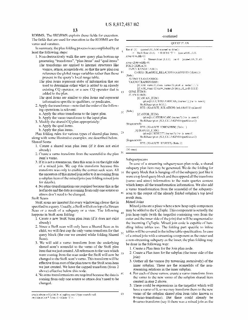
Plan folding rules for various types of shared plan items, along with some illustrative examples, are described below. Shared Scans
1. Create a shared scan plan item (if it does not exist already)
2. Create a varno transform from the scanrelid to the plan items varno.
3. If it is not a streamscan, then this scan is on the right side of a mixed join. We cap this transform because this transform was only to enable the correct seek scan. All the ancestors of this mixed join refer to it as coming from a Subplan item of the mixed join (see folding mixed join for details).
4. No attno transformations are required because this is the leafnode and the data is coming from only one source so attnos don’t need to be changed.
StoR Scans StoR scans are inserted for every windowing clause that is
specified in a query. Usually, a StoR will sit on top of a Stream Scan or a result of a subquery or a view. The following happens in StoR scan folding:
1. Create a new StoR Scan plan item (if it does not exist already)
2. Since a StoR scan will only have a Shared Scan as its child, we will first cap the only varno transform for that query block (the one we created while folding Shared Scan).
3. We will add a varno transform from the underlying shared scans scanrelid to the varno of the StoR plan item that we just created. All references to the vars which were coming from the scan under the StoR will now be changed to the StoR scans varno. This transform will be effective from root of the plan tree to the StoR scan item we just created. We have the capped transform (from 2 above) effective below this node.
4. No attno transformations are required because the data is coming from only one source so attnos don’t need to be changed.
create stream r1 (aint, bint cqtime user) type unarchived; explain select * from r1 <slices 3 >:
10
15
25
30
35
40
45
50
55
60
65
14 -continued
QUERY PLAN
Result (1) (cost=0.00.0.00 rows=0 width=0) -> StoR Scan (1.1) < SLICES 3’ > (cost=0.00.0.00
rows=0 width=0) -> Stream Scan (1.1.1)
rows=2140 width=8) FOLD EXPLAIN: INPUTRANGE TABLE:
(1) RTE: (Kind:RTE RELATION) (relid:81933) (alias:r1) (Rels:) ATTNO TRANSFORMS: WARNOTRANSFORMS:
1 (old varno: 1) (new varno: 1) (start at node:1.1.1) 2 (old varno: 1) (new varno:2) (stop at node:1.1.1)
QUALITEMS: PLANITEMS:
1) (SCAN ITEM) plan: 1.1.1 STREAMSCAN) (varno: 1) (rte is new:t)
StoRDescriptor: NULL RTE: (Kind:RTE RELATION) (relid:81933) (alias:r1)
on r1 (cost=0.00.31.40
(Rels:) 2) (STOR ITEM)
plan:1.1 STORSCAN) (varno:2) (rte is new:t) StoRDescriptor: (SD CHUNKING) (partitions:0)
(fragments:0) RTE: (Kind:RTE UNKNOWN) (Rels: 1)
(3) (RESULT ITEM) plan: 1 RESULT) (varno:3) (rte is new:t)
StoRDescriptor: (SD CHUNKING) (partitions:0) (fragments:0)
RTE: (Kind:RTE RESULT) (Rels: 2)
(26 rows)
Subqueryscans In case of a streaming Subquery scan plan node, a shared
subquery plan item may be generated. We do the folding for the query block that is hanging off of the Subquery just like it were atop level query block and then append all the transform (varno and attno) information to the main queries context which keeps all the transformation information. We also add a varno transformation from the scanrelid of the Subquery scan to the output of the already folded subplans top level result item. Mixed Joins Mixed joins are a place where a new heap tuple component
may be added to the CdTuple. This component is actually the join heap tuple (with the targetlist containing vars from the outer and the inner side of the join) that will be augmented to the incoming CdTuple. Mixed join code is capable of han dling inline tables too. The folding part specific to inline tables will be covered in the inline table specification. In case of a mixed join with a streaming component as the outer and a non-streaming subquery as the inner, the plan folding may be done in the following way:
1. Create a Plan item for the Join plan node. 2. Create a Plan item for the subplan (the inner side of the
join) 3. Gather all the varnos (by traversing recursively) of the
inner subplan. These are the scanrelids of the non streaming relations in the inner Subplan.
4. For each of these varnos, create a varno transform from the varno to the new varno of the subplan shared item created in step 2 above.
5. There could be expressions in the targetlist which will have a varno of 0, so we may transform them to the new Varno of the Subplan shared plan item (also known as 0-varno-transforms). But there could already be 0-varno-transform (say it there was a mixed join as the

US 8,812,487 B2 15
outer child of this current mixed join). We may cap these 0-varno-transforms to be effective only from the outer plan of the mixed join.
6. Now, we add a 0-varno-transform from 0 to the sunplan shared items varno. This will be effective from the root of the plan tree till the join node.
7. The join heap tuple (that will be augmented to the CdTuple), will have varnos from both inner and outer. Hence the attnos for these vars will be relative to the inner or the outer. We add attno transforms so that their attnos are correct when referred to the new varno that represents the entire join heaptuple. We may, for example, not alter the attnos of any vars that come from the outer since these vars will be accessed from the outer part of the CdTuple. We add attno transforms for all inner vars in the following way. If the oldattno is non Zero (regular var), then we change it to the position in the targetlist of the join. However, if the oldattno is zero, signifying it is an expression, there could be more than one expression and then we would wipe out the effects of all but the last attno transform. As such, a transform from 0 to the index in the target list may not be added. Hence, if the oldattno is zero then we copy the varattno to the oldattno field as a part of the attno transform.
create stream S1 (aint, bint, c int cqtime user) type unarchived; create table t1 (aint, b int): create index t1 a idx on t1 (a): explain selects.c, s.a., (s.a + S.c) as Sum1,
t.a, t.b, (t. b + s.c.) as Sum2 from S1 s, t1 t where s.a = t.a order
QUERY PLAN
Result (1) (cost=2790.96.2842.85 rows=20758 width=16) -> Sort (1.1) (cost=2790.96.2842.85 rows=20758
width=16) Sort Key: ((t. b + s.c)) -> Nested Loop (1.1.1)
rows=20758 width=16) -> StoR Scan (1.1.1.1) < SLICES 1 ROWS >
(cost=0.00.0.00 rows=0 width=0) -> Stream Scan (1.1.1.1.1)
(cost=0.00.29.40 rows=1940 width=8) -> Index Scan (1.1.1.2) using t1 a idx on
(cost=0.00.0.47 rows=11 width=8) Index Cond: (t.a = s.a.)
(cost=0.00.1302.47
on S1 S
FOLD EXPLAIN: INPUTRANGE TABLE:
(1) RTE: (Kind:RTE RELATION) (relid:81936) (alias:s) (Rels:)
(2) RTE: (Kind:RTE RELATION) (relid:81939) (alias:t) (Rels:)
ATTNO TRANSFORMS:
5
10
15
25
30
35
40
45
50
1
i WARNOT
(start at no
(stop at no
(start at no
(stop at no
(stop at no QUAL PLAN
(varno:0 oldattno:0 newattno:0) (varno:2 oldattino: 1 newattno:4) (varno:2 oldattno:2 newattno:5) (varno:0 oldattno:0 newattno:0) TRANSFORMS:
(old varno: 1) (new varno: 1) :1.1.1.1.1) (old varno: 1) (new varno:2)
:1.1.1.1.1) (old varno:2) (new varno:3)
:1.1.1.2) (old varno:2) (new varno:5)
:1.1.1.2) (old varno:0) (new varno:5)
:1.1.1.2) EMS:
(SCAN ITEM)
(stop:1.1.1.1) (stop:1.1.1.1) (stop:1.1.1.1) (stop:1.1.1.1)
(plan: 1.1.1.1.1 STREAMSCAN) (varno: 1)
55
60
65
16 -continued
(rte is new:t) StoRDescriptor: NULL
RTE: (Kind:RTE RELATION) (relid:81936) (alias:s) (Rels:)
2 (STOR ITEM) plan: 1.1.1.1 STORSCAN) (varno:2) (rte is new:t)
StoRDescriptor: (SD CHUNKING) (partitions:0) (fragments:0)
RTE: (Kind:RTE UNKNOWN) (Rels: 1) 3) (SCAN ITEM)
plan: 1.1.1.2 INDEXSCAN) (varno:3) (rte is new:t) StoRDescriptor: NULL
RTE: (Kind:RTE RELATION) (relid:81939) (alias:t) (Rels:)
4] (JOIN ITEM) plan: 1.1.1. NESTLOOP) (varno:4) (rte is new:t)
(parent:5) StoRDescriptor: (SD CHUNKING) (partitions:0)
(fragments:0) RTE: (Kind:RTE JOIN) (jointype:JOIN INNER) (Rels:)
5 (SUBPLAN ITEM) plan: 1.1.1.2 INDEXSCAN) (varno:5) (rte is new:t)
(Subplan:4) StoRDescriptor: NULL
RTE: (Kind:RTE SUBQUERY) (Rels:) (6) (RESULT ITEM)
plan: 1 RESULT) (varno:6) (rte is new:t) StoRDescriptor: (SD CHUNKING) (partitions:0)
(fragments:0) :RTE RESULT) (Rels: 25)
(51 rows)
Shared Aggs Shared Agg items are created when an agg or an agg sitting
on top of one or more of the following plan nodes is encoun tered:
Unique Sort Limit Group An agg node combined with Zero or more of these plan
nodes may form an “agg chain.” We will create a shared plan item for the entire agg chain. The output of an agg is a combination of grouping columns (optional—only for groupedaggregates) and aggrefs (for grouped and ungrouped aggregates). All input varno and attno references may be changed in the following way:
1. An agg plan item is created. 2. The existing transformations are capped so that they are
only effective below the agg chain. 3. All aggrefs have a varno of 0. A varno transform is added
from 0 to the varno of the newly created agg plan item. 4. For these agg refs, we also are add attno transform to
copy the varattno field to varoldattno in the vars. 5. For grouping columns, the old varnos for the input to the
agg chain may be pulled and a varno transform for each of these varnos may be created. These varno transforms will be from the oldvarno to the new varno of the shared agg item
6. For all the old varnos of the grouping columns we add attno transforms to copy the varattno field to the varol dattno field.
7. All these transformations mentioned above (varno and attno) will be effective from root of the plan tree till the start of the agg chain.
explain selecta, count(*) from r1 <slices 3 > group by a: QUERY PLAN

US 8,812,487 B2 17
-continued
Result (1) (cost=0.00.2.50 rows=200 width=0) -> HashAggregate (1.1) (cost=0.00.2.50 rows=200
width=0) -> StoR Scan (1.1.1) < SLICES 3’ >
(cost=0.00.0.00 rows=0 width=0) -> Stream Scan (1.1.1.1) on r1
(cost=0.00.31.40 rows=2140 width=4) FOLD EXPLAIN: INPUTRANGE TABLE:
(1) RTE: (Kind:RTE RELATION) (relid:81933) (alias:r1) (Rels:)
ATTNO TRANSFORMS: 1 (varno:0 oldattno:0 newattno:0) 2 (varno: 1 oldattino:0 newattno: 0)
WARNOTRANSFORMS: (old varno: 1) (new varno: 1)
e:1.1.1.1) 2 (old varno: 1) (new varno:2) (start at node:1.1) e:1.1.1.1) 3 (old varno:O) (new varno:3) (stop at node:1.1) 4 (old varno: 1) (new varno:3) (stop at node:1.1)
(stop:1.1) (stop:1.1)
(start at no
(stop at no
QUALITEMS: PLAN ITEMS:
(SCAN ITEM) plan: 1.1.1.1 STREAMSCAN) (varno: 1)
(rte is new:t) StoRDescriptor: NULL
RTE: (Kind:RTE RELATION) (relid:81933) (alias:r1) (Rels:)
2 (STOR ITEM) plan: 1.1.1 STORSCAN) (varno:2) (rte is new:t)
StoRDescriptor: (SD CHUNKING) (partitions:0) (fragments:0)
RTE: (Kind:RTE UNKNOWN) (Rels: 1) (3) (AGG ITEM)
plan:1.1AGG) (varno:3) (rte is new:t) (stop:1.1AGG)
StoRDescriptor: (SD CHUNKING) (partitions:0) (fragments:0)
RTE: (Kind:RTE AGGREGATE) (Rels: 2) (4) (RESULT ITEM)
plan: 1 RESULT) (varno:4) (rte is new:t) StoRDescriptor: (SD CHUNKING) (partitions:0)
(fragments:0)
(35 rows)
Shared Result Shared Result items are created when we encounter either
a result node or a result node sitting on top of one or more of the following plan nodes:
Unique Sort Limit Group A result node combined with Zero or more of these plan
nodes may comprise an “result chain.” We will create a shared plan item for the entire result chain. Result nodes can be either on the top of the query plan, or introduced in the middle of a query block for projection purposes. For a top level result node, we do not need any transformations. But if a result node is not the topmost node of a query block we may do the following:
1. Cap all the existing varno transforms so that they are effective only below the result chain.
2. Pull all the old varnos of the vars from the targetlist of the result node. Add a varno transform for each of these old varnos. The new varno will be the varno of the newly created Result shared planitem.
3. Add an extra varno transform (0-varno-transform) from 0 to the varno of the result shared plan item for any exprs, COnStS etc.
10
15
25
30
35
40
45
50
55
60
65
18 4. Add attno transforms for the columns since we have
mostly done projections in this result node. If the old attno is non-zero (regular var), then we change it to the position in the targetlist of the join. However, if the oldattno is Zero, signifying it is an expression, it will be wrong to add a transform from 0 to the index in the targetlist because there could be more than one expres sions and then we would wipe out the effects of all but the last attno transform. Hence, if the oldattno is zero then we copy the varattno to the oldattno field as a part of the attno transform.
5. All these transformations mentioned above (varno and attno) will be effective from root of the plan tree till the start of the result chain.
create stream res(a int, bint, t timestamp cqtime user) type unarchived; explain select * from res<slices 1 rows> where a = 3 limit
QUERY PLAN
(cost=0.00.0.00 rows=1 width=0) (cost=0.00.0.00 rows=1 width=0)
(cost=0.00.0.00 rows=0
Result (1) -> Limit (1.1)
-> Result (1.1.1) width=0)
-> StoR Scan (1.1.1.1) (cost=0.00.0.00 rows=0 width=0)
Filter: (a = 3) -> Stream Scan (1.1.1.1.1)
(cost=0.00.32.12 rows=9 width=16)
< SLICES 1 ROWS >
Oil (S
FOLD EXPLAIN: INPUTRANGE TABLE:
(1) RTE: (Kind:RTE RELATION) (relid:81947) (alias:res) (Rels:)
ATTNO TRANSFORMS: 1 (varno:1 oldattino: 1 newattno: 1) (stop:1.1.1) 2 (varno:1 oldattno:2 newattno:2) (stop:1.1.1) 3 (varno: 1 oldattino:3 newattno:3) (stop:1.1.1)
WARNOTRANSFORMS: 1 (old varno: 1) (new varno: 1)
(start at node: 1.1.1.1.1) 2 (old varno: 1) (new varno:2) (start at node:1.1.1)
(stop at node:1.1.1.1.1) 3 (old varno: 1) (new varno:3) (stop at node:1.1.1) 4 (old varno:O) (new varno:3) (stop at node:1.1.1)
QUALITEMS: QualItem (plan:1.1.1.1)
PLANITEMS: 1) (SCAN ITEM)
plan: 1.1.1.1.1 STREAMSCAN) (varno: 1) (rte is new:t)
StoRDescriptor: NULL RTE: (Kind:RTE RELATION) (relid:81947) (alias:res)
(Rels:) 2) (STOR ITEM)
plan: 1.1.1.1 STORSCAN) (varno:2) (rte is new:t) StoRDescriptor: (SD CHUNKING) (partitions:0)
(fragments:0 ) RTE: (Kind:RTE UNKNOWN) (Rels: 1) 3) (RESULT ITEM)
plan: 1.1.1 RESULT) (varno:3) (rte is new:t) StoRDescriptor: (SD CHUNKING) (partitions:0)
(fragments:0 ) RTE: (Kind:RTE RESULT) (Rels: 2) 4 (RESULT ITEM)
plan: 1 RESULT) (varno:4) (rte is new:t) StoRDescriptor: (SD CHUNKING) (partitions:0)
(fragments:0) :RTE RESULT) (Rels: 3)
Orchestrating Iterator-Model Sub-Plans for Streaming A technique that permits a quick and easy reuse of RDBMS
infrastructure in an SRDBMS is disclosed as follows:
US 8,812,487 B2 19
The SRDBMS evaluates standard relational operations (e.g., filters, joins, aggregates, sort) on streaming data using the special CQ operators. Although these CQ operators are conceptually similar to the IMP operators of a traditional RDBMS their underlying interfaces are significantly differ ent. An SRDBMS can achieve streaming versions of standard relational operations by reusing the standard IMP implemen tation of the underlying RDBMS, and goes beyond just reus ing Smaller components such as an expression evaluator—the idea is to take full advantage of mature and efficient technol ogy Such as outer join implementation.
In essence, a CO operator focuses on managing streaming data as well as sharing information and orchestrates the underlying IMP sub-plan to achieve the actual relational operations. The techniques to address the situation posed above as
described above may include but is not limited to the follow 1ng: As part of plan folding the input IMP plan is chopped up
into various Sub-plans, each of which is placed under the control of a specific CO operator. In a sense, each CO operator now contains an independent IMP executor.
A new leaf node, an Adapter, is added to the IMP sub-plan. The Adapter is an iterator-model operator and serves as a way to bridge the CQ operator and the IMP sub-plan. In essence, the Adapter fetches one or more CQ tuples from the controlling CQ operator and delivers it to its parents.
As a result of plan folding, the expressions evaluated by the operators in the IMP sub-plan can work seamlessly on a composite CQ tuple in most cases. In certain circum stances, however, an IMP operator may access the attributes of an input tuple directly and not through the expression evaluator. In such situations the Adapter projects the composite CO tuple into a traditional tuple so that it can be evaluated by the IMP sub-plan.
When the CQ operator is called with a new CQ tuple, it evaluates the appropriate logic (e.g., has a window edge has been triggered) and does one or more of the follow ing depending on the actual operator: Buffer the CQ tuple in local state Call the next()method on the root of the IMP sub-plan
and deliver one or more tuples through the Adapter
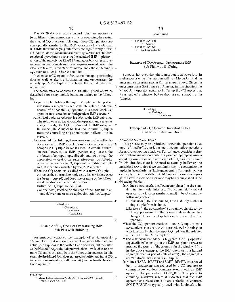
Mixed Join -> Nested Loop
-> Adapter -> IndexScan
Example of CQ Operator Orchestrating IMP Sub-Plan with Buffering
For instance, consider the example of a stream-table “Mixed Join' that is shown above. The heavy lifting of the actual join happens in the Nested Loop operator, but the outer of the Nested Loop is the Adapter which in turn fetches one or more CQ tuples at a time from the Mixed Join operator. In this example the Mixed Join does not need to buffer any input CQ tuple and can insteadjust call the next() method on the Nested Loop operator.
Mixed Join -> Merge Left Join (cost=299.56.653.73 rows=22898 width=8)
Merge Cond: (f.b = b.c)
10
15
25
30
35
40
45
50
55
60
65
20 -continued
-> Sort (Sort Key: fb) -> Adapter
-> Sort (Sort Key: b.c) -> Seq Scan on barb
Example of CQ Operator Orchestrating IMP Sub-Plan with Buffering
Suppose, however, the join in question is an outer join. In Such a scenario the join operator will be a Merge Join and the inner and outer arms need a Sort as shown above. Since the outer arm has a Sort above an Adapter, in this situation the Mixed Join operator needs to buffer up the CQ tuples that form part of a window before they are consumed by the Adapter.
Shared Agg -> HashAgg
-> Adapter
Example of CQ Operator Orchestrating IMP Sub-Plan with Accumulation
Advanced Solution Device This process may be optimized for certain operations that
may be found in CO queries, namely accumulative operations for non-overlapping windows. For instance, consider a situ ation where we are computing a grouped aggregate over a chunking window on a stream as part of a CO as shown above. In this situation there is no need to actually buffer up the individual CQ tuples if we can find a way to accumulate the tuples in the underlying HashAgg operator. This optimization can apply to various different IMP operators such as aggre gates as well as sort operators and may be accomplished in the following fashion:
Introduce a new method called accumulate() to the stan dard iterator model interface. The accumulate()method operates in a fashion similar to next(). by obeying the following contract: Unlike next(), the accumulate() method only fetches a
single tuple from its input. Like next(), the accumulate() dispatcher checks to see
if any parameter of the operator depends on has changed. If so, the dispatcher calls rescan () on the operator.
When the CQ operator receives a new CQ tuple it calls accumulate() on the root of its associated IMP sub-plan which in turn fetches the input CQ tuple via the Adapter at the leaf of the IMP sub-plan.
When a window boundary is triggered the CQ operator repeatedly calls next() on the IMP sub-plan in order to produce the results of the operator for the window. If, as in the above example, the IMP operator is a hashed aggregate then as part of calls of next() the aggregates are “finalized for use in result tuples.
Introduce HARD RESET and SOFT RESET, two special built-in parameters that are used by a CO operator to communicate window boundary events with an IMP operator. In particular, HARD RESET applies to chunking windows where it indicates that the IMP operator can clean out its state entirely. In contrast, SOFT RESET is typically used with landmark win

US 8,812,487 B2 21
dows in order to indicate to the IMP operator that its actual underlying internal state (based on user data) should be preserved although the associated controlling data structures (e.g., list/hash-table iterators) can be reset.
The accumulating device described above can also be used for operators such as Sort and Bounded Sort in addition to Aggregates. Windowing Infrastructure The following set of techniques may be used to implement
various different types of StoRs (StreamToRelation operators or windows) in a unified manner. The streaming query processing includes an ability to
divide the infinite stream of data into “windows' and perform different kinds of operation on them. In an SRDBMS, we achieve this by converting the stream into window sized rela tions and then performing all other operations on these rela tions. We call the operators that dissect the stream into win dows as StoRs (for Stream to Relation). A unified windowing infrastructure may solve the follow
1ng: Support multiple kinds of windows (chunking, sliding,
landmark) whose parameters can in turn be based on different concepts (time, rows, windows).
Eliminate additive latency. When CQs are stacked up in a chain, the prior art implementation results in a latency that is the sum of the advance intervals of each Succes sive query in the chain.
The techniques to address the situation posed above as described above may include but is not limited to the follow 1ng: Data and Control Tuples The raw stream is a sequence of data tuples. The way we
choose to implement StoRS is by punctuating the tuples of the raw stream with special control information that will denote the window edges. These tuples are called Control tuples. Therefore, the StoR operators will usually be the first operator that tuples from a raw stream will go to. Once the raw stream has passed through the StoR, it will contain data as well as control tuples. There could be multiple StoRs in a query (if we have a view, a subquery etc.). In Such cases, the stream that contains the data and control tuples can pass through one or more StoRs downstream. Therefore, the StoRs are equipped to handle data as well as control tuples in their incoming stream while they inject their control tuples. Window Edges and their Advance Kinds
Ever window has two edges—the leading edge and the trailing edge. The heart of the operation of a StoR is to detect when an edge is triggered so that it can insert a control tuple signifying the existing of an edge. The advancement of these edges can be based either on time (the non-decreasing value in cqtime column of the stream), or on number of rows, or on the number of windows seen coming from an underlying subquery. We will call these different advance kinds as advance-by-time, advance-by-row and advance-by-windows respectively.
All three types of windows (landmark, chunking and slid ing) may have the same mechanism of triggering the leading edge (specified by the slices clause in chunking windows or advance’ clause in landmark and sliding windows). They will, however, differ a little on when their trailing edges are inserted. Edge Triggering Logic The basic edge triggering logic includes comparing the
value of an attribute (for advance-by-time it is the cqtime column, for advance-by-rows it is the rowcount, for advance by-windows it is the window id) of a new incoming tuple with
10
15
25
30
35
40
45
50
55
60
65
22 the value of the next edge. All the tuples with the value of the attribute less than or equal to the value of the next edge belong to the window that is being formed. The edge triggering logic differs slightly based on the advance kind of the edge. When we are advancing by time, we use the value of the cqtime attribute of the stream whereas, when advancing by rows we use the rowcount. While any data tuple can have the same value of cqtime as its previous one, it may not have the same rowcount. Therefore, for advance-by-time, we cannot trigger an edge unless we have seen a tuple that has a cqtime that is greater than the value of the next edge. In contrast, when we are advancing by rows, we can trigger an edge when we see a tuple with rowcount that is equal to the next edge of the window. For advance-by-windows, we compare the window id in the control tuple with the value of the next edge. Since two windows may not have the same window id, it is similar to advance-by-rows in that we can close a window in a Super query that is advancing by windows if we see a control tuple from a subquery that denotes a leading edge and that has a window id equal to the next edge of the superquery's StoR.
Following is an exemplary algorithm for triggering an edge:
bool edge triggered (next edge, input tuple attribute, input tuple type)
* the input tuple attribute can be cqtime of the input tuple for * advance-by-time or rowcount of the input tuple for * advance-by-rows. It will be the window id of incoming tuple * for advance-by-windows.
if (GetAdvanceKind (next edge) == advance-by-time)
if (input tuple attribute > GetValue(next edge)) return true:
else if (GetAdvanceKind(next edge) == advance-by-rows) {
Assert(input tuple attribute <= GetValue(next edge)); if (input tuple attribute == GetValue(next edge))
return true:
else f* advance-by-windows */ {
Assert(input tuple attribute <= GetValue(next edge)); if (IsLeadingEdgeControlTupleType(input tuple type) &&.
input tuple attribute == GetValue(next edge)) return true:
return false:
StoR Execution Logic for Leading Edge As mentioned earlier, the execution logic for leading edge
may be the same for all the types of windows. When we have advance-by-time, if we get an input tuple that does not trigger the edge, we route it along to the downstream operators. If, however, a tuple comes after some time, it can trigger one or more edges and we send control tuples representing all the intermediate leading edges and then route the tuple to down stream operators. The input tuple is routed after the control tuple(s) because it has a timestamp greater than the window edge that we are closing so it belongs to the next window. For advance-by-rows, if we get an input tuple that does not trigger an edge, we route it along to the downstream operators. If we get a tuple that triggers an edge (we may trigger one edge in advance-by-rows or advance-by-windows), we route the data tuple and then route the control tuple signifying end of the

US 8,812,487 B2 23
window. This is because the input tuple belongs to the win dow that we are about to close.
Following is the algorithm for StoR execution of leading edge:
void execute StoR (stor state, input tuple)
{ control tuple = NULL; input tuple type = GetTupleType(input tuple); next edge = GetLeadingEdge(stor state); /* Get input tuple attribute */ if (GetAdvanceKind(next edge) == advance-by-rows)
input tuple attribute = GetRowCount(input tuple); else if (GetAdvanceKind (next edge) == advance-by-time)
input tuple attribute = GetCdTime(input tuple); else
input tuple attribute = GetWindowId(input tuple); while (edge triggered (next edge,
input tuple attribute, input tuple type)
)
ContructControlTuple(control tuple); if (GetAdvanceKind(next edge) == advance-by-time)
RouteTuple(control tuple); control tuple = NULL;
AdvanceEdge(next edge); f* end of edge triggered while loop */
/* Route data tuple */ if (IsData TupleType(input tuple type))
RouteTuple(input tuple); f* Route control tuple in case of advance by
rows windows */ if (control tuple l= NULL)
RouteTuple(control tuple);
StoR Execution Logic for Trailing Edges The various window types differ in how the trailing edges
of their windows are emitted. Following is the execution logic specific to each window type. Chunking Windows
Chunking windows, by definition are contiguous. Hence, there is no need to explicitly emit a trailing edge, because the leading edge of window can be interpreted as the trailing edge of the next window. The trailing edge of a chunking window will have the same
advance kind as the leading edge. A data tuple cannot be a part of more than one chunking
window. Landmark Windows The trailing edge of a landmark window is triggered based
on the input tuple's relevant attribute (cqtime for advance-by time, rowcount for advance-by-rows, and window id for advance-by-windows) with respect to the next edge calcu lated by what was specified in the RESET clause. The trailing edge triggering logic is very similar to the
leading edge logic except that it works independently and orthogonal to the leading edge. So, an input tuple can trigger one or both of the edges. The trailing edge of a landmark window can have an
advance kind that is different from its leading edge. A data tuple may be a part of multiple windows because all
windows will have different leading edges but the same trail ing edge until a trailing edge (RESET) is triggered. Sliding Windows
For sliding windows, trailing edges cannot be triggered independently (unlike landmark windows), because the trail ing or visible edge of a window is calculated backwards
10
15
25
30
35
40
45
50
55
60
65
24 from the leading or advance edge and the advance kind of each edge can be different. Since, trailing edge of a window should precede the leading edge, but we cannot emit a trailing edge till we are about to emit a leading edge, we encode the information about the trailing edge in the control tuple that is emitted for the leading edge. The downstream operators are responsible for buffering the tuples and extracting the embed ded information about the trailing edge from the control tuple. This information can be used to discard the buffered tuples that don't belong to the window. A data tuple can be part of multiple sliding windows. Depending on the advance kind of the visible clause, we
embed the trailing edge information inside the control tuple differently.
If the trailing edge is advance-by-rows then when we emit the control tuple for the leading edge we populate the trailing edge information field with (R-V) where, R is the rowcount of the control tuple for leading edge and V is the number of rows specified in the visible clause.
If the trailing edge is advance-by-time then when we emit the control tuple for the leading edge we populate the trailing edge information field with (T-V) where T is the cqtime of the control tuple for leading edge and V is the time specified in the visible clause.
Solution for the Additive Lag Problem When we are advancing by time, we cannot trigger a win
dow edge until we have seen a tuple that has a cqtime greater than the next edge value. This can potentially lead to an additive lag in some cases when we have both Subqueries and Superqueries advance by time.
Example: Let us say that the subquery StoR is slices 3 seconds and the Superquery StoR is slices 5 seconds. The windows from the subquery will be 3 seconds apart. Let us assume that the rows from the subquery come at times 3, 6, 9... seconds. The superquery will close its first window (next edge being 5) when it sees the first tuple with timestamp 6. Though the subquery finished its 3 second window, the super query could not close its 5 seconds window because it did not See any tuple with cqtime greater than 5. The Superquery had to wait till the Subquery was done finishing the 6 second window to close its 5 second window. Thus, we had a lag of 3 seconds. If we have many levels of nesting, this lag could very quickly add up making the streaming applications prohibi tively slow.
This problem of additive lag is solved by having specula tive time in control tuples. Speculative Time in Control Tuples
In order to reduce the additive lag described above, we introduced a concept of adding a speculative time in the control tuples for leading edges of advance-by-time win dows. When we emit a leading edge, we send a control tuple with cqtime as the window edge time. We also populate an extra field in the control tuple—called the speculative time with the value of the next window edge. By doing this, we are informing the consumer of this control tuple that the next data that comes out of the subquery will have a cqtime of the next window edge. In the above example, the control tuple ending the 3 second window will have a speculative time of 6. When the Superquery, sees a control tuple with speculative time of 6 it knows that it cannot see any data that will have acqtime less than or equal to 5 hence it can close the 5 second window as Soon as the Subquery's 3 second window has ended. The edge triggering logic in advance-by-time windows
will change slightly. When we are advancing by time, if we get an input tuple that is a control tuple we use the speculative time as the input tuple attribute instead of the cqtime of the tuple to check if an edge can be triggered.
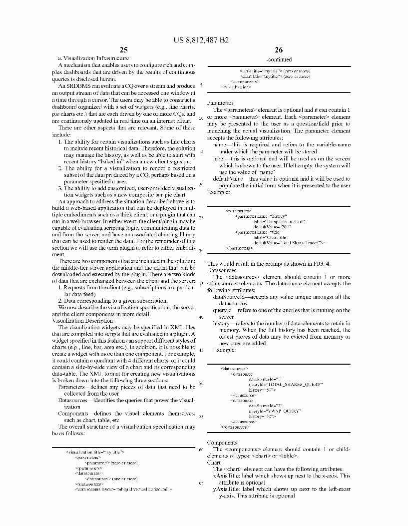
US 8,812,487 B2 25
a. Visualization Infrastructure A mechanism that enables users to configure rich and com
plex dashboards that are driven by the results of continuous queries is disclosed herein. An SRDBMS can evaluate a CO over a stream and produce 5
an output stream of data that can be accessed one window at a time through a cursor. The users may be able to construct a dashboard organized with a set of widgets (e.g., line charts, pie charts etc.) that are each driven by one or more CQS, and are continuously updated in real time on an internet client.
There are other aspects that are relevant. Some of these include:
1. The ability for certain visualizations such as line charts to include recent historical data. Therefore, the solution may manage the history, as well as be able to start with recent history “baked in when a new client signs on.
2. The ability for a visualization to render a restricted subset of the data produced by a CO, perhaps based on a parameter specified a user.
3. The ability to add customized, user-provided visualiza tion widgets such as a new composite bar-pie chart.
An approach to address the situation described above is to build a web-based application that can be deployed in mul tiple embodiments such as a thick client, or a plugin that can run in a web browser. In either event, the client/plugin may be capable of evaluating scripting logic, communicating data to and from the server, and have an associated charting library that can be used to render the data. For the remainder of this section we will use the term plugin to refer to either embodi ment.
There are two components that are included in the solution: the middle-tier server application and the client that can be downloaded and executed by the plugin. There are two kinds of data that are exchanged between the client and the server:
1. Requests from the client (e.g., Subscriptions to a particu lar data feed)
2. Data corresponding to a given Subscription. We now describe the visualization specification, the server
and the client components in more detail. Visualization Description The visualization widgets may be specified in XML files
that are compiled into Scripts that are evaluated in a plugin. A widget specified in this fashion can support different styles of charts (e.g., line, bar, area etc.). In addition, it is possible to create a widget with more than one component. For example, it could contain a quadrant with 4 different charts, or it could contain a side-by-side view of a chart and its corresponding data-table. The XML format for creating new visualizations is broken down into the following three sections:
Parameters—defines any pieces of data that need to be collected from the user
DataSources—identifies the queries that power the visual ization
Components—defines the visual elements themselves, Such as chart, table, etc
The overall structure of a visualization specification may be as follows:
10
15
25
30
35
40
45
50
55
<visualization title="my title'> 60 <parameters>
<parameterf> (zero or more) <?parameters> <dataSources>
<dataSourcef> (one or more) <datasources> 65 <components layout="tablgrid vertical horizontal's
26 -continued
<table title="mytitle> (zero or more) <chart title="mytitle> (zero or more)
</components-> </visualization
Parameters The <parameters> element is optional and it can contain 1
or more <parameters element. Each <parameters element may be presented to the user as a question/field prior to launching the actual visualization. The parameter element accepts the following attributes: name—this is required and refers to the variable-name
under which the parameter will be stored label this is optional and will be used as on the screen
which is shown to the user. If left empty, the system will use the value of name
defaultValue—this value is optional and it will be used to populate the initial form when it is presented to the user
Example:
<parameters> <parameter name="history
label="Datapoints in chart defaultValue="200
<parameter name="title label="Chart title defaultValue="Total Shares Traded's
<?parameters>
This would result in the prompt as shown in FIG. 4. DataSources The <datasources element should contain 1 or more
<dataSource> elements. The dataSource element accepts the following attributes:
dataSourced—accepts any value unique amongst all the dataSources
queryId-refers to one of the queries that is running on the Sever
history—refers to the number of data-elements to retain in memory. When the full history has been reached, the oldest pieces of data may be evicted from memory as new ones are added
Example:
<dataSources.> <dataSource
dataSourced='1' queryId="TOTAL SHARES QUERY history="50">
<datasource> <dataSource
dataSourced=2 queryId=*VWAP QUERY history="50">
<datasource> <datasources
Components The <components element should contain 1 or child
elements of types: <chart or <table>. Chart The <chart element can have the following attributes: XAxisTitle: label which shows up next to the x-axis. This
attribute is optional y AxisTitle: label which shows up next to the left-most
y-axis. This attribute is optional
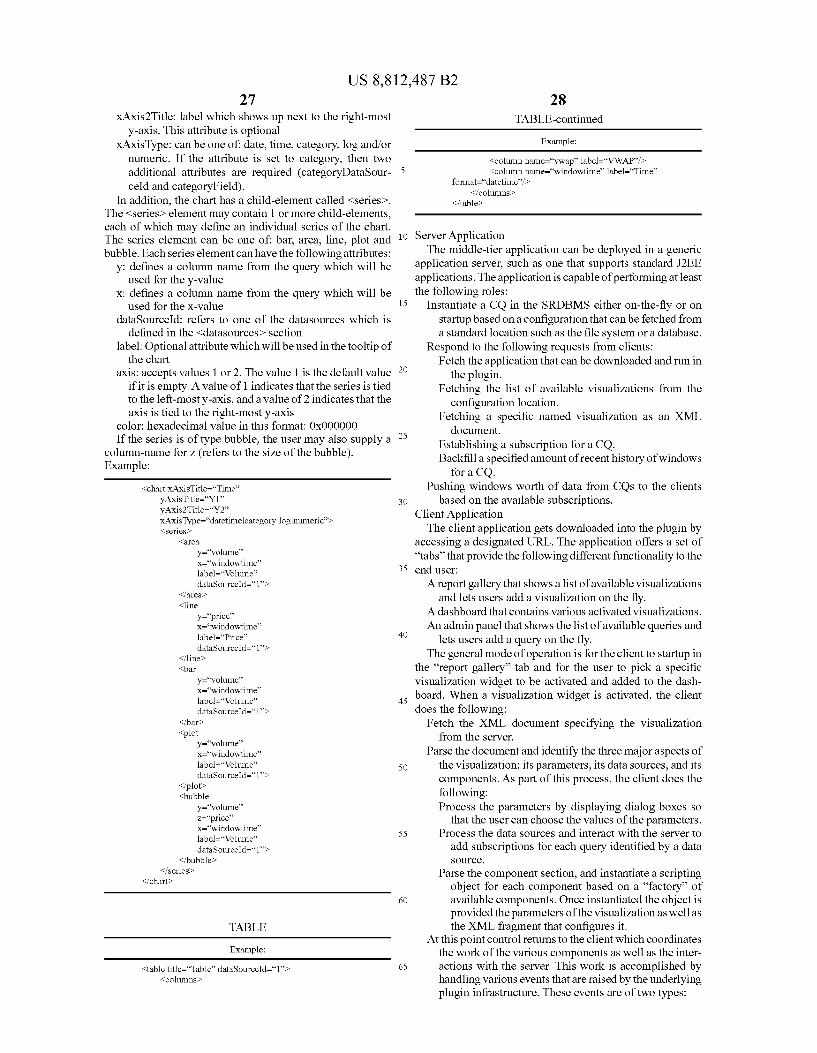
US 8,812,487 B2 27
XAxis2Title: label which shows up next to the right-most y-axis. This attribute is optional
XAXisType: can be one of date, time, category, log and/or numeric. If the attribute is set to category, then two additional attributes are required (categoryDataSour celd and categoryField).
In addition, the chart has a child-element called <series. The <series.> element may contain 1 or more child-elements, each of which may define an individual series of the chart. The series element can be one of bar, area, line, plot and bubble. Each series element can have the following attributes:
y: defines a column name from the query which will be used for the y-value
X: defines a column name from the query which will be used for the X-value
dataSourced: refers to one of the datasources which is defined in the <datasources section
label: Optional attribute which will be used in the tooltip of the chart
axis: accepts values 1 or 2. The value 1 is the default value if it is empty. A value of 1 indicates that the series is tied to the left-most y-axis, and a value of 2 indicates that the axis is tied to the right-most y-axis
color: hexadecimal value in this format: 0x000000 If the series is of type bubble, the user may also supply a
column-name for Z (refers to the size of the bubble). Example:
<chart X AxisTitle=''Time' y AxisTitle=Y1 y Axis2Title=“Y2 XAxisType="datetime category log numeric <series.>
<area y=“volume x="windowtime label="Volume dataSourced='1'>
<area <line
y="price' x="windowtime label="Price' dataSourced='1'>
<linex <bar
y=“volume x="windowtime label="Volume dataSourced='1'>
<barc> <plot
y=“volume x="windowtime label="Volume dataSourced='1'>
</plots <bubble
y=“volume z="price' x="windowtime label="Volume dataSourced='1'>
<bubble> <series.>
<chart
TABLE
Example:
<table title=''Table' dataSourced='1'> <columns
10
15
25
30
35
40
45
50
55
60
65
28 TABLE-continued
Example:
<column name="vwap label=“VWAP/> <column name="windowtime label="Time
format="datetime' > <columns
<?table>
Server Application The middle-tier application can be deployed in a generic
application server, Such as one that Supports standard J2EE applications. The application is capable of performing at least the following roles:
Instantiate a CO in the SRDBMS either on-the-fly or on startup based on a configuration that can be fetched from a standard location Such as the file system or a database.
Respond to the following requests from clients: Fetch the application that can be downloaded and run in
the plugin. Fetching the list of available visualizations from the
configuration location. Fetching a specific named visualization as an XML
document. Establishing a subscription for a CO. Backfill aspecified amount of recent history of windows
for a CO. Pushing windows worth of data from CQs to the clients
based on the available subscriptions. Client Application The client application gets downloaded into the plugin by
accessing a designated URL. The application offers a set of “tabs that provide the following different functionality to the end user: A report gallery that shows a list of available visualizations
and lets users add a visualization on the fly. A dashboard that contains various activated visualizations. An admin panel that shows the list of available queries and
lets users add a query on the fly. The general mode of operation is for the client to startup in
the “report gallery” tab and for the user to pick a specific visualization widget to be activated and added to the dash board. When a visualization widget is activated, the client does the following:
Fetch the XML document specifying the visualization from the server.
Parse the document and identify the three major aspects of the visualization: its parameters, its data sources, and its components. As part of this process, the client does the following: Process the parameters by displaying dialog boxes so
that the user can choose the values of the parameters. Process the data sources and interact with the server to add subscriptions for each query identified by a data SOUC.
Parse the component section, and instantiate a scripting object for each component based on a “factory' of available components. Once instantiated the object is provided the parameters of the visualization as well as the XML fragment that configures it.
At this point control returns to the client which coordinates the work of the various components as well as the inter actions with the server. This work is accomplished by handling various events that are raised by the underlying plugin infrastructure. These events are of two types:

US 8,812,487 B2 29
User interaction events that are found in standard event driven UIs. Examples include moving the mouse, clicking on something, navigating to a specific tab, etc.
Data update events that are raised when new data arrives from the server for an active subscription.
For either event, the client identifies the component script ing object that is responsible for handling it, and then dispatches the event to that object. The Scripting object is responsible for visually rendering the data communi cated to it using the underlying infrastructure provided by the plugin, such as charting.
Advanced Solution Device In the advanced version of the solution, the following may
be accomplished: Managing History A chart that needs history (e.g., a line chart) is configured
with an extra parameter describing the amount of history in terms of the number of windows that the chart may preserve. In this context an issue to be solved is the initial set of history data to be bound to the chart when it is first activated. This is accomplished by having the client request a backfill of data from the server while activating a chart. Restricting Data A visualization widget may render only a Subset of the
actual data that is produced by a CO. This may be for two CaSOS
1. In order to let a user control how the widget can manipu late a given data set in different ways, possibly control ling how much data is actually rendered in any given configuration. One common use for Such functionality is in order to “focus' on a subset of the data that the user has expressed interest in.
2. A given CO might produce a common set of results that might apply to multiple different visualization widgets. For instance, we might have a CO that produces Sum mary market information for multiple currency pairs, and the CQ serves as a data source for a visualization widget that is instantiated by different clients and with a different value for a parameter that restricts the data by currency pair. In Such a situation it is useful to annotate a Subscription on a data source with a restriction that is based on a specific parameter value.
While both of the situations above are similar they are used to accomplish different goals. In the former instance the goal is to fetch a single, possibly large, set of data from the server to the client and then winnow it in several different ways without going back to the server each time. In the latter instance the goal is to repeatedly fetch a limited set of data and avoid including any extraneous data that is known to be unnecessary at the client.
In either instance the idea is to annotate a data source specification with a “filter in the XML that defines a visual ization widget. There is an additional setting for the filter annotation which has two possible choices:
1. Run "on client’: This is suitable for the first situation described above where the client restricts the data being rendered but does not affect the actual data fetched from the server.
2. Run"on server’’: This is suitable for the second situation described above, and requires an extra communication step to the server application which in turn applies the filter for each data tuple produced by the CQ while processing the Subscription associated with a given data SOUC.
10
15
25
30
35
40
45
50
55
60
65
30 Extensibility Extensibility can be accomplished in two ways:
1. Where a user adds a custom component (e.g., a compos ite bar-pie chart) by adding an associated user-provided Scripting object and registering the association of the object to a specific tag in the visualization XML so that the factory can instantiate it.
2. Where a user modifies the functionality of an existing component (e.g., to add annotations to a chart) by imple menting a hook that gets invoked by the component factory when activating a component. The hook gets specified in the XML document that describes the visu alization widget.
The invention claimed is: 1. A method for managing a data stream, comprising: receiving a continuous query; generating an iterator-model plan based on the continuous
query; adding the continuous query to a shared continuous-query
plan by: analyzing the iterator-model plan and generating a plural
ity of iterator-model subplans by walking the iterator model plan bottom-up to generate transforms, plan items and qual items based on the iterator-model plan; and
for at least one particular iterator-model subplan of the plurality of iterator-model subplans:
assigning a continuous-query operator to the particular iterator-model Subplan; and
adding an adapter as a new leaf node to the particular iterator-model subplan, wherein the adapter is an itera tor-model operator configured to fetch one or more pro cessed continuous-query tuples from the continuous query operator and provide the one or more fetched continuous-query tuples to the particular iterator-model Subplan of the adapter;
applying the transforms to convert local range variables of the continuous query to global range variables; and
based on the plan items and the qual items, modifying the shared continuous-query plan, wherein the plan items refer to one or more new or existing continuous-query operator of the shared continuous-query plan, and wherein the qual items comprise information specific to at least one of qualifiers and predicates;
wherein the method is performed by one or more comput ing devices.
2. The method of claim 1, further comprising: providing the one or more processed continuous-query
tuples to the particular iterator-model Subplan. 3. The method of claim 1, wherein the continuous-query
operator operates on a stream. 4. The method of claim 1, wherein the shared continuous
query plan comprises a routing table encoding a plurality of routes for tuples in a shared dataflow, wherein adding the continuous query to the shared continuous-query plan further comprises modifying the routing table.
5. A non-transitory computer-readable medium storing instructions which, when processed by one or more proces SOrS, Cause:
receiving a continuous query; generating an iterator-model plan based on the continuous
query; adding the continuous query to a shared continuous-query
plan by: analyzing the iterator-model plan and generating a plural
ity of iterator-model subplans by walking the iterator
US 8,812,487 B2 31
model plan bottom-up to generate transforms, plan items and qual items based on the iterator-model plan; and
for at least one particular iterator-model subplan of the plurality of iterator-model subplans: 5
assigning a continuous-query operator to the particular iterator-model subplan; and
adding an adapter as a new leaf node to the particular iterator-model subplan, wherein the adapter is an itera tor-model operator configured to fetch one or more pro cessed continuous-query tuples from the continuous query operator and provide the one or more fetched continuous-query tuples to the particular iterator-model subplan of the adapter;
applying the transforms to convert local range variables of the continuous query to global range variables; and
based on the plan items and the qual items, modifying the shared continuous-query plan, wherein the plan items
10
32 refer to one or more new or existing continuous-query operator of the shared continuous-query plan, and wherein the qual items comprise information specific to at least one of qualifiers and predicates.
6. The non-transitory computer-readable medium as recited in claim 5, further comprising providing the one or more processed continuous-query tuples to the particular iterator model subplan.
7. The non-transitory computer-readable medium as recited in claim 5, wherein the continuous-query operator operates on a stream.
8. The non-transitory computer-readable medium as recited in claim 5, wherein the shared continuous-query plan comprises a routing table encoding a plurality of routes for tuples in a shared dataflow, wherein adding the continuous query to the shared continuous-query plan further comprises modifying the routing table.
ck ck ck ck ck