(12) United States Patent (10) Patent No.: US 9,110,092 … · DFL-optical deflection : Setti Data SPM-scanning probe microscopy Processor Storage : FPGA-field programmable gate array

US0091 10092B1

(12) United States Patent (10) Patent No.: US 9,110,092 B1 Magonov et al. (45) Date of Patent: Aug. 18, 2015

(54) SCANNING PROBE BASED APPARATUS AND USPC ................................. 850/1, 5, 21, 25; 73/105 METHODS FOR LOW-FORCE PROFILNG See application file for complete search history. OF SAMPLE SURFACES AND DETECTION AND MAPPING OF LOCAL MECHANCAL (56) References Cited AND ELECTROMAGNETIC PROPERTIES IN NON-RESONANT OSCILLATORY MODE U.S. PATENT DOCUMENTS

2,728.222 A 12/1955 Becker et al. (71) Applicant: NEMDT Development Inc., Tempe, AZ RE33,387 E 10, 1990 SA a

(US) (Continued) (72) Inventors: Serguei Magonov, Tempe, AZ (US); OTHER PUBLICATIONS

Sergey Belikov, Goleta, CA (US); John David Alexander, Tempe, AZ (US); G. Binnig, C.F. Quate, and CH. Gerber "Atomic force microscope” Craig Gordon Wall, Chandler, AZ (US); Phys. Rev. Lett. Mar. 3, 1986, pp. 930-933, vol. 56, No. 9. Stanislav Leesment, (Continued) Moscow-Zelenograd (RU); Viktor Bykov, Moscow-Zelenograd (RU) Primary Examiner – Nikita Wells

(73) Assignee: NT-MDT Development Inc., Tempe, AZ (74) Attorney, Agent, or Firm — Patrick Bright (US) (57) ABSTRACT

(*) Notice: Subject to any disclaimer, the term of this This invention relates to multi-purpose probe-based appara patent is extended or adjusted under 35 tus, and to methods for providing images of surface topogra U.S.C. 154(b) by 0 days. phy, and detection and quantitative mapping of local

mechanical and electromagnetic properties in non-resonant (21) Appl. No.: 14/247,041 oscillatory mode. These methods may include filtering of

incoming probe signals. These incoming probe signals pro (22) Filed: Apr. 7, 2014 vide time deflection curves, parts of which are used for the

control of scanning and collection of data that reflects sample Related U.S. Application Data adhesion, stiffness, elastic modulus and viscoelastic

response, electric and magnetic interactions. These methods (60) Provisional application No. 61/853,613, filed on Apr. permit adaptive choice of an AFM's deflection set-point,

9, 2013. which allows imaging at the contact repulsive force for pre cise Surface profilometry, as non-resonant oscillation brings

(51) Int. Cl. tip and sample into intermittent contact. These methods per GOIN I3/6 (2006.01) mit choosing a desired deformation model that allows an G0IB 5/28 (2006.01) extraction of quantitative mechanical properties including

(Continued) viscoelastic response from deflection curves. These methods (52) U.S. Cl also permit local quantitative measurements of tip-sample

AV e. we current and detection of surface potential, capacitance gradi CPC ................ G0IO 10/00 (2013.01); G0IO 60/38 ents and piezoresponse in non-resonant oscillatory mode. The

(2013.01); G05D 23/19 (2013.01) stable thermal environment reduces apparatus thermal drift (58) Field of Classification Search and improves apparatus performance.

CPC ..... G01Q 10/065; G01Q 20/00; G01Q 60/30; G01Q 60/34 10 Claims, 34 Drawing Sheets

Microscope High-Speed Data Acquisition Module

- - - - - - - - - - - - - - - - - - - - - - - -

Regular SPM Controller

DFL-optical deflection : Setti Data SPM-scanning probe microscopy Processor Storage : FPGA-field programmable gate array ADC-analog digital converter ---------------------------- DAC-digitalanalog converter WWW-voltage applied to X, Y, and 2.

segments of a piezoelectric scanner

US 9,110,092 B1 Page 2

(51) Int. Cl. G0IO 10/00 (2010.01) G0IO 60/38 (2010.01) G05D 23/9 (2006.01)

(56) References Cited

U.S. PATENT DOCUMENTS

5,229,606 A 7/1993 Elings et al. 5,308.974 A 5/1994 Elings et al. 5,519,212 A 5/1996 Elings et al. 7,129,486 B2 * 10/2006 Spiziget al. .................. 250,311

2006/0000263 A1* 1/2006 Su et al. ...... T3,105 2010, 0122385 A1* 5, 2010 Hu et al. .. 850/5 2011/O167524 A1* 7, 2011 Hu et al. .. ... 850/1 2014/0223615 A1 8, 2014 Shi et al. ........................... 850/5

OTHER PUBLICATIONS

T.R. Albrecht, and C.F. Quate Atomic resolution imaging of a non conductor by atomic for microscopy” J. Appl. Phys., 1987, pp. 2599 2602, vol. 62. G. Schmalz “Uber Glatte und Ebenheit als physikalisches und physiologishes problem” Z.Vereines Deutscher Ingenieure, Oct. 12, 1929, pp. 1461-1467. Y. Martin, C.C. Williams, and H.K. Wickramasinghe, "Atomic force microscope-force mapping and profiling on a sub 100-A scale” J. Appl. Phys., 1987, pp. 4723-4729, vol. 61. Gerhard Meyer and Nabil M. Amer"Novel optical force microscopy” IBM Thomas J. Watson Research Center, Sep. 19, 1988, pp. 1045 1047 Appl. Phys. Lett., vol. 53, No. 12. S. Alexander, et. al "An atomic-resoultion atomic-force microscope implemented using an optical lever” J. Appl. Phys. Jan. 1, 1989, pp. 184-167, vol. 65 No. 1. A.L. Weisenhorn, P.K. Hansma, T.R. Albrecht and C.F. Quate: “Forces in atomic force microscopy in air and water Appl. Phys. Lett. 2651-53, Jun. 26, 1986 vol. 54, No. 26.

Nancy A. Burnham, et. al.: “Measuring the nanomechanical propertyles and Surface forces of materials using an atomic force microscope” J. Vac. Sci. Technol. A. Jul/Aug. 1969. Kees O. Van DerWerf, et. al.: “Adhesion force imaging in air and liquid by adhesion mode atomic force microscopy' Appl. Phys. Lett. Aug. 29, 1994, 1195-97, vol. 65, No. 9. P. Maivald, et. al. “Using force modulation to image Surgace elastici ties with atomic force microscope” Nanotechnology 2, 1991, 103 106, UK. U. Rase, et. al., “Quantitative determination of contact stiffness using atomic force acoustic microscopy”. Ultrasonics 38, 2000, 430-427. Germany. R.M. Overney, et al., “Compliance Measurements of Confined Polystrene Solutions by Atomic Force Microscopy”. Physicai Review Letters, Feb. 19, 1996, 1272-75, vol. 76, No. 8. T.R. Albrecht, et al., “Frequency modulation detection using high-Q cantilevers for enhanced force microscope sensitivity'. J. Appl. Phys. Jan. 15, 1991, 668-73, vol. 69, #2. Q. Zhong, et al., “Fractured polymer/silica fiber Surface studied by tapping mode atomic force microscopy. Surface Science Letters, 1993, L688-L692, vol. 290, North Holland. Sergey Belikov, et al., "Tip-Sample Forces in Atomic Force Micros copy; Interplay between Theory and Experiment'. Mater. Res. Soc. Symp. Proc., 2013, vol. 1527. A Rosa-Zeiser, et al., “The simultaneous measurement of elastic, electrostatic and adhesive properties by scanning force microscopy: pulsed-force mode operation.” Meas. Sci. T. P. J. De Pablo, et. al.: “Jumping mode Scanning force microscopy'. Applied Physics Letters, Nov.30, 1998, 3300-02, vol. 73, No. 22. Ozgur Sahin, et al., “An atomic force microscope tip designed to measure time-varying nanomechanical forces'. Nat. Nanotechnol. Jul. 29, 2007, 507-14. A. F. Sarioglu and O. Solgaard, "Cantilevers with integrated sensor for time-resolved force measurement in tapping-mode atomic force microscopy”. Appl. Phys. Lett., 2008, vol. 1.

* cited by examiner

U.S. Patent Aug. 18, 2015 Sheet 1 of 34 US 9,110,092 B1

s

s

X C O H d

i s

s i

US 9,110,092 B1

(INGHORIT

Sheet 2 of 34 Aug. 18, 2015 U.S. Patent


Probe deflection

Stiffness

Deflection at 256th point after the peak

Set-point deflection

-100

baseline ason -150

--------------------------------- Z, XLS

O.5 1.0 1.5 2.0 x axis 1 cycle - 2048 points

Z-motion 1-->

4.080

4.07.0

Z axis

4.060

4,050

O 0.5 1.0 1.5 2.0 x axis

FIG 3

US 9,110,092 B1 Sheet 4 of 34 Aug. 18, 2015 U.S. Patent

j7 '{OI, H.


- - - - - - - - - - - - - - - - - - - - - - - - - - - - - - - - - -

Analysis Filter Bank Synthesis Filter Bank Output signals in time

A-Filter + Down Sampling 2

X X X X X X X

A-Filter + Down- : Sampling 2

A-Filter + Down Sampling 2

x X x X A-Filter -- Down

Sampling 2

X x X x X x A-Filter - DOWn- A-Filter - DOWn

Sampling 2 Sampling 2 M. M. M. M. V. M (M

Input signals in time


12O1 Get curve cycles from Data Acquisition Module

12O2 Average Cycles

1203

Adaptation No Select Wavelet

1204 Approximation at currently selected

Wavelet Denoising Level

1205

Adaptation No Select Wavelet

1 Little 12O6

Approximation with currently Selected Wavelet Trend level

1209

1210

Calculate Linear Fit coefficients of 12O7 the Trend in basis :l, sin, cos, where l is the unit constant,

outside selected interaction window

1208 Recovered Signal = "De-noised" minus "Linear Fit of Trend"

FIG 6


Select initial low wavelet denoising level

Calculate wavelet details and approximation

at the Selected level

Details within noise threshold

p

Increment the level

1304 Decrement the level and select it as

the denoising level

FIG 7


Start with the selected denoising level

Increment the level and select as current trend level

Calculate wavelet details and approximation

at the Selected level

Details represent the curve with flat background

Select the level as trend level

Select "force interaction window"

1405

1406

as the minimum region that contains the curve

FIG 8


Signal

FIG. 9A EN - A - O 400 800 1200 1600

Sample

Medium-Term Wariation

FIG. 9B as -IV O 400 800 1200 1600

Sample

0.02 Long-Term Trend

FIG. 9C N -1 -0.104 al

O 400 800 1200 1600 Sample

FIG 9D sta


-0.19 Medium-Term Wariation

-0.394 O 400 800 1200 1600

Sample

FIG 1 OB


Repulsive force Set-point deflection

Attractive force

FIG 11 A

Set-point deflection

Attractive force O

FIG 11 B


Analog Deflection Signal

Data Acquisition System 21 O2

Partial Cycle Deflection Data 2103

2104

2101

If end of cycle pass buffered data

Else get next data point

Full Cycle Deflection Data 2105 21 O6 2107

D = Max in full cycle D = Min in full cycle

2109 Data Acquisition System 2108

Deflection 2110 Set Point Ds Error = AD-Ds

2111 Z servo

Proportional Integral

Differential gains

2112

Analog Deflection Signal

2101

FIG 12


22O1

22O2 If

curve shows Snap in

(is adhesive)

Find starting point of net repulsion

(find intercept of baseline and repulsive curve)

Find starting point of net repulsion (find bottom of Snap in well)

Find difference from rigid surface line to the net repulsive part of the curve relative to this same starting point (Deformation)

22O6 Un-deformed Height

(Z height + Deformation)

FIG 13


Maximal D deformation

FIG. 14A

Maximal D deformation

Dsp

FIG 1 AB


Elastic Deformation D Elasto-Adhesive Deformation

FIG 15A FIG 15B

Wiscoelastic Deformation Plastic Deformation

FIG 1 5C FIG 15D


D polystyrene

FIG 1.6A

D polybutadiene

FIG 1.6B



02 '{)I, H.

90929

| 022

US 9,110,092 B1

/072| 072

U.S. Patent


Load, P

Loading

Unloading

h max

t Displacement, h

FIG 22


36O1 For selected parameter n define

Find elastic contact radius 36O2

clast from equation elast ) hs (o =hmaxhf

Calculate height of tip contact 3603 corresponding to clast

elast elast h" =h tip (o C )

3604 Calculate plastic correction of

height of tip contact

h plast =h last +h f

3605 Find plastic correction to contact

radius o?" from equation plast Y plast h tip (o C ) =h

3606 Calculate modules with plastic

correction by the formula

E plast Pmax

2a"(n/(n+1)) g(c(n),n)(a")"

FIG 24


02— 0I – 0 0] WAHAIVG2

JæUIUI eoS OZa??

US 9,110,092 B1

920 || 7

U.S. Patent


i FC O e


Chimney

Falling Cool Air

Thermal Control Rising Chamber Hot Air

Temp Temp Sensor

Heater and Heat Exchanger

Temperature Controller

(heating only)

FIG. BOA


Heater and Heat Exchanger Rising

Hot Air Thermal Control

Chamber

Tem Temp p

Falling Cool Air

Chimney


(cooling only)

FIG 3OB


Thermal Control Chamber

Heater and Heat Exchanger st

Falling Cool Air

Chimney


(cooling cycle)

FIG 3OC


5101 User Input Initial Microscope

Set Point Temperature

Analog Temerature Signal 5102

Data Acquisition System 5103

Partial Cycle Room 5104 Tenerature Data

5105 5106

If Update Time Pass Buffered

Data

User Input Set Point Update Time

Full Cycle Room 5107 Temerature Data

5108 TMax = Max Temperature

in Full Cycle

5109 Tset point F Max

Temerature in Full Cycle

FIG 31


Temperature of microscope, Tm

Error = Tim-Tsp Set-point temerature, Tsp

Turn Off the heater

Turn on the heater

FIG 32

US 9,110,092 B1 1.

SCANNING PROBE BASED APPARATUS AND METHODS FOR LOW-FORCE PROFILNG OF SAMPLE SURFACES AND DETECTION AND MAPPING OF LOCAL MECHANCAL AND ELECTROMAGNETIC PROPERTIES IN NON-RESONANT OSCILLATORY MODE

BACKGROUND OF THE INVENTION

Field of the Invention

This invention relates to apparatus and methods for oper ating probe-based apparatus Such as profilometers, Scanning probe?atomic force microscopes in resonant/non-resonant oscillatory modes, contact/non-contact/intermittent contact, to obtain sampling of data points for imaging Surface contours of a sample, and for detection, measurement and mapping of local mechanical and electromagnetic properties of a sample.

SUMMARY OF THE INVENTION

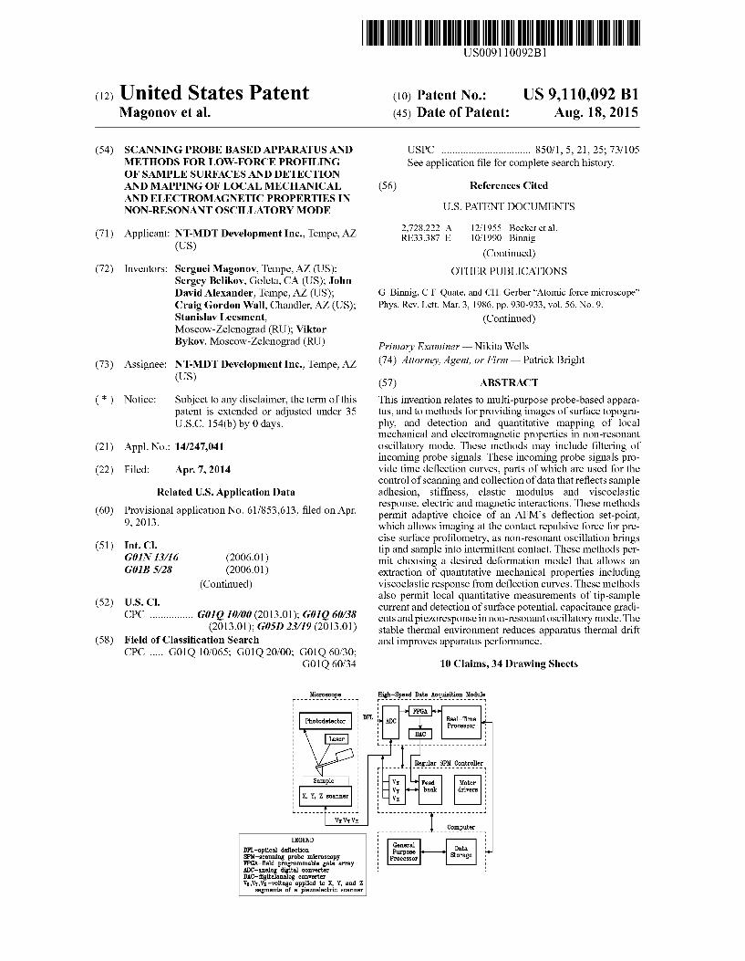
This invention relates to methods for operating probe based apparatus Such as profilometers, Scanning probe? atomic force microscopes in resonant/non-resonant oscilla tory modes, contact/non-contact/intermittent contactmodes In particular, this invention relates to AFM imaging of Sur faces in oscillatory mode, operating away from the reso nances of probe and Scanner, and to methods for recording and for quantitative on-line and off-line analysis of data related to local mechanical and electromagnetic properties of a sample. In non-resonant oscillatory mode, a vertical piezo actuator oscillates sample or probe up and down, sinusoidally, over a range of distances from a few nanometers to hundreds of nanometers so that probe tip and sample alternate between touching and non-touching states at a rate different from resonant frequencies of probe and actuator, as FIG. 1 illus trates. In response to tip-force, the probe deflects vertically, and a deflection signal is generated and recorded as shown in the electronic block diagram of a microscope, FIG. 2. FIG. 2 shows a schematic implementation of an AFM in non-reso nant oscillatory mode with a standard controller and a high speed data acquisition module. The oscillatory motion of the scanner in the vertical direction is generated by a periodic Voltage applied to the Z-segment of the scanner. Lateral ras tering/scanning results from a combination of Voltages applied to the X and Y segments of the piezo-scanner. When a sample is brought vertically into periodic contact

with the tip of a cantilevered AFM probe, the probe is deflected, and this deflection is recorded on a photodetector by a laser or super-luminescent diode beam reflected from the cantilever's surface. The related signal of the photodetector is collected by ADC in a high-speed data acquisition module, and processed in real time by FPGA (field programmable gate arrays). A deflection temporal response in non-resonant mode and a periodic Z-motion of the piezo-scanner are shown sche matically in FIG. 3. This invention relates to methods for filtering these signals and using them, with/without filtering, to control of such instruments, gentle topography profiling of samples with Such instruments, and on-line extraction of quantitative mechanical and electromagnetic properties of Such samples.

BRIEF DESCRIPTION OF THE DRAWINGS

The drawings provide examples of the methods of this invention, in which:

5

10

15

25

30

35

40

45

50

55

60

65

2 FIGS. 1A and 1B, respectively show a schematic represen

tation of atomic force microscopy (AFM), and an illustration of non-resonant oscillatory mode in AFM, where the driving frequency is Smaller than the resonant frequency of probe and actuator,

FIG. 2 is a block diagram of an AFM apparatus in non resonant oscillatory mode;

FIG.3 shows a typical temporal deflection plot, at top, and, at bottom, Z-motion of the scanner or probe;

FIG. 4 shows a flowchart with steps for filtering incoming signals, which includes filtering the D(t) signal, and, sepa rately, filtering the derivative of VZ signal and finding its Zero-crossing points, which are used for synchronization;

FIG. 5 shows down-sampling and up-sampling of AFM input signals in the real-time wavelet-based filtering;

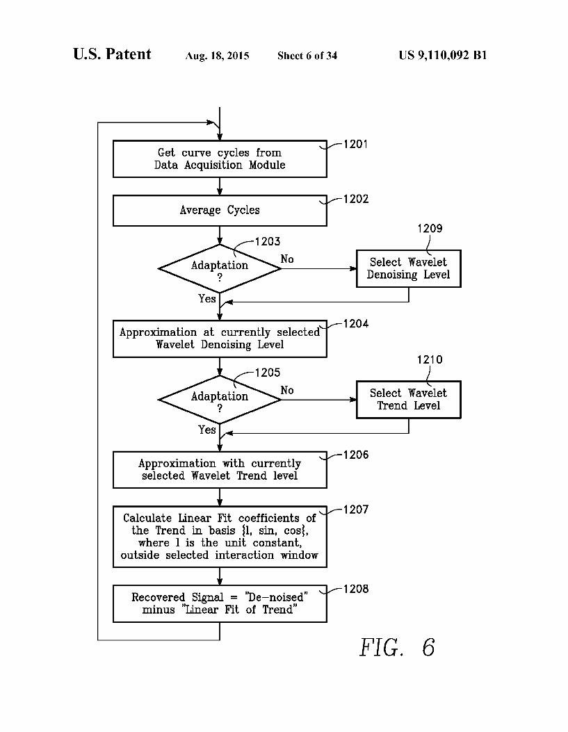
FIG. 6 shows the computer's role in real-time processing for denoising and background removal of incoming deflec tion signals using wavelet-based filtering;

FIGS. 7 and 8 show adaptive and interactive selection of appropriate wavelet levels, denoising and trend, and optimiz ing wavelet level for separating probe response curve from background;

FIGS. 9A, 9B, 9C, and 9D are illustrations of the signals obtained in the method shown in flowchart 2 that performs background removal using adaptive wavelet denoising level 4 and trend level 9 (FIG. 6), where denoising level 4 keeps details within noise bounds of the signal, and trend level 9 separates background/approximation from true curve cyclef details;

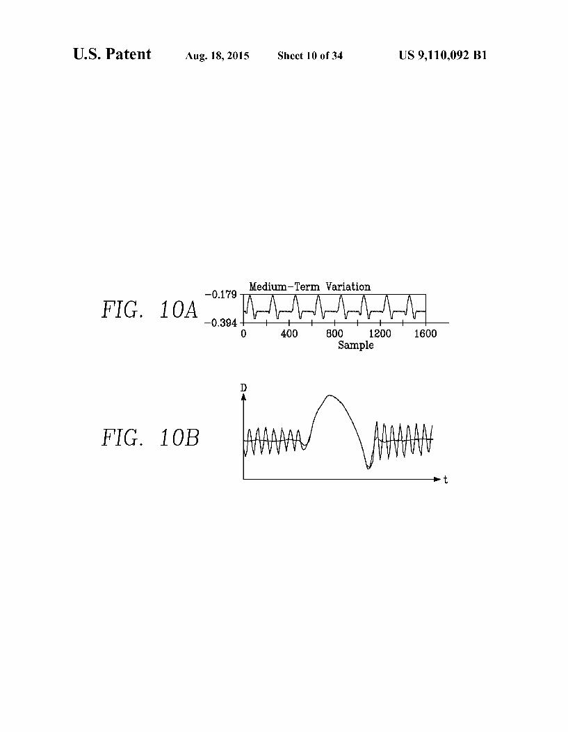
FIGS. 10A and 10B show how the FPGA method shown in FIG. 3A transforms incoming deflection signals to filtered signals using wavelet denoising level 3, including, at top, ongoing filtering during processing at FPGA:

FIGS. 11A and 11B show deflection versus time curves for a sample location with attractive tip-sample interactions (left) and without such interactions (right).

FIG. 12 shows a flowchart for deflection signal collection in a single cycle of non-resonant oscillatory mode as a sample point is moved towards a probe;

FIG.13 shows a flowchart describing imaging of all sample points at a constant set-point deflection (Dsp.) related in part to higher force contact between probe and sample;

FIGS. 14A and 14B show a desired choice of set-point deflection in DVZ curves in non-resonant oscillatory mode, and ways of determining maximum sample deformation at sample points without adhesive/attractive tip-sample interac tions, at left, and with adhesive/attractive tip-sample interac tions, at right;

FIGS. 15A, 15B, 15C, and 15D show DVZ curves may be classified into four types, depending on a sample's mechani cal response.

FIGS. 16A and 16B show two examples of DVZ curves obtained on polystyrene (PS) and polybutadiene (PBD) samples:

FIG. 17 shows a SEM micrograph of a probe with the contour of tip shape digitized, and used for tip parameteriza tion;

FIG. 18 shows a flowchart for reconstructing a DVZ curve, and assigning the curve to one of four types: elastic, elasto adhesive, viscoelastic or plastic;

FIG. 19 shows a flowchart for calculating elastic modulus of a sample from DVZ curve assigned to an elastic deforma tion case;

FIG. 20 shows a flowchart for calculating elastic modulus and work of adhesion for elasto-adhesive deformation;

FIG. 21 shows a flowchart for calculating modulus for Viscoelastic deformation.

US 9,110,092 B1 3

FIG.22 shows analysis of DVZ curves arising from plastic deformation;

FIG. 23 is a flowchart showing steps for choosing unload ing and loading traces, which are used, respectively, for modulus calculation and estimation of final plastic deforma tion h,

FIG. 24 shows a flowchart for calculating elastic modulus with plastic correction;

FIGS. 25A and 25B show the set-up for piezo-response microscopy measurements in the non-resonant oscillatory mode, and, at bottom left, probe deflection with higher fre quency overlay due to the probe response to piezo-strain in the touching part of the D(t) cycle:

FIG. 26 is a flowchart describing a measurement procedure for PFM studies in non-resonant oscillatory mode.

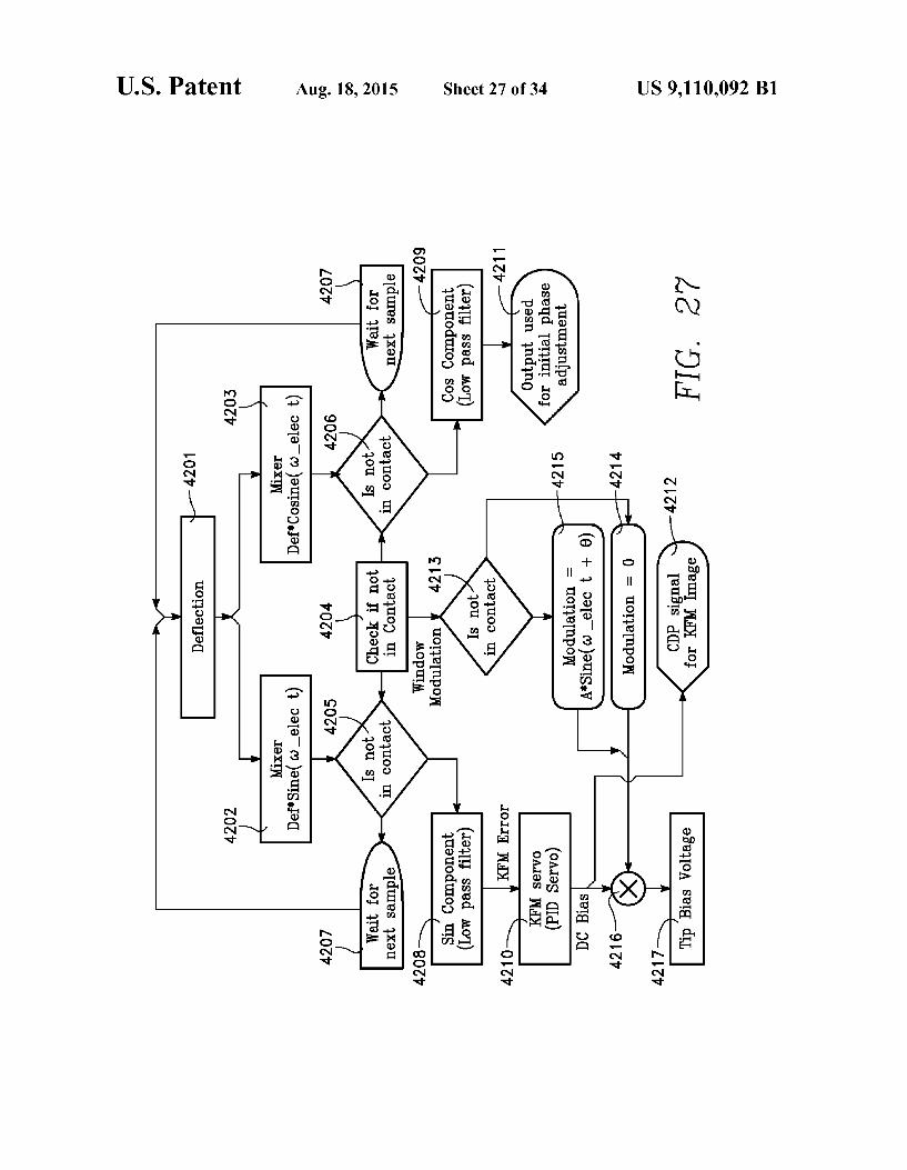
FIG. 27 is a flowchart for implementing AM-KFM tech nique in non-resonant oscillatory mode;

FIG. 28 shows that frequency of cantilever ringing after cantilever and sample separate, is affected by the electrostatic force gradient, which may be measured as a frequency shift:

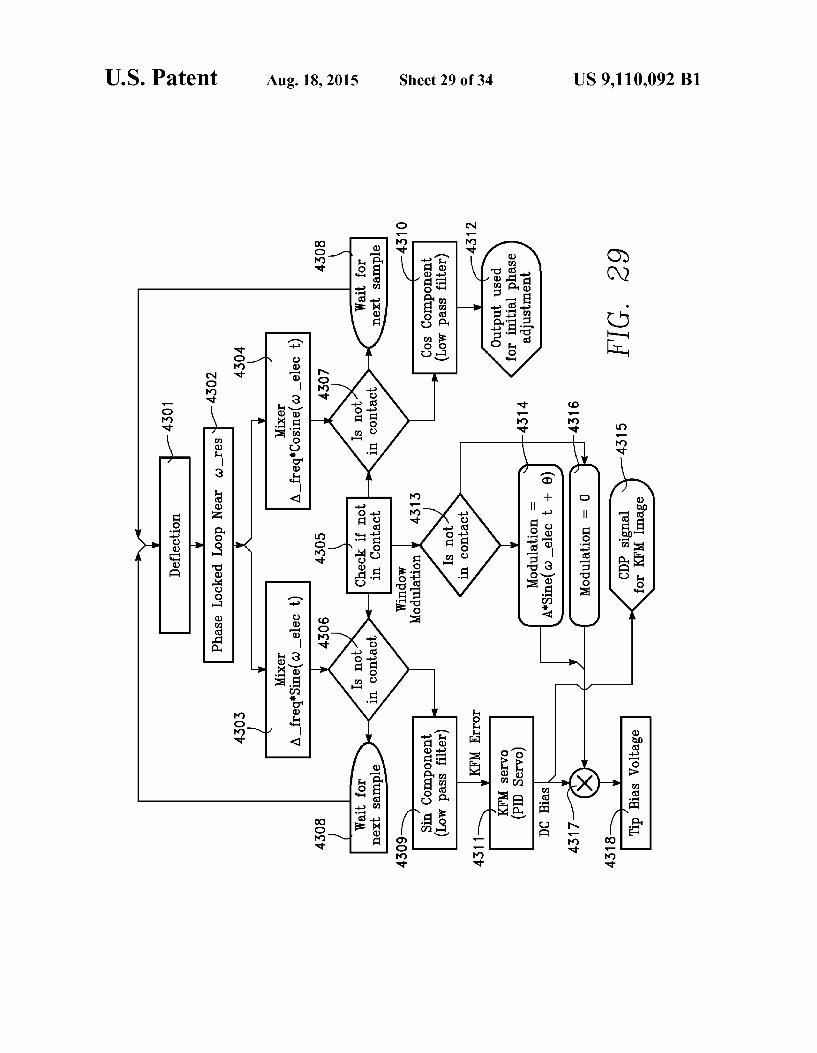
FIG. 29 is a flowchart for implementing FM-KFM opera tion in non-resonant oscillatory mode;

FIGS. 30A, 30B and 30C show an AFM cabinet with internal temperature control using convection heating and cooling:

FIG.31 is a flowchart showing automatic temperature set point adjustment;

FIG. 32 is a flowchart that describes bang-bang (In control theory, a bang-bang controller, or on-off controller, also known as a hysteresis controller, is a feedback controller that switches abruptly between two states) feedback.

DETAILED DESCRIPTION OF THE DRAWINGS

Before defining specific features of the deflection trace, which are used to extract tip-sample force interactions, and for Scanning feedback control, an incoming deflection signal from a photodetector may be filtered to counteract/remove undesirable components, such as those related to noise and artifacts, e.g., probe ringing that may arise in the non-touch ing parts of the oscillation cycle and wavy background of the whole cycle. As FIG. 2 shows, a plurality of coefficients of a filter

Suitable for removing background signal artifacts pass though a real-time processor, are calculated on the computer, and returned to FPGA. The processed signal passes to DAC, and is applied for the feedback that drives the piezo-scanner, through Voltages applied to the piezo-scanner. The feedback operation and driving of the piezo-scanner are performed with an SPM controller. An exemplary device for this purpose is the NT-MDT microscopes with HybridMode controller used as a high-speed data acquisition module. In this case, to obtain a deflection-versus-distance (DVZ) curve, which may be used for on-line and off-line quantitative nanomechanical measurements (QNM), temporal deflection signals D(t) and VZ(t), where VZ is the Voltage applied to the Z-segment of the scanner, may be synchronized (FIG. 3). Synchronizing these two signals is used to derive a DVZ curve.

The steps for acquiring incoming signals, and for filtering them, are illustrated in the flowchart of FIG.4, which includes the filtering of the D(t) signal (1101-1105), and, separately, filtering of the derivative of VZ signal and finding its zero crossing points (1106-1109), which are used for synchroni zation. Where the generation of VZ voltage and high-speed acquisition of D(t) signal are performed with a single elec tronic unit, a second branch may not be needed.

10

15

25

30

35

40

45

50

55

60

65

4 Such real-time filtering of a deflection signal, based on a

wavelet method, may remove/minimize undesirable signal noise/artifacts, may assist in recognizing signal features Such as peaks, and may also provide multi-resolution time-fre quency analysis. In real-time wavelet filtering, an incoming signal is directed into two paths. In each of these two paths, a signal undergoes high-pass and low-pass filtering, followed by down-sampling by two. In the acquisition, a signal is treated as a data sequence collected in time intervals. In the down-sampling, half of this data sequence is removed.

FIG. 5 shows, schematically, that filtering is followed by down-sampling of this data by 2 s, which is repeated 3 times for a signal diverted into the low-frequency filtering path. This down-sampling is called analysis or decomposition and the related filters are known as A-filters. The method follow ing analysis/decomposition is called synthesis or reconstruc tion. In the synthesis, also shown in FIG. 5, the up-sampling by 2s is performed 3 times, and each time it is followed by filtering with related filters, which are known as S-filters. The output signal includes the same number of components as the incoming signal. Removal of unwanted components in the high-pass or low-pass paths allows multi-resolution filtering. This method may be used in both low-frequency background removal and high-frequency ringing removal in non-resonant oscillatory mode. The flowchart in FIG. 4, which describes filtering and

finding Zero-crossing for synchronization for the probe deflection and sample Z-motion, has two branches. In the left branch of this flowchart, the initial averaging decimation from 20 MHz to 2.5 MHz (Processing speed may be higher, e.g. 5 MHz.), at block 1101, reduces signal noise, and increases the time available for the calculations. At block 1102, a Savitsky-Golay filter further reduces signal noise. This filter desirably preserves the high-frequency content of the processed signals, and the deflection curve shape. Blocks 1103 and 1104 remove intermediate parasitic signal fre quency components, which are determined by the wavelet level. Such components may include ringing signal contami nation.

In FIG.4, wavelet blocks 1103 and 1104 are followed by block 1105, where background removal from the signal, fil tered in blocks 1102, 1103, and 1105, takes place. In FPGA, removal takes place by Subtracting a linear combination of sin and cosine with coefficients pre-calculated at block 1207, as shown in Flowchart in FIG.8. The other branch of the flow chart in FIG. 4 shows that, after initial averaging down sampling of VZ signal, at block 1106, which is needed to reduce the signal noise and to increase time available for the calculations, a Savitsky-Golay Derivative filter, at block 1107, outputs a smoothed derivative of VZ signal. Block 1108 checks whether, in a particulariteration, the derivative signal changes from negative to positive, a Zero-crossing event. If not, than blocks 1101-1005 and 1106-1009 repeat. If a zero crossing is detected, the periodical cycle is complete. Block 1110 follows. The flowchart in FIG. 6 shows a computer's role in real

time processing. The computer periodically receives the available cycles containing the curves processed in controller at block 1201. At block 1202, these cycles are averaged. An averaged cycle, if no adaptation takes place at blocks 1203 and 1205, is filtered first by wavelet denoising at block 1204 to calculate “denoised signal and then by wavelet trend to calculate “trend that represents background. If adaptation is required at blocks 1203 and 1205, blocks 1209 and 1210 adaptively and/or interactively select the appropriate wavelet levels, denoising and trend, as shown in the flowcharts of FIGS. 7 and 8.

US 9,110,092 B1 5

After denoised signal and trend are calculated, the trend is fitted by {I, sine, cosine} basic functions at block 1207, where I is the unit constant. The fit is implemented outside the “force interaction window' where the background is free from the interactive curve. This allows further adjustment of back ground estimation. The fitting coefficients for {I, sine, cosine are assigned to FPGA registers to make the back ground removal, at block 1105, in FIG. 4. The “force interaction window’ can be selected interac

tively or/and adaptively as shown, for example, at block 1406 in the flowchart of FIG. 8. Recovered signal equal to the difference of the denoised signal and the fitted trend, at block 1208, is calculated for visualization and further processing, e.g. extracting mechanical properties from the AFMS response curve. The flowchart of FIG. 7 shows separation of the signal into

approximation and details parts with the optimal wavelet level. The higher the wavelet level, the greater the portion of the signal that goes to details, and the Smoother the approxi mation. The optimal is the highest level where details are within a predefined noise threshold. Block 1301 selects an initial low wavelet level. So that approximation contains most of the signal and details are within noise threshold. The details and approximation at the selected level are calculated at block 1302. If details are within the noise threshold, a higher level is tried, incrementally, at block 1302. Otherwise, as the cur rent level fails to function, the decremented level is used as selected wavelet level for denoising at block 304. The flowchart in FIG. 8 shows the process of optimizing

wavelet level for separating probe response curve from the background. This trend level must be higher than the denois ing level because background, where present, represents high amplitude-low frequency components. At block 1401, the flowchart selects denoising level from block (304) and then increments this level at block 1402 until details calculated at block 1403 reasonably represent the force curve at block 1404. Decision making at block 1404 is likewise manual or adaptive. At block 1405, this becomes the selected trend level. At block 1406, the “force interaction window' is selected, manually or adaptively.

Results illustrating wavelet filtering of background and ringing effects are shown in FIGS.9A,9B,9C,9D, 10A, and 10B. These Figures show that filtering provides contamina tion-free deflection curves.

This invention also includes methods for optimizing sample Surface profiling with probe-based apparatus. Such as AFM's and profilometers, operating in contact/intermittent contact, non-resonant modes. These methods are useful for analyzing heterogeneous samples. A feedback mechanism in non-resonant oscillatory mode maintains probe deflectionata constant level in each oscillation cycle. The choice of the set-point deflection influences defining varying-force imag ing conditions, allows gentle imaging of soft samples, and also allows examination of local mechanical sample responses, depending upon probe force on the sample. In previous implementations the set-point deflection was mea sured relative to the background deflection (deflection when the tip was not in contact with the sample). As a minimization of the repulsive force between the most advanced tip atoms and the sample is used for precise and gentle imaging of sample surfaces, the choice of the related set-point deflection depends in part on the nature of the sample/sample locations, and on the operating environment (vacuum, air, liquid). The meniscus forces in air and/or at Sticky sample points cause attractive tip-sample forces, shown as an adhesive well in deflection curves. Measuring the set-point deflection relative to the baseline in this case causes the maximum tip surface

10

15

25

30

35

40

45

50

55

60

65

6 force to increase, thus slightly distorting the Zheight, relative to sample points without these attractive forces. Minimal repulsive force may be attained when set-point level is mea sured relative to the bottom of the attractive well.

If no well is present, a minimal repulsive force is attained at a set-point near to, and just above the baseline force, as FIGS. 11A and 11B shows. For minimal repulsive tip-sample inter action the set-point should be chosen above and close to the attractive well in the case on left and above the baseline probe deflection (defined as 0-level) in the case on right.

For low-force imaging, set-point deflection should be cho Sen adaptively, at net attractive or net repulsive forces, at one or more points on a sample, through on-line adjustment of set-point deflection within the same scan. One method for recording precise sample Surface contours provides low force imaging. At each sample point, set-point deflection may be automatically chosen depending on the nature of the sample at this point. At a sticky sample point, set-point deflec tion may be near to, and slightly above the well's bottom. At a non-sticky point, the set-point may be near to, and slightly above the baseline, preferably by the same net increment as above the well's bottom. The resulting topography image reflects the vertical sample position adjustments that provide the gently-imaged Surface profile. The flowchart in FIG. 12 illustrates this method. Steps

(2101)-(2105) call for deflection signal collection in a single cycle of non-resonant oscillatory mode as a sample point is moved towards a probe. At blocks 2106 to 2108, maximal and minimal deflections, and their difference, are determined. The difference is compared with the set-point deflection at block 2109. If there is an error, the servo drives the voltage to the Z-segment of the piezo-scanner to move the sample close to the tip and the steps starting with (2101) repeat. When the error (2110) is Zero, the probe is moved to another sample point, and the method starts again with (2101).

In another method, shown in the flowchart of FIG. 13, imaging of all sample points may be performed at a constant set-point deflection (Dsp.) related in part to higher force con tact between probe and sample. In this method, the probe may deform the sample point. After the deflection versus distance (DVZ) curve is obtained (2201), it may exhibit the adhesive or snap in well, which is seen in the attractive force part of the curve. Depending on this, the starting point of the net repul sion will be determined (2203, 2204) and the single-point deformation may be calculated (2205) from the difference of deflection-versus-distance (DVZ) curve measured at this point, and DVZ curve detected on a stiff substrate (the latter measurement may be used for calculating optical sensitivity of an AFM). Consequently, the undeformed height point can be found by adding the measured height point at applied DSp and the calculated deformation value (2206).

Such measurements of sample deformation at points with different stickiness are illustrated in FIGS. 14A and 14B. These measurements can be done on line and a map of the maximal deformation can be constructed from deformation values determined at a single sample point. A Summation of height images recorded in oscillatory mode at a constant Dsp with the map of the maximal deformation may provide an accurate image of sample Surface topography.

In addition to Such on-line methods for determining accu rate maps of sample topography, these determinations may be done off-line, particularly where arrays of DVZ plots col lected at different sample points are saved, as in a data file. Such determinations may be performed using Z-vertical dis placements of the scanner that correspond to the minimal repulsive force points in the force curves, with or without adhesion of probe to sample. These off-line calculations of

US 9,110,092 B1 7

the maximal sample deformation can be used to construct deformation maps, and a Summation of deformation maps, with height data, to provide accurate Surface topography.

This invention also relates to methods for quantitative cal culations of mechanical properties of samples and the use of 5 adaptive approaches for studies of heterogeneous samples in on-line and off-line operations of probe-based instruments used for local mechanical testing. The DVZ curves and related load-versus-deformation (Pvh) curves, which are recorded either in AFM-based nanoindentation, stylus nanoindentation or in the non-resonant oscillatory AFM mode, may be applied for calculations of local mechanical properties such as elastic modulus, work of adhesion as well as viscoelasticity and plasticity responses. DVZ curves may be of four types, depending on the sam

ple's material mechanical response, as FIG. 15 shows. Pure elastic behavior is shown by DVZ curves in FIG. 15A where the loading and unloading traces coincide with each other, reflecting a complete elastic recovery of the deformation. These curves may be used for calculation of elastic modulus (E) of the sample, for example, using the elastic Hertz model.

In some cases, adhesive interaction is manifested by the attractive force wells in the loading and unloading parts of the DVZ curves as shown in FIG. 15B. Analysis of these curves may be done in the framework of elasto-adhesive solid state deformation models called DMT (Derjagin-Muller-To porov), JKR (Johnson, Kendall, Roberts) or Maugis, which provide elastic module E and work of adhesion (W). The viscoelastic material response is illustrated by the DVZ curve in FIG. 15C, in which the slopes of loading and unloading curves are different, signaling dissipative deformation. These curves also depend on time and type of loading. These curves, taken as loading or unloading traces, or as an average of these traces, are often analyzed with the above-mentioned elastic deformation models. These methods may also add calcula tions of viscoelasticity modulus.

Plastic material response is described by DVZ curves shown in FIG. 15D. Here the slopes of the loading and unloading curves are different, and the probe deflection restores its baseline deflection, the deflection level 0, prior to the point of contact in the loading cycle. The plastic response may be considered as Viscoelastic with long term deformation recovery. Analysis of plastic DVZ curves can be performed using the Sneddon integrals method with plastic correction, which allows an extraction of elastic modulus E and the plastic deformation. This approach extends the Oliver-Pharr method. Two examples of experimental DVZ curves obtained on

polystyrene (PS) and polybutadiene (PBD) samples appear in FIGS. 16A and 16B. The loading and unloading DVZ curves above the attractive wells coincide for PS and differ for PBD.

Nanomechanical analysis of DVZ curves, which are recorded in non-resonant oscillatory mode, in AFM-nanoin dentation, or in stylus nanoindentation, depends in part on the shape of the probe that deforms a sample. AFM probe shape may be described by a formula: h(r)=c(n)r", which shows dependence of tip height at radial position r with two real parameters c and n. The parameter c depends on n, which may be, but need not to be an integer. The coefficient c(n) is described by a theoretical formula for different tip shapes corresponding to n: a conical tip corresponds to n=1; a para bolic (spherical) tip to n=2; a cylindrical tip to n->OO, etc. Tips with other shapes can also be parameterized.

Tip shape affects the elastic tip-sample interaction for a probe characterized by parameters c(n) and n. The relation ship between the applied load and sample deformation may

10

15

25

30

35

40

45

50

55

60

65

8 be calculated using Sneddon integrals that for the described tip shape provide the following formula:

where P is load; h is the sample deformation; E usually unknown elastic modulus; B-calculated coefficient that depends on c(n) and n: m is calculated by the formula

m=1+1 in (3)

Table A describes the powers n and m for three different tip shapes including those mentioned above:

Interaction Shape Type Sketch l l Model

Conical N-1 1 2 Sneddon

Parabolic or N/ 2 3.2 Hertz

spherical Cylindrical ce 1 Hook

In general, probe shape may differ from those in Table A. However, ifa SEM micrograph of a probe is recorded, as seen in FIG. 17, the contour of the tip shape can be digitized,and used for tip parameterization. Tip shape is described by the formulah, c(n)r" and the coefficients c(n) for different in can be found by fitting different parts of the shape. For example, at the tip bottom, the shape can be approximated by a sphere with radius R. For this part of the shape, n=2 and coefficient c(2) can be calculated by formula c (2)=/2R. A larger part of tip shape may be considered conical with a half-angle equal to C. For this part, n=1 and c(1)=1 ?tan C. For parts between these tip portions, tip shape may vary from spherical to conical, and may be described by choosing n in the interval between 1 and 2 and finding the related c(n). The found function c(n) provide tip-shape parameterization. This process may be automated to include a large number of points on the tip. For each point, n and c(n) may be calculated by an optimal fit of the selected part of the tip shape. For interme diate n, c(n) can be interpolated. To determine on-line or off-line quantitative calculations

of sample mechanical properties, besides probe shape, one needs to know the spring constant of the probe and the optical sensitivity of the instrument, which may be determined by the measurements of the DVZ curve on a rigid Substrate Such as Sapphire or diamond. Quantitative analysis begins with filter ing and processing of D(t) and Z(t) traces, and a reconstruc tion of DVZ curve. Once the curve is obtained it should undergo a pattern recognition procedure that helps assigning the curve to one of 4 types: elastic, elasto-adhesive, viscoelas tic or plastic, see the flowchart in FIG. 18. As FIG. 18 shows, after filtering and processing of D(t) and

Z(t) signals (3101 and 3102), these signals are used to recon struct the DVZ curve (3103). This curve is analyzed for attrac tive force parts (3104). If such parts are absent, then the slopes of the repulsive parts of the loading and unloading traces are compared (3105), and the curve is assigned either to the plastic deformation case (3106) or to the elastic deformation case (3107). If the attractive parts in the DVZ are present then the slopes of the repulsive parts of the curves are compared (3108). When these slopes in the loading and unloading parts are identical, then the DVZ curve is assigned to the elasto adhesive deformation (3109). Where these slopes are differ ent, the curve is assigned to viscoelastic deformation (3110). The calculation of the elastic modulus of a sample from

DVZ curve assigned to the elastic deformation case is per formed as described by the flowchart in FIG. 19. This proce

US 9,110,092 B1 9

dure is adaptive to the parameterized tip. The chart starts by choosing either loading or unloading DVZ curve for further processing (3201). In the conversion of DVZ to Pvh (3202), the preliminary acquired data characterizing the probe spring constant (3203) and optical sensitivity, are measured from DVZ acquired on a rigid substrate (3204). Step (3205) deter mines adaptive fit of Pvh curve by the equation (2) using the tip parameterization based on its SEM micrograph (3206 3208). Block 3209 uses the theoretical relationship between mand into calculaten. At block 3210, n is used to calculate B. At block 3211, elastic modulus is obtained. The analysis of the adhesive interactions may be based on

DMT and JKR models, which are generalized and connected in Maguis approach. These models include the elastic and adhesive constituents in the load and deformation equations.

P(a) = P(E. c(n), in; a) + Pit (E. W.; a) { h(a) = heist (c(n), n; a) + hadh (E. W.; a)

For the elastic part, the Sneddon integrals applied to the parameterized tip shape with c(n) and n provide the following formulas:

P E = E 2n +1 { eas (E. c(n), n: a) = E f(c(n), n)a helast (c(n), n; a) = f3(c(n), n)a'

where f3 (n,c) is calculated by a formula derived from apply ing the Sneddon integrals to the parameterized tip. The adhe sion part depends on the selected model. As examples,

Pit (E. W: a) ={ 2it WR, DMT

W27ta WFE, JKR h(E. W. a)-. " O, DMT

The calculations of the elastic modulus and work of adhe sion for the elasto-adhesive deformation are performed as shown in the flowchart in FIG. 20. Most of the blocks (3301 3304, and 3306–3308) are parallel to those in FIG. 19. Block 3305 deals with the fitting of Pvh curves to equations used for extraction of elastic modulus and work of adhesion. When dealing with the DVZ describing the viscoelastic

behavior two approaches may be used. In the first approach, the DVZ curves, either the loading or unloading ones, or even an averaged one, may be treated with elastic or elasto-adhe sive modes, as described above. In this case the time depen dent character of Viscoelastic deformation is ignored. Esti mates of time-dependent characteristics of Viscoelastic materials, however, may ignore adhesion. For example, Such materials may be analyzed using a 3-parameter Solid model, where model initial compliance J(O) and derivative of creep compliance J'(t) are described by following formulas:

J(0) = Pl: J'(t) = A41 - dop e-li, il i041

where do, qi, p and w=do/q are known parameters of this model describing viscoelastic solids. The more common vis

10

15

25

30

35

40

45

50

55

60

65

10 coelastic complex modulus E+iE" may be calculated from these parameters by known formulas. The flowchart in FIG. 21 describes the procedure for cal

culating the complex viscoelasticity modulus. After acquir ing the temporal deflection D(t) and Z(t) signals at (3401), a time intervalt1, t2 is selected in the repulsive part of the D(t) curve (3402). At (3405), the D(t) and Z(t) signals are con verted to P(t) and h(t) using spring constant (3403) and optical sensitivity (3404) and taking into account that h(t)=Z(t)-D(t) where D(t) is converted to metric units using optical sensitiv ity. At step (3406), initial compliance J(0) and compliance derivative J'(t) are calculated with optimally fitted parameter in taken from the analysis of the tip shape in (3407)-(3409). Once known, J(O) and J'(t) may be used for calculations of the parameters of the 3-parameter solid model describing the sample viscoelasticity (3410). At step (3411) these param eters are used to calculate viscoelasticity modulus. Other Viscoelasticity models can be used instead of the 3-parameter model.

Analysis of DVZ curves arising from plastic deformation may be determined as follows. Maximal deformation (h) and final plastic deformation (h) of a sample are defined in FIG. 22, where loading and unloading traces of the plastic deformation are sketched. The flowchart in FIG. 23 describes the steps starting with a choice of the unloading and loading traces, which are used, respectively, for modulus calculation and estimation of h(3501). Conversion of the Dviz traces to Pvh curves (3502) is performed as in analysis of the elastic case with the use of the probe spring constant (3503) and optical sensitivity (3504). The steps 3505-3509 are identical to the calculations of the elastic deformation for the unload ing trace (3205-3210). Block 3510 is related to the calculation of the elastic modulus with plastic correction, which is described in detail in the flowchart in FIG. 24. This flowchart

includes the definitions of the functions (h, the adapted tip contour for the n calculated in 3509); h, and I the expres sions for Sneddon integrals for the h) used in the conse quent blocks. The calculations steps appear in blocks 3602 3605. The elastic modulus with plastic correction EP' is calculated in 3606. The DVZ curve recognition and calculations of the local

mechanical properties, which are described in the flowcharts in FIGS. 18-21 and 23–24 may be carried out in real-time or off-line. The ability to perform real-time calculations can serve as the basis of the online adaptive method in which the calculation of mechanical properties in a sample location can be performed using the model best suited for this location. These methods may be used for any probe based technique, in which the DVZ curves or similar dependencies are collected.

This invention also relates to methods of measuring tip sample electromagnetic and electro-mechanical interactions in the non-resonant oscillatory mode of operation of a probe based apparatus. When alternating between non-touching/ touching parts of an oscillatory cycle, such a probe senses mechanical interactions during touching, and also electro magnetic forces, as when conducting or ferromagnetic coat ings are applied to the probe and when a bias Voltage is applied between probe and sample. For example, electric current between the bias probe and sample can be measured in the touching part of the cycle. The probe detects these forces during touching/non-touch

ing parts of an oscillatory cycle. Such forces in non-resonant oscillatory mode appear as a change of probe baseline in response to electromagnetic or magnetic active points on a sample. Despite the demonstrated probe sensitivity to the electromagnetic forces in the non-resonant oscillatory mode, the extraction of probe responses to Such interactions and

US 9,110,092 B1 11

reduction of cross-talk between mechanical and electric effects can be achieved by measurements at specific frequen cies using lock-in amplifiers and PLL (phase-locked loop) schemes with devices that track signal changes at a particular frequency and detect frequency changes precisely. The new methods are useful in piezoresponse force micros

copy (PFM a AFM method for studies of piezo-resistive materials) and Kelvin force microscopy (KFM- an AFM method for quantitative studies of Surface potential) in non resonant oscillatory mode. PFM is a contact mode method in which changes of sample

dimensions as a function of periodically applied Voltage (electric modulation) cause piezo-electric strain to be mea Sured at the frequency of the applied Voltage. In non-resonant oscillatory mode, the probe deflection may be detected in the touching part of the D(t) cycle as shown in FIGS. 25A and 25B, showing such an instrument. When the probe leaves a sample, its deflection reflects the electrostatic force, but this signal is undesirable for evaluation of the piezoresponse. However, piezo-response may be measured with a windowed lock-in amplifier that detects the signal only in the touching part of the oscillatory cycle. Data may be obtained during a short contact window where the frequency of the electric modulation is sufficiently high to have one or more full cycles during contact time. Preferably, output low pass filters pause between contact times.

The sample motion reflecting the piezo-strain can have components in all three dimensional axes depending on the orientation of the crystal domain with respect to the tip sample electric field. Sample motion may occur in Vertical and lateral directions, and these motions may be detected by signals from different segments of the photodetector. These methods may use multiple lock-in amplifiers to detect vertical and lateral piezoresponse effects, and/or may use multiple lock-in amplifiers that are tuned to multiple frequencies if electric excitation is performed at two or more frequencies and if piezoresponse is to be recorded at the electric modula tion frequency, and at its harmonics.

The flowchart in FIG. 26 illustrates a measurement proce dure for PFM studies in non-resonant oscillatory mode. The sequence of events, in each oscillatory cycle, include obtain ing the deflection signal (4101) and sending it to the mixers (4102, 4203) where it is multiplied with sine and cosine components of the electric modulation (a periodical Voltage between the probe and the sample) at the frequency (), ). This is a standard method to measure the signed phasor mag nitude of the two orthogonal components of the deflection signal at the frequency W. Further, as contact of probe and sample is verified (4105 and 4106), signals from the mixers are directed to the low pass filters (4108 and 4109). This is a unique aspect of this lock-in demodulation, only passing the signal for calculating the two phasor magnitudes during the window when the tip is in contact. Magnitude and phase of the piezo-electric effect is calculated in (4110 and 4111). The magnitude and phase signals, which are measured at indi vidual sample points, are used to construct magnitude and phase maps, or maps of other related signals.

In KFM, local measurements of surface potential may be done by measuring electrostatic force, or its gradient, between probe and sample, which is enhanced by electric modulation. The KFM servo nullifies this signal by adding offset voltage equal to the difference of surface potentials of the probe and sample materials. In so-called amplitude modu lation KFM (AM-KFM), servo drives the DC component of the tip bias voltage to nullify the component of the deflection signal, at the modulation frequency (). In doing so the DC potential applied to the tip may equal the contact potential

10

15

25

30

35

40

45

50

55

60

65

12 difference between the tip and Surface. In non-resonant oscil latory mode, these measurements may require the frequency of electric modulation to be sufficiently high to have one or more full cycles during non-contact time. Electrostatic forces are insignificant while the tip is in contact with a sample so there is no signal to measure.

Preferably, we avoid charge transfer between tip and sample during contact. We prefer to hold the tip at the contact potential difference previously measured, so tip and sample are at the same potential, to eliminate tip-sample current, and the modulation voltage is not applied during contact. The AM-KFM procedure in non-resonant oscillatory mode, which satisfies the above-mentioned requirements, may be based on use of a windowed lock-in amplifier. The flowchart in FIG. 27 shows steps implementing AM

KFM technique in non-resonant oscillatory mode. The acquired deflection signal (42.01) is sent to mixers (4202. 4203), and there is multiplied with sine and cosine compo nents of the electric modulation at the frequency (). Fur ther, as the non-contact of the probe with a sample is verified (4204-4207) the signals from the mixers are directed to the low pass filters (4208 and 4210) and used afterwards for the KFM servo (4210) and for initial phase adjustment in (4211). From the KFM servo, the detected surface potential differ ence, or contact potential difference (CPD), is used to con struct the related image in 4212. The same signal is also applied as DC bias to the summation in 4216. Here this signal is added to the one coming from the window modulation part in 4213-4215. Here, modulation is “off” (4214) when the tip is in contact with the sample, a touching part of the oscillatory cycle, and modulation is “on” (4215) when the probe is in the non-touching part of the cycle. The summation of the modu lation signal with DC bias in 4216 provides the tip bias voltage in 4217, which brings the sample and the probe to the same potential during the contact.

In addition to AM-KFM, surface potential measurements can be attained in frequency modulation (FM) technique, which is known as FM-KFM. The difference between these methods is in use of electrostatic force gradient instead of the electrostatic force as the servo signal for nullification of the difference between surface potential of tip and sample. As FIG. 28 shows, the frequency of the ringing of the cantilever, after the cantilever separates from Sample surface, is affected by the electrostatic force gradient, which may be measured as a frequency shift. A PLL electronic scheme provides sensitive detection of frequency changes, and may be used for opera tion of FM-KFM in non-resonant oscillatory mode, as the flowchart in FIG. 29 shows. This flowchart is similar to the one describing the AM-KFM mode, but adds a PLL block 4302, which provides frequency shift to the mixers, and to the KFM servo. As with AM-KFM, window modulation avoids surface potential difference and undesired current flow during tip/sample contact in oscillatory mode. To minimize thermal drift in probe-based apparatus Such as

AFM's, and to improve signal-to-noise ratio of AFM detec tion, this invention provides athermally-stable cabinet/casing for such apparatus, in which the temperature of the AFM frame is kept constant by controlling power Supplied to a heater or cooler located inside the cabinet/casing, and by using heat convection/chimney effect to draw air over a heat exchanger to control the temperature inside the cabinet/cas 1ng.

In some embodiments, a temperature sensor is placed on the AFM instrument inside the cabinet/casing. Aheater inside the cabinet/casing raises the AFM temperature 3-4 degrees above room temperature, with a stability of -0.1 degrees when room temperature varies in the 2-3 degrees range. Alter

US 9,110,092 B1 13

natively, the AFM's temperature may be lowered with a Peltier cooler —to maintain a temperature a few degrees lower than room temperature. Alternatively, using Such heat ers and coolers together permits heating or cooling as desired/ necessary to maintain or adjust temperature inside the cabi net/casing at a desired value. Selecting average room temperature should require minimum power in this configu ration.

FIGS. 30A, 30B and 30C show an AFM cabinet with internal temperature control using convection heating, and a flowchart of cabinet operation. When heating an AFM inside the cabinet, the temperature may be kept up to 5 degrees above room temperature so that static heat from the AFM can flow out of the cabinet.

Preferably, the minimum operating temperature inside the cabinet is the difference between room temperature and AFM temperature inside the cabinet, with the AFM powered up. The temperature control servo may be abang-bang controller (In control theory, abang-bang controller (on-off controller), also known as a hysteresis controller, is a feedback controller that switches abruptly between two states) for the heating only/cooling only cabinets, or a full PID servo control. The cabinet may include one, or more than one heater/cooler and chimney. Vibration isolation may be inside or outside of the cabinet. The flowchart in FIG. 31 shows a method for recording

room temperature, and selecting/maintaining a set-point tem perature for an AFM inside a temperature-controlled cabinet by feedback control of power applied to a heater inside the cabinet. At block 5101, a user sets an initial AFM temperature inside a cabinet. At block 5102, the analog room temperature signal is detected from the room temperature sensor. At block 5103, this signal is converted to digital form, and stored in data buffer 5104. Room temperature values are collected at blocks 5103-5105 until a time for changing the set tempera ture arises at block 5106. At block 5107, recorded room temperature data is analyzed, and the maximum recorded temperature is identified at block 5108. The set-point tem perature of the AFM may be updated to a value that is the sum of the maximum temperature and a user-defined offset (5109). The flowchart in FIG. 32 describes bang-bang (In control

theory, abang-bang controller (on-off controller), also known as a hysteresis controller, is a feedback controller that switches abruptly between two states) feedback. At block 5201, AFM temperature is measured, then compared at block 5202 with set-point temperature. At block 5203, the error, denoted (Tm-Tsp), is determined. At block 5204, the error is compared with Zero. Depending on the error's value, the heater is turned offat block 5205, or turned on at block.5206. Thereafter, cycle 5201-5204 repeats. What is claimed is: 1. A method of on-line analysis of probe deflection signals

collected in non-resonant oscillatory mode of AFM or another AFM mode at a sample location, which allows deter

10

15

25

30

35

40

45

50

14 mining the deformation type of said sample, and applying to the collected signals a desired theoretical model for a defined deformation type to extract quantitative values of sample mechanical properties at said location, and repeating the col lection steps at a plurality of different locations on said sample during lateral scanning to obtain quantitative maps of mechanical properties and Surface topography in height images.

2. The method of claim 1 further comprising filtering of said signals including denoising, background removal and de-ringing.

3. The method of claim 2 further comprising wavelet fil tering with adaptive approximation and details levels in said signals.

4. The method of claim 3 further comprising real-time point-to-point implementation of wavelet-based filtering with high throughput FPGA algorithms.

5. The method of claim 3 further comprising background removal from said signals with adaptive selection of wavelet denoising levels and trend levels.

6. The method of claim 1 further comprising adaptively optimizing set-point deflection of the AFM's probe to per form imaging with minimal sample-dependent and environ ment-dependent repulsive force for determining sample Sur face topography.

7. The method of claim 6 further comprising filtering and adaptively optimizing set-point deflection of said probe to perform imaging with minimal sample-dependent and envi ronment-dependent repulsive force for determining sample Surface topography.

8. A method of measuring electric and electromechanical characteristics of a sample in non-resonant oscillatory mode ofoperation of a probe-based instrument, by applying electric modulation/a periodically varying Voltage to a probe-sample locationata frequency higher than the sample or probe oscil latory motion and detecting the probe electric or mechanical response through variations of its oscillatory parameters at or near the modulation frequency and at its harmonics in the probe/sample touching and non-touching parts of an oscilla tory cycle.

9. The method of claim 8 further comprising measuring sample piezo-response, which stimulates the sample expan sion/contraction, detected by the probe amplitude and phase changes at the modulation frequency in the touching part of the cycle, and detecting electrostatic force and force gradient variations in the non-touching part of the cycle by monitoring changes in probe oscillatory characteristics at or near modu lation frequency and its harmonics, using electric force microscopy or Kelvin force microscopy measurements.

10. The method of claim8, wherein measurements of mag netic force and gradients between a probe with ferromagnetic coating and a sample in the non-touching parts of the cycle enable magnetic force microscopy measurements in non resonant oscillatory mode.

k k k k k

Documents

(12) United States Patent (10) Patent No.: US 9,110,092 … · DFL-optical deflection : Setti Data SPM-scanning probe microscopy Processor Storage : FPGA-field programmable gate array