12 Thermal Radiation including Participating Media · · 2017-09-1312 Thermal Radiation including Participating Media Nomenclature A area ... solid angle is equal to the projected

From B. Sunden and D. Eriksson, Advanced heat and mass transfer topics

12:1

12 Thermal Radiation including Participating Media Nomenclature A area [m2] c speed of light

pc specific heat [J/(kgK)]

E emissive power [W/m2]

ijF view factor [-]

G incident radiation [W/m2] h Planck's constant [W/(m2K)] I radiative intensity [W/m2] n refractive index n unit surface normal [-] k thermal conductivity [W/(mK)] Pr Prandtl number [-] Q heat rate [W]

q heat flux [W/m2]

r position vector [m] s unit vector into a given direction [-] T temperature [K] Greek absorptivity [-] extinction coefficient

emissivity [-] wave number [1/λ]

absorption coefficient wavelength [μm] angle [rad] frequency [1/s] reflectivity [-]

Stefan Boltzmann's constant, 85.67 10 [W/m2K4]

s scattering coefficient

transmittivity [-] angular frequency [rad/s] single scattering albedo [-] angle [rad]

solid angle [sr] Subscripts b black body w wall at given wave number

at given wave length [μm]

12.1 Introduction Some of the most important engineering applications of radiative heat transfer (thermal radiation) appear in the areas of combustion of gaseous, liquid (usually in droplet form) or solid fuels. During combustion thermal radiation will carry energy directly from the combustion products to the burner walls, often at rates higher than for convection. In the cases of liquid and solid fuels, thermal radiation also plays an important role in the preheating of the fuel and its ignition. Nearly all flames are visible to the human eye and are, therefore, called luminous (sending out light). Apparently there is some radiative emission from within the flame at wavelengths where there are no vibration-rotation bands for any combustion gases. The luminous emission is known to come from tiny char particles, called soot, which are generated during the combustion process. The dirtier the flame, i.e., the higher soot content, the more luminous it is. In a combustion process, there are many intermediate chemical reactions in sequence and/or in parallel. Intermittent generation of a variety of intermediate species occurs and soot is generated, soot particles may agglomerate and subsequent partial burning of the soot may take place. Because thermal radiation contributes strongly to the heat transfer mechanism of the combustion, any understanding and modelling of the process must include knowledge of the radiation properties of the combustion gases as well as any particles being present.


12:2

In this part of the course we will give a brief general introduction to thermal radiation and then more deeply consider the so-called "equation of radiative transfer in participating media", RTE (radiative transfer equation). 12.2 Nature of thermal radiation Thermal radiative energy may be viewed as consisting of electromagnetic waves or as consisting of mass-less energy parcels, called photons. The former point of view is based on the electromagnetic wave theory while the latter one is based on quantum mechanics. However, neither of the theories is able to describe completely all radiative phenomena and, hence, it is common to use both theories interchangeably. All electromagnetic waves or photons are known to propagate through any medium at high velocity. Because light is part of the electromagnetic wave spectrum this propagation velocity is known as the speed of light denoted by c. The speed of light depends on the medium through which it travels and can be related to the speed of light in vaccum 0c , as

n

cc 0 (12.1)

where n is the refractive index of the medium. In vaccum 1n and for most gases 1n . The value of 0c is 810998.2 m/s.

A particular wave is commonly also defined by its frequency (1/s = Hz) or wavelength (commonly in m) or wave number /1 (cm-1) or angular frequency (= 2 ; radians per second). The relation between these four quantities may be written

cc

2 (12.2)

Each wave or photon carries with it an amount of energy , determined from quantum mechanics as

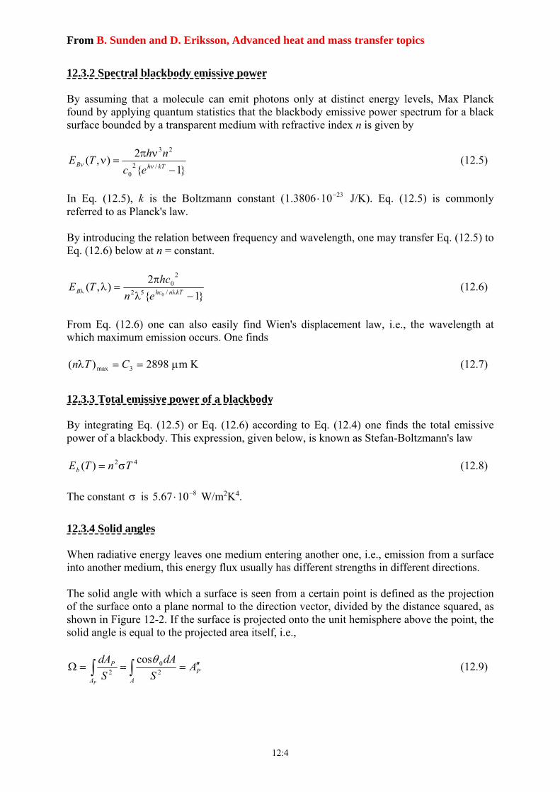
h (12.3) where h is Planck's constant. From this equation we learn that the frequency of light does not change when light penetrates from one medium to another because the energy of the photon must be conserved. However, as the refractive index is changed, the wavelength or wave number will change. Figure 12-1 shows the electromagnetic wave spectrum. Depending of the wavelength, the electromagnetic waves are grouped into different categories. Thermal radiation is usually defined to those electromagnetic waves, which are emitted by a medium due solely to its temperature. This definition limits the range of wavelengths of importance for heat transfer to between 0.1 m (ultraviolet) and 100 m (mid-infrared).


12:3

Figure 12-1. Electromagnetic wave spectrum.

12.3 Fundamental laws of thermal radiation Some introductory definitions:

If a wave passes through a medium without any attenuation, the medium is known as transparent.

If a wave is completely attenuated and no penetrating radiation occurs through the medium, the medium is known as opaque.

An opaque surface that does not reflect any radiation is called a perfect absorber or a black surface. It is also easy to show that a black surface also emits a maximum amount of radiative energy, i.e., more than any other body at the same temperature.

12.3.1 Emissive Power The radiative heat flux emitted from a surface is called the emissive power E. Usually one distinguishes between total (E) and spectral emissive power ( EE , ). Thermal radiation of a

single wavelength or frequency is called monochromatic radiation. The relation between total and spectral emissive power reads

00

),(),()( dTEdTETE (12.4)


12:4

12.3.2 Spectral blackbody emissive power By assuming that a molecule can emit photons only at distinct energy levels, Max Planck found by applying quantum statistics that the blackbody emissive power spectrum for a black surface bounded by a transparent medium with refractive index n is given by

}1{

2),(

/20

23

kThB

ec

nhTE (12.5)

In Eq. (12.5), k is the Boltzmann constant ( 23103806.1 J/K). Eq. (12.5) is commonly referred to as Planck's law. By introducing the relation between frequency and wavelength, one may transfer Eq. (12.5) to Eq. (12.6) below at n = constant.

}1{

2),(

/52

20

0

kTnhcBen

hcTE (12.6)

From Eq. (12.6) one can also easily find Wien's displacement law, i.e., the wavelength at which maximum emission occurs. One finds

2898)( 3max CTn m K (12.7)

12.3.3 Total emissive power of a blackbody By integrating Eq. (12.5) or Eq. (12.6) according to Eq. (12.4) one finds the total emissive power of a blackbody. This expression, given below, is known as Stefan-Boltzmann's law

42)( TnTEb (12.8)

The constant is 81067.5 W/m2K4.

12.3.4 Solid angles When radiative energy leaves one medium entering another one, i.e., emission from a surface into another medium, this energy flux usually has different strengths in different directions. The solid angle with which a surface is seen from a certain point is defined as the projection of the surface onto a plane normal to the direction vector, divided by the distance squared, as shown in Figure 12-2. If the surface is projected onto the unit hemisphere above the point, the solid angle is equal to the projected area itself, i.e.,

A

P

A

P AS

dA

S

dA

P

20

2

cos (12.9)


12:5

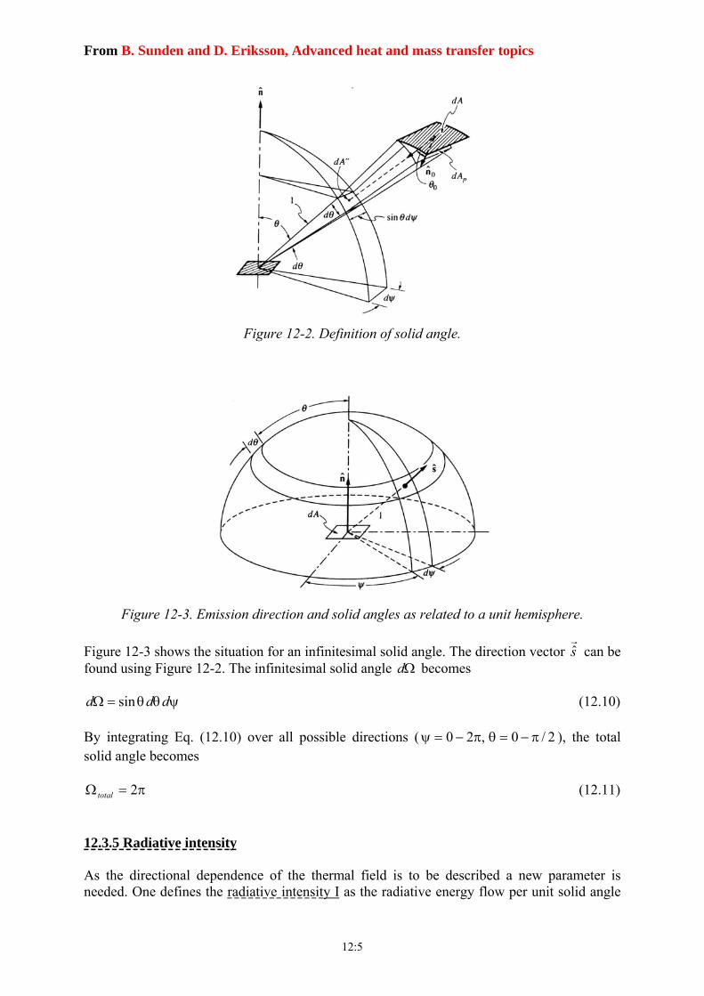
Figure 12-2. Definition of solid angle.

Figure 12-3. Emission direction and solid angles as related to a unit hemisphere.

Figure 12-3 shows the situation for an infinitesimal solid angle. The direction vector sˆ can be

found using Figure 12-2. The infinitesimal solid angle d becomes

ddd sin (12.10) By integrating Eq. (12.10) over all possible directions ( 2/0,20 ), the total solid angle becomes

2total (12.11)

12.3.5 Radiative intensity As the directional dependence of the thermal field is to be described a new parameter is needed. One defines the radiative intensity I as the radiative energy flow per unit solid angle


12:6

and unit area normal to the rays. Total as well as spectral intensities are introduced. The relation between these is written

0

ˆ ˆ( , ) ( , , )I I d

r s r s (12.12)

Here r is a position vector fixing the location in space, and s is a unit direction vector. The relation between the emissive power and the radiative intensity can be found by integrating over all directions pointing away from the considered surface.

Figure 12-4. Relationship between blackbody emissive power and intensity. By using Figure 12-4 one can find the emitted energy from surface dA in the direction s as

ˆ ˆ( , ) ( , ) cos sinPI dA d I dA d d r s r s (12.13)

Integration of Eq. (12.13) over all possible directions gives the total emitted energy from dA.

2 / 2

0 0 2

ˆ ˆ ˆ( ) ( , , ) cos sin ( , )E I d d I d

r r r s n s (12.14)

Eq. (12.14) also holds for spectral values of I and E. For a blackbody it can be shown that the intensity is independent of direction, i.e.,

),( TII bb (12.15)

From Eq. (12.14) one the finds

( , ) ( , )b bE I r r (12.16)

A surface for which the outgoing intensity is independent of direction is said to be diffuse.

n s

dAP=dAcos

dA


12:7

12.3.6 View factor or shape factor

A2

A1dA1

dA2

ndA1

ndA2S

Figure 12-5. Sketch showing area elements used in deriving the radiation view factor. To make an energy balance on a surface element the irradiation G (incident radiative heat flux) must be evaluated. In a general enclosure the irradiation will have contribution from all visible parts of the enclosure surface (or transmitting media). Therefore, one needs to determine the amount of energy which leaves one surface and reaches the other. The geometric relations governing this process are known as view factors or shape factors (sometimes angle factors). The view factor is defined as the fraction of diffuse radiation leaving a surface which reaches the other surface. Now, consider the radiative exchange between two arbitrary surfaces, see Figure 12-5. The surfaces 1dA and 2dA are infinitesimal

surfaces on the surfaces 1 and 2, respectively. The radiation leaving 1dA and reaching 2dA

moves along the line S between the centers of the surface elements. The projection of 1dA on

the lines between the centres is 11 cosdA , and the energy leaving the element 1dA in the

direction given by the angle 1 is given by

1 1 1( ) cosI dA r (12.17)

The element 2dA encompasses the solid angle d2

22 cos

S

dA (as seen from 1dA ), and the

heat transfer rate from 1dA to 2dA is then determined by

1 2

1 2 1 21 2

cos cos( )dA dA

dA dAdq I

S

r (12.18)

Integration over 1A and 2A gives the radiative energy from surface 1 to surface 2.

1 2

1 2

1 21 1 22

cos cos( )A A

A A

q I dA dAS

r (12.19)

The total radiative energy from surface 1 is 1 1 1 1 1( ) ( )Aq E A I A r r , and the view factor 12F

is the defined by

121 12 AAA qFq (12.20)


12:8

Equations (12.19) and (12.20) gives:

1 2

21221

112

coscos1

A A

dAdASA

F (12.21)

The view factor 21F (the fraction of energy leaving surface 2 and arriving at surface 1) is written as

1 2

21221

221

coscos1

A A

dAdASA

F (12.22)

From (12.21) and (12.22) one conclude, that:

212121 FAFA (12.23)

The relation (12.23) is called the law of reciprocity.

An enclosure consisting of n surfaces obeys the summation relation

1........211

niii

nj

jji FFFF (12.24)

The integration of Eq. (12.21) can be performed analytically for some simple geometries while for more complex geometries numerical integration must be used. Below view factors for some configurations are given in form of diagrams. Analytical expressions for a wide range of configurations can be found in Appendix D in Modest [1].

X/L0.1 0.5 1 5 10

0

0.05

0.1

0.15

0.2

0.25

0.3

0.150.10

0.20

0.30

0.40

0.50

0.70

1.0

2.0

Y/L =

F12

XY

L

A2

dA1

Figure 12-6. View factor 12F for a small element 1dA and a parallel rectangular surface A2 .


12:9

X/L0.1 0.5 1 5 10

0

0.1

0.2

0.3

0.4

0.5

Y/L = 0.1

0.2

0.4

0.6

1.0

1.5

2.0

4.0

6.0

10.0

20.0

F12

A1

A2

L

Y

X

Figure 12-7. View factor 12F for two rectangles with a common edge at an angle 90 to each other.

X/L0.1 1 10 100

0.01

0.05

0.1

0.5

1

Y/L = 0.1

0.2

0.3

0.4

0.6

0.81.0

1.52.0

3.05.0

10.0

F12

XY

L

A2

A1

Figure 12-8. View factor 12F between two identical parallel directly opposed rectangles.


12:10

0.1 0.5 1 5 100

0.1

0.2

0.3

0.4

0.5

0.6

0.7

0.8

0.9

1

0.4

0.5

0.6

0.8

1.0

1.25

1.5

2.0

2.53

456

8

F12

L/R1

R2

R1

A2

A1

L

Figure 12-9. View factor 12F between to parallel coaxial disk of unequal radius. 12.3.7 Radiative Heat Flux Consider the surface in Figure 12-10.

Figure 12-10. Radiative heat flux on an arbitrary surface.

Thermal radiation with an intensity ˆ( )iI s is impinging on the surface from an infinitesimal

solid angle around the direction îs . The heat flow rate per wavelength on the surface is

ˆ ˆ( ) ( ) cosi i P i i idQ I d dA I d dA s s (12.25)

The heat rate is taken as positive in the direction of the outward surface normal. Integrating over all 2 incoming directions gives

cos 0

ˆ( ) ( ) cosi

in i i iq I d

s (12.26)

R2/L = 0.3


12:11

( q unit is in W/m2/m)

The heat loss from the surface, see Figure 12-10, can be written in a similar way as

0

cos 0

ˆ( ) ( ) cosi

out o oq I d

s (12.27)

The net heat flux from the surface is found by adding equations (12.26) and (12.27)

4

ˆ( ) ( ) ( ) ( ) cosnet out inq q q I d

s (12.28)

In Eq. (12.28) the vector s is used to describe the total range of solid angle 4 . From Figure 12-10 one also finds that

ˆ ˆcos n s (12.29) As the net heat flux into the medium is evaluated as the flux into the positive n -direction, it is possible to write

4

ˆ ˆ ˆ ˆ( ) ( )netq I d

q n s n s (12.30)

Eq. (12.30) defines the radiative heat flux vector, q , that will be very important as participating media (gases, particles) are considered later. By integrating Eq. (12.30) over all the spectra one finds the total heat flux. 12.4 Radiation Characteristics of Surfaces All surfaces emit thermal radiation but at a given temperature, a black surface emits the maximum possible. To treat arbitrary surfaces a non-dimensional property called emissivity is introduced as

re temperatusame at the surfaceblack a from emittedenergy

surface a from emittedenergy (12.31)

As thermal radiation is impinging on a medium of finite thickness some of the irradiation (incoming radiation) will be reflected away from the medium, a fraction will be absorbed in the medium and the rest will be transmitted through it. The following non-dimensional properties are introduced:

Reflectivity, radiation incoming total

radiation incoming ofpart reflected (12.32)

Absorptivity, radiation incoming total

radiation incoming ofpart absorbed (12.33)


12:12

Transmissivity, radiation incoming total

radiation incoming ofpart dtransmitte (12.34)

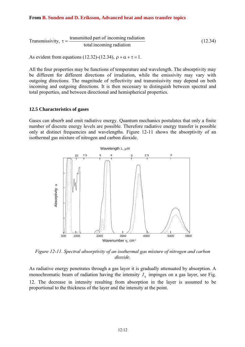
As evident from equations (12.32)-(12.34), 1 . All the four properties may be functions of temperature and wavelength. The absorptivity may be different for different directions of irradiation, while the emissivity may vary with outgoing directions. The magnitude of reflectivity and transmissivity may depend on both incoming and outgoing directions. It is then necessary to distinguish between spectral and total properties, and between directional and hemispherical properties. 12.5 Characteristics of gases Gases can absorb and emit radiative energy. Quantum mechanics postulates that only a finite number of discrete energy levels are possible. Therefore radiative energy transfer is possible only at distinct frequencies and wavelengths. Figure 12-11 shows the absorptivity of an isothermal gas mixture of nitrogen and carbon dioxide.

Wavenumber , cm-1

500 1000 2000 3000 4000 5000 5800

22.53457.510

Wavelength , m

Abs

orpt

ivity

Figure 12-11. Spectral absorptivity of an isothermal gas mixture of nitrogen and carbon dioxide.

As radiative energy penetrates through a gas layer it is gradually attenuated by absorption. A monochromatic beam of radiation having the intensity I impinges on a gas layer, see Fig.

12. The decrease in intensity resulting from absorption in the layer is assumed to be proportional to the thickness of the layer and the intensity at the point.


12:13

s ds

I

I

Figure 12-12. Absorption in a gas layer. dI I ds (12.35)

where the proportionality constant is called the monochromatic absorption coefficient.

Integrating this equation gives.

I

I

s

dsI

dI

0, 0

As indicated by the subscript the absorption coefficient depends on the wave number . It

also depends on the temperature and the pressure, (i.e., the number of receptive molecules per unit volume), and are sometimes denoted as the pressure absorption coefficient. If is

constant over the gas layer (constant pressure and temperature) the integration above becomes

0, IIs

e (12.36)

Equation (12.36) is called Beer's law and represents the familiar exponential decay formula experienced in many types of radiation analyses dealing with absorption. From the definition (12.34), the monochromatic transmissivity will be given by

s

e (12.37)

where s is the thickness of the gas layer. In the case of gases, incident radiation is either transmitted or absorbed (i.e., reflectivity 0 ), the spectral absorptivity of a gas layer is written as

1s

e 1 (12.38)

A radiating gas can be composed of molecules, atoms, ions, and free electrons that can be at various energy levels. However, the most important modes in radiative heat transfer are molecular and atom radiation. The atom or molecule moves from one quantized bound energy state to another. These states can be rotational, vibrational, or electronic in molecules and


12:14

electronic in atoms. Because bound-bound energy changes are associated with specific energy levels, the absorption and emission coefficients are sharply peak functions of frequency in the form of a series of spectral lines. The lines have a finite spectral width resulting from various line broadening mechanisms like collision broadening and Doppler broadening effects. Vibration energy modes are always coupled with rotational modes. The rotational spectral lines superimposed on a vibration line give a band of closely spaced spectral lines. If these lines overlap into a continuous region a vibration-rotation band is formed. Rotation transition, in a given vibration state, is associated with energies at long wavelengths, ~ 8-1000 μm. Vibration rotation transitions are at infrared energies of about 1.5-20 μm wavelength. There is a comprehensive database for access to line data for a certain gas or mixture of gases. This database known as HITRAN (http://cfa-www.harvard.edu/hitran//), provides line parameter information for more than 709,000 transitions at near room temperature over wavenumbers from 0 to 23,000 cm-1. These databases provide accurate quantities for performing detailed line-by-line spectral analyses with considerable numerical efforts. This kind of calculations is impractical for engineering applications but they are useful in the case of benchmark calculations, and determining the accuracy of less detailed engineering models. Various engineering models have been constructed for the line structure over a spectral interval. When this spectral interval is a portion of a complete vibration-rotation band, the model is a narrow band model. When the model covers an entire vibration-rotation band, it is a wide band model.

The three narrow band models commonly used are Elsasser model, Goody model and Malkmus model, see ref. [1]. The Elsasser model has been limited to the Lorenz line (collision broadening effect) for all lines in the band with the same half-width parameter bL. The lines within the narrow band are assumed to be overlapping, but have the same intensity Sij=Sc, have equal spacing d within the band (Figure 12-13), The absorption coefficient for the band is found by summing over all identical lines:

2 20 0

sinh 2

( ) cosh 2 cos 2 ( ) /c cL

n L

S Sb

b nd d d

(12.39)

where ( 0 ) varies between –d/2 and d/2 over each periodic line interval and /Lb d .

In the Goody model the lines are assumed to have a random distribution of wave number position within the band as shown in Figure 12-13, but have an exponential distribution of intensities. Again, all lines are assumed to have a Lorentz shape abd to have the same half-width.

Figure 12-13. Arrangement of lines for (a) Elsasser, (b) Goody or Malkmus model [1]


12:15

The Malkmus model assumes the lines have random distribution of wavenumbers within the band, and having a line intensity Sij, distribution proportional to the inverse of the intensity for low-intensity lines, and a distribution that decreases exponentially for high-intensity lines.

As mentioned, wide band models cover an entire vibration-rotation band. Exponential wide band model is one of the well-known wide band models. The method is based on the fact that absorption and emission of gases is generally concentrated within several bands and instead of considering each line, the trend of the lines in each band is approximated by an exponentially decreasing function. According to this model radiative properties are obtained by determination of three parameters, which are the integrated band intensity α, the line width to spacing parameter, β and bandwidth parameter ω. Involved expressions for calculation of α and β are in general functions of the temperature:

m

1k 0v

vu

kk

kk

m

1k vv

vu

kk

kkk

u*

0*

*

0

k

kk

k,0k

kkm

1kkk

e!v)!.1g(

)!1gv(

e!v)!.1g(

)!1gv(

e1)T(

)T(

)T()T(

(12.40)

m

1k vv

vu

kk

kkk

2m

1k vv

vu

kk

kkk

e00

0e

k,0k

kk

k,0k

kk

e!v)!.1g(

)!1gv(

e!v)!.1g(

)!1gv(

)T(

P)T(

)T(

T

TP.)T(

(12.41)

The mean intensity to spacing, S/d (which is equal to spectral absorption coefficient), can be found by one of the three simple exponential functions. Depending on band shape one has:

( ) // ( / ) uS d e (Upper limit) (12.42)

/)()/(/ ledS (Lower limit) (12.43)

2 // ( / ) cS d e (Band centre) (12.44) The band absorptance A is determined with a so-called four region expression:

HA H 1, H (12.45)

1/ 2(4 )HA H 1/, 1 (12.46)

ln( ) 2HA 1/ H , 1 (12.47)


12:16

ln 1HA H 1, 1 (12.48)

where A* =A/ is the dimensionless band absorptance and H the optical depth at the band head and can be calculated from the density path length (s is path length): X s (12.49)

H

X

(12.50)

The pressure correction factor Pe in Eq. (12.41) is calculated from:

0 0

( 1)

n

ae

PPP b

P P

(12.51)

where in this relation P0 is the atmospheric pressure, the total pressure is P and the partial pressure of the absorbing gas is Pa. The exponential wide band parameters (band centre position, b, n, 0 , 0 , and 0 ) can be found from Table 1.

Although approaches to band models have led to helpful simplifications, they are difficult to apply to non-homogeneous gases ( it is possible with scaling methods) and they can not be used at all in enclosures that have non-black walls and/or in the presence of scattering particles. In addition the wide band models suffer from less accuracy.

In order to solve these problems some new engineering models have been developed. Some of the commonly used are Weighted Sum of Grey Gas Model (WSGGM), Spectral Line Weighted Sum of Grey Gas Model (SLWSGGM), k-distribution method and correlated-k method. The interested reader can find useful materials about them in ref. [1]. 12.6 Radiation Characteristics of Particles As for a homogeneous medium, radiation travelling through a particle cloud may be transmitted, reflected or absorbed. In addition, the interaction with a particle may change the direction in which a wave travels, as indicated in Figure 12-13. This can occur by one of three different mechanisms: 1) diffraction, 2) reflection and 3) refraction in a particle (waves penetrate into the surface of particle and after partial absorption, re-emerge travelling into a different direction). The vast majority of photons are scattered elastically, and their wavelength (and energy) remain unchanged. Some parts undergo inelastic or Raman scattering (the photon re-emerges with a different wavelength) which is important in optics. In the radiative heat transfer all scattering is treated as elastic scattering. If scattering by one particle is not affected by the presence of the surrounding particles, the scattering is independent scattering otherwise the scattering is dependent.


12:17

Table 1. The wide band parameters for some gases [1].


12:18

The three mentioned phenomena in an elastic scattering together are known as scattering of radiation. The most absorption takes place as the electromagnetic wave penetrates into the particle. In the presence of scattering the equation for transmissivity is written

ss

ee s )( (12.52)

where s is the scattering coefficient and s is the extinction coefficient.

The nature of the interaction between the electromagnetic waves and particles is determined by the relative size of the particles compared with the wavelength of radiation. A particle size parameter x is defined as

a

x2

(12.53)

Figure 12-14. Interaction of electromagnetic waves with a small particle.

In 1908 Gustav Mie developed a theory based on Maxwell’s equations for a plane, monochromatic wave incident upon a homogeneous sphere in a non-absorbing medium in order to explain the colours associated with light scattering by small colloidal gold suspended in water. Solutions to the equation were later found that provided expressions for the extinction efficiency, albedo, phase function as function of only the complex index of refraction (m=n-ik) relative to the surrounding medium and the particle size parameter, x. The extinction efficiency Qe is the ratio of the extinction cross section for the particle Ce to the geometric cross section G ( 2a for a sphere). The albedo is the ratio of the scattering efficiency (or cross section) of particles to the extinction efficiency (or cross section). The phase function gives the normalized angular distribution of the intensity scattered from the particle. Except for the angular dependence of the phase function, these key properties are functions of only three parameter, namely n , k and x.

( , , ) ee

CQ n k x

G (12.54)

0 ( , , ) s

e

Qn k x

Q (12.55)

( , , , )n k x (12.56)


12:19

where e abs scaQ Q Q (12.57)

The complete solution of Mie scattering is complex and sometimes according to particle size one of these regimes (limiting solutions) can be selected: 1) 1x Rayleigh scattering 2) )1(Ox Mie scattering (for any size applicable but is recommended for this size) 3) 1x Rayleigh scattering is a limiting case when the scattering particle diameter is considerably smaller than the wavelength of the radiation. This type of scattering is important within the atmosphere, where scattering is by gas molecules. For Rayleigh scattering, the scattered energy in any direction is proportional to the inverse fourth power of the wavelength. Rayleigh scattering by molecules of the atmosphere accounts for the background of the sky being blue and for the sun appearing red at sunset. An approximative size limit for Rayleigh scattering is that the ratio of particle radius to the wavelength should be less than 0.05 or x<0.3. This is an approximation and it is considering scattering from small non-absorbing particles (sphere shapes) in a non-absorbing medium. The medium and the particle materials have subscript 1 and 2, respectively. The n is defined as the relative refractive index 2 1/n n

and the Rayleigh scattering cross section for un-polarized incident radiation is:

22 24

2

8 1,

3 4 2s

D nx

n

(12.58)

The scattering efficiency for Rayleigh scattering is:

224

2

8 1

3 1s

nQ x

n

(12.59)

and for incident un-polarized radiation, for Rayleigh scattering, the phase function is expressed as:

20 0

3( , ) (1 cos )

4 (12.60)

This phase function is independent of the circumferential angle .

Mie scattering also can be used for determination of scattering cross section, scattering efficiency and scattering phase function. Details about Mie scattering can be found in ref. [1]. When the particles are much larger than the characteristic wavelength of radiation, the simpler law of geometric optics hold even in the neighbourhood of the particle. 12.7 Radiation from luminous flame and gases Several factors complicate radiative transfer in a flame region that is actively burning. The simultaneous production and loss of energy produces a temperature variation within the flame, and thus variation of local emission and properties. Intermediate combustion products


12:20

from the complex reaction chemistry can significantly alter the radiation characteristic from those of the final products. If soot forms in burning hydrocarbons, it is a very important radiating constituent. Soot emits a continuous spectrum in the visible and infrared region and can often double or triple the radiation emitted by only the gaseous products. Soot also provides radiant absorption and emission in the spectral regions between the gas absorption bands. A method for increasing flame emission, if desired, is to promote slow initial mixing of the oxygen and fuel so that large amounts of soot form at the base of the flame. Ash particles in the combustion gases can also contribute to absorption and emission and also can significantly scatter radiation.

Calculating the effect of soot on flame radiation requires the knowledge of the soot concentration and its distribution in the flame. This is a serious obstacle for prediction of soot radiation. The soot concentration and distribution depend on the type of fuel, the mixing of fuel and oxygen, and the flame temperature. If the soot concentration and distribution can be estimated from basic equations or from observations for similar flames, another requirement for making radiative transfer calculations is the soot radiative properties. There is relatively simple empirical correlation for the absorption coefficient for as:

va

Cf

(12.61)

where fv is the soot volume fraction and C and a are empirical constants. The dispersion exponent a have been measured by investigators for many different flame conditions, ranging from as low as 0.7 to as high as 2.2.

It is possible to calculate soot absorption coefficient for small absorbing sphere from Rayleigh theory. By choosing the appropriate spectral average values for the refractive index n and absorption index k the spectral absorption coefficient is:

0vfC

(12.62)

where

0 2 2 2 2 2

36

( 2) 4

nkC

n k n k

(12.63)

12.8 Radiative Transfer Equation (RTE) (Some of the theory in this section is similar to the section above. However, some properties that was subscripted with (at a given wave number) is in this section denoted with (at a given wavelength)) In some cases it is sufficient to study the radiative heat exchange between solid surfaces without considering the medium in between the surfaces. The medium is then said to be transparent. In other cases when carbon dioxide, water vapor and particles are present, the absorption, emission and scattering of these components have to be considered. Carbon monoxide, sulphur dioxide and hydrocarbons (e.g., methane) are also good radiators but these


12:21

usually occur only in small concentrations except for combustion of biofuels. Thus they are less important. In this chapter relevant equations will be derived.

12.8.1 Absorption and scattering Consider a gas layer with thickness ds. Monochromatic radiation with intensity I is

impinging on one of the surfaces of the gas layer. As the radiation wave is travelling through the layer a part is absorbed according to

dsIdI abs )( (12.64)

where is the absorption coefficient. The negative sign indicates that the intensity is

diminishing due to the absorption. Commonly an optical thickness for absorption is introduced. This thickness is denoted by

and is defined as

s

ds0

(12.65)

The attenuation in intensity due to scattering of the incident radiation is written

dsIdI ssca )( (12.66)

where s is called the scattering coefficient.

The total attenuation of the incident radiation due to absorption and scattering is called extinction. An extinction coefficient is introduced according to

s (12.67)

A total optical depth for extinction is written as

s

ext ds0

, (12.68)

12.8.2 Augmentation due to emission and in-scattering The emitted thermal radiation within a layer of thickness ds is given by

dsIdI bem )( (12.69)

where bI is the blackbody spectral intensity.

If only emission and absorption take place the intensity follows the equation


12:22

)( II

ds

dIb (12.70)

Equation (12.70) is the radiative transfer equation in a simplified form. Let us now consider the radiation scattered into the element ds. Consider the volume element in Figure 12-15 below ( dAdsdV )

Figure 12-15. Scattered radiation for a volume element.

The radiation within the solid angle id impinging on the surface element dA is given by

ˆ ˆ ˆ( )( )i i iI dA d d s s s (12.71)

This thermal radiation travels a distance ˆ ˆ/( )ids s s through the volume element dV. The total

part being scattered is given by

ˆ ˆ ˆ ˆ( ) ( )ˆ ˆs i i i s i i

i

dsI dA d d I dAd d ds

s s s s

s s (12.72)

However, if we consider a direction s and a small solid angle d around it, only a fraction of the amount in Eq. (12.72) is scattered into this direction. To determine this fraction, the so-called scattering phase function is introduced. This function describes the probability that

a ray from one direction, îs , will be scattered into a certain direction, s

ˆ . The fraction of the

radiative energy flow within the solid angle id being scattered into the solid angle d is

written according to

ˆ ˆˆ( )

4i

s i iI dAd d ds d

s s

s (12.73)

By integrating Eq. (12.73) over all incident directions, the total in-scattered radiative energy into a solid angle d is found.

4

ˆ ˆ ˆ ˆ( ) ( ) ( , )4s i i isca

ddI dAd d I dAd d ds

s s s s

or

cross section dAds

îs

s

id d


12:23

4

ˆ ˆ ˆ ˆ( ) ( ) (s , )4

si i isca

dI ds I d

s s s (12.74)

For isotropic scattering, 1 .

12.8.3 Radiative transfer equation Let us now take an energy balance for thermal radiation propagating in a direction s . The radiative intensity is changed due to emission, absorption, scattering away from the direction s and scattering into this direction. We find

4

ˆ ˆ ˆ ˆ( , , ) ( , , ) ( , ) ( , , ) ( , , )

ˆ ˆ ˆ( ) ( ,s)4

b s b

si i i

I s ds t dt I s t I s t ds I s t ds I s t ds

I d ds

s s s s

s s

(12.75)

The left hand side may be written as

1ˆ ˆ( , , ) ( , , )I I I I

I s ds t dt I s t dt ds dst s c t s

s s (12.76)

where dtdsc / is the propagation velocity. Combining equations (12.75) and (12.76) gives

4

1 ˆ ˆ ˆ( ) ( , )4

sb s b i i i

I II I I I d

c t s

s s s (12.77)

Eq. (12.77) is the general radiative transfer equation. However, in almost all heat transfer applications the time dependence of the radiative intensity can be neglected. It should also be observed that all properties in Eq. (12.77) may vary with the position ( r

), time, wavelength

but the intensity and the phase function depend on direction. If the extinction coefficient is introduced and the derivatives of I are written as a total

derivative, and the time dependence is omitted one has

4

ˆ ˆ ˆ ˆ( ) ( , )4

sb i i i

dII I I I d

ds

s s s s (12.78)

Eq. (12.78) is generally called the radiative transfer equation (RTE).

By introducing the optical depth s

ds0

and the so-called single-scattering albedo


12:24

s

s

s (12.79)

Eq. (12.78) may be transferred to

4

ˆ ˆ ˆ(1 ) ( ) ( , )4b i i i

II I I d

s s s (12.80)

The last two terms in Eq. (12.80) are often combined and so-called source terms for the radiative intensity is introduced. The source terms is

4

ˆ ˆ ˆ ˆ( , ) (1 ) ( ) ( , )4b i i iS I I d

s s s s

Finally, the RTE can be written

ˆ( , )dI

I Sd

s (12.81)

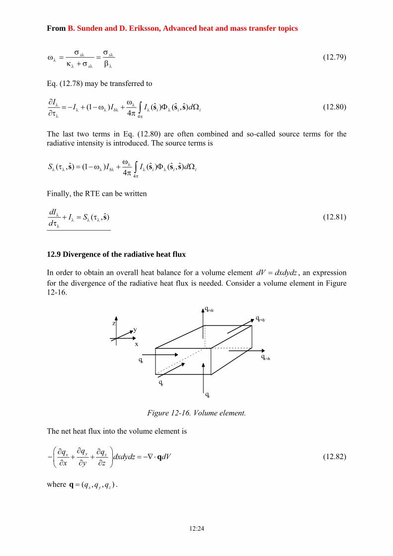
12.9 Divergence of the radiative heat flux In order to obtain an overall heat balance for a volume element dxdydzdV , an expression for the divergence of the radiative heat flux is needed. Consider a volume element in Figure 12-16.

Figure 12-16. Volume element.

The net heat flux into the volume element is

yx zqq q

dxdydz dVx y z

q (12.82)

where ( , , )x y zq q qq .

qy

qy+dy

qx+dxqx

qz

qz+dz

x

yz


12:25

Earlier an equation was given for radiation within an infinitesimal solid angle d . This was Eq. (12.78). To have a total balance for a volume element, one has to integrate over all solid angles, i.e., ]4,0[ . After rearranging the resulting equation can be written

4 4 4 4

ˆ ˆ ˆ ˆ ˆ4 ( ) ( ) ( , )4

sb i i iI d I I d I d d

s s s s s (12.83)

In this equation we recognise the radiative heat flux q as

4

Î d

q s (12.84)

The integral of the scattering phase function can readily be evaluated, i.e.,

4

ˆ ˆ( , ) 4i d

s s

Eq. (12.83) can now be written

4 4

ˆ ˆ4 ( ) ( )b s i iI I d I d

q s s (12.85)

The last two integrals concern integration over all solid angles and can be combined. If one uses s , Eq. (12.85) becomes

4

4 4b bI I d I G

q (12.86)

In Eq. (12.86) the irradians G (all incident radiation) has been introduced.

Eq. (12.86) states that the net reduction in radiative energy is equal to the difference between emitted energy and absorbed incident radiative energy. As integration has been carried out over all directions the scattering coefficient does not appear. Eq. (12.86) holds for monochromatic radiation. To obtain the overall heat flux another integration over all wavelengths is necessary. For the special case of gray medium, constant one finds

4 2 4

4

4 4T Id n T G

q (12.87)

Using optical coordinates (12.87) can be written as

2 4(1 ) 4n T G q


12:26

12.10 The complete energy equation In the general case, thermal energy is transported by heat conduction, convection and radiation. For an incompressible medium at low velocities the energy or temperature equation reads:

p

T T T Tc u v w

t x y z

q (12.88)

where

conduction radiation radiationk T q q q q (12.89)

radiationq is obtained as described in the previous sections.

12.11 Solution of the RTE, radiative transfer equation Exact solutions to Eq. (12.84) are impossible to find except for very idealized situations. The main problems are: 1. In general the geometry is complex and three dimensional.

2. Usually the temperature varies from position to position and is not known a priori. That means that the RTE has to be solved in a coupled fashion with the complete energy equation.

3. If scattering is not present, the issue is simplified considerably. If scattering is taken into account usually isotropic scattering is assumed.

4. The radiative properties are in general dependent on wavelength, pressure and temperature.

Due to the facts approximate methods have been developed. However, in this particular course we do not have time to present such methods in details but we restrict ourselves to list some of these methods with a short description. The reader is referred to the references [1], [2], [3], and [4] for further information. Many calculations presented in the literature are based on either of the methods listed below:

- Spherical harmonics method, sometimes called PN-approximation method

- Discrete Ordinates Method (DOM)

- Finite Volume Method (FVM)

- Discrete Transfer Method (DTM)

- Zonal method

- Monte Carlo method


12:27

12.11.1 The spherical harmonics method, PN-approximation method

In the general PN method the integral equation of radiative transfer is reduced to a set of differential equations by approximating the transfer relations by a finite set of moment equations. Multiplying the equation of transfer by power of the cosine of the angle between coordinate direction and the direction of the intensity, and then integration over all solid angles generates the moments. The zeroth, first, second moments at the position S are determined as:

4(0)

0

ˆ( ) ( , )I S I S d

s (12.90)

4( )

0

ˆ( ) ( , )iiI S l I S d

s (i=1,2,3) (12.91)

4( )

0

ˆ( ) ( , )iji jI S l l I S d

s (i,j=1,2,3) (12.92)

where in these equations li (i=1,2,3) is the direction cosine. These moments have a physical significance (the zeroth is the incident radiation, the first is the heat flux and the second is proportional to the local stress and pressure tensor). To develop the PN method, the intensity at each point is expressed in a series of orthogonal harmonic functions as used for solutions of the Laplacian equation in spherical coordinates:

0 1

ˆ ˆ( , ) ( ) ( )l

m ml l

l m

I I Y

r s r s (12.93)

The ( )mlI r are position dependent coefficient to be determined by the solution and ˆ( )m

lY s are

the angular dependent normalized spherical harmonics:

1/ 2

(1 )!2 1ˆ( ) exp( ) (cos ),

4 ( )!mm

l l

mlY jm P

l m

s 1j (12.94)

So exp( )jm provides the harmonics cos( )m , and sin( )m , and the last term is called associated Legendre polynomial of the first kind, of degree l and order m,

/ 222(1 )

( ) ( 1)2 !

m l mm l

l l l m

dP

l d

(12.95)

where cos 1. Values of this function are given in Table 2 for 0 3l :

1 Another definition of normalized spherical harmonics includes a factor of (-1)m. this factor introduces an alternating sign in spherical harmonics with positive m.


12:28

Table2. Associated Legendre polynomials

l m=0 m=1 m=2 m=3

0 1.0 0 0 0

1 cosθ sinθ 0 0

2 (3cos2θ-1)/2 3cosθsinθ 3sin2θ 0

3 (1/2)(5cos2θ-3)cosθ (3/2)(5cos2θ-1)sinθ 15cosθsin2θ 15sin3θ

To apply the PN method eq. (12.93) is truncated after a finite of number terms. Generally in engineering radiative transfer problems, the P1 approximation (terms are retained for l=0 and 1) or P3 approximation (terms are retained for l=0,1,2,3) is accurate enough. In numerical calculations mostly P1 approximation is used, and for an ideal form it needs some changes. In this method after some simplifications, the intensity at each point can be expressed as a function of the incident radiation and the radiative heat flux:

1ˆ ˆ( , ) ( 3 ( ) )

4I G

r s q r s (12.96)

Finally, the P1 approximation or a differential approximation for the incident radiation G can be obtained in a general form as:

1

1(4 )

3 bG I GA

(12.97)

or

1

1(1 )(4 )

3 bG I GA

This equation can be used in a gray medium with anisotropic scattering with a phase function as:

1ˆ ˆ ˆ ˆ( , ) 1 A s s s s (12.98)

For specific cases this equation is simplified. For example in a non-scattering medium one has:

2 23 (4 )bG I G (12.99)

or

2 3(4 )bG I G

In radiative equilibrium (eq. (12.87) =0, or zero radiative source term) one has:


12:29

2 2 0bG I (12.100)

The radiative heat flux can be found from:

1

1

3G

A

q (12.101)

1

1

3G

A

q

Boundary condition for P1 approximation

The usual boundary condition for diffuse wall is:

2

1( ) (1 )w w b w w iI I T l Id

(12.102)

where li is cosine angle. However, because the governing equation of the P1 approximation the right boundary condition should be in an integral form of the intensity and it requires a relation between the zeroth moment of the intensity and the wall temperature. Useful boundary conditions for engineering applications have been developed by Marshak, and these works well for the P1 approximation. Marshak boundary condition for the P1 approximation is obtained by taking the integral of the radiation intensity over the appropriate hemisphere after first multiplying by the appropriate direction cosine, as:

2 2

i i wl Id l I d

(12.103)

In order to reach an appropriate boundary condition for eq. (12.97), the eqs. (12.96) and (12.102) are substituted into eq. (12.103):

2(2 )ˆ 4w

bww

G I

n q (12.104)

Substituting eq. (12.101) into eq. (12.104) gives the final form of the boundary condition for the P1 approximation:

1

2(2 ) 1ˆ 4

(3 )w

bww s

G G IA

n (12.105)

or

1

2(2 ) 1ˆ 4

(3 )w

bww

G G IA

n


12:30

1

1(4 )

3 2(2 )w

bw wws w

GI G

A n

(12.106)

The boundary condition given by eq. (12.106) is similar to a conduction heat transfer problem with given heat flux at the boundary and can easily be incorporated as a source term of eq. (12.97). There are some methods to modify the Marshak boundary condition for the P1 approximation. For details see ref. [4].

12.11.2 The discrete ordinates method (DOM)

The DOM is a tool to transform the RTE into a set of simultaneous partial differential equations, just like the spherical harmonics method. A discrete formulation of the directional variation of the radiative intensity is the base of the DOM, and therefore DOM is simply a finite differencing of the directional dependence of the RTE. The integrals over a solid angle are approximated by numerical quadrature.

14

ˆ ˆ( ) ( )N

i ii

f d w f

s s (12.107)

where iw are the quadrature weights associated with the directions îs . The RTE, eq. (12.78),

is now written as

1

( )ˆ ˆ ˆ ˆ ˆ ˆ( , ) ( ) ( ) ( ) ( , ) ( , ) ( , , )4

Ns

i i b i j i j ij

I I I I d

rs r s r r r r s r s r s s (12.108)

Ni ,...,1

The choice of quadrature scheme is arbitrary, although restrictions on the directions and quadrature weights may arise from the desire to preserve symmetry and to satisfy certain conditions. It is customary to choose sets of directions and weights that are completely symmetric (sets that are invariant after any rotation of 90°) and that satisfy zeroth, first and second moments as:

14

4n

ii

d w

(12.109)

14

ˆ ˆ 0n

i ii

d w

s s (12.110)

14

4ˆˆ ˆ ˆ

3

n

i i ii

d w

ss s s (12.111)


12:31

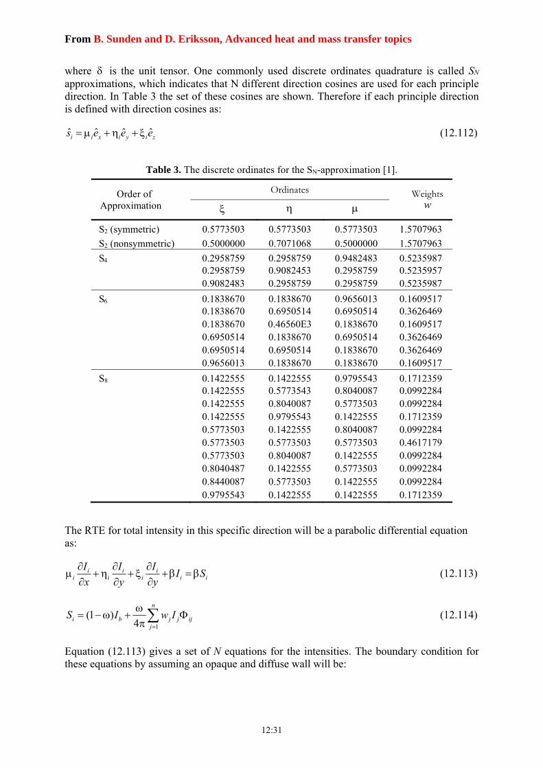
where is the unit tensor. One commonly used discrete ordinates quadrature is called SN approximations, which indicates that N different direction cosines are used for each principle direction. In Table 3 the set of these cosines are shown. Therefore if each principle direction is defined with direction cosines as: ˆ ˆ ˆ î i x i y i zs e e e (12.112)

Table 3. The discrete ordinates for the SN-approximation [1].

Order of Approximation

Ordinates Weights w

S2 (symmetric) 0.5773503 0.5773503 0.5773503 1.5707963

S2 (nonsymmetric) 0.5000000 0.7071068 0.5000000 1.5707963

S4 0.2958759 0.2958759 0.9482483 0.5235987 0.2958759 0.9082453 0.2958759 0.5235957 0.9082483 0.2958759 0.2958759 0.5235987

S6 0.1838670 0.1838670 0.9656013 0.1609517 0.1838670 0.6950514 0.6950514 0.3626469 0.1838670 0.46560E3 0.1838670 0.1609517 0.6950514 0.1838670 0.6950514 0.3626469 0.6950514 0.6950514 0.1838670 0.3626469 0.9656013 0.1838670 0.1838670 0.1609517

S8 0.1422555 0.1422555 0.9795543 0.1712359 0.1422555 0.5773543 0.8040087 0.0992284 0.1422555 0.8040087 0.5773503 0.0992284 0.1422555 0.9795543 0.1422555 0.1712359 0.5773503 0.1422555 0.8040087 0.0992284 0.5773503 0.5773503 0.5773503 0.4617179 0.5773503 0.8040087 0.1422555 0.0992284 0.8040487 0.1422555 0.5773503 0.0992284 0.8440087 0.5773503 0.1422555 0.0992284 0.9795543 0.1422555 0.1422555 0.1712359

The RTE for total intensity in this specific direction will be a parabolic differential equation as:

i i ii i i i i

I I II S

x y y

(12.113)

1

(1 )4

n

i b j j ijj

S I w I

(12.114)

Equation (12.113) gives a set of N equations for the intensities. The boundary condition for these equations by assuming an opaque and diffuse wall will be:


12:32

4

ˆ ˆ 0

1ˆ ˆ

j

wi w w w j j jI T w I

n s

n s (12.115)

The incident radiation G and radiative heat flux is given by:

14

ˆ( , ) ( )N

i ii

G I d w I

r s r

(12.116)

4

ˆ ˆ( , )I d q r s s 1

ˆ ˆ( , )N

i i ii

w I r s s

(12.117)

In two-dimensions and for a rectangular case eq. (12.113) can be solved in a general element as shown in Figure 12-17. The volume element has four face areas ,w eA A y and

,n sA A x .

Aw Ae

As

An

x

y

Pi

i

îs

Figure 12-17. Two-dimensional control volume.

The finite volume formulation is obtained by integration of eq.(12.113) over a volume element. For example the first term becomes:

, ,

exit enter

ii i i exit i enter i xe i xi i

V A A

IdV I dA I dA y I I

x

(12.118)

where Ixe,i and Ixi,i are the average intensities over the exit and enter faces. Operating similarly on the other terms changes Eq. (12.118) to:

, , , ,( ) ( ) ( )i xe i xi i i ye i yi i pi piy I I x I I V I S (12.119)

where Ipi and Spi are volume averages. The intensity at the centre of the elements can be written with a linear relation with faces intensities:

, , , ,(1 ) (1 )pi y ye i y yi i x xe i x xi iI I I I I (12.120)

This equation can be used for eliminating Ixe,i and Iye,i from eq. (12.119) which gives:


12:33

/ /

/ /pi i xi x i yi y

pii x i y

VS yI xII

V y x

(12.121)

Once Ipi has been calculated, Ixe,i and Iye,i are determined from eq. (12.120). The absolute sign is added to cover negative direction cosines. There is special method which is called the sweeping method. The calculation for each direction is started from each corner of the boundaries. The boundary condition at each surface depends on the type of surface and can be fixed. For example, for an opaque and diffuse surface eq. (12.115) can be used. In the case of

0i , the intensity at the east face of control volume is known and the intensity of the west

side must be eliminated, and for finding Ipi in this direction, from east to the west face all of control volumes should be swept. After calculating intensities in all directions and control volumes, from eq. (12.116) and eq. (12.87) the radiative heat source and from eq. (12.117) radiative heat flux can be calculated. For more details about discrete ordinates and its shortcomings see ref. [1].

12.11.3 The Finite Volume Method

The FVM is very similar to DOM and they belong to the same family. The main difference is that the FVM uses exact integration to evaluate solid angles integrals, which is analogous to the evaluation of areas and volumes in the finite volume approach. The method is fully conservative, exact satisfaction of all full-and half moments can be achieved for arbitrary geometries, and there is no loss of radiative energy. The angular grid can be adapted to each special situation. In FVM, the first step is to provide the control volume spatial discretization. So the angular space is subdivided into N N M control angles. Analogous to the

placement of the control volumes, a user has freedom to place the control angles in any desired manner. Integration of the RTE over a typical two-dimensional case gives:

( )l l

ll l l l

V V

dIdVd I S dVd

ds

(12.122)

Applying the divergence theorem, eq. (12.122) becomes:

ˆ ˆ( ) ( )l l

l l l l l l

V V

I dVd I S dVd

s n (12.123)

The left hand side of this equation presents the inflow and outflow of radiant energy across the four control volume faces. The right hand side denotes the attenuation and augmentation of energy within a control volume. With assumption of constant intensity within a control volume and control angle eq. (12.123) is simplified to:

4

1

ˆ ˆ( ) ( )l

l l l l l li i i

i

I A d I S V

s n (12.124)

By using the same approaches as in DOM, the eq. (12.124) changes to:


12:34

, , ( )

( )

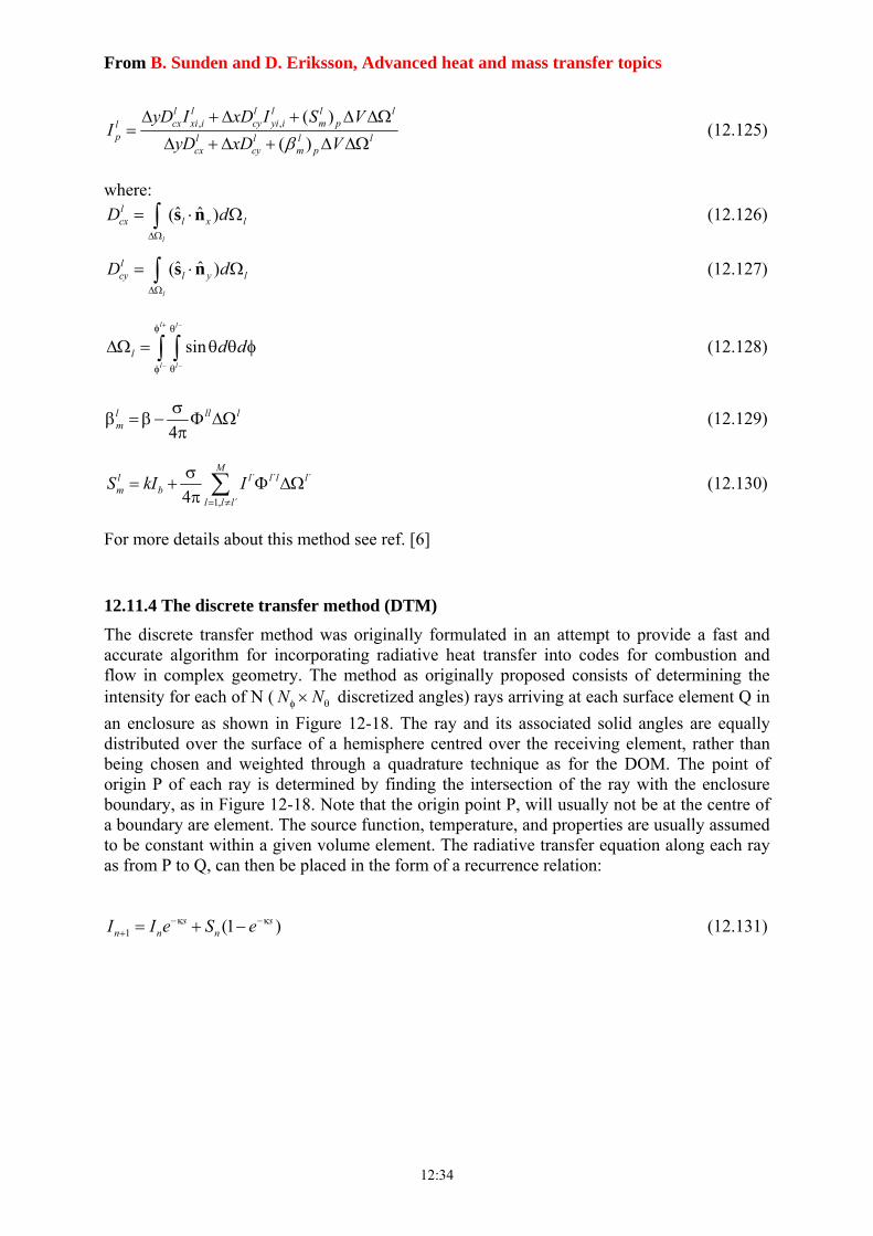
l l l l l lcx xi i cy yi i m pl

p l l l lcx cy m p

yD I xD I S VI

yD xD V

(12.125)

where:

ˆ ˆ( )l

lcx l x lD d

s n (12.126)

ˆ ˆ( )l

lcy l y lD d

s n (12.127)

sin

l l

l l

l d d

(12.128)

4l ll lm

(12.129)

´ ´ ´

1, ´4

Ml l l l lm b

l l l

S kI I

(12.130)

For more details about this method see ref. [6]

12.11.4 The discrete transfer method (DTM)

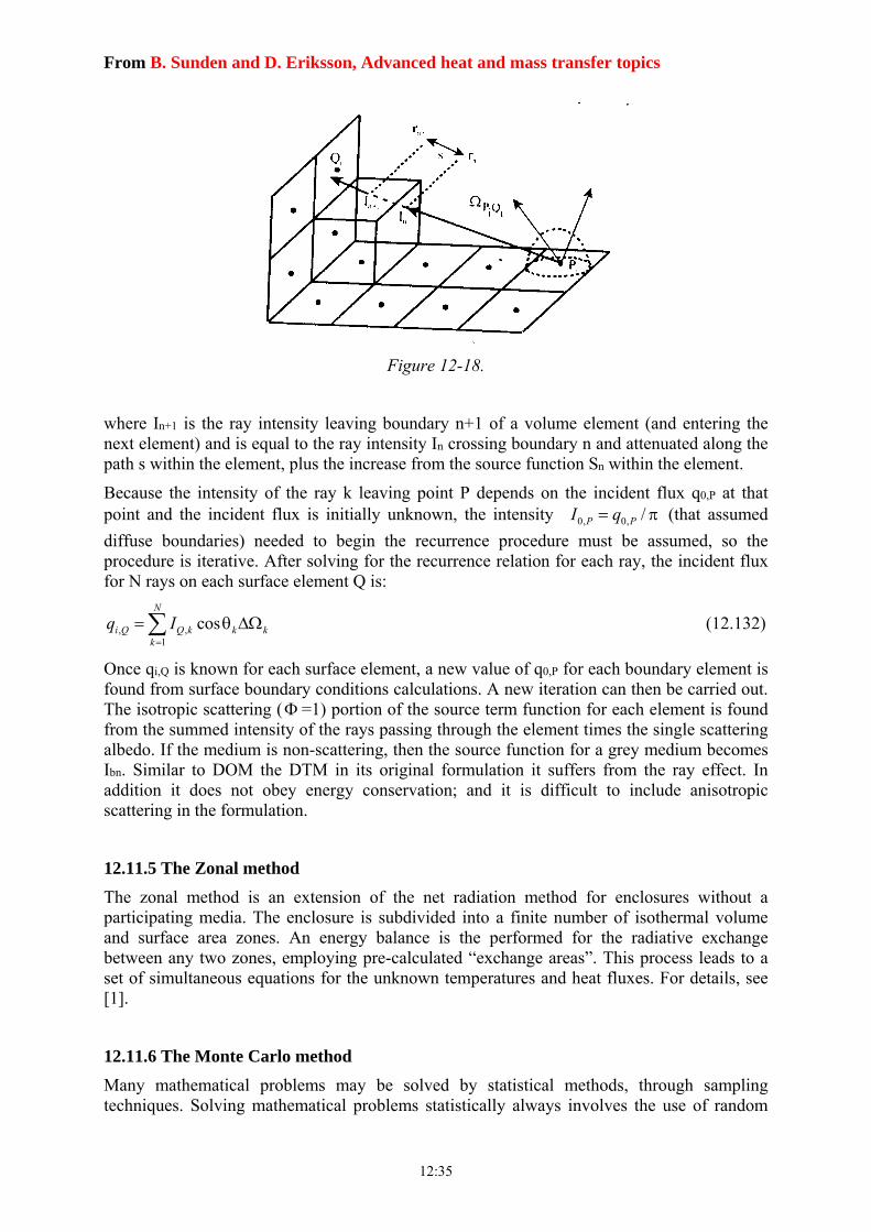
The discrete transfer method was originally formulated in an attempt to provide a fast and accurate algorithm for incorporating radiative heat transfer into codes for combustion and flow in complex geometry. The method as originally proposed consists of determining the intensity for each of N ( N N discretized angles) rays arriving at each surface element Q in

an enclosure as shown in Figure 12-18. The ray and its associated solid angles are equally distributed over the surface of a hemisphere centred over the receiving element, rather than being chosen and weighted through a quadrature technique as for the DOM. The point of origin P of each ray is determined by finding the intersection of the ray with the enclosure boundary, as in Figure 12-18. Note that the origin point P, will usually not be at the centre of a boundary are element. The source function, temperature, and properties are usually assumed to be constant within a given volume element. The radiative transfer equation along each ray as from P to Q, can then be placed in the form of a recurrence relation:

1 (1 )s sn n nI I e S e (12.131)


12:35

Figure 12-18.

where In+1 is the ray intensity leaving boundary n+1 of a volume element (and entering the next element) and is equal to the ray intensity In crossing boundary n and attenuated along the path s within the element, plus the increase from the source function Sn within the element.

Because the intensity of the ray k leaving point P depends on the incident flux q0,P at that point and the incident flux is initially unknown, the intensity 0, 0, /P PI q (that assumed

diffuse boundaries) needed to begin the recurrence procedure must be assumed, so the procedure is iterative. After solving for the recurrence relation for each ray, the incident flux for N rays on each surface element Q is:

, ,1

cosN

i Q Q k k kk

q I

(12.132)

Once qi,Q is known for each surface element, a new value of q0,P for each boundary element is found from surface boundary conditions calculations. A new iteration can then be carried out. The isotropic scattering ( =1) portion of the source term function for each element is found from the summed intensity of the rays passing through the element times the single scattering albedo. If the medium is non-scattering, then the source function for a grey medium becomes Ibn. Similar to DOM the DTM in its original formulation it suffers from the ray effect. In addition it does not obey energy conservation; and it is difficult to include anisotropic scattering in the formulation.

12.11.5 The Zonal method

The zonal method is an extension of the net radiation method for enclosures without a participating media. The enclosure is subdivided into a finite number of isothermal volume and surface area zones. An energy balance is the performed for the radiative exchange between any two zones, employing pre-calculated “exchange areas”. This process leads to a set of simultaneous equations for the unknown temperatures and heat fluxes. For details, see [1].

12.11.6 The Monte Carlo method

Many mathematical problems may be solved by statistical methods, through sampling techniques. Solving mathematical problems statistically always involves the use of random


12:36

number, e.g., by placing a ball into a spinning roulette wheel. For this reason sampling methods are called Monte Carlo methods. There is no single scheme to which the name Monte Carlo applies. Rather, any method with an appropriate statistical sampling technique is commonly referred to as a Monte Carlo method.

Radiative energy travels in discrete parcels (photons) over relatively long distances along a straight path before interaction with matter. Thus, solving a thermal radiation problem by Monte Carlo implies tracing of the history of a statistically meaningful random sample of photons from their points of emission to their points of absorption. For details see ref. [7]

12.7 How to choose a radiation model The choice of an appropriate radiative transfer model is important. The radiative transfer model is coupled with models for flow, chemical kinetics, turbulence, and so on, so it is favourable to choose a model that will be compatible with the solution techniques for the other governing equations. The model should also be reliable, computationally efficient, and able to predict accurately the radiative flux and the divergence of radiative flux distributions in the medium. It is not always necessary to choose the most accurate radiative transfer model, if the accuracy of the radiative property data used in predictions is not as good as the accuracy of the model itself. A coarse picture of the problem will help the selection of an appropriate model. It is favourable to know how simple/complex the medium geometry is, if there are steep temperature and species concentration distributions in the medium, if there are anisotropically scattering particles (and what kind of scattering phase function approximations can be used for them), before a specific model is chosen. No model can be used on a universal basis for the solution of the RTE, so several different models are available. To name a few, we have: numerical methods (e.g., FVM), Rosseland-approximation, the zone method, the Monte Carlo method, flux models (e.g., DTM and DOM), and moment methods (to which the P1-approximation belongs). The advantages, disadvantages, range of applicability, and versatility of each model can be found in Table 4. The RTE, a complicated integro-differential equation of a physical model, i.e., the conservation of the radiative energy, is written in terms of radiation intensity, which is a function of seven (x, y, z, t, , , ) independent parameters. There is no available analytical solution to the RTE in its general form, so physical and/or mathematical approximations are to be introduced. Different categories of approximations are possible, e.g., simplification of the spectral nature of properties, angular discretisation of the intensity field, and spatial discretisation of the medium (for all parameters). The divergence of the radiative flux enters into the energy equation as a source term, so the solution of the RTE is required only to obtain the divergence of the radiative flux vector (a spectrally integrated quantity). Because a spectrally integrated quantity is needed, one way to simplify the problem, is by using spectrally averaged radiative properties. As the medium must be discretised spatially to perform the numerical calculations, the same discretisation for radiative transfer calculations as for flow and other scalar field calculations should be used. In this work total radiative properties have been used, and the same grid has been utilised for all properties. The radiative flux is an integrated quantity over an angular domain, and as such, it could be


12:37

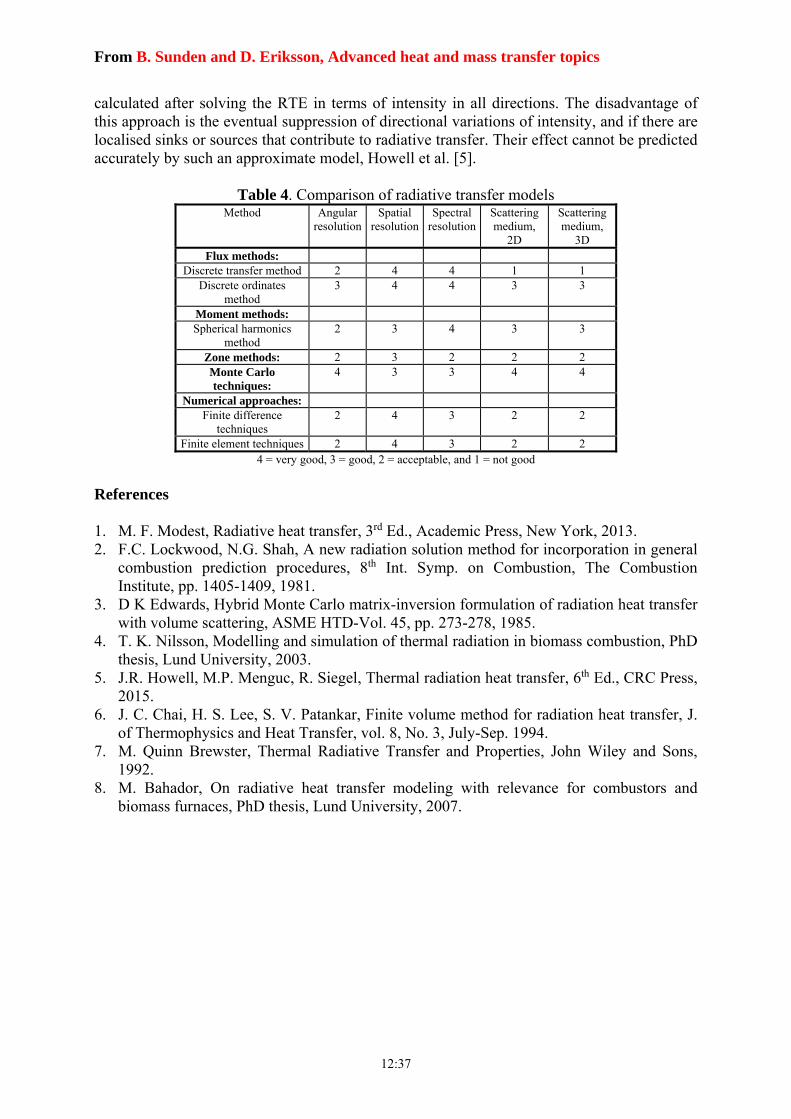
calculated after solving the RTE in terms of intensity in all directions. The disadvantage of this approach is the eventual suppression of directional variations of intensity, and if there are localised sinks or sources that contribute to radiative transfer. Their effect cannot be predicted accurately by such an approximate model, Howell et al. [5].

Table 4. Comparison of radiative transfer models Method Angular

resolutionSpatial

resolutionSpectral

resolutionScattering medium,

2D

Scattering medium,

3D Flux methods:

Discrete transfer method 2 4 4 1 1 Discrete ordinates

method 3 4 4 3 3

Moment methods: Spherical harmonics

method 2 3 4 3 3

Zone methods: 2 3 2 2 2 Monte Carlo techniques:

4 3 3 4 4

Numerical approaches: Finite difference

techniques 2 4 3 2 2

Finite element techniques 2 4 3 2 2 4 = very good, 3 = good, 2 = acceptable, and 1 = not good

References 1. M. F. Modest, Radiative heat transfer, 3rd Ed., Academic Press, New York, 2013. 2. F.C. Lockwood, N.G. Shah, A new radiation solution method for incorporation in general

combustion prediction procedures, 8th Int. Symp. on Combustion, The Combustion Institute, pp. 1405-1409, 1981.

3. D K Edwards, Hybrid Monte Carlo matrix-inversion formulation of radiation heat transfer with volume scattering, ASME HTD-Vol. 45, pp. 273-278, 1985.

4. T. K. Nilsson, Modelling and simulation of thermal radiation in biomass combustion, PhD thesis, Lund University, 2003.

5. J.R. Howell, M.P. Menguc, R. Siegel, Thermal radiation heat transfer, 6th Ed., CRC Press, 2015.

6. J. C. Chai, H. S. Lee, S. V. Patankar, Finite volume method for radiation heat transfer, J. of Thermophysics and Heat Transfer, vol. 8, No. 3, July-Sep. 1994.

7. M. Quinn Brewster, Thermal Radiative Transfer and Properties, John Wiley and Sons, 1992.

8. M. Bahador, On radiative heat transfer modeling with relevance for combustors and biomass furnaces, PhD thesis, Lund University, 2007.


12:39

Documents

12 Thermal Radiation including Participating Media · · 2017-09-1312 Thermal Radiation including Participating Media Nomenclature A area ... solid angle is equal to the projected