DesignCon 2007

EMI Emissions from Mismatches in High Speed Differential Signal Traces and Cables Bruce Archambeault, IBM, Research Triangle Park, NC barch@us.ibm.com Joseph C. (Jay) Diepenbrock, IBM, Research Triangle Park, NC jaydiep@us.ibm.com Samuel Connor, IBM, Research Triangle Park, NC sconnor@us.ibm.com

Abstract The use of so-called differential signaling for high speed signals has become very common in today’s high speed system designs. While this signal strategy allows better data quality and signal integrity at the receive end of the traces and/or cables, there are some significant EMC and signal integrity issues that are not readily apparent. This paper demonstrates that a significant amount of common-mode current can be created when the two legs of the differential signal are skewed in time, or if the rise/fall times differ. These common mode currents can impact the EMC performance, causing significant levels of emissions unless careful design consideration is given to common-mode (ground) current return. Author(s) Biography Bruce Archambeault (M ’85, SM ’99, F ’05) is an IBM Distinguished Engineer at IBM in Research Triangle Park, NC. He received his B.S.E.E degree from the University of New Hampshire in 1977 and his M.S.E.E degree from Northeastern University in 1981. He received his Ph. D. from the University of New Hampshire in 1997. His doctoral research was in the area of computational electromagnetics applied to real-world EMC problems.

Dr. Archambeault has authored or co-authored a number of papers in computational electromagnetics, mostly applied to real-world EMC applications. He is currently a member of the Board of Directors for the IEEE EMC Society and a past Board of Directors member for the Applied Computational Electromagnetics Society (ACES). He has served as a past IEEE/EMCS Distinguished Lecturer. He is the author of the book “PCB Design for Real-World EMI Control” and the lead author of the book titled “EMI/EMC Computational Modeling Handbook”. Joseph C. (Jay) Diepenbrock received the Sc. B. and M. S. degrees in electrical engineering from Brown University, Providence, RI, and Syracuse University, Syracuse, NY, in 1976 and 1983, respectively. Mr. Diepenbrock has been with IBM since 1976, and has worked in a number of areas including bipolar and CMOS IC design, analog and digital circuit design, backplane design and simulation, and network hardware and server product development. He is currently a Senior Technical Staff Member in the Interconnect Qualification Engineering department in IBM’s Integrated Supply Chain organization, working on the electrical testing and modeling of connectors and cables. This work involves hardware testing and software simulation of various interconnect structures, lossy model generation and verification, and development of electrical test procedures and software. Mr. Diepenbrock has authored papers at various IEEE and other conferences, contributed to a number of industry standards including USB, EIA 364 electrical test methods, and PCI Express specifications, and is currently leading the Cable/Connector subteam of the Electromechanical Working Group of the InfiniBand

Trade Association. He has received two European and six US patents, with others pending. Sam Connor (M '05) received his BSEE from the University of Notre Dame in 1994. He currently works at IBM in Research Triangle Park, NC, where he is a senior engineer responsible for the development of EMC and SI analysis tools/applications. Mr. Connor has co-authored several papers in computational electromagnetics, mostly applied to decoupling and high-speed signaling issues in PCB designs.

Introduction The use of so-called differential signaling for high speed signals has become very common in today’s high speed system designs. While this signal strategy allows better data quality and signal integrity at the receive end of the traces and/or cables, there are some significant EMC and signal integrity issues that are not readily apparent. This paper demonstrates that a significant amount of common-mode current can be created when the rise/fall times of the differential signals have small amounts of skew, or if the rise/fall times are slightly different. These common mode currents can have a significant impact on the EMC performance, causing significant levels of emissions unless careful design consideration is given to common-mode current return (ground return). Small amounts of common mode signals can have significant impact on the printed circuit board’s and system level EMC performance. The common mode signals can occur due to three primary causes: (1) skew between the two signals making up the pseudo-differential pair due to unequal delay in either the ASIC drivers or signal paths (card traces or cable), (2) differing rise/fall times from the ASIC drivers, and (3) differential to common mode conversion in connectors, vias, etc. Many differential signal drivers in today’s high speed system designs actually use a pair of complementary single-ended drivers (once the actual drivers are analyzed in the driving ASIC). That is, both traces are driven out of phase with respect to the PCB ground-reference. For this reason, we call these nets “pseudo-differential,” while true differential signaling would drive the two signals symmetrically around a ground reference. At the receive end, the ASIC is usually a true differential receiver which only looks for the difference between the two nets, without reference to the PCB ground-reference plane. In this way, the complementary single-ended nets become differential at the receiver. Since the receiver is only measuring the difference between the two nets, any common mode signals (signals that exist on both nets at the same time and in phase) are ignored by the receiver. This provides additional signal quality and allows longer traces to be used for higher data rates than the traditional single-ended nets since much of the incident noise is coupled equally to both legs of the differential pair. From an EMC perspective, the common mode signals on these traces and cables can cause the same problems as any single-ended trace/cable. In fact, common mode currents cause these traces and cables to be equivalent to high speed single-ended nets from the common mode signal point of view. In addition to common mode currents caused by skew and/or rise/fall time mismatch in the drivers, common mode currents can be created by differential trace length mismatch, and by cable in-pair skew. Measured data will be presented to show that significant amounts of common mode signals can be created in cables, resulting in higher than expected cable shielding requirements to prevent excessive radiation. Effects of Skew An example pseudo-differential signal of 1 Gb/s (500 psec pulse width) with a nominal rise/fall time of 95 ps was created using a spreadsheet program. The second output of the

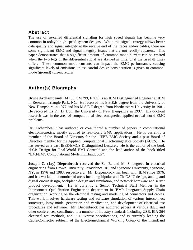
complementary driver was delayed, introducing skew from two to 60 ps. This skew represents a skew of 0.4% to 12% of the pulse width. The resulting voltage waveforms are shown in Figure1.

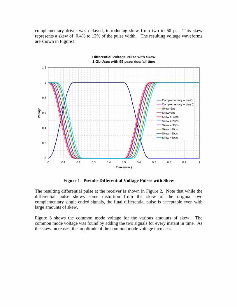
Figure 1 Pseudo-Differential Voltage Pulses with Skew The resulting differential pulse at the receiver is shown in Figure 2. Note that while the differential pulse shows some distortion from the skew of the original two complementary single-ended signals, the final differential pulse is acceptable even with large amounts of skew. Figure 3 shows the common mode voltage for the various amounts of skew. The common mode voltage was found by adding the two signals for every instant in time. As the skew increases, the amplitude of the common mode voltage increases.

Differential Voltage Pulse with Skew1 Gbit/sec with 95 psec rise/fall time

0

0.2

0.4

0.6

0.8

1

1.2

0 0.1 0.2 0.3 0.4 0.5 0.6 0.7 0.8 0.9 1

Time (nsec)

Volta

ge

Complementary -- Line1Complementary -- Line 2Skew=2psSkew=6psSkew = 10psSkew = 20psSkew = 30psSkew =40psSkew =50psSkew =60ps

Figure 2 Differential Voltage Pulse Shape

Figure 3 Skew-induced Common Mode Voltage

Resulting Differential Voltage Pulse with Skew1 Gbit/sec with 95 psec rise/fall time

-1.5

-1

-0.5

0

0.5

1

1.5

0 0.1 0.2 0.3 0.4 0.5 0.6 0.7 0.8 0.9 1

Time (nsec)

Volta

ge

BalancedSkew=2psSkew=6psSkew =10psSkew =20psSkew =30psSkew =40psSkew =50psSkew =60ps

Common Mode VoltageFrom Differential Voltage Pulse with Skew

1 Gbit/sec with 95 psec rise/fall time

-0.6

-0.4

-0.2

0

0.2

0.4

0.6

0 0.1 0.2 0.3 0.4 0.5 0.6 0.7 0.8 0.9 1

Time (nsec)

Volta

ge

BalancedSkew=2psSkew=6psSkew =10psSkew =20psSkew =30psSkew =40psSkew =50ps

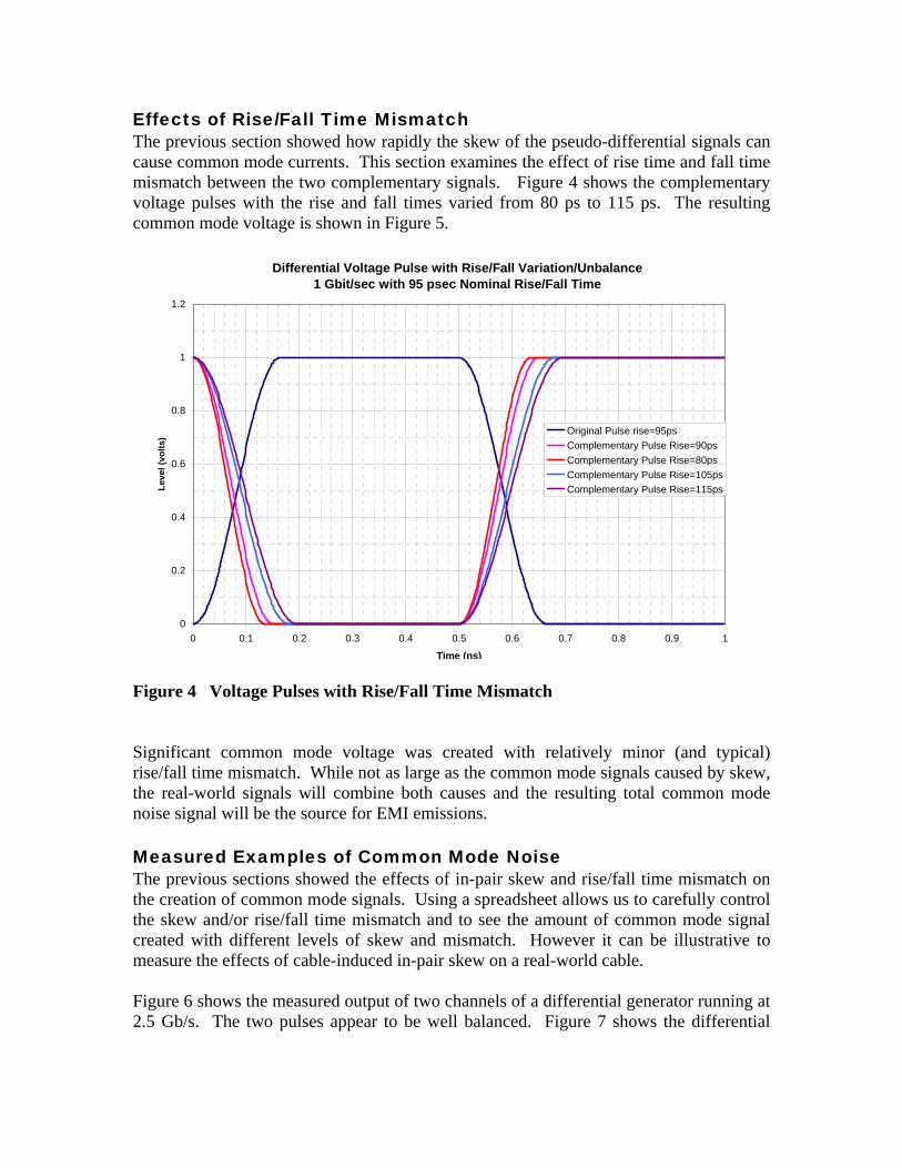
Effects of Rise/Fall Time Mismatch The previous section showed how rapidly the skew of the pseudo-differential signals can cause common mode currents. This section examines the effect of rise time and fall time mismatch between the two complementary signals. Figure 4 shows the complementary voltage pulses with the rise and fall times varied from 80 ps to 115 ps. The resulting common mode voltage is shown in Figure 5. Figure 4 Voltage Pulses with Rise/Fall Time Mismatch Significant common mode voltage was created with relatively minor (and typical) rise/fall time mismatch. While not as large as the common mode signals caused by skew, the real-world signals will combine both causes and the resulting total common mode noise signal will be the source for EMI emissions. Measured Examples of Common Mode Noise The previous sections showed the effects of in-pair skew and rise/fall time mismatch on the creation of common mode signals. Using a spreadsheet allows us to carefully control the skew and/or rise/fall time mismatch and to see the amount of common mode signal created with different levels of skew and mismatch. However it can be illustrative to measure the effects of cable-induced in-pair skew on a real-world cable. Figure 6 shows the measured output of two channels of a differential generator running at 2.5 Gb/s. The two pulses appear to be well balanced. Figure 7 shows the differential

Differential Voltage Pulse with Rise/Fall Variation/Unbalance1 Gbit/sec with 95 psec Nominal Rise/Fall Time

0

0.2

0.4

0.6

0.8

1

1.2

0 0.1 0.2 0.3 0.4 0.5 0.6 0.7 0.8 0.9 1

Time (ns)

Leve

l (vo

lts) Original Pulse rise=95ps

Complementary Pulse Rise=90psComplementary Pulse Rise=80psComplementary Pulse Rise=105psComplementary Pulse Rise=115ps

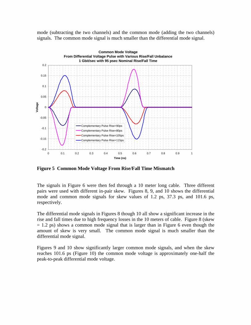
mode (subtracting the two channels) and the common mode (adding the two channels) signals. The common mode signal is much smaller than the differential mode signal. Figure 5 Common Mode Voltage From Rise/Fall Time Mismatch The signals in Figure 6 were then fed through a 10 meter long cable. Three different pairs were used with different in-pair skew. Figures 8, 9, and 10 shows the differential mode and common mode signals for skew values of 1.2 ps, 37.3 ps, and 101.6 ps, respectively. The differential mode signals in Figures 8 though 10 all show a significant increase in the rise and fall times due to high frequency losses in the 10 meters of cable. Figure 8 (skew = 1.2 ps) shows a common mode signal that is larger than in Figure 6 even though the amount of skew is very small. The common mode signal is much smaller than the differential mode signal. Figures 9 and 10 show significantly larger common mode signals, and when the skew reaches 101.6 ps (Figure 10) the common mode voltage is approximately one-half the peak-to-peak differential mode voltage.

Common Mode VoltageFrom Differential Voltage Pulse with Various Rise/Fall Unbalance

1 Gbit/sec with 95 psec Nominal Rise/Fall Time

-0.2

-0.15

-0.1

-0.05

0

0.05

0.1

0.15

0.2

0 0.1 0.2 0.3 0.4 0.5 0.6 0.7 0.8 0.9 1

Time (ns)

Volta

ge

Complementary Pulse Rise=90ps

Complementary Pulse Rise=80ps

Complementary Pulse Rise=105ps

Complementary Pulse Rise=115ps

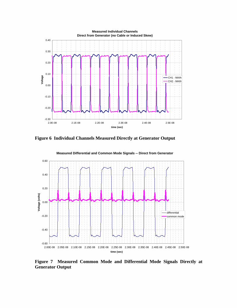
Figure 6 Individual Channels Measured Directly at Generator Output Figure 7 Measured Common Mode and Differential Mode Signals Directly at Generator Output

Measured Individual Channels Direct from Generator (no Cable or Induced Skew)

-0.30

-0.20

-0.10

0.00

0.10

0.20

0.30

0.40

2.0E-08 2.1E-08 2.2E-08 2.3E-08 2.4E-08 2.5E-08

time (sec)

Volta

ge CH1 - MAINCH2 - MAIN

Measured Differential and Common Mode Signals -- Direct from Generator

-0.60

-0.40

-0.20

0.00

0.20

0.40

0.60

2.00E-08 2.05E-08 2.10E-08 2.15E-08 2.20E-08 2.25E-08 2.30E-08 2.35E-08 2.40E-08 2.45E-08 2.50E-08

time (sec)

Volta

ge (v

olts

)

differentialcommon mode

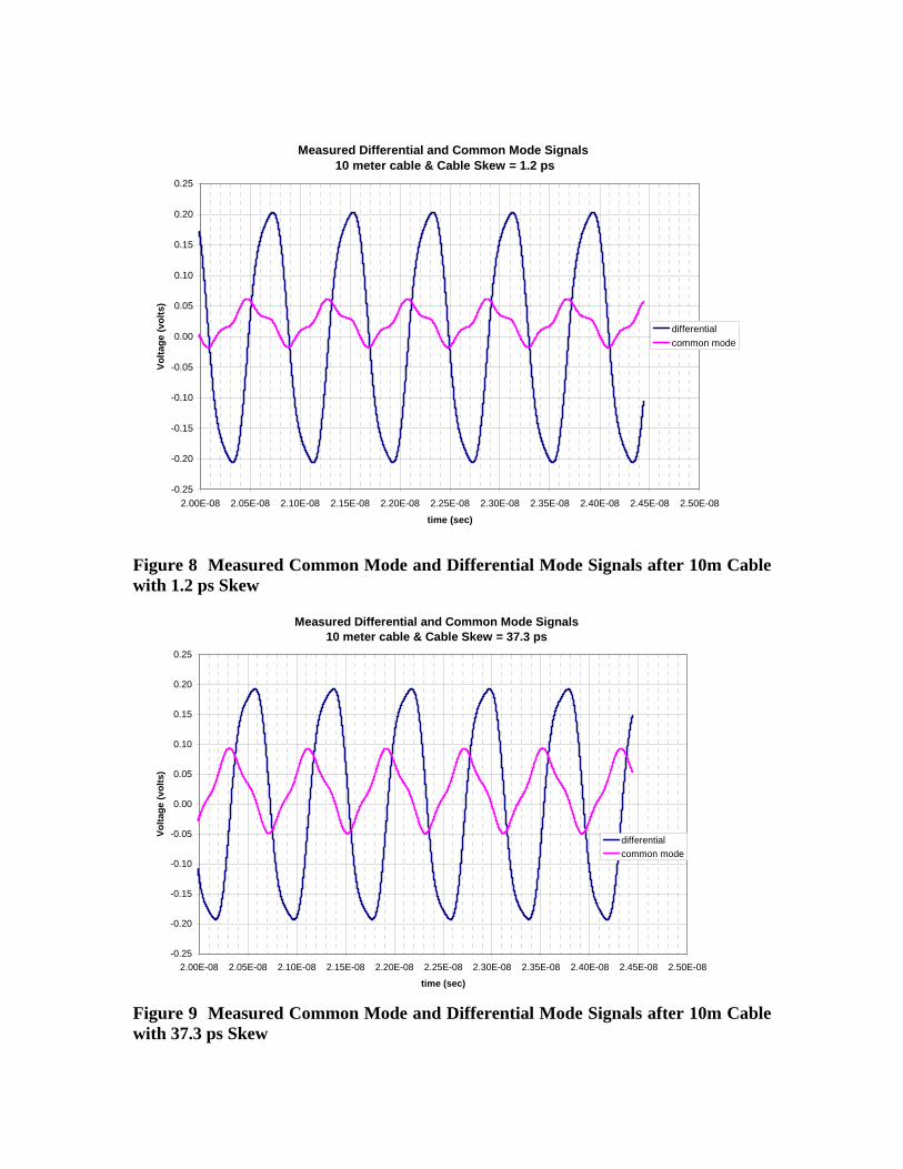
Figure 8 Measured Common Mode and Differential Mode Signals after 10m Cable with 1.2 ps Skew Figure 9 Measured Common Mode and Differential Mode Signals after 10m Cable with 37.3 ps Skew

Measured Differential and Common Mode Signals 10 meter cable & Cable Skew = 1.2 ps

-0.25

-0.20

-0.15

-0.10

-0.05

0.00

0.05

0.10

0.15

0.20

0.25

2.00E-08 2.05E-08 2.10E-08 2.15E-08 2.20E-08 2.25E-08 2.30E-08 2.35E-08 2.40E-08 2.45E-08 2.50E-08

time (sec)

Volta

ge (v

olts

)

differentialcommon mode

Measured Differential and Common Mode Signals 10 meter cable & Cable Skew = 37.3 ps

-0.25

-0.20

-0.15

-0.10

-0.05

0.00

0.05

0.10

0.15

0.20

0.25

2.00E-08 2.05E-08 2.10E-08 2.15E-08 2.20E-08 2.25E-08 2.30E-08 2.35E-08 2.40E-08 2.45E-08 2.50E-08

time (sec)

Volta

ge (v

olts

)

differentialcommon mode

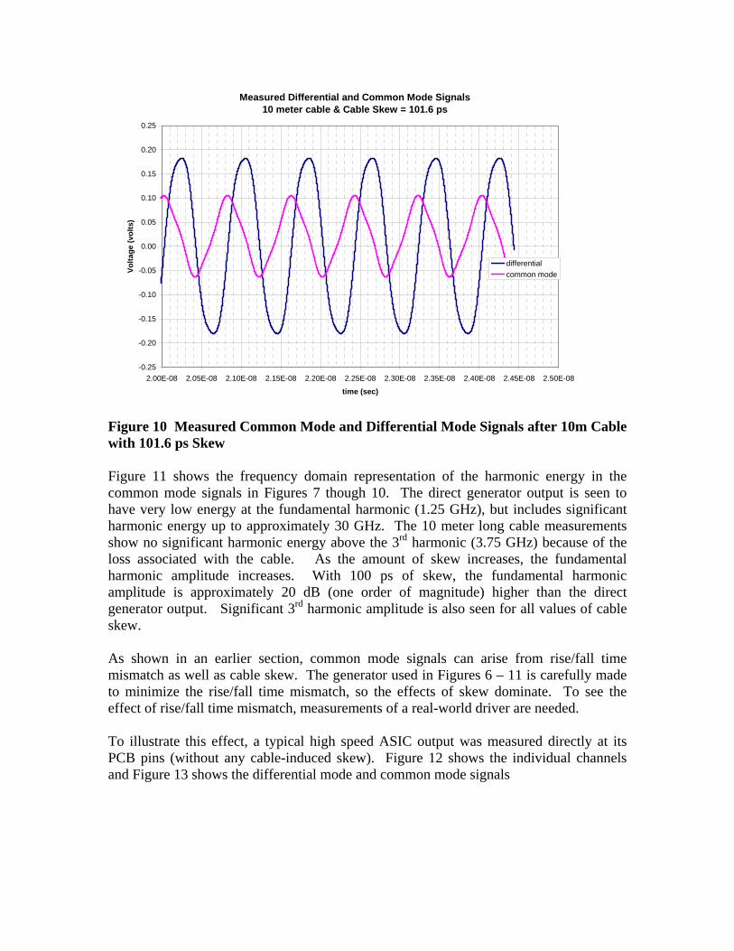
Figure 10 Measured Common Mode and Differential Mode Signals after 10m Cable with 101.6 ps Skew Figure 11 shows the frequency domain representation of the harmonic energy in the common mode signals in Figures 7 though 10. The direct generator output is seen to have very low energy at the fundamental harmonic (1.25 GHz), but includes significant harmonic energy up to approximately 30 GHz. The 10 meter long cable measurements show no significant harmonic energy above the 3rd harmonic (3.75 GHz) because of the loss associated with the cable. As the amount of skew increases, the fundamental harmonic amplitude increases. With 100 ps of skew, the fundamental harmonic amplitude is approximately 20 dB (one order of magnitude) higher than the direct generator output. Significant 3rd harmonic amplitude is also seen for all values of cable skew. As shown in an earlier section, common mode signals can arise from rise/fall time mismatch as well as cable skew. The generator used in Figures 6 – 11 is carefully made to minimize the rise/fall time mismatch, so the effects of skew dominate. To see the effect of rise/fall time mismatch, measurements of a real-world driver are needed. To illustrate this effect, a typical high speed ASIC output was measured directly at its PCB pins (without any cable-induced skew). Figure 12 shows the individual channels and Figure 13 shows the differential mode and common mode signals

Measured Differential and Common Mode Signals 10 meter cable & Cable Skew = 101.6 ps

-0.25

-0.20

-0.15

-0.10

-0.05

0.00

0.05

0.10

0.15

0.20

0.25

2.00E-08 2.05E-08 2.10E-08 2.15E-08 2.20E-08 2.25E-08 2.30E-08 2.35E-08 2.40E-08 2.45E-08 2.50E-08

time (sec)

Volta

ge (v

olts

)

differentialcommon mode

Figure 11 Frequency Domain Harmonics of Common Mode Signals after 10m Cable with Various Amounts of Skew

Figure 12 Individual channels from Typical ASIC at 2.5 Gb/s

Common Mode Voltage from Measured in-pair Cable Skew2.5 Gb/s Data Rate

20

30

40

50

60

70

80

90

100

1.0E+09 1.0E+10 1.0E+11

Frequency (Hz)

Com

mon

Mod

e Vo

ltage

(dB

uv)

Direct from Generatorskew = 1.2 psskew = 37.3 psskew = 101.6 ps

Measured Individual Channels of Typical ASIC Direct OutputNo Cable Induced Skew

-0.40

-0.30

-0.20

-0.10

0.00

0.10

0.20

0.30

2.00E-08 2.05E-08 2.10E-08 2.15E-08 2.20E-08 2.25E-08 2.30E-08 2.35E-08 2.40E-08 2.45E-08

time

Votla

ge

CH1 - MAINCH2 - MAIN

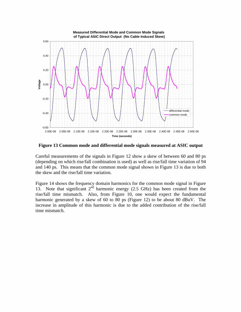
Figure 13 Common mode and differential mode signals measured at ASIC output Careful measurements of the signals in Figure 12 show a skew of between 60 and 80 ps (depending on which rise/fall combination is used) as well as rise/fall time variation of 94 and 140 ps. This means that the common mode signal shown in Figure 13 is due to both the skew and the rise/fall time variation. Figure 14 shows the frequency domain harmonics for the common mode signal in Figure 13. Note that significant 2nd harmonic energy (2.5 GHz) has been created from the rise/fall time mismatch. Also, from Figure 10, one would expect the fundamental harmonic generated by a skew of 60 to 80 ps (Figure 12) to be about 80 dBuV. The increase in amplitude of this harmonic is due to the added contribution of the rise/fall time mismatch.

Measured Differential Mode and Common Mode Signals of Typical ASIC Direct Output (No Cable Induced Skew)

-0.60

-0.40

-0.20

0.00

0.20

0.40

0.60

2.00E-08 2.05E-08 2.10E-08 2.15E-08 2.20E-08 2.25E-08 2.30E-08 2.35E-08 2.40E-08 2.45E-08 2.50E-08

Time (seconds)

Votla

ge

differential modecommon mode

Figure 14 Frequency Domain Harmonics of Common Mode from ASIC with Both Skew and Rise/Fall Time Mismatch Measured Consistency of Skew Introduced in the Cable The previous sections showed how large common mode signals can be created with relatively minor amounts of skew and rise/fall time mismatch. A number of cables were measured to determine the amount of in-pair skew caused by the cables. This is important for EMI/EMC since the EMI/EMC radiated emissions test must be performed with a full system, and this usually means the cables must be connected (and active). InfiniBand Cable Measurements The first set of data comes from 12X (24 pair) InfiniBandTM1 cables. Nine different cables with lengths of eight to ten meters were measured using a differential Time Domain Reflectometer (TDR), with skew measurements by Time Domain Transmission. These cables are intended to be used for 2.5 Gb/s signals with 400 ps pulse width. As shown in Figure 15, the greatest percentage of in-pair skew that was introduced was between 10 – 50 ps of skew (2.5 – 12.5 % of the pulse width). The highest skew measured was 130 ps (32.5% of pulse width), compared to a recommended maximum of 120 ps. Using the data in Figures 1 and 3, the 12% measured skew would result in approximately 450 millivolts (peak) for a one volt normalized signal. Typical InfiniBand

1 InfiniBand is a trademark of the InfiniBand Trade Association

ASIC Driver with Both Skew and Rise/Fall Time Mismatch

20

30

40

50

60

70

80

90

1.0E+09 1.0E+10 1.0E+11

Frequency (Hz)

Com

mon

Mod

e Vo

ltage

(dB

uv)

Direct

signals are 1.2 – 1.6 volts, resulting in an expected scaled common mode voltage of 540 to 720 millivolts. A rule of thumb typically used for radiated EMI emissions is that in order to meet FCC Class B, a product must have less than 100 microvolts of RF noise on an unshielded wire. If this is adjusted for Class A (+10 dB) using the relaxed FCC limit above 1 GHz, then one can use the rule of thumb that the noise level on an unshielded wire should be less than 600 microvolts. The likely common mode voltage from the in-pair cable skew is approximately 60 dB (factor of 1000) higher, meaning that the cable must have about 60 dB minimum of shielding in order to meet EMI radiated emissions limits. This amount of shielding would require careful attention to cable backshell and gasketing. Another consideration is the consistency of skew from cable to cable. Figure 16 shows the skew from all the cables individually. While this is a difficult figure to read, it is obvious that there is no commonality between cables for the amount of skew to expect from the cable. Figure 15 Histogram of In-pair Skew of Nine InfiniBand Cables

IB Cable Skew Percentage Histogram (2.5 Gb/s -- 400 ps Pulse Width)(9 cables with 24 pairs each for 10 m Cables)

0

2

4

6

8

10

12

14

16

18

20

0 10 20 30 40 50 60 70 80 90 100 110 120 130

Amount of Skew (ps)

Per

cent

age

of N

umbe

r of O

ccur

ance

s (%

)

0

20

40

60

80

100

cable 1cable 2

cable 3cable 4

cable 5cable 6

cable 7cable 80

2

4

6

8

no. pairs

skew, ps

In-pair skew by cable sample

cable 1cable 2cable 3cable 4cable 5cable 6cable 7cable 8

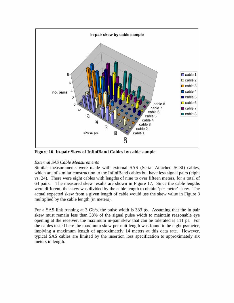
Figure 16 In-pair Skew of InfiniBand Cables by cable sample External SAS Cable Measurements Similar measurements were made with external SAS (Serial Attached SCSI) cables, which are of similar construction to the InfiniBand cables but have less signal pairs (eight vs. 24). There were eight cables with lengths of nine to over fifteen meters, for a total of 64 pairs. The measured skew results are shown in Figure 17. Since the cable lengths were different, the skew was divided by the cable length to obtain ‘per meter’ skew. The actual expected skew from a given length of cable would use the skew value in Figure 8 multiplied by the cable length (in meters). For a SAS link running at 3 Gb/s, the pulse width is 333 ps. Assuming that the in-pair skew must remain less than 33% of the signal pulse width to maintain reasonable eye opening at the receiver, the maximum in-pair skew that can be tolerated is 111 ps. For the cables tested here the maximum skew per unit length was found to be eight ps/meter, implying a maximum length of approximately 14 meters at this data rate. However, typical SAS cables are limited by the insertion loss specification to approximately six meters in length.

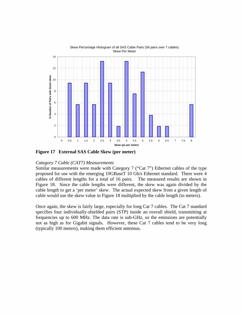
Figure 17 External SAS Cable Skew (per meter) Category 7 Cable (CAT7) Measurements Similar measurements were made with Category 7 (“Cat 7”) Ethernet cables of the type proposed for use with the emerging 10GBaseT 10 Gb/s Ethernet standard. There were 4 cables of different lengths for a total of 16 pairs. The measured results are shown in Figure 18. Since the cable lengths were different, the skew was again divided by the cable length to get a ‘per meter’ skew. The actual expected skew from a given length of cable would use the skew value in Figure 18 multiplied by the cable length (in meters). Once again, the skew is fairly large, especially for long Cat 7 cables. The Cat 7 standard specifies four individually-shielded pairs (STP) inside an overall shield, transmitting at frequencies up to 600 MHz. The data rate is sub-GHz, so the emissions are potentially not as high as for Gigabit signals. However, these Cat 7 cables tend to be very long (typically 100 meters), making them efficient antennas.

Skew Percentage Histogram of all SAS Cable Pairs (56 pairs over 7 cables)Skew Per Meter

0

2

4

6

8

10

12

14

0 0.5 1 1.5 2 2.5 3 3.5 4 4.5 5 5.5 6 6.5 7 7.5 8

Skew (ps per meter)

% N

umbe

r of P

airs

with

Giv

en s

kew

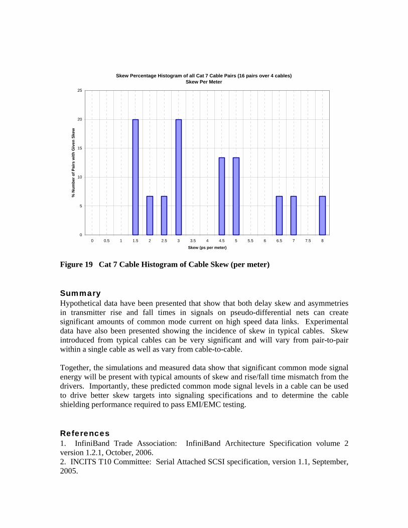
Figure 19 Cat 7 Cable Histogram of Cable Skew (per meter) Summary Hypothetical data have been presented that show that both delay skew and asymmetries in transmitter rise and fall times in signals on pseudo-differential nets can create significant amounts of common mode current on high speed data links. Experimental data have also been presented showing the incidence of skew in typical cables. Skew introduced from typical cables can be very significant and will vary from pair-to-pair within a single cable as well as vary from cable-to-cable. Together, the simulations and measured data show that significant common mode signal energy will be present with typical amounts of skew and rise/fall time mismatch from the drivers. Importantly, these predicted common mode signal levels in a cable can be used to drive better skew targets into signaling specifications and to determine the cable shielding performance required to pass EMI/EMC testing. References 1. InfiniBand Trade Association: InfiniBand Architecture Specification volume 2 version 1.2.1, October, 2006. 2. INCITS T10 Committee: Serial Attached SCSI specification, version 1.1, September, 2005.

Skew Percentage Histogram of all Cat 7 Cable Pairs (16 pairs over 4 cables)Skew Per Meter

0

5

10

15

20

25

0 0.5 1 1.5 2 2.5 3 3.5 4 4.5 5 5.5 6 6.5 7 7.5 8

Skew (ps per meter)

% N

umbe

r of P

airs

with

Giv

en S

kew